A machine learning approach to reconstruction of heart surface potentials from body surface potentials

Abstract

Invasive cardiac catheterisation is a common procedure that is carried out before surgical intervention. Yet, invasive cardiac diagnostics are full of risks, especially for young children. Decades of research has been conducted on the so called inverse problem of electrocardiography, which can be used to reconstruct Heart Surface Potentials (HSPs) from Body Surface Potentials (BSPs), for non-invasive diagnostics. State of the art solutions to the inverse problem are unsatisfactory, since the inverse problem is known to be ill-posed. In this paper we propose a novel approach to reconstructing HSPs from BSPs using a Time-Delay Artificial Neural Network (TDANN). We first design the TDANN architecture, and then develop an iterative search space algorithm to find the parameters of the TDANN, which results in the best overall HSP prediction. We use real-world recorded BSPs and HSPs from individuals suffering from serious cardiac conditions to validate our TDANN. The results are encouraging, in that coefficients obtained by correlating the predicted HSP with the recorded patient’ HSP approach ideal values.

1 Introduction and Related Work

Cardiac catheterisation is an essential procedure carried out to diagnose heart tissue ailments before surgical interventions. Catheterisation is associated with risks such as stroke, heart attacks, and even death [1], especially among young children [2, 3]. Unlike catheterisation, Body Surface Potentials (BSP), captured non-invasively, can potentially be used for diagnosis. The primary idea is to reconstruct the Heart Surface Potentials, (HSP), used for diagnosis, from the BSPs.

The traditional approach to solving this reconstruction problem is to first model the human torso as a series of Partial Differential Equations (PDE), which relates the BSPs and HSPs and then inverting this torso model to produce the HSPs from BSPs. Finding a solution to the inverted torso model is termed the inverse problem of electrocardiography [4]. The inverse problem of electrocardiography is mathematically proven [4, 5] to be ill-posed. Thus, small changes in the BSP inputs can lead to distortions and unbounded errors in the HSP outputs [5].

Given $N$ BSPs, represented by the vector $\Phi_{B}$ and $M$ HSPs, represented by vector $\Phi_{H}$. The inverse problem is given by the linear matrix equation $\Phi_{B}=T_{BH}\times\Phi_{H}$. A number of techniques from standard numerical analysis have been proposed to approximate solutions to the transfer matrix $T_{BH}$. A good overview is provided in [6]. The primary idea in all proposed techniques and their variants is to select elements of the matrix $T_{BH}$ such that the error $\|\Phi_{B}-T_{BH}\times\Phi_{H}\|^{2}$ , is minimized.

The very large search space of the aforementioned minimization problem is reduced by the technique called Tikhonov regularization [7], where the minimization objective is transformed to: $\|\Phi_{B}-T_{BH}\times\Phi_{H}\|^{2}+\gamma\times\|\mathbf{C}\times\Phi_{H}\|^{2}$, where $M\times M$ matrix $\mathbf{C}$ is the discrete approximation of the surface laplacian, and $\gamma$ is the regularization parameter, which controls the weight of the constraint condition. As $\gamma$ approaches zero, the solution oscillates, due to the ill-posed nature of the problem. On the other hand, a large value of $\gamma$ leads to overly smooth solution, unrepresentative of the real HSPs. Hence, the numerical solutions to the regularization problem give unsatisfactory results [8].

Recently, machine learning solutions have been proposed to reconstruct HSPs from BSPs. In [9], kernel ridge regression, with a Gaussian kernel, is used to reconstruct HSPs from BSPs. Although performing better than the numerical solutions, the machine learning solution has low correlation with the exact solution. Hence, the activation map of the heart surface potentials is unsatisfactory. Furthermore, none of the techniques consider reconstruction of HSPs under cardiac disease states, therefore, the fidelity of reconstructed activation map, under diseased states is suspect.

This paper has three major contributions:

1. We propose a neural network model that can predic HSPs from BSPs.

2. We show the efficacy of the proposed neural network model under normal and diseased heart conditions, in particular, for patients suffering from ventricular flutter.

3. We quantify the validity of the HSP activation maps, by correlating them to real-world recorded patient data.

2 A time-delay artificial neural network for predicting heart surface potentials

Our objective is to develop an Artificial Neural Network (ANN) architecture that predicts a single HSP from a single BSP. In this section, we first describe our ANN architecture and then propose search space algorithm to predict parameters of the proposed ANN.

2.1 The basic artificial neural network architecture

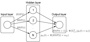
(a) A standard artificial neural network 

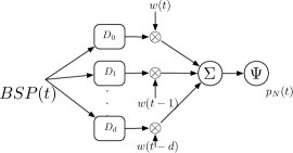
(b) A time-delayed neuron 

Figure 1: The artificial neural network architecture and a time-delayed neuron in the hidden layer

The ANN architecture that forms the basis for predicting the HSP from the BSP is shown in Figure 1a. The ANN consists of three major components: ① an input layer that reads the input signal(s). In our case the input layer consists of a single neuron (shown as a circle), which reads the BSP time series. ② A hidden layer, which consists of $N$ neurons, which learn the relationship between the BSP and the HSP. ③ An output layer, which produces the HSP. In our case the output layer consists of a single neuron, because we produce a single HSP time series. A so called weight (vector), e.g., $w_{N}$ in Figure 1a, and an activation function $\Psi$ are associated with each neuron in the network. The output of a neuron is the inner product of the input vector and the weight vector applied to the activation function.

The number of neurons in the hidden layer, the weight vector associated with each neuron, and the activation function together decide the efficacy of the ANN. Neural network weights are chosen to minimize the mean square error using Levenberg [10] algorithm. Furthermore, the activation function is the sigmoid function. The number of neurons in the hidden layer are chosen using cross-validation techniques described later in Section 2.3.

2.2 Time-delayed artificial neuron

Each neuron uses the current and $d$ previous values of the input BSP to predict the output HSP, at any given point in time, as shown in Figure 1b. Such an ANN architecture is called a Time-Delayed Artificial Neural Network (TDANN) [11]. Hence, for some neuron $N$, in the hidden layer, the output is given by: $p_{N}(t)=\Psi(\Sigma_{j=0}^{d}BSP(t-j)\times w(t-j))$. We use a TDANN, because there is a very high correlation between any point in the BSP(t) and its previous values BSP(t-1), BSP(t-2), $\ldots$, BSP(t-d), since heart has a rhythm under normal and diseased states.

2.3 Training the time-delayed artificial neural network

There are three parameters that need to be tuned in our TDANN: ① the number of neurons $N$ in the hidden layer, ② the weight vector of each neuron in the network, and ③ the time-delay window $d$ for each neuron in the hidden layer. We perform exhaustive search space exploration, using iterative approach to tune the three parameters. The search space exploration algorithm, in Matlab, is given in Figure 2.

Given $P$ patient data, we use $P-1$ BSP and HSP time series for training the TDANN and one patient recording footage for testing purposes. In Figure 2, BSP1, BSP2, HSP1, and HSP2, represent the training input and output datasets, respectively. BSP3 and HSP3 are the test datasets. First the training input and output sets are concatenated together into a single time series vector (lines 2 and 2). Next, the maximum delay window size $d=20$ is initialized. This value is obtained using autocorrelation of BSP training time series. Next, a vector of neurons in the hidden layer is initialized (line 2). In this case, a row vector of 1-20 neurons and then 40, 80, and 100 neurons will be explored during the execution of the iterative algorithm. Line 2 initializes the variable that will hold the best Pearson correlation coefficient for the test dataset during search space exploration.

The actual iteration, selecting the best number of neurons in the hidden layer and the time delay window happens from lines 2-2. The algorithm iterates through each neuron in the neurons vector, and for each hidden layer size, iterates through each possible delay window size. Line 2 initializes the TDANN. Line 2 trains the network over the training dataset. During training, the weight vector for each neuron is obtained using Levenberg minimization algorithm [10]. Next, the algorithm uses the never seen before test dataset BSP3 to predict the heart surface potential output (PHSP3) and correlates it to the actual HSP3 dataset. The net, along with its configuration, that gives the best correlation coefficient is stored for later use (lines 2-line 2).

clear; clc; %% Training on patient-1 and patient-2 together train_input = dtrend([BSP1(s:e); BSP2(s:e)]); train_output = dtrend([HSP1(s:e); HSP2(s:e)]); d = 20; %% The maximum delay %% The neuron vector neurons = [1:1:20, 40, 80, 100]; maxC = 0.0 for n = 1:size(neurons)(2)   % Iterate through neurons  for delay = 1:d % Iterate through delay   [X, ~] = tonndata(train_input, false, false);   [T, ~] = tonndata(train_output, false, false);   %% Initialize a time-delay network   net = timedelaynet((0:delay), neurons(n),                      ’trainlm’);   %% Train the network.   %% Selecting weights via levenberg algorithm   [Xs,Xi,Ai,Ts] = preparets(net,X,T);   net = train(net,Xs,Ts, Xi, Ai);   % compute correlation coefficient   % for never seen before test-patient.   % PHSP3 is the predicted output for BSP3   PHSP3 = net(BSP3(s:e), false, false,              BSP3(s:s+(delay-1)), false, false);   C = corr(HSP3, PHSP3(s:e)); % pearson correlation   if C > maxC    maxC = C;    %% Store result    result = [net, maxC, neurons(n), delay];   end  end end

Figure 2: The algorithm to tune TDANN parameters

3 Experimental Benchmarking

In this section we describe the efficacy of the proposed TDANN using real-world patient recordings.

3.1 Experimental setup

We use the BSP and HSP data recorded from patients, available in [12]. We use the BSP recorded from Lead I of the electrocardiogram machine as the input and the unipolar HSP recorded, at the same time, from the Right-Ventricular Apex, as the output, for all our experiments. The TDANN training and testing algorithm is designed in Matlab version R2016b, running on OSX 10.11.6, Intel Core i5 2.9 GHz laptop with 8 GB of RAM.

Patient ID	Heart rhythm	Start (sec)	End (sec)	Used for
343220	Normal rhythm	1	10000	Training
33093	Normal rhythm	1	10000	Training
343220	Normal rhythm	3000	65000	Validation
33093	Normal rhythm	3000	65000	Validation
221708	Normal rhythm	1	65000	Testing
343300	Ventricular flutter	3000	6000	Training & Validation
176230	Ventricular flutter	3000	6000	Training & Validation
198a385	Ventricular flutter	10000	15000	Testing

Table 1: Patient data used for experiments

The patient data from [12] used in our experiments is tabulated in Table 1. Column-1 lists the specific footage used for experiments from the database. Column-2 lists the heart condition. We trained our TDANN to predict HSP under normal heart rate and ventricular flutter. Ventricular flutter is especially important, because it is transient and can lead to death. Next the table lists the starting and ending seconds of the complete footage that was used for experiments. Finally, the table lists the reason for using each of these footages, some were used for training, while others were used for cross-validation and testing purposes.

3.2 Results

We present two sets of results: ① the pearson correlation coefficients obtained from the best trained neural nets for the validation and testing datasets from Table 1. We use the training algorithm described previously in Figure 2. ② The affect on prediction accuracy with changing delay window ($d$) and number of neurons ($N$) in the hidden layer. In all the figures that follow, we plot only a part of the correlated time-series for ease of understanding.

Figure 3: Validation result Patient: 33093, normal heart rhythm, correlation coefficient: 0.7, $N=11$, $d=15$.

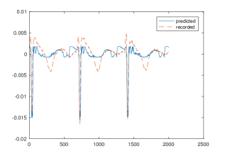
Figure 4: Validation result Patient: 343330, normal heart rhythm, correlation coefficient: 0.7519, $N=11$, $d=15$.

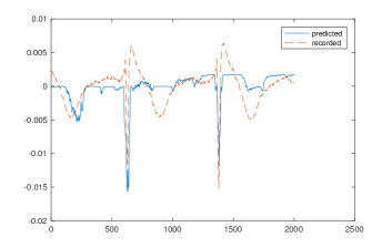
Figure 5: Test result Patient: 221708, normal heart rhythm, correlation coefficient: 0.5122, $N=11$, $d=15$.

Figures 3-5 correlate the predicted HSP with the recorded patient HSP at the right ventricular atrium under normal heart rhythm. In all cases the results are quite consistent. Especially note that the voltage peaks are consistently met in all cases, a problem that is faced by the current state of the art techniques.

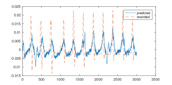
Figure 6: Validation result Patient: 343330, ventricular flutter, correlation coefficient: 0.45536, $N=5$, $d=18$.

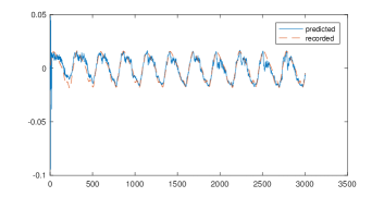
Figure 7: Validation result Patient: 176230, ventricular flutter, correlation coefficient: 0.9, $N=5$, $d=18$.

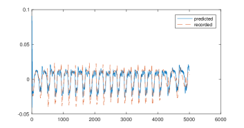
Figure 8: Test result Patient: 198a385, ventricular flutter, correlation coefficient: 0.8171, $N=5$, $d=18$.

Figures 6-8 correlate the predicted output and the patient recorded HSP output, at the right ventricular apex, under ventricular flutter. In this case, the correlation coefficient approach 0.9, with an average for the three patients at 0.7. These values are very close to the ideal value of 1.0. Hence, this shows that our TDANN approach is a good option for predicting HSP from BSP.

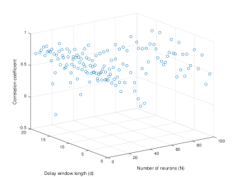
Figure 9: Affect of changing delay window size ($d$) and number of neurons ($N$) for the test dataset 198a385

It is worth noting that, in both cases, very few neurons and a small delay window is needed. In fact, increasing the number of neurons and the delay window ($d$) leads to over-fitting the output to the training dataset (see Figure 9, for example). Our iterative algorithm (Figure 2) overcomes these over-fitting problems, by exploring the complete search space of possible solutions.

4 Conclusions and future work

In this paper we describe an artificial neural network approach to predicting heart surface potentials from body surface potentials. Predicting heart surface potentials non-invasively, can potentially be used in the future for non-invasive cardiac diagnostics. Our primary idea is to build time-delay neural networks for predicting single heart surface potential from a single body surface potential. Time-delay neural network, allows for using past values of the input body surface potential to predict the heart surface potential. We develop an iterative search space exploration technique to find the number of neurons needed in the hidden layer along with the delay window size. The prediction results are very encouraging, in that the Pearson coefficients correlating predicted and recorded heart surface potentials approach the ideal value under normal and diseased heart states. We have shown the efficacy of our approach using real-world recorded patient data.

In the future we plan to enhance the presented approach with multiple body surface potential recordings to predict the heart surface potentials.

References

- [1] M. Al-Hijji, R. Lennon, R. Gulati, J. Y. Park, D. Crusan, A. Kanwar, A. Behfar, A. Lerman, G. S. Sandhu, D. Holmes, et al., “Safety and risk of diagnostic cardiac catheterization,” 2017.
- [2] J. Kreutzer, “Catastrophic adverse events during cardiac catheterization in pediatric pulmonary hypertension may not be so rare,” 2015.
- [3] M. L. O’Byrne, A. C. Glatz, B. D. Hanna, R. T. Shinohara, M. J. Gillespie, Y. Dori, J. J. Rome, and S. M. Kawut, “Predictors of catastrophic adverse outcomes in children with pulmonary hypertension undergoing cardiac catheterization: a multi-institutional analysis from the pediatric health information systems database,” Journal of the American College of Cardiology, vol. 66, no. 11, pp. 1261–1269, 2015.
- [4] Y. Rudy and B. Messinger-Rapport, “The inverse problem in electrocardiography: solutions in terms of epicardial potentials.” Critical reviews in biomedical engineering, vol. 16, no. 3, pp. 215–268, 1988.
- [5] M. Hullerum, “The inverse Problem of Electrocardiography,” 2012.
- [6] R. M. Gulrajani, “The forward and inverse problems of electrocardiography,” IEEE Engineering in Medicine and Biology Magazine, vol. 17, no. 5, pp. 84–101, 1998.
- [7] A. N. Tikhonov, V. I. Arsenin, and F. John, Solutions of ill-posed problems. Winston Washington, DC, 1977, vol. 14.
- [8] S. Ghosh and Y. Rudy, “Application of l1-norm regularization to epicardial potential solution of the inverse electrocardiography problem,” Annals of biomedical engineering, vol. 37, no. 5, pp. 902–912, 2009.
- [9] N. Zemzemi, R. Dubois, Y. Coudiere, O. Bernus, and M. Haissaguerre, “A machine learning regularization of the inverse problem in electrocardiography imaging,” in Computing in Cardiology Conference (CinC), 2013. IEEE, 2013, pp. 1135–1138.
- [10] J. J. Moré, “The levenberg-marquardt algorithm: implementation and theory,” in Numerical analysis. Springer, 1978, pp. 105–116.
- [11] A. Waibel, T. Hanazawa, G. Hinton, K. Shikano, and K. J. Lang, “Phoneme recognition using time-delay neural networks,” IEEE transactions on acoustics, speech, and signal processing, vol. 37, no. 3, pp. 328–339, 1989.
- [12] Ann Arbor Electrogram Libraries, “Chicago, Illinois, USA,” http://electrogram.com/.