Weighted Delta-Tracking in Scattering Media

Abstract

In this work, we expand the weighted delta-tracking routine to include a treatment for scattering. The weighted delta-tracking routine adds survival biasing to normal delta-tracking, improving problem figure of merit. In the original formulation of this method, only absorption events were considered. We have expanded the method to include scattering and investigated the method’s effectiveness with two test cases: a pressurized water reactor pin cell and a fast reactor pin cell. We compare the figure of merit for calculating infinite flux and total cross-section while incrementally changing the amount of weighted delta-tracking used. We find that this new weighted delta-tracking (WDT) routine has strong potential to improve the efficiency of fast reactor calculations, and may be useful for light water reactor calculations.

1 Introduction

Monte Carlo methods have been used to model neutron transport since first introduced at Los Alamos National Lab by Metropolis and Ulam [9]. Over the last 60 years, the method has been adapted to new computer architectures and expanded to improve the efficiency and accuracy of calculations. At the core of Monte Carlo simulations is the statistics of simulating repeated events, so improving the accuracy of results either requires more events or a more efficient use of events. In transport calculations, particle collision events are commonly and effectively used to calculate reaction rates and fluxes.

Modern Monte Carlo codes use many techniques to improve efficiency and in many cases operate alongside deterministic codes. These improvements and hybrid methods have advanced the scale and types of problems that users can simulate. The field is now seeking to solve full-core simulations, coupled multiphysics models, and other problems on the edge of our computational capability. One such use of multiphysics models that seeks to support development of advanced reactor fuels is for the restart of the Transient Reactor Test Facility (TREAT) at the Idaho National Lab (INL) [10]. There, researchers are using the Serpent 2 Monte Carlo code [2] to generate multigroup cross-sections for the Rattlesnake deterministic code.

To advance these complex models, more efficient methods that require less clock time are needed. One such improvement was the introduction of Woodcock delta-tracking [12]. Delta-tracking mitigates some inefficiencies that occur when standard ray tracing is used for geometries with optically thin regions, but introduces new well-documented difficulties in the presence of heavy absorbing materials [3][8]. A new method, WDT, was introduced by Morgan and Kotlyar [8] to modify the delta-tracking routine to use weight reduction in place of rejection sampling.

In this paper, we will begin by providing background discussion about the neutron propagation techniques ray tracing, delta-tracking, and the WDT routine of Morgan and Kotlyar. We will then describe the new work: a novel modification of the WDT routine that extends the method to include scattering. This extension is a hybrid of WDT and normal delta-tracking that seeks to be more efficient than either independently. Including scattering enables us to evaluate the WDT method in two common test problems: a pressurized water reactor (PWR) pin cell and a fast reactor pin cell. We will then examine the results of these simulations and compare them to a base case where the new routine is not used. Finally, we will discuss those results and make a recommendation for the use of WDT in these types of problems.

2 Background

At the core of every Monte Carlo neutron transport simulation is the propagation of the particles through material regions. Ray tracing is a straightforward method for sampling the path length, how far a neutron will travel before interacting with the local material. The algorithm samples the path length $s$ of a propagating neutron at a position $\bm{r}$ and with energy $E$ using

$$s(\xi,\bm{r},E)=-\frac{1}{\Sigma_{t}(\bm{r},E)}\ln(\xi)\>,$$ (1)

where $\xi$ is a uniformly distributed random variable $\xi\in[0,1)$, and $\Sigma_{t}(\bm{r},E)$ is the total macroscopic cross-section.

The macroscopic cross-section depends on the current material, and is therefore a discontinuous function that varies with position and the material geometry of the problem [4]. A path length sampled using Eq. (1) becomes statistically invalid if the neutron crosses into a material region with a different macroscopic cross-section. Therefore, each time a new path length is sampled, we must calculate the distance to the nearest boundary along the propagation path. Then, if the neutron will cross into a new material region, the distance to interaction past the boundary must be recalculated.

These two processes cause boundaries to contribute to the computational work of the ray tracing routine. This overhead can cause significant inefficiencies in complex geometries or optically thin regions. Various methods have been developed to overcome these regions of high cost, one of which is Woodcock Delta Tracking.

2.1 Woodcock delta-tracking

Woodcock introduced the delta-tracking method for neutron propagation in 1965 [12]; in modern Monte Carlo codes it is often offered as an alternative or compliment to the standard ray tracing procedure. The method was designed to address some of the limitations of ray tracing but introduces its own new limitations. Lux and Koblinger [7] provide an overview of the method, and its performance in various codes has been examined by Leppänen [4] and others. A short description of the delta-tracking method is given here to motivate development of the WDT routine.

The Woodcock delta-tracking method chooses a single macroscopic cross-section to calculate path lengths for the entire region of interest, which can include multiple materials. This is chosen to be the maximum of all material total cross-sections, the majorant cross section:

$$\Sigma_{\mathrm{maj}}\equiv\max_{\bm{r}\in\bm{\mathrm{D}}}\{\Sigma_{t}(\bm{r})\}\>,$$ (2)

where $\bm{\mathrm{D}}$ is the region of interest. We relate this value to the actual macroscopic cross-section by introducing an arbitrary $\delta$ cross-section that varies with position,

$$\Sigma_{\mathrm{maj}}=\Sigma_{\delta}(\bm{r})+\Sigma_{t}(\bm{r}),\quad\forall\bm{r}\in\bm{\mathrm{D}}\>.$$ (3)

To maintain the physics of the problem, a delta collision must preserve the energy and direction and existence of the neutron; it must be a “virtual” collision. As a result, these can occur any number of times along a neutron’s path without consequence.

As the majorant cross-section is not a function of position, path lengths sampled using Eq. (1) are valid throughout the region of interest. To replicate sampling the real distribution that is a function of position, we use a rejection-sampling algorithm, thoroughly described by Lux and Koblinger [7]. Following each sampled path length, the collision is real (non-virtual) with a probability related to the cross section at the point of collision,

$$P_{\text{real}}(\bm{r}) =\frac{\Sigma_{t}(\bm{r})}{\Sigma_{\mathrm{maj}}}\>.$$ (4)

Otherwise, the collision is a product of the $\delta$ cross-section and is therefore virtual. In the material with the maximum cross-section, $\Sigma_{t}(\bm{r})=\Sigma_{\text{maj}}$, all collisions are real. The algorithm for delta-tracking is shown in Alg. 1.

Algorithm 1 Delta-tracking

1:Sample path length, $s$

2:Propagate neutron

3:Look up material at neutron position to get $\Sigma_{t}(\bm{r})$

4:$P_{\mathrm{real}}\leftarrow\frac{\Sigma_{t}(\bm{r})}{\Sigma_{\mathrm{maj}}}$

5:Sample random number $\xi\in[0,1)$

6:if $\xi<P_{\mathrm{real}}$ then

7:     Execute real collision

8:else

9:     Execute virtual collision

10:end if

The delta tracking routine provides the ability to sample a path length that is valid throughout the entire region of interest, unlike ray tracing. Some of the inefficiency of ray tracing in optically thin or complex geometries is mitigated. However, lookup is still required for the cross section at the point of collision, and an extra random number must be sampled.

This routine introduces its own inefficiencies. These can occur in regions where $\Sigma_{t}(\bm{r})\ll\Sigma_{\text{maj}}$ and the probability of a real collision is low, as in streaming regions near strong absorbers. In these regions, many virtual collisions occur, and the computational expense out-weighs the little statistical information provided. We will describe two approaches to counteract this: the first is a combination of ray tracing and delta-tracking, and the second is a method called weighted delta-tracking.

2.2 Delta-tracking with ray tracing

Since delta-tracking can be computationally inefficient in regions where the probability of a real collision is low, we can attempt to mitigate this by switching back to a ray tracing routine in those regions. An example of this approach is presented here, as it is implemented in the Serpent 2 Monte Carlo code.

Serpent was developed at VTT Technical Research Centre of Finland (VTT) by Jaakko Leppänen [2], and a second iteration of the code, Serpent 2, is under active development. Both versions of Serpent use a combination of ray-tracing and Woodcock delta-tracking for sampling path length. Serpent selects between ray tracing and delta-tracking by examining the ratio of total cross-section to majorant cross-section [3], giving the value of $P_{\mathrm{real}}$. In regions where many virtual collisions would occur, the code preferentially switches to ray tracing. This is to avoid the computational inefficiency identified in the previous section. This selection is determined by a constant $c$ and the following inequality, which is identical to our formulation of $P_{\mathrm{real}}$:

$$\frac{\Sigma_{t}(\bm{r})}{\Sigma_{\mathrm{maj}}}=P_{\text{real}}>1-c\>.$$ (5)

If this inequality is satisfied, delta-tracking is used, otherwise ray tracing is used. By default, the value of $c$ is 0.9, empirically determined to produce the largest improvement in run time [3]. Prior to sampling path length, the code tests this ratio for the current neutron position and determines which path length sampling algorithm should be used.

2.3 Weighted delta-tracking

Morgan and Kotlyar [8] introduced a different approach to improve the inefficiencies of Woodcock delta-tracking in the presence of large absorbers. The method, WDT, replaces the rejection sampling of delta-tracking with a statistical weight reduction.

Statistical weight is an often-used mathematical concept that describes the percentage of a neutron still available to contribute to a response. For example, the collision estimator gives an estimate for scalar flux $\phi$ based on the neutron’s weight prior to collision $w_{i}$ and the total cross-section, summed over all collisions $C$,

$$\phi=\frac{1}{W}\sum_{C}\frac{w_{i}}{\Sigma_{t}(\bm{r},E)}\>,$$

where $W$ is the weight of neutrons at generation, which is often unity. A neutron with zero weight is removed from the simulation, because it can no longer contribute to responses.

Neutron weight can be augmented throughout its lifetime through interactions, games played at boundary crossings, etc., so long as a fair game is maintained. Weight change methods such as survival biasing improve the efficiency of simulations by keeping particles alive longer, allowing them to contribute more information to the solution with the goal of improving statistics. Details of different methods for variance reduction are outside the scope of this work. The main points are that weight corresponds to contribution to the solution of interest, weight can be changed based on a particle’s history, and a fair game must be maintained.

The WDT method samples the particle path length in the same fashion as Woodcock delta-tracking, using the majorant cross-section. Unlike the delta-tracking routine, WDT accepts all collisions as real. To keep a fair game, the neutron’s weight must be changed to account for the virtual collisions that no longer occur explicitly. Each collision can result in multiple outcomes, each of which is mutually exclusive. To calculate the change in weight, we use the expected value of the interaction. The outcomes are real and virtual collisions, which result in final weights $w_{f,\mathrm{virt}}$ and $w_{f,\mathrm{real}}$, respectively. The final neutron weight is therefore given by

$$E[w_{f}]=w_{f,\mathrm{real}}P_{\mathrm{real}}+w_{f,\mathrm{virt}}\left(1-P_{\mathrm{real}}\right)\>.$$ (6)

An absorption event removes the particle from the simulation, so the resulting final weight of a real collision is zero. A virtual collision is a scattering event, and therefore leaves the weight unchanged. Inserting the appropriate values into Eq. (6) gives the expected value of the final weight for an absorption event for a neutron with initial weight $w_{i}$:

$$E[w_{f},\bm{r}] =w_{f,\mathrm{real}}P_{\mathrm{real}}(\bm{r})+w_{f,\mathrm{virt}}(1-P_{\mathrm{real}}(\bm{r}))$$

$$=w_{i}\left(1-P_{\mathrm{real}}(\bm{r})\right)\>.$$

The particle then continues propagating as if it underwent a virtual collision. The removed statistical weight is then added to the appropriate responses, such as collision tallies.

The key change in WDT is that unlike normal delta-tracking, every sampled path length results in a real collision and subsequent contribution to tallies. As discussed earlier, a major inefficiency in delta-tracking is wasted computational resources in regions with many virtual collisions that do not contribute to statistical quality. The WDT method therefore partially mitigates this issue by collecting contributions to tallies with every collision.

This algorithm was implemented by Kotlyar and Morgan and tested using a 1D problem in an absorbing medium. They found an improvement in the computational efficiency of the simulation.

Legrady, Molnar, Klausz, and Major [6] performed an analysis of delta-tracking methods, including WDT. The aim of their study was to quantify the effects of modifying the single cross-section used by the Woodcock delta-tracking method for sampling path lengths. This sampling cross-section is chosen to be the majorant in standard Woodcock delta-tracking and WDT. They find that the optimal sampling cross-section occurs below the majorant in all cases and outperformed the WDT method by a factor of 70 in their test cases. For this study, we will not consider their optimization, and will leave the sampling cross-sections of the standard delta-tracking and WDT processes unmodified.

3 Method

The WDT routine introduced a method to improve the inefficiencies of Woodcock delta-tracking in the presence of large absorbers. The method resulted in an improvement in simulation efficiency in a purely absorbing medium, but did not address how the routine would work with scattering. Therefore, we will need to extend or modify the WDT method to include scattering such that it is applicable to more realistic problems.

We will first attempt to extend WDT in a naïve fashion, by applying the same process for absorption to scattering. We will show that this will result in a process that can become intractable. This will motivate development of a hybrid method that uses both standard delta-tracking and WDT to accommodate scattering events.

3.1 Naïve Extension of Weighted delta-tracking

As previously discussed, in a scattering event the statistical weight of the incident particle does not change. This holds true for a real scattering event as well as a virtual event; from the perspective of neutron weight, the two events are identical. Therefore, application of the WDT weight reduction will result in no overall weight reduction:

$$E[w_{f}] =w_{f,\mathrm{real}}P_{\mathrm{real}}+w_{f,\mathrm{virt}}(1-P_{\mathrm{real}})$$

$$=w_{i}(P_{\mathrm{real}}+1-P_{\mathrm{real}})$$

$$=w_{i}\>.$$

Although the overall statistical weight remains unchanged, portions of it must be added to the appropriate response. The WDT weight reduction splits the statistical weight into two portions: the real portion “experiences” the scattering event, and the virtual portion undergoes a virtual collision. The virtual portion of the weight is retained by the original neutron, which continues with the same direction and energy. We then create a new neutron to receive the real portion and execute a real scattering event.

Therefore, straightforward extension of this methodology to scattering requires doubling of the neutron at every scattering event. In problems with any scattering, this will likely result in a rapid and intractable multiplication of neutrons that will overload memory buffers. In an experimental implementation of this method, that is exactly what we found. Thus, we concluded the naïve extension was not a useful way to include scattering in WDT.

3.2 Hybrid Extension of Weighted delta-tracking

To address the issue of intractable neutron multiplication that comes with the naïve extension of WDT, we created a hybrid version that includes a fallback to the standard delta-tracking method for any scattering events. Following each sampled path length, the type of collision (that will occur if real) must be sampled; we use WDT if the collision is an absorption event, and delta-tracking otherwise. The algorithm is shown in Alg. 2 and a flow chart of the routine is shown in Fig. 1.

Algorithm 2 Weighted delta-tracking with scattering

1:Sample path length

2:Sample collision type

3:if collision type == (capture or fission) then

4:     Score capture or fission $\leftarrow w_{i}P_{\mathrm{real}}$

5:     Score collision $\leftarrow w_{i}P_{\mathrm{real}}$

6:     $w_{f}\leftarrow w_{i}(1-P_{\mathrm{real}})$

7:     Execute virtual collision

8:else

9:     Sample random number $\xi\in[0,1)$

10:     if $\xi<P_{\mathrm{real}}$ then $\triangleright$ Collision is real

11:         Score scattering $\leftarrow w_{i}$

12:         Score collision $\leftarrow w_{i}$

13:         Execute scattering collision

14:     else$\triangleright$ Collision is virtual

15:         Execute virtual collision

16:     end if

17:end if

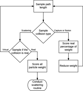
Figure 1: Weighted delta-tracking with scattering rejection sampling.

In highly scattering regions, the routine is expected to be slightly less efficient than standard delta-tracking because every collision requires an extra random number sample and comparison. By contrast, in highly absorbing regions, we aim to benefit from the improved efficiency of the WDT routine compared to delta-tracking.

The efficiency will also depend on the value of $P_{\text{real}}$. At high values of $P_{\mathrm{real}}$, a majority of the weight of the incoming particle is scored. This leaves the particle that undergoes a virtual collision with a very low weight, relying on a rouletting routine [7] to prevent computational inefficiency. In regions of low $P_{\text{real}}$, each collision will only contribute a small amount to the appropriate tallies. We expect this to be more efficient than standard delta-tracking, which generates many virtual collisions in the same region that do not contribute to tallies of interest.

This implies that there is a region between low and high values of $P_{\mathrm{real}}$ where WDT may provide benefit.

We have previously discussed that switching to a ray tracing routine in regions of low $P_{\mathrm{real}}$ is effective in countering the inefficiency of delta-tracking. We therefore combine ray tracing, WDT, and standard delta-tracking together in a scheme defined by two parameters. On the lower end, the value of $P_{\mathrm{ray}}$ defines the value of $P_{\mathrm{real}}$ below which ray tracing is used. On the upper end, $P_{\mathrm{wdt}}$ defines the cutoff below which WDT will be used instead of normal delta-tracking. This scheme is summarized as,

$$\text{Propagation mode }(\bm{r},E)=$$

$$\left\{\begin{array}[]{lrrcl}\text{Ray tracing},&\text{if}&&P_{\mathrm{real}}(\bm{r},E)&<P_{\mathrm{ray}}\\ \text{\lx@glossaries@gls@link{acronym}{wdt}{\leavevmode WDT}},&\text{if}&P_{\mathrm{ray}}\leq&P_{\mathrm{real}}(\bm{r},E)&<P_{\mathrm{wdt}}\\ \text{Delta-tracking},&\text{if}&P_{\mathrm{wdt}}\leq&P_{\mathrm{real}}(\bm{r},E)&\end{array}\right.\>,$$

where $P_{\mathrm{real}}\in[0,1)$ and is shown graphically in Fig. 2.

Figure 2: Implemented selection scheme for propagation mode: ray-tracing, weighted, and normal delta-tracking. Shown using the values of $P_{\mathrm{ray}}=0.1$ and $P_{\mathrm{wdt}}=0.4$.

Implementation in Serpent was straightforward; $P_{\mathrm{ray}}$ is already implemented in the user parameter $c$, where $P_{\mathrm{ray}}=(1-c)$. As discussed in Sec. 2.2, a value of $c=0.9$ or $P_{\mathrm{ray}}=0.1$ resulted in the highest computational efficiency. Examination of the WDT cutoff value, $P_{\mathrm{wdt}}$, is the aim of the remainder of this study. We implemented our hybrid WDT in Serpent 2, with the ability to adjust the value of $P_{\mathrm{wdt}}$. The amount of ray tracing never changes; we are instead adjusting the amount of delta-tracking that is replaced by the WDT routine. By adjusting the value of $P_{\mathrm{wdt}}$ from $P_{\mathrm{ray}}$ (no WDT) to 1.0 (full WDT), we investigate the impact of the routine on computational efficiency.

4 Results & Discussion

We expect that the WDT method will improve the statistics of Serpent calculations. With normal delta-tracking, virtual collisions provide no statistical benefit, and are therefore an inefficient use of computational resources. In contrast, all collisions that result in absorption events contribute to statistics when using WDT. Therefore, we expect an improvement in the results of a Serpent 2 simulation in regions with absorption. We chose two test cases: a fast reactor pin cell and a PWR pin cell. In this section, we will describe those two cases, how we determined quality in the simulation, and the test case results.

4.1 Test Cases

Two test cases were selected to test the performance of the WDT method. These are a PWR pin cell and a fast reactor pin cell. We chose these two test cases to evaluate the method in a domain where absorption is dominant in the fast group (fast pin cell) and one in which absorption is dominant in the thermal group (PWR pin cell). All test cases were run on a small cluster at the University of California, Berkeley, and the specifications of the cluster are shown in Tab. 1.

Table 1: Small cluster specifications

Parameter	Specification
Processor	2 $\times$ TenCore Intel Xeon Processor E5–2687W v3 3.10 GHz 25MB Cache
RAM	16 $\times$ 16GB PC4–17000 2133MHz DDR4
Hard drive	2 $\times$ 800 GB Intel SATA 6.0 GB/s Solid State Drive

4.1.1 Pressurized water reactor pin cell

The PWR pin cell was chosen from the Serpent 2 validation input files provided on the VTT Serpent webpage [11]. The geometry and physical parameters are shown in Fig. 3. The fuel is a 2.68 w/o enriched UO₂ mixture, with Zircaloy cladding, light water moderation, and reflective boundary conditions. The simulation output statistics binned neutrons into two energy groups with the group boundary at 0.625 eV.

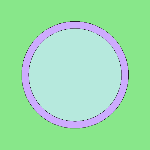
Parameter Value (cm) Fuel radius 0.412 Cladding radius 0.475 Pitch 1.33

Figure 3: Pressurized water reactor geometry and physical parameters. The fuel is shown in light blue, the cladding in purple and the coolant is green.

4.1.2 Fast reactor pin cell

We adapted the fast reactor pin cell from an example provided in the Serpent validation files [11]. This is a lead cooled pin cell with Mixed Oxide (MOX) fuel containing uranium, plutonium, and a small amount of americium. The relative isotope amounts are shown in Tab. 2. The cladding is stainless steel, the lattice is hexagonal, and we used reflective boundary conditions. As with the PWR pin cell, we ran the simulation with two energy groups with the group boundary at 0.625 eV.

Parameter Value (cm) Void radius 0.1 Pellet radius 0.45 Inner cladding radius 0.465 Outer cladding radius 0.525 Pitch 1.789

Figure 4: Fast pin cell geometry and physical parameters. The pellet is shown in blue, the cladding green, and the coolant orange. Black regions are voids.

Table 2: Atomic density of the fast reactor pin cell MOX fuel, values are relative to the atomic density of ²³⁸U

Isotope	Relative Atomic Density
238U	1.00
239Pu	0.16
240Pu	7.40 $\times 10^{-2}$
242Pu	2.09 $\times 10^{-2}$
238Pu	6.45 $\times 10^{-3}$
235U	4.11 $\times 10^{-3}$
241Am	3.57 $\times 10^{-3}$
236U	1.00 $\times 10^{-4}$
234U	3.01 $\times 10^{-5}$

4.2 Cycles per CPU time

All calculations done in this study were criticality source calculations. For these types of calculations in Serpent, source neutrons are run in cycles. Each cycle contains the same number of source neutrons, and the source distribution is determined by the previous cycle [5]. More efficient simulations will be capable of running more cycles, $C$, in a given CPU time frame, $t$. So, to measure one standard of efficiency, we looked at the cycles per CPU time, $C/t$, for each of the two test cases.

Another way to consider method effectiveness is using the average number of real collisions per track. Unlike virtual collisions, real collisions contribute to the statistics of the problem and therefore require tallying and other processes. This makes real collisions more computationally costly than virtual collisions. Based on the WDT and standard delta tracking algorithms, we expect to see an increase in the number of overall real collisions with a subsequent decrease in cycles per CPU time. This apparent reduction in efficiency will be offset by the improved statistics provided by the real collisions. We therefore expect cycles per CPU time and average real collisions per track to have inverted behaviors.

4.2.1 Fast Reactor Pin Cell

The fast reactor pin cell is dominated by absorption; fast neutrons drive fission and little scattering occurs. Our WDT with scattering routine always considers absorption reactions to be real collisions, so we see a rise of the average real collisions per neutron track compared to the standard delta-tracking routine. This is shown in Fig 5(b). At higher levels of the threshold value the number of real collisions levels off, indicating that the WDT routine may be handling a majority of the phase space where absorption occurs. We observe a step increase in average real collisions per track when $P_{\mathrm{wdt}}$ is unity; this is the only value where the WDT routine will be used in the region that defines $\Sigma_{\mathrm{maj}}$. For this test problem the region of highest cross-section is also a highly absorbing region, so use of the WDT routine in that region causes the number of real collisions to increase significantly. We see the inverse pattern in the cycles per CPU time, as anticipated and described in the previous section. The data are shown in the second column of Table 7.

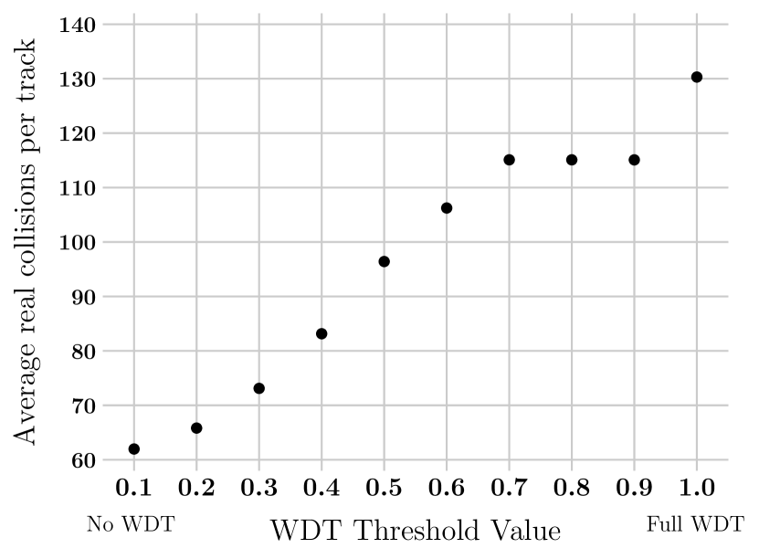
(a)

(b)

Figure 5: For the fast reactor pin cell, (a) cycles per CPU time (normalized to the base case with no WDT) and (b) average real collisions per track, with increasing threshold to wdt, $P_{\mathrm{wdt}}$

4.2.2 PWR Pin Cell

Unlike the fast pin cell, the PWR pin cell is dominated by scattering. Compared to the fast pin cell, each given track has many more real collisions, as seen in Fig. 6(a), and there is an exponential rise as more WDT is introduced. As the neutrons scatter and thermalize, the absorption cross-section for the moderator rises exponentially leading to exponentially more absorption events. As WDT considers all absorption events to be real collisions, this leads to a subsequent exponential rise in the average real collisions per track. At higher levels of threshold, WDT handles the entire phase space where this benefit is realized and the number of real collisions levels off. The discontinuity may be resolved with finer threshold values, or may be the result of inclusion of different materials at discrete threshold values. We again see the expected inverse pattern in the cycles per CPU time. The data are shown in the first column of Table 7.

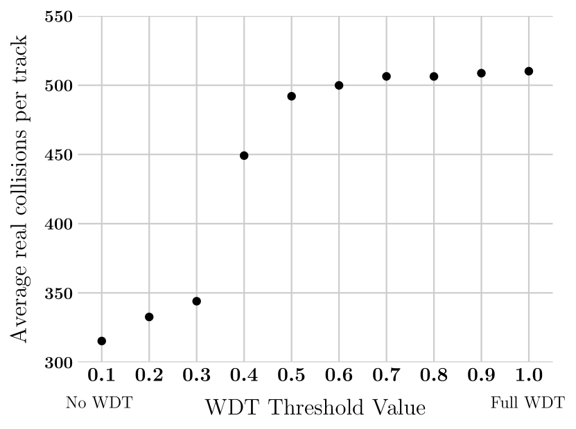
(a)

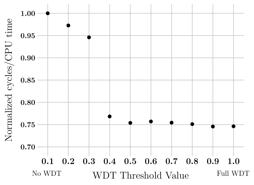
(b)

Figure 6: For the PWR reactor pin cell, (a) cycles per CPU time (normalized to the base case with no WDT) and (b) average real collisions per track, with increasing threshold to wdt, $P_{\mathrm{wdt}}$

Figure 7: Normalized cycles per CPU time for the PWR pin cell and fast reactor pin cell. Values are noramlized to the case with no WDT.

	Cycles/CPU time
$P_{\text{wdt}}$	Fast pin cell	PWR pin cell
0.1	1.00	1.00
0.2	0.98	0.97
0.3	0.95	0.95
0.4	0.88	0.77
0.5	0.82	0.75
0.6	0.77	0.76
0.7	0.74	0.75
0.8	0.74	0.75
0.9	0.74	0.75
1.0	0.67	0.75

4.3 Figure of Merit

At first glance, the WDT method appears to be less efficient by causing more real collisions, and therefore requiring more clock time for the simulation to run the same number of particles. Ultimately, though, running many particles is not the goal of the simulation. Our goal is calculating parameters of interest with low error, so this must be taken into account. Because variances are inversely proportional to the number of neutron cycles simulated with this relationship,

$$\sigma^{2}(\hat{x})=\frac{C}{n}\>.$$ (7)

where $n$ is the number of cycles and $C$ is a constant, we can theoretically always reduce the variance at the expense of more cycles and CPU time. The goal of efficient variance reduction is therefore to reduce the constant $C$, such that a smaller variance can be achieved for a given number of cycles $n$. We will describe this constant using a figure of merit (FOM).

The commonly-used formulation of this FOM is described by Lewis and Miller [1],

$$\mathrm{FOM}=\frac{1}{\sigma(\hat{x})^{2}t}\>,$$ (8)

where $t$ is the runtime of the simulation and is proportional to the number of cycles $t\propto n$. Plugging this and Eq. (7) into Eq. (8) yields:

$$\mathrm{FOM}=\frac{1}{\sigma(\hat{x})^{2}t}=\frac{n}{C_{1}}\cdot\frac{1}{C_{2}\cdot n}=C_{3}\>,$$

where $C_{1},C_{2},$ and $C_{3}$ are constants. We therefore expect the FOM to be a constant value independent of the number of cycles $n$. A higher FOM indicates lower variance per computation time, and therefore a more efficient algorithm.

A Serpent simulation was run for both test cases using values of the WDT threshold ($P_{\mathrm{wdt}}$) from 0.1 to unity in increments of 0.1, maintaining a constant threshold to ray tracing, $P_{\mathrm{ray}}$, as described in Fig. 2. We normalized the final FOM for each value of $P_{\mathrm{wdt}}$ to the final FOM with no WDT:

$$\text{FOM}_{\text{norm}}(P_{\mathrm{wdt}})=\frac{\mathrm{FOM}(P_{\mathrm{wdt}})}{{\mathrm{FOM}}_{0}}\>,$$

where ${\mathrm{FOM}}_{0}={\mathrm{FOM}}(0.1)$ is the FOM with no WDT. Increasing values of $P_{\mathrm{wdt}}$ leads to increasing the amount of WDT over regular delta-tracking. The parameters for the rouletting scheme are kept constant, with a weight cutoff of $w=0.1$ and probability of rouletting $P_{\mathrm{kill}}=0.5$.

First, all simulations were run for a long enough period for the FOM to converge. The cycles/CPU time is observed to ensure computer loading did not change. Then, the FOM at each point in the simulation is calculated using the total cycles, $C$:

$$\text{FOM}_{C}=\frac{1}{\sigma(\hat{x})^{2}C}\,.$$ (9)

Then, all connections were isolated to the cluster so that no other loading would be placed on it. We ran each of the simulations for a shorter duration (approximately two hours) to ensure a value of cycles/CPU time converged. This is then multiplied by $\text{FOM}_{C}$ to return the FOM:

$$\text{FOM}_{C}\cdot\frac{C}{t}=\frac{1}{\sigma(\hat{x})^{2}C}\cdot\frac{C}{t}=\frac{1}{\sigma(\hat{x})^{2}t}=\text{FOM}\,.$$ (10)

This process ensures that the FOM for all runs is normalized to the same computer loading.

4.4 Analysis Package

As discussed in the previous section, we want to observe the convergence behavior of the FOM to determine the final value. To do so, we modified the Serpent 2 source code to generate uniquely named output files at various cycle values. We developed the WDT_Analysis package to leverage Python’s object oriented programming structure and enable easy analysis of the data. We utilize a module, fom, to analyze the convergence of FOM across many Serpent 2 output files.

4.5 Parameters of study

Each Serpent 2 simulation generates hundreds of output parameters that describe all processes that occur during particle propagation. To focus our search, we identified two quantities that will be the focus of this study: flux and total cross-section. Further study into other parameters may reveal further benefit or issues with the WDT method. Both test cases have reflective boundary conditions, so we will examine the infinite values for the parameters of interest.

4.5.1 PWR pin cell fast group

In the PWR pin cell simulation, fast group interactions are dominated by scattering and a small amount of absorption in the light water moderator. The majorant cross-section is defined by the uranium fuel; for values of $P_{\mathrm{wdt}}<1.0$, only standard delta-tracking is used in the fuel region. Therefore, any changes in FOM are likely due to interactions in the moderator region.

The infinite flux ($\phi_{\infty}$) FOM of the fast group is shown in Fig. 8. The data show an improvement in FOM at most values of $P_{\mathrm{wdt}}\leq 0.7$. As neutrons in the fast group scatter in the moderator and lose energy, the total cross-section for absorption increases exponentially leading to a subsequent rise in $P_{\mathrm{real}}$. As discussed, the WDT routine is only used when $P_{\mathrm{real}}$ is less than or equal to $P_{\mathrm{wdt}}$. Increasing $P_{\mathrm{wdt}}$ will therefore cause more absorption events to use the WDT routine instead of standard delta-tracking. These absorption events now always contribute to the statistics of the problem, reducing variance. This correlates to the rise in average real collisions per track in Fig. 6(a). Eventually, this increase in the number of real collisions levels off for $P_{\mathrm{wdt}}>0.7$, and we see a subsequent leveling off of FOM. There is a small decrease in FOM, possibly due to the inefficiency of using WDT compared to delta-tracking in high scattering regions.

PWR fast group $\phi_{\infty}$

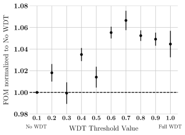
Figure 8: FOM for the PWR infinite flux $\phi_{\infty}$ for the fast group. Error bars shown are one standard deviation.

The infinite total cross-section ($\Sigma_{\mathrm{tot,\infty}}$) FOM of the fast group is shown in Fig. 9. The reduction in FOM from the base case mimics the pattern of the cycles per CPU time seen in Fig. 6(b). This may occur because scattering is the dominant contribution to the total cross-section. Thus, the collection of more statistics for absorption events is overshadowed by the inefficiencies in scattering. By not improving the variance significantly, the driving factor in FOM becomes the cycles per CPU time.

PWR fast group $\Sigma_{t,\infty}$

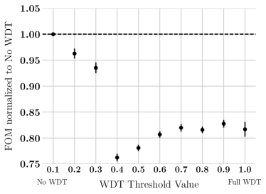
Figure 9: FOM for the PWR infinite total cross-section $\Sigma_{t,\infty}$ for the fast group. Error bars shown are one standard deviation.

4.5.2 PWR pin cell thermal group

The thermal group interactions in the PWR pin cell simulation are dominated by absorption, with very little scattering. For the infinite flux, shown in Fig. 10 we see a consistent improvement in the FOM with increasing $P_{\mathrm{wdt}}$. The improved statistics provided by the increased number of real collisions outweighs the computational inefficiency of the increased tallying required.

PWR thermal group $\phi_{\infty}$

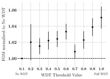
Figure 10: FOM for the PWR infinite flux $\phi_{\infty}$ for the thermal group. Error bars shown are one standard deviation.

The infinite total cross-section for the PWR pin cell thermal group is shown in Fig. 11. The trend here is less consistent than in the other plots. There is a clear increase in FOM at a $P_{\mathrm{wdt}}$ value of unity, the only value where collisions in the fuel use WDT. The fuel region dominates the absorption events for thermal neutrons, so the improved statistics leads to a higher FOM. Ignoring that point, we see a rise and fall in FOM improvement, with a peak at $P_{\mathrm{wdt}}=0.7$. Unlike the fast group, the total cross-section is dominated by absorption, so the increased number of real absorption events clearly improves the FOM. This improvement may not be great enough to overcome the inefficiency introduced with more WDT.

PWR thermal group $\Sigma_{t,\infty}$

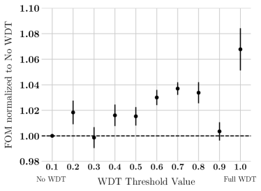
Figure 11: FOM for the PWR infinite total cross-section $\Sigma_{t,\infty}$ for the thermal group. Error bars shown are one standard deviation.

4.5.3 Fast reactor pin cell fast group

In the fast reactor pin cell, the fast neutron group drives fission and therefore dominates absorption reactions. Like the PWR pin cell, the majorant cross-section is defined by the MOX fuel. Changes in FOM are therefore likely due to interactions in the lead coolant and cladding. Lead has a very low absorption cross-section for fast neutrons, so much of the FOM change will be driven by absorption in the cladding.

The infinite flux for the fast reactor pin cell is shown in Fig. 12. We observe a rise in FOM as more WDT is introduced and more absorption events contribute to the overall statistics. Eventually, the improvement in statistics is overcome by the inefficiency of introducing many more real collisions, and the improvement decreases. When WDT is introduced in the fuel, at $P_{\mathrm{wdt}}$ of unity we see a large decrease in FOM, which matches the drop in cycles/CPU time at the same value.

Fast reactor pin cell fast group $\phi_{\infty}$

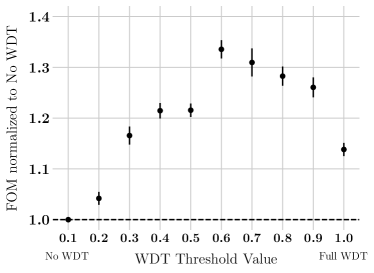
Figure 12: FOM for the fast reactor infinite flux $\phi_{\infty}$ for the fast group. Error bars shown are one standard deviation.

A similar pattern is seen in the infinite total cross-section, shown in Fig. 13. Again, we observe a rise in FOM concurrent with the introduction of WDT, as more absorption events are contributing to the statistics. We see an uncharacteristic drop at $P_{\mathrm{wdt}}=0.7$ that does not seem to fit the overall pattern. Further simulation and exploration is required to determine the cause of this outlier.

Fast reactor pin cell fast group $\Sigma_{t}$

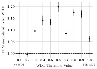
Figure 13: FOM for the fast reactor infinite total cross-section $\Sigma_{t}$ for the fast group. Error bars shown are one standard deviation.

4.6 Choice of WDT threshold

As we see in the two test cases, use of the WDT with scattering routine results in an observable change in FOM in the infinite flux and infinite total cross-section. Although the cycles per CPU time is negatively impacted by WDT for both test cases, the collection of more statistics results in more efficient simulations, as measured by FOM.

For the PWR simulation, WDT results in a small improvement in the FOM for both group infinite fluxes, and the thermal group infinite total cross-section. Therefore, for simulations seeking accurate flux and thermal cross-sections, the data suggest that full WDT with scattering ($P_{\mathrm{wdt}}=1$) would result in the largest improvement. This improvement is driven by the use of the WDT routine in the fuel region, where WDT only turns on when $P_{\mathrm{wdt}}=1$ in our test cases. In simulations with heavy absorbers where the fuel region does not define the majorant cross-section, the same results may not be observed. In those cases, a lower value of WDT threshold will be sufficient to enable the WDT routine in the fuel regions.

Use of WDT with scattering also generates an observed increase in FOM for the fast reactor pin cell. The results differ from the PWR in two significant ways. First, the improvement is not maximized at a threshold value of unity. Instead, improvement in FOM for the infinite flux and total cross-section peaks when $P_{\mathrm{wdt}}=0.6$ and then declines. Second, the improvement is of a much higher magnitude, reaching an improvement of nearly 20% and over 30% for the infinite cross-section and flux, respectively. This is much more significant than the sub-ten percent improvement for the PWR pin cell. Therefore, the data suggest that for a fast pin cell simulation, mid-range value of WDT threshold may result in the greatest improvement in FOM.

A summary of all the relative FOM values and the associated error are shown in Table 14.

Figure 14: FOM as a function of $P_{\text{wdt}}$ for the PWR and fast reactor pin cell, noramlized to the no-WDT case of $P_{\text{wdt}}=0.1$.

	PWR				Fast Reactor
	Fast group		Thermal group		Fast group
$P_{\text{wdt}}$	$\phi_{\infty}$	$\Sigma_{t,\infty}$	$\phi_{\infty}$	$\Sigma_{t,\infty}$	$\phi_{\infty}$	$\Sigma_{t,\infty}$
0.1	1.000 $\pm$ 0.000	1.000 $\pm$ 0.000	1.000 $\pm$ 0.000	1.000 $\pm$ 0.000	1.000 $\pm$ 0.000	1.000 $\pm$ 0.000
0.2	1.018 $\pm$ 0.008	0.963 $\pm$ 0.010	1.020 $\pm$ 0.022	1.018 $\pm$ 0.009	1.042 $\pm$ 0.013	0.995 $\pm$ 0.009
0.3	0.999 $\pm$ 0.010	0.935 $\pm$ 0.010	1.015 $\pm$ 0.010	0.999 $\pm$ 0.008	1.166 $\pm$ 0.018	1.095 $\pm$ 0.014
0.4	1.035 $\pm$ 0.006	0.762 $\pm$ 0.007	1.022 $\pm$ 0.011	1.016 $\pm$ 0.008	1.217 $\pm$ 0.015	1.140 $\pm$ 0.019
0.5	1.014 $\pm$ 0.010	0.781 $\pm$ 0.006	1.024 $\pm$ 0.010	1.015 $\pm$ 0.007	1.216 $\pm$ 0.013	1.132 $\pm$ 0.013
0.6	1.055 $\pm$ 0.005	0.807 $\pm$ 0.006	1.033 $\pm$ 0.010	1.030 $\pm$ 0.006	1.335 $\pm$ 0.018	1.198 $\pm$ 0.023
0.7	1.066 $\pm$ 0.009	0.820 $\pm$ 0.007	1.008 $\pm$ 0.009	1.037 $\pm$ 0.005	1.310 $\pm$ 0.028	1.084 $\pm$ 0.018
0.8	1.052 $\pm$ 0.005	0.816 $\pm$ 0.006	1.023 $\pm$ 0.011	1.034 $\pm$ 0.008	1.283 $\pm$ 0.019	1.175 $\pm$ 0.014
0.9	1.049 $\pm$ 0.006	0.827 $\pm$ 0.007	1.039 $\pm$ 0.011	1.003 $\pm$ 0.007	1.261 $\pm$ 0.020	1.168 $\pm$ 0.015
1.0	1.045 $\pm$ 0.012	0.817 $\pm$ 0.014	1.051 $\pm$ 0.013	1.068 $\pm$ 0.017	1.138 $\pm$ 0.013	1.062 $\pm$ 0.013

5 Conclusion

In this work, we described the delta-tracking technique and the more recent WDT method that seeks to improve it. We then described the issues with extending the WDT to include scattering, and introduced a novel hybrid modification. We implemented the method in the Serpent 2 Monte Carlo code and examined the results of simulations with two test cases. We then compared the FOM for two simulation results against the base case to determine the impact of varying the threshold at which WDT with scattering is used.

Based on these results, we can conclude that the WDT routine with scattering does modestly improve FOM in infinite flux for the PWR and fast reactor pin cells. For total cross-section, FOM is similarly improved, except in the fast group for the PWR pin cell. In both cases, the WDT with scattering routine reduces cycles per CPU time, by increasing the number of simulated real collisions for absorption events. We hypothesize that this increased number of real absorption events is the main driver in improving FOM.

Further study should look into possible synergy or issues with use of the WDT with scattering routine and other variance reduction techniques, such as implicit capture.

Based on the findings of Legrady et al.[6], we expect an improved hybrid method could be developed that combines sampling cross-sections not explored here. Extension of their method in a highly scattering region may result in a similar multiplication of particles, with a different splitting of weights. A hybrid method that uses their optimized sampling cross-section for non-scattering events, and normal delta-tracking for scattering events may result in significant improvement over the method described here.

In addition, a finer resolution in threshold values may provide a clearer relationship between the amount of WDT and improvement in FOM. Finally, we hypothesize that the impact of WDT on FOM will be very different in simulations where the fuel region does not define the majorant cross-section. Further study should look at test problems with heavy absorbers that drive majorant cross-section.

6 Acknowledgments

This article was prepared by J.S. Rehak under award NRC-HQ-84-14-G-0042 from the Nuclear Regulatory Commission. The statements, finding, conclusions, and recommendations are those of the author(s) and do not necessarily reflect the view of the US Nuclear Regulatory Commission.

7 References

References

- [1] E. E. Lewis and W.F. Miller, Jr. Computational Methods of Neutron Transport. American Nuclear Society, 1993.
- [2] J. Leppänen. Development of a New Monte Carlo Reactor Physics Code. PhD thesis, Helsinki University of Technology, 2007.
- [3] Jaakko Leppänen. Performance of Woodcock delta-tracking in lattice physics applications using the Serpent Monte Carlo reactor physics burnup calculation code. Annals of Nuclear Energy, 37:715–722, 2010.
- [4] Jaakko Leppänen. Modeling of Nonuniform Density Distributions in the Serpent 2 Monte Carlo Code. Nuclear Science and Engineering, 174:318–325, 2013.
- [5] Jaakko Leppänen. Serpent – A Continuous-energy Monte Carlo Reactor Physics Burnup Calculation Code – User’s Manual, June 2015.
- [6] D Legrady, B Molnar, M Klausz, and T Major. Woodcock tracking with arbitrary sampling cross section using negative weights. Annals of Nuclear Energy, 102:116–123, 2017.
- [7] Iván Lux and László Koblinger. Monte Carlo Particle Transport Methods: Neutron and Photon Calculations. CRC Press, 1991.
- [8] L.W.G. Morgan and D. Kotlyar. Weighted-delta-tracking for Monte Carlo particle transport. Annals of Nuclear Energy, 85:1184–1188, 2015.
- [9] N. Metropolis and S. Ulam. The Monte Carlo Method. Journal of the American Statistical Association, 44(247):335–341, 1949.
- [10] J. Ortensi et al. Updates to the Generation of Physics Data Inputs for MAMMOTH Simulations of the Transient Reactor Test Facility. Technical Report INL/EXT-16-39120, Idaho National Laboratory, June 2016.
- [11] VTT Technical Research Centre of Finland. VTT Serpent. http://montecarlo.vtt.fi/. Accessed: 2017 April 18.
- [12] E.R. Woodcock et al. Techniques used in the GEM code for Monte Carlo neutronics calculations in reactors and other systems of complex geometry. ANL-7050. Argonne National Laboratory., 1965.