Cyberhubs: Virtual Research Environments for Astronomy

Abstract

Collaborations in astronomy and astrophysics are faced with numerous cyber infrastructure challenges, such as large data sets, the need to combine heterogeneous data sets, and the challenge to effectively collaborate on those large, heterogeneous data sets with significant processing requirements and complex science software tools. The cyberhubs system is an easy-to-deploy package for small to medium-sized collaborations based on the Jupyter and Docker technology, that allows web-browser enabled, remote, interactive analytic access to shared data. It offers an initial step to address these challenges. The features and deployment steps of the system are described, as well as the requirements collection through an account of the different approaches to data structuring, handling and available analytic tools for the NuGrid and PPMstar collaborations. NuGrid is an international collaboration that creates stellar evolution and explosion physics and nucleosynthesis simulation data. The PPMstar collaboration performs large-scale 3D stellar hydrodynamics simulation of interior convection in the late phases of stellar evolution. Examples of science that is presently performed on cyberhubs, in the areas 3D stellar hydrodynamic simulations, stellar evolution and nucleosynthesis and Galactic chemical evolution, are presented.

published date

1 Introduction

New astronomical observatories, large surveys, and the latest generation of astrophysics simulation data sets, provide the opportunity to advance our understanding of the universe profoundly. However, the sheer size and complexity of the new data sets dictate rethinking of the current data analytic practice which can often be a barrier to fully exploiting the scientific potential of these large data sets. The following challenges may be identified.

The typical size of data sets in astronomy & astrophysics continues to grow substantially. To name a few examples, optical waveband projects such as the Large Synoptic Survey Telescope (LSST), radio facilities such as the Square Kilometer Array (SKA) pathfinders, as well as large data sets produced by cosmological or stellar hydrodynamics simulations which will, in combination, produce 10s of petabytes of scientific data that would not typically be held in one place. Such data sets can not be downloaded for processing and analysis. Instead combining remote computer processing capacity where the data is stored with the appropriate analytic and data processing software stacks is required. On top of that efficient remote access with visualization and interaction capabilities are needed to enable a distributed community to collectively explore these data sets. Instead of moving the data to the processing machines, the processing pipelines need to be moved to where the data resides.

One of the great promises of the age of data science for astronomy is that the many multi-physics, multi-messenger, multi-wavelength and multi-epoch constraints that bear on most problems in astronomy, can in fact be combined successfully when complex data interactions and collaborative cyber-research environments are constructed. This notion of data fusion between different types of observational data and simulation data can reach its full potential when different communities can come together in combining and sharing data sets, analytical tools and pipelines, and derived results.

A significant barrier in accomplishing this goal in practice are authentication and access models. Resources are often provided by national bodies or consortia with often burdensome access requirements and limitations. An effective research platform system would accept easily-available social or otherwise broadly used third-party identities to allow flexible, international, collaborative access. Although single sign-on technologies are emerging, the scientific community is still far from adopting them.

Decades worth of investments in legacy software, tools, and workflows by many research groups may be lost and never shared with a broader community or applied to new data sets. The reproducibility of science is suffering when data processing and analytic workflows can not be shared. A modern research platform would provide a uniform execution environment that will liberate legacy software, unlocking its analytic value and that of associated data sets, making them available to others, and allowing them to reproducibly interact with analysis procedures and data sets of other researchers.

In this paper we describe cyberhubs, an easily-deployed service that combines Juypter notebook or Jupyterlab data and processing in a containerized environment with a prescribed software application toolbox and data collection. The system described here is the result of multi-year developments and evolution, with the goal to address the limitations and challenges, initially of the international NuGrid collaboration, and then in addition, those of the PPMstar collaboration. Both of these brought somewhat different demands and requirements, that in combination are likely typical for a very wide range of use cases in astronomy and astrophysics.

The international Nuclesoynthesis Grid (NuGrid) collaboration has members from $\approx 20$ institutions in many countries (Pignatari & Herwig, 2012). Since 2007, NuGrid has been combining the required expertise from many different scientists to generate the most comprehensive data sets for the production of the elements in massive and low-mass stars to date (Pignatari et al., 2016; Ritter et al., 2017b). Around 2009, when the first data set was created it had a size of $\approx 5\;\mathrm{TB}$, which is relatively small by today’s standards, however still large enough that it is not easily transferred around the globe on demand. The collaboration was faced with problems that are common to any distributed, data-oriented collaboration. Problem-specific processing and analytic tools are developed, but deployment in different places is always complicated by a diverse set of computing environments. In the NuGrid collaboration, which brings together different communities, all of the three major operating systems are used. Initially, three copies of the data sets were always maintained at three institutions in the UK, Switzerland and Canada through a tedious, time-consuming and error-prone syncing system. Still, analytic and interactive access for researchers who were not at one of those three institutions was very limited through VNC sessions or X11 forwarding, and required account-level access sharing that would be probably impossible at most institutions today.

As a next step, the collaboration adopted CANFAR’s VOspace as a shared and mountable storage system. CANFAR is the Canadian Advanced Network for Astronomy Research, a consortium between NRC (National Research Council) Herzberg’s Canadian Astronomy Data Center (CADC) and Canadian university groups which aims to jointly address astronomy cyber-infrastructure challenges. VOspace provides shareable user storage with a web interface, and identity and group management system, similar to commercial cloud storage systems such as Google Drive and Dropbox. It also has a Python API vos that allows command line access to VOspace and POSIX mounting to a local laptop or workstation. The mounting option, in particular, made VOspace very promising for the collaboration, as it allows for the replacement of three distributed storage copies with just one master copy, which can be mounted from anywhere. In addition, it includes a smart indexing algorithm which ensures that only the data needed for an analysis or plot is transferred. Although this system was a significant improvement, it did not work for remotely executed analysis projects requiring high data throughput of most of the available data set, and it did not solve the problem that many in the collaboration felt restricted by complications in establishing and maintaining the NuGrid software stack. This software stack is not particularly complex, from the viewpoint of a computationally experienced user, but in order to address the diverse set of science challenges, the collaboration includes members that deploy a diverse set of science methodologies, and especially entry-level researchers and researchers-in-training have often found establishing and maintaining the NuGrid software stack to be a substantial barrier.

We tried to overcome this challenge by using virtual machines based on Oracle’s VirtualBox technology. We have, for example, developed VMs for the Nova project, which is admittedly now mostly defunct. While in principle VMs allow one to load a pre-defined software stack into a VM as well as the VOspace access tools, in practice, this technology has not been adopted broadly. The reasons for that were a combination of rather time-consuming and ridged maintenance requirements and reports of usability issues. In addition to their heavy weight nature, the VMs also did not properly address the need for distributed teams to collaborate on the same project space, because they limit any VM instance to only one researcher.

From the beginning in 2007, the NuGrid collaboration had adopted Python as the common analytic language. Around 2012/2013 the ipython notebook technology became increasingly popular in the collaboration. In collaboration with CANFAR, we developed as one of two applications of the project Software-as-a-Service for Big Data Analytics funded by Canarie the Web-Exploration for Nugrid Data Interactive (WENDI Jones et al., 2014) service, which had some of the functionality that is now offered by JupyterHub. This project was very successful in establishing a prototype for web-enabled analytic remote data access with a pre-defined, stable analytic software stack and network proximity to the data for a fast and interactive, remote data exploration experience. For some years NuGrid served graphical user-interfaces built on ipywidgets of the SYGMA and OMEGA tools of the NuGrid Python Chemical Evolution Environment (NuPyCEE, Ritter & Côté, 2016) as well as the NuGridSetExplorer which allows GUI access to the NuGrid stellar evolution and yield data sets (Pignatari et al., 2016; Ritter et al., 2017b). The project was to a large extent focused on improvements to the storage backend, enabling for example VOspace to work well with indexed hdf5 files, and thus did not add authentication and access management to the service. The usage was therefore limited to anonymous and time-limited access. The service was deployed on virtual machines of the Compute Canada cloud service.

Another set of requirements for the cyberhubs facility presented here originates from a stream of efforts in providing enhanced data access within a collaboration, and ultimately to external users, undertaken by the PPMstar collaboration (Woodward et al., 2015; Herwig et al., 2014). The typical size of the aggregate data volume for a single project involving three-dimensional stellar hydrodynamics simulations is $\approx 200\;\mathrm{TB}$, and the collaboration would at any given time work simultaneously on two to three projects. The simulations are performed at super-computing centers, such as the NSF’s Blue Waters computer at the NCSA in Illinois, or high-performance computing facilities in Canada, such as WestGrid’s orcinus cluster at UBC or the cedar cluster at SFU. Blue Waters has relatively restrictive access requirements which make it somewhat burdensome to add international collaborators to access the data, especially temporary access for students. For interactive access or processing access by collaboration members who cannot login to Blue Waters, data has to be moved off the machine, which is not practical since such external collaboration members do not have the required storage facilities, and the network bandwidth is insufficient. In addition, over decades the LCSE has developed custom and highly optimized software tools to visualize and analyse the algorithmically compressed data outputs of the PPMstar codes. More recently, new tools have been developed using Python. The data exploration and analysis ecosystem of the collaboration is heterogeneous and difficult to maintain even for core members in view of the constantly changing computing environments on the big clusters and the home institutions. The challenge for this collaboration was to stabilize and ease the use of legacy software, the very large data volumes and the access and authentication when trying to broaden the group of users that can have analytic and exploratory access to these large and valuable data sets.

Based on these requirements, and through experience, we have combined the latest technologies, including Docker and Jupyter and designed cyberhubs, a system that allows easy deployment of a customized virtual research environment (VRE). It offers flexible user access management, and provides mechanisms to combine the research area specific software applications and analytic tools with data and processing to serve the needs of a medium-sized collaboration or user group. At a larger scale, an architecture similar to cyberhubs has been deployed, for example, by the NOAO in their NOAO data lab, and has been selected for the LSST Science Platform. JupyterHub-based systems are also used in teaching large data science classes, such as the UC Berkeley Foundations of Data Science course. At the University of Victoria a precursor of the architecture described here has been used in both graduate and undergraduate classes for the past three years. Another broad installation of this type is the Syzygy project that allows institutional single-sign-on to Jupyter Notebook servers across many Canadian universities to access Compute Canada resources.

cyberhubs, although scaleable in the future, is at this point addressing the needs of medium-sized collaborations which require an easy to setup and maintain shared research environment. The cyberhubs software stack is available on GitHub and the docker images are available on Docker Hub. In §2 we describe the system architecture and implementation, in §3 we briefly sketch the typical steps involved in deploying cyberhubs, and in §4 we present the two main deployed applications and how to add new applications. We close the paper with some discussion of limitations and future developments in §5.

2 System architecture and implementation

In this section we describe the architecture and design features as well as the implementation of cyberhubs. Here, a cyberhub administrator configures and deploys the service, while a cyberhub user is simply someone who connects to the deployed service, and is not burdened with the details described here.

2.1 General design features

To satisfy the requirements of the cyberhubs system, we combine the following components:

1. A thin user interface component allows the users to easily interact with their virtual research environment (VRE).

2. The authentication component ensures the right researchers are accessing the proper data, processing and software analytic tools in their VRE.

3. The docker spawner component that allows the users to spawn their selected choice of application containers and allows selection of Jupyter environment (notebook or lab).

4. The image repository offers prebuilt container images for all components and can be expanded to host new VREs for other applications.

5. The notebook templates and interactive environments help the users to get started in their VREs and preparing their own analytic workflow.

6. A deployment component enables administrators, such as the data infrastructure experts in a collaboration, to deploy all of the above components with minimal effort and customization.

The first three components are offered by JupyterHub, with some modifications we made to the second one to allow dynamic white and black listing for user management. The fourth is partially enabled by the Cyberhubs Docker Hub repository. The fifth and sixth components, and the customization images are offered by cyberhubs.

cyberhubs provides a complete, packaged system that can easily be installed and customized and allows the cyberhubs administrator to quickly deploy VREs. There is no reason why a particular cyberhubs instance could not be near-permanent, with little in maintenance needed because the system is based on docker images. However, the cyberhubs system is designed for easy deployment with all essential configuration options, like attaching local or remote storage volumes, provided through external configuration files that then will be absorbed by the pre-built docker images.

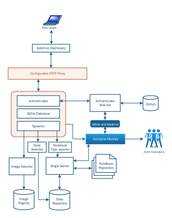
Figure 1: cyberhubs general system architecture.

As opposed to other packaging solutions that rely on tools such as ansible, puppet and others, cyberhubs requires only setting a minimal number of environment variables to deploy any of the pre-built application hubs which could possibly enable many astronomy use cases. Extending an application hub, or building a new one on top of corehub (part of cyberhubs repository) is straight forward and well documented. An example if the application SuperAstroHub (available in the Cyberhubs Docker repository) available on the WENDI server (see §4.1.1) that combines all of our presently available cyberhub applications.

The general system architecture for the cyberhubs is shown in Fig. 1. JupyterHub is a multi-user environment that allows the users to authenticate and launch their own notebook and terminal server, while sharing access to certain storage areas. By doing so, the same collaboration infrastructure can be used by multiple users and therefore provide a platform for sharing resources, analytic tools, as well as research content and outcomes. The main components of JupyterHub are:

• A configurable HTTP proxy that allows the users to interact with the system and directs their requests to the appropriate service.

• A hub that handles users and their notebooks. In more detail, the hub offers the following services:

  • An authentication service that supports many authentication backends (including PAM, LDAP, OAuth, etc.). Currently, cyberhubs uses an extended Github authenticator that allows users with GitHub account to log into cyberhubs.

  • A spawner service that allows the user to select the singleuser application hub and the interface type.

  • An SQLite database which keeps track of the users and the state of the hub.

2.2 Spawner and authentication extensions

Our extended spawner is integrated in the JupyterHub configuration file. It provides at this point two selection options. First the user selects between the default Jupyter Notebook option and the experimental option JupyterLab. Both JupyterLab and Notebooks offer Python, bash and other language notebook options as well as terminal access to the singleuser hub container. JupyterLab is a significantly enhanced Jupyter interface that overcomes the restrictions imposed by single linear notebooks or terminals, and allows one to combine multiple sessions in parallel in one web browser window. For the second option, the user can select the application hub image if multiple options are configured to be offered by the cyberhubs administrator. In the future a simple extension could allow one to choose between a variety of data access options in this spawner menu.

A major challenge in a shared environment is access and authentication administration. For most collaborations, national or institutional authentication models are not practical. We have adopted the third-party OAuth authentication method available for JupyterHub and allow authentication of users with their GitHub accounts. Other third-party OAuth applications, such as Google, could be used as well.

To dynamically control the GitHub users who can access the system, our authentication extension provides a simple whitelist and blacklist mechanism that can be updated in the running, fully deployed cyberhubs without service interruption. The authenticator relies on a whitelist and/or blacklist file to dynamically grant or deny access to GitHub users. When a whitelist is supplied, only the users in that list are allowed to login. When the blacklist is present, the users in the blacklist are blocked from accessing the system and will get a 403: forbidden page even if they are in the whitelist.

This is a rather simple yet powerful access model that allows, in combination with the easy configuration of the storage additions to the cyberhubs, a flexible access control to data and processing that can serve in a flexible way the access and sharing requirements of medium-sized collaborations. It can be easily combined with temporary unrestricted access to any user.

Unlike some JupyterHub installations that propagate the host system identity to the hub user, or systems that create inside the singleuser application container an identity according to the login identity, we are adopting a simpler approach with the goal of enabling the most transparent and seamless sharing and collaboration. In cyberhubs all users have in their own application hub container the identity user. Typically, a read-write data volume of considerable size is attached, and all users appear as users on that read-write volume with the same identity.

Another major component in a shared environment is resource allocation. By resources we are referring to cpu, memory, swap space and disk storage. Currently, we are not enforcing any resource limits and we are not offering any scheduling capabilities. We are considering to add the abilities to specify resource limits for every container launched and to alert users if no more resources are available. Since these abilities do not ensure a scalable system, our roadmap includes a plan to use Docker Swarm and/or Kubernetes for scaling the resources and scheduling the containers.

2.3 Features and capabilties

Both Jupyter Notebook and Jupyterlab offer web-based notebook user interfaces for more than 50 programming languages, and we included by default python 2 and 3 and bash. But other popular languages, such as R or Fortran are easily added. Both bash notebooks as well as terminals provide shell access to the singleuser application docker container (that we call here hub). Any simulation or processing software that can be executed on the Linux command line, such as the MESA stellar evolution code (Paxton et al., 2010, 2013, 2015) or the NuGrid simulations codes (Pignatari et al., 2016), can be run by each user in their identical instance on the full hardware available on the host. Other examples include legacy analysis and processing tools that require a special software stack. If such software is once expressed in the singleuser application hub docker image it can be easily shared with anyone accessing the cyberhubs.

cyberhubs are typically configured with an openly shared, trusted user space that is equally available to all users that have access to a particular cyberhub. This user space is mounted on a separate, persistent volume. A trusted collaboration, would establish some common sense rules on how to access this shared space, in which all participants have seamless access to any project or individual directories. We have found that this arrangement allows for very effective cooperation between team members with very different skill sets, including students.

A typically small amount of private non-persistent storage is available inside the user’s singleuser hub instance, which will disappear when the user container is restarted. In order to create some level of persistence beyond the shared user space, users of cyberhubs rely heavily on external, remote repositories, such as git repositories, for storing and sharing non-data resources, such as software, tools, workflows, documentation, and paper writing manuscripts.

In addition to analytic access to data the cyberhubs provide documentation and report writing through inline Markdown cells, a latex typesetting environment where pdf files are seamlessly viewed in the browser for paper manuscript writing and editing, as well as slide presentation extensions to Jupyter which allow one to create presentations with live plots and animations. In addition, graphical user-interface applications can be built, and examples are provided in wendihub (§4.1.1).

In terms of the maintenance of the multiuser environment, where many containers are running, the cyberhubs administrator should monitor the state of the cyberhub, including the available resources. Astray and blacklisted user containers should be removed.

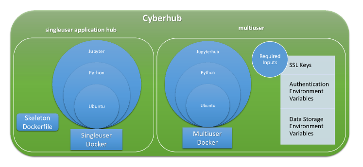
Figure 2: Main elements of the core cyberhubs system. The multiuser takes care of receiving the initial service request from a user, handles user authentication and and data storage attachment. It launches a singleuser application hub from the appropriate image or reconnects a returning user to that user’s existing application container. The singleuser component contains the application-specific analytic software and is the processing home for the user. Each user has a separate container instance of the application image.

A typical cyberhub includes a repository of examples and template notebooks to help users getting started in exploring the data resource. These notebooks can be copied into the image or provided via mounted volumes. Each cyberhub in our cyberhubs family has strict version-specific requirements files for python and Linux packages, that ensure that the same versions of each component of the entire software stack are always used, until an update is made. In that case, past docker image versions will be still available as tagged images on the docker hub repository. Each user has therefore a completely controlled and reproducible environment. It is then straight-forward to create a stable, shareable and reproducible science workflow. Simulation software and analysis packages are shared via repository platforms such as GitHub, GitLab or BitBucket, and include information on exactly which cyberhub  including the version, it is to be deployed.

At the core of the cyberhubs design is the multiuser image and a basic corehub singleuser application. The latter is a skeleton and has no application software installed. The main elements of these core elements of cyberhubs are shown in Fig. 2. They are:

1. multiuser image: It is composed of our customized JupyterHub image, available via dockerhub repository, or via build package that includes Dockerfile and all other necessary scripts and docker-related files to customize, compose and then launch the multiuser JupyterHub service.

2. singleuser corehub image: The most basic, bare singleuser docker image, also available via dockerhub repository or build package.

corehub is the starting point on top of which all of the other application hubs are built (§3), as shown in Fig. 3. Obviously, not only astronomy cyberhubs can be built on top of corehub, but applications from other disciplines or use case are possible. The astronomy application hubs are the astrohubs.

2.4 Storage staging

Docker containers typically do not have much storage, and a few options of storage staging are typically deployed:

• Read-only data volume: Most cyberhubs are about providing access to a particular data universe. This is immutable data that is staged on read-only data volumes. It is mounted on the singleuser container to allow the users to read the data in their notebooks and processing as needed.

• Persistent data volume: This volume is also mounted and all users have the ability to write to and read from it. The volume lives on the host or externally attached storage, and is protected against singleuser container shutdowns.

• Local ephemeral storage: This is the local storage allocated to each container when created. It is available to the users only when the container is running and gets purged once the container is removed. This holds a copy of example notebooks added to the image to be available to all users. This it the home directory of each user. Since this area is inaccessible to other users of the cyberhub it is the right place to store, for example, a .gitconfig file or other configuration files as well as a .ssh directory.

• Individual remote data storage: Users can use sshfs, mountvos, google-drive-ocamlfuse, and other fuse tools to mount their remote data storage. This, however, requires elevated privileges for the containers and is not yet supported.

Currently, read-only and persistent data volumes are specified via environment variables, and we do not support individual remote data storage yet. However, the cyberhubs administrator can now configure both read-only and persistent data volumes as remote data volumes, an option that already would serve the needs of many collaborations. We are considering to add a data selector that allows users to select volumes to mount that they have privilege for.

3 System Deployments

The goal of cyberhubs is to make deployment as easy as possible, and there are two deployment options. cyberhubs is based on dockers whose images are created and stored in a repository either locally, or on the Docker Hub repository. A Docker container is an instance of a Docker image. A cyberhub deployment always consists of two Docker containers (Fig. 2). One is an instance of the cyberhubs/multiuser image, the other is one container per user of one application hub image, such as cyberhubs/corehub. A particular configuration may choose to offer users more than one application image in the spawner menu dialogue after login, such as those offered in the cyberhubs family.

For ease of use, the first deployment option is recommended. It involves launching containers as instances from the images available in the cyberhubs organization at https://hub.docker.com/u/cyberhubs which allows deployment of a cyberhub without building any docker images. The only requirement is one must prepare the host machine and the cyberhub configuration file and launch.

The second option is for the administrator to build one or several of the required Docker images using the Dockerfile and configuration files provided. This involves building the singleuser application hub on top of one of the provided application hub images. This option allows the administrator to add features and software otherwise not available by default, and to provide specialized configurations.

For specializations that require fundamentally different data access or different user authentication models, it may be necessary to rebuild the multiuser image.

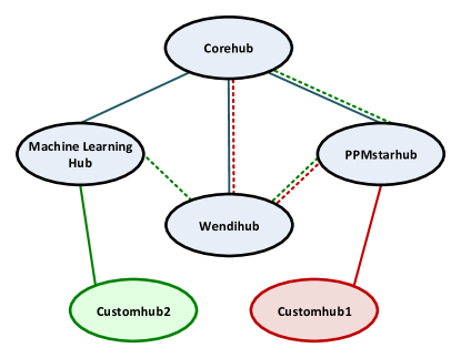
Figure 3: cyberhubs administrators can build application images by chaining existing application images and adding customization through dockerfile-based builds. By starting from the pre-built PPMstarhub that is itself based on Codehub one can build in sequential steps Wendihub and Machine Learning Hub each on top of the previous. At this point the capabilities and analytic tools of three application hubs are combined, and can be the bases for another addition of tools and data stores to create Customhub2. Similarly, for example, Customhub1 can be built as a combination of Corehub, Wendihub and PPMstarhub.

In any case the administrator follows the step-by-step documentation in the cyberhubs repository on GitHub. A deployment would involve the following steps:

• Preparing the host machine:

  • Select a host machine, such as a Linux workstation. In our case cyberhubs are deployed in a cloud environment, such as the Compute Canada Cloud, and require launching a suitable virtual machine, attaching external storage volumes, and assigning IPs. We use a CentOS7 image, but other Linux variants should work as well.

  • The host machine only needs a few additional packages, most important of which is the docker-ce package. A small amount of docker configuration is followed by launching the docker service on the host machine.

  • Any external data volumes to be made available need to be mounted. sshfs mounted volumes work well.

• Configuring the cyberhubs. This invariably starts with pulling the cyberhubs Github repo. The main steps that always must be done are:

  • Register an OAuth authentication application with a GitHub account and enter the callback address, authentication ID and secret into the single configuration file jupyter-config-script.sh.

  • Specify the admin user IDs as well as white-listed users. If white-listed users are specified, either in the configuration file (static white listing) or in the access/wlist file (dynamic white listing), then only white listed users are allowed. Otherwise everybody with a github account can have access. Dynamic black listing is also possible once the service runs.

  • Specify or modify data storage mapping from the host to the cyberhub as the user sees it, for both read-write and read-only storage.

  • Specify the application hub name. Either a single application hub is offered or the spawner menu can offer a number of different application hubs.

  • Finally, create SSL key/certificates as described in multiuser/SSL/README. While a commercial certificate can certainly be used, our default installation includes letsencrypt which provides free three-month certificates. Such certificates can be created and updated using the docker blacklabelops/letsencrypt. However, the present instructions recommend the use of certbot-auto which works well for our reference host system CentOS.

  • Source the config file and launch the cyberhub according to the instructions in multiuser/README.

• The above assumes a deployment from the pre-built docker images. This is the recommended mode. By default, the multiuser image will be automatically pulled from the repository during the execution of the docker-compose up command. However, the singleuser application hub will have to be pulled manually using the docker pull command. In addition to the basic corehub application there are several pre-built applications available in the docker hub repository, such as WENDI for NuGrid data analysis, mesahub for MESA stellar evolution, for machine learning hub mlhub to be used, for example, by StarNet (Fabbro et al., 2017), PPMstarhub for PPMstar stellar hydro data analysis.

• To add more application functionality, packages, tools, etc. it is necessary to rebuild the singleuser application hub. The Docker and configuration files of all of the existing application hubs available on Docker Hub are in the astrohubs GitHub repository. All of these application hubs start with the cyberhubs/corehub image, as indicated in the first line of the Dockerfile: FROM cyberhubs/corehub. Building or extending an application hub could start from one of the existing hubs, or from corehub. Within the cyberhubs family, all application hubs can be combined with all others. This is shown schematically in Fig. 3. In principle a super-application hub can be built by daisy-chaining all other application hubs together, collecting and adding in the process the capabilities from each participating application hub. If the community builds application hubs that are consistent with the cyberhubs model, they could be added to the cyberhubs docker hub repository.

• The multiuser image and all application hub images can also be built from scratch using the dockerfiles and configuration files provided in the GitHub repositories, starting with Ubuntu images. This allows full customization of all components, or improvements of the cyberhubs facility. The complete rebuild of the docker images would also be required when an update of the software stack is needed.

4 Applications

In this section we describe the application hubs we have built and deployed. Due to our research areas, these enable simulation-based data exploration. Applications for observationally-oriented data exploration and processing tasks are equally possible and supported.

4.1 NuGrid

As described in §1, the challenges of the NuGrid collaboration have contributed a significant portion to the requirements of cyberhubs. NuGrid develops and maintains a number of simulation codes (NuPPN) and utilities that allow users to perform nucleosynthesis production simulations and nuclear physics sensitivity studies. These codes, the MESA code (Paxton et al., 2010, 2013, 2015) and the GENEC stellar evolution code (Eggenberger et al., 2008) have been used to create the NuGrid data sets (Pignatari et al., 2016; Ritter et al., 2017b). The NuGrid data consists of stellar evolution tracks for twelve initial masses and five metallicities. Each track is made up of between 30,000 and 100,000 time steps. For each time step profile information including at least density, temperature, radius, mass coordinate, mixing coefficient, and a small number of isotope abundances is saved. Each profile has between 1,000 and 5,000 radial zones, and for all profiles all zones are written out. The data set also contains post-processed data which reports profiles for about 1000 isotopes every 20 time steps.

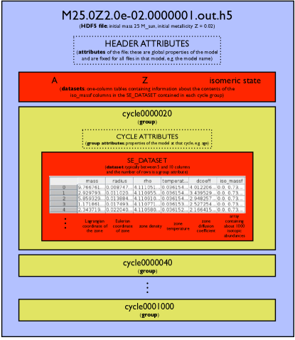
Figure 4: Schematic of SE data format for one-dimensional time-dependent stellar evolution and explosion data.

The time-dependent nature of stellar evolution simulation output suggests for this data a particular structure. For each saved time step, or cycle, a number of scalar quantities have to be saved, as well as a number of profile vectors. A number of such cycles are combined into one data file, or packet. The scalar quantities are the cycle attributes, the profile vectors are the data columns, and each packet has a number of header attributes which are repeated in each file and provide global information for the run, such as initial conditions, code version used, units of quantities in the data columns or cycle attributes, etc. This is the SE (Stellar evolution) data format, shown schematically in Fig. 4 and, within NuGrid, is currently implemented using the hdf5 data format.

SE output from MESA is written with NuGrid’s mesa_h5 and then used for the post-processing simulations using NuGrid’s NuPPN codes, which in turn write output again in the SE format. Libraries and modules to write SE from Fortran, C or Python are available. SE data output can be explored via data access, standard plots, visualisations, and standard analysis procedures, using the NuGridPy Python package.

We want to accommodate three types of user:

• Internal users, including for example students, who are less experienced in the analysis of the NuGrid simulation data.

• Users external to the collaboration to whom we would like to provide the option to explore the NuGrid data set to find answers to their specific research questions.

• Expert users who want to carry out NuGrid and/or MESA simulations and analyse the simulation output conveniently in the same location, and possibly share run directories and workflows. These users can share a common development platform that is exactly identical to each participant who remotely accesses the platform and all of its content.

The first two types of users are served by WENDI, while the third requires additional compilers and libraries which are delivered in mesahub.

4.1.1 WENDI

Web-Exploration for NuGrid Data Interactive WENDI provides

• python and bash notebooks, terminal and text editor;

• example notebooks; and

• self-guided graphical user interface (GUI) notebooks (widgetized notebooks).

The WENDI widget notebook NuGridStarExplorer provides GUI access to plotting and exploring the NuGrid data sets, specifically the library of stellar evolution and detailed nucleosynthesis simulations. As an example, the evolution of a low-metallicity, intermediate mass star is shown during the Asymptotic Giant Branch evolution. The Kippenhahn diagram shows the Lagrangian coordinates of recurring He-shell flashes, each of which drives a pulse-driven convective zone. In the pulse-driven convective zone the ${{{\mathrm{}}}{{\mathrm{{}^{22}}}}{\mathrm{Ne}}}(\alpha,n){{{\mathrm{}}}{{\mathrm{{}^{16}}}}{\mathrm{O}}}$ reaction creates neutrons with neutron densities reaching $N_{n}\approx 10^{12}\mathrm{cm^{-3}}$. At these neutron densities $s$-process branchings, such as at ${{\mathrm{}}}{{\mathrm{{}^{95}}}}{\mathrm{Zr}}$, are activated and the neutron-heavy ${{\mathrm{}}}{{\mathrm{{}^{96}}}}{\mathrm{Zr}}$ is produced. Fig. 6 shows the isotopic abundance distribution of s-process elements. Note, how the mass fraction of ${{\mathrm{}}}{{\mathrm{{}^{96}}}}{\mathrm{Zr}}$ exceeds that of ${{\mathrm{}}}{{\mathrm{{}^{94}}}}{\mathrm{Zr}}$ in the shown model at the end of the pulse-driven convective zone. In the ${{\mathrm{}}}{{\mathrm{{}^{13}}}}{\mathrm{C}}$ pocket where the bulk of the s-process exposure takes place ${{{\mathrm{}}}{{\mathrm{{}^{94}}}}{\mathrm{Zr}}}/{{{\mathrm{}}}{{\mathrm{{}^{96}}}}{\mathrm{Zr}}}\approx 600$ because the neutron denisty is low and the branching is closed. In the solar system ${{{\mathrm{}}}{{\mathrm{{}^{94}}}}{\mathrm{Zr}}}/{{{\mathrm{}}}{{\mathrm{{}^{96}}}}{\mathrm{Zr}}}=6.2$. This demonstrates the different neutron density regimes of the $s$ process. Although this example is for low metal content, conditions at solar-like Z are similar. The solar system abundance distribution originates from a mix of low- and intermediate mass stars, involving both the ${{\mathrm{}}}{{\mathrm{{}^{13}}}}{\mathrm{C}}$ and the ${{\mathrm{}}}{{\mathrm{{}^{22}}}}{\mathrm{Ne}}$ neutron source, which each produce isotopic ratios in different proportions (Gallino et al., 1998; Herwig, 2005, 2013).

Figure 5: Self-guided exploration of the NuGrid stellar evolution and yield data base via the graphical user interface NuGridStarExplorer in WENDI. Kippenhahn diagram of a $\mathrm{M}_{ZAMS}=3\mathrm{M}_{\odot}$ stellar model with $Z=0.001$, zoomed in around the core-envelope interface where the He- (dashed, orange line) and H-burning (solid, blue line) shells are located. Grey and blue areas mark convectively unstable regions and regions of energy generation. The isotopic abundance distribution in the thermal pulse ending around model 16880 is shown in Fig. 6.

Figure 6: Mass-averaged isotopic abundance distribution of the pulse-driven convective zone for model 16880 of the $\mathrm{M}_{ZAMS}=3\mathrm{M}_{\odot}$ stellar model with $Z=0.001$ shown in Fig. 5. The abundance distribution shows the stable isotopes for the first- and second-peak $s$-process elements (see text for more details).

While the widget notebooks provide easy and powerful access to the data, customized analysis may require the added control of programming access to the platform. In order to make it easy for users to get started analyzing the NuGrid data we keep adding to a collection of short example analysis tasks, such as abundance profiles at collapse, or C13-pocket analysis. All data and software dependencies of these examples are satisfied on wendihub. Although users can easily clone their own copy of any external repository, the wendi-examples are preloaded in WENDI, and are a convenient starting point for further analysis. Users who create an interesting new example are encouraged to fork the example repository on the terminal command line, add their new example and make a pull request to the original repository. Although executing notebooks is just a matter of clicking the play button, any further interaction for this type of notebook-based analysis requires basic knowledge in Python.

Two additional widget notebooks are presently available in WENDI. The OMEGA self-guided interface provides example applications of the NuGrid Python Chemical Evolution Environment (NuPyCEE, Ritter & Côté, 2016) code One-zone Model for the Evolution of Galaxies (OMEGA), such as models for dwarf galaxies Fornax, Carina and Sculptor. For OMEGA WENDI allows arbitrary, complex programming of analysis through ipython notebooks as well. For example, the top panel of Fig. 7 shows that NuGrid massive star yields overproduce some iron-peak elements like Cr and Ni, but produce a consistent amount of other elements like Ti, V, Cu, and Ga. Further analysis of the yield source as shown in the IMF-weighted yields (bottom panel) reveals that the overestimation of Cr in the galaxy evolution models originates from the $20\mathrm{M}_{\odot}$ model at $Z=0.01$. This analysis tool allows to identify sources of discrepancies between numerical predictions and observations. In this case, further analysis of the underlying stellar evolution model using similar approaches as those demonstrated below for intermediate-mass stars, that will be presented elsewhere in more detail, connects this overproduction of some iron-group elements to the convective merger of an O-Si shell in the stellar evolution model that may not be realistic. This analysis can be performed by anyone on WENDI, and is available there in a notebook as part of the pre-loaded WENDI examples.

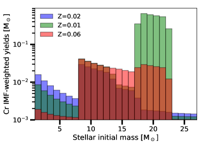
Figure 7: Top: Elemental abundance distribution of the Galactic gas, when the Sun formed, predicted by the chemical evolution code OMEGA using NuGrid yields for low-mass and massive stars and Thielemann et al. (1986) yields for Type-Ia supernovae (SNe Ia). The solar distribution is taken from Lodders et al. (2009). The blue (dashed with triangles), red (dashed with squares), and green (solid with crosses) lines represent the individual contribution of massive stars (winds and core-collapse supernovae), SNe Ia, and low-mass stars, respectively. The orange solid line shows the combined contribution of all sources. Bottom: Cr yields weighted by the initial mass function as a function of stellar mass for different metallicities (different colors) in a $10000\mathrm{M}_{\odot}$ simple stellar population, using NuGrid yields and the SYGMA code. The contribution of SNe Ia is not shown in this panel.

Another widgetized notebook provides an interface for Stellar Yields for Galactic Modelling Applications (SYGMA, Ritter et al., 2017a), which allows to generate simple stellar population models and retrieve chemical yields among other properties in table formats that can be used as building blocks for GCE models or hydrodynamic simulations of galaxy evolution. The SYGMA section of WENDI also contains a folder with notebooks that run the SYGMA code and generate all plots shown in the SYGMA code paper Ritter et al. (2017a). This serves as an example how cyberhubs can be a tool in support of the goal of reproducible science, by providing not only access to data and code, but also to the capability to execute the analysis on the data in a controlled and specified environment.

A technical detail concerns how the widget notebooks are launched. The cyberhubs configuration allows automatic self-start up that hides Python code cells, creating a relatively polished final experience. For this to work, the widget notebooks have to be designated as trusted. Jupyter references a database in a notebook signatures database file which contains instances of the notebooks that are configured to be trusted. In order for a notebook to be trusted, the raw .ipynb notebook file must exactly match the file used to sign said notebook in the database. This system implemented by JupyterHub is rather sensitive to minute changes in the notebook, and does not easily incorporate notebook updates and preserve the trusted state of the previously signed notebook. In order to ensure flexibility of the application hubs with trusted notebooks in their respective singleuser images, even after a notebook has been updated, a bash script is used to trust the notebooks in the state that they exist when staged. This ensures that even if a notebook has changed remotely prior to building a singleuser application hub with a reference to an outdated signatures database, the database will be updated automatically. This script contains a series of paths to the notebooks in the singleuser environment that the user requires to be trusted. When its run, it signs the notebook signatures database file in the singleuser notebook directory.

WENDI is provided by the wendihub docker image that can be found on docker hub (cyberhubs/wendihub) as well as in the astrohubs GitHub repository.

4.1.2 NuGrid / MESA experts

The third of the above cases adds the requirement to install and run multi-core, parallel simulations. The NuGrid collaboration uses the MESA code that uses OpenMP to provide shared memory parallelism scaling to up to $\approx 10$ cores. Like many sophisticated simulation codes MESA relies on a significant number of dependencies. The installation processes has been significantly eased with the MESA-SDK. Still, installation can be a challenge, especially for inexperienced users. The NuGrid code NuPPN for single-, multi-zone and tracer particle processing adopts MPI parallelism and exhibits good strong scaling to $\approx 50$ cores for typical 1D multi-zone problems. Both applications are compiled with the gfortran compiler, and require hdf and se libraries, as well as numerical libraries, such as SuperLU and OpenBLAS. The singleuser application mesahub combines the compilers, libraries and environment variable settings needed to install and run MESA and NuGrid simulation codes, and probably several other codes with the same requirements. The presently latest mesahub docker image (version 0.9.5) runs the NuGrid codes NuPPN/mppnp for parallel multi-zone simulations, and NuPPN/ppn for single-zone simulations, and has been tested for MESA versions 8118, 8845, and 9331. It should be straight-forward to update this application to accommodate newer as well as older MESA versions. The resources of the entire host machine can be accessed by each user through their application docker container. We are currently running cyberhubs on several servers, including one instance on a virtual workstation with 16 cores and 120GB memory which allows several concurrent MESA runs as well as using all 16 cores for NuPPN multi-zone simulations.

In addition, this application includes a wide range of Python packages for data analysis, including NuGrid’s NuGridPy tool box. The application also includes common command-line editors and a complete LaTeX installation that allows manuscript generation, complemented with the browser’s pdf viewer. Jupyter extensions that allow easy generation of interactive slide shows from notebooks for presentations are included. It is therefore possible to perform all steps needed for a research project just inside the mesahub application.

4.2 PPMstar

Another application that we want to highlight is the PPMstarhub which provides analytic access to stellar hydrodynamics simulations (Herwig et al., 2014; Woodward et al., 2015; Jones et al., 2017). The challenges in this case are a combination of very large data sizes and the benefits from using legacy software in a shared environment. This section starts with a historical perspective that provides context for the current development described in this paper.

4.2.1 Data representation strategies for 3D hydrodynamics simulations with PPMstar

Over many years, the team at the University of Minnesota’s Laboratory for Computational Science & Engineering (LCSE) has developed a series of tools to deal with the voluminous data that is generated by collections of large 3-D fluid dynamics simulations. The LCSE was formed in 1995, but the activity began in 1985 as a result of the University of Minnesota’s purchase that year of the largest and most powerful supercomputer then available, the Cray-2. Only 3 of these machines existed in the world at that time. This purchase, coupled with the rarity at the time of academic researchers with simulation codes capable of exploiting this machine, produced an unprecedented opportunity. The university had purchased the machine, but not a data storage system. An early way around that problem for our research team was to take advantage of a holiday sale of disk drives by Control Data, and later the purchase of a tape drive and a small computer to drive it. With this experience, a long tradition of ever greater data compression and development of data analysis and visualization tools began. At the time, there were no data file format standards, nor were there tools, aside from programs one could write oneself, to read such files. The result of this combination of circumstances was that, in the LCSE, we developed our own very powerful tools and techniques to analyze and visualize 3-D simulation data. As the field has grown, other groups have taken it upon themselves to produce, enhance, and maintain such tools for community use, which is a full-time activity that we chose not to engage in. The infrastructure described in this article has provided a framework in which we can embed our LCSE tools, giving them an interface that can be quickly understood and utilized by others through a Web browser. Python is the glue that connects our utilities to the framework and to external users. All this can now make our simulation data available to a community of interested parties around the globe.

Simulations in three dimensions pose special challenges to the understanding of the computational results. LCSE did not embark on 3-D simulation until we heard from a Pixar representative in the mid 1980’s about the invention of volume rendering. Once we saw on a workstation screen the rotating image of the volume rendered water rat that constituted the first demo of the technique, it was obvious to us that this was the solution to the data exploration problem for our fluid dynamics domain. Soon thereafter, we had our first volume rendering program, written by David Porter, running on the Cray-2. This new visualization technique (Porter & Woodward, 1989; Ofelt et al., 1989) prompted the conversion of our 2-D hydrodynamics code to do 3-D simulations. Initially, we tried to save as much of our simulation data as we possibly could, because 3-D fluid dynamics simulation was so new that we thought that we could not possibly predict what representations of the data we might later wish to make. We quickly discovered that we could compress saved data down from 64 to 16 bits per number, saving a factor of 4 in data volume. Even so, the data volume was enormous. Decades of experience with visualizing and analyzing 3-D simulation data (Woodward, 1992a, b, 1993; Tucker & Woodward, 1993) have led us to the approach described below that is connected to the Python-based cyberhubs framework described in this article.

Our simulations fall into fairly simple categories, such as homogeneous turbulence, stellar convection in slab or spherical geometry, or detailed studies of multifluid interface instability growth in slab or spherical geometry. In each category, we do many simulations that all have common features. This has meant that after the first few simulations are completed, we have a very clear idea of what data we want to preserve and what visualizations we want to make of the flows in any new category. We have also developed highly robust nonlinear maps from the real line, or the positive real line, to the interval from 0 to 255. Each such map is determined by an initial functional transformation, such as a logarithm, for example, followed by the standard nonlinear map given by the values of just 2 constant parameters. Such mappings of simulation data to the 256 color levels used in volume rendering can work over all the runs in a single category of simulations without any modification. This is not only tremendously convenient, but it also allows direct and meaningful visual comparisons of data from different runs. It turns out that certain color and opacity maps can work well for a particular simulation variable, such as vorticity magnitude, over an entire category of runs without any modification. These to some degree unexpected findings have profound consequences for data compression.

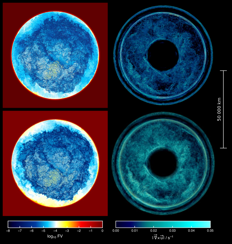
Figure 8: Volume renderings of the volume mixing fraction (left) of hydrogen-rich material pulled into the pulse-driven convective zone in a $2\mathrm{M}_{\odot}$, low metallicity star and of the magnitude of vorticity (right) in this star. In the left column the back hemisphere of the star’s central region is shown, while the vorticity images on the right render a thin slice through the 3D $4\pi$ simulation domain. The volume renderings at the top are made using the full-resolution simulation data, while those at the bottom use the briquette-averaged data (see text for details).

The robustness of nonlinear mappings from the real line to color levels allows us to have our codes dump out only a single byte per grid cell per variable field. This is an enormous savings in data volume. It can only be helpful if one can know before doing the simulation which variables are useful for visual exploration of the simulation results. One can save even more data volume if one knows which views of such variables one wants to preserve. Such images can then be compressed further by standard image file formats. Making this data compression also requires that one know the color and opacity mapping one wishes to use. After a run is completed, these images can now be animated using standard movie making software, such as mencoder, that have replaced our own movie animation software. However, to save only images and not the much more voluminous raw voxel data, one must build the volume renderer into the simulation code. We have done this using the srend software package (Wetherbee et al., 2015). In this way rendering with srend happens right in the code rather than as a separate activity as part of a complex workflow, which has many benefits. The full-resolution voxel data need never be written to disk at all, although, for now, we still write this out just in case. This new capability replaces the previous workflow involving the LCSE HVR volume renderer that required slow and difficult data format conversion, GPUs, and special software libraries to run. srend is written in Fortran, is compiled along with the simulation code, and it has no dependencies upon software libraries. Using either the new srend capability or the previous HVR volume renderer, our strategy is to create default image views of a pre-defined set of variables for all dumps. These image libraries are available through the cyberhub.

Even if we were to continue to save full-resolution voxel data, these data sets are very clumsy to work with due to their sheer size of 45GB per dump depending on how many variables are saved. At the same time, a flexible capability to make any visualization of any variable after the simulation is highly desirable. We accomplish this by performing an additional data compression. This final data compression has evolved from our use of simulation data to validate and develop statistical models of turbulence (Woodward et al., 2006).

Turbulence closure models deal in averages. They tend to be based on comparisons of averages of products and the products of the corresponding averages. To work with such models in the early 2000s, we used averages of our simulation data taken over cubes 32 cells on a side. Our filter represented the behavior of a quantity inside the filter cube by a quadratic form determined by the 10 lowest order moments of the quantity. This filtering technique was derived from our work with the PPB advection scheme (Woodward, 1986; Woodward et al., 2015), which also works with the 10 lowest moments. To be able to construct such filtered representations using a moving filter volume, from our simulations we saved averages of many different variables taken over cubes 4 grid cells on a side. We saved these with 16-bit precision, after first passing them through our robust nonlinear maps.

Our present simulation codes all now work with fundamental data structures consisting of briquettes of 4 grid cells on a side. The problem domain is subdivided into regions, which are rectangular solids, and the regions are subdivided into grid bricks, which are smaller rectangular solids. Each grid brick is a brick of briquettes, augmented all around by a single layer of ghost briquettes from the 26 neighbor bricks.

For the storage required to save just one byte of data from each grid cell in our simulation at any dump time level, we can instead save, with 16-bit precision, 32 variable averages for each grid briquette of 64 cells. 32 variables is so many that we can save several other quantities which require differentiating the simulation data and are useful for model building, in addition to storing variables that we nearly always look at. We include, for example, the magnitude of the vorticity, the divergence of the velocity, and both volume-weighted and mass-weighted averages of the velocity components. The idea is that from the 32 quantities one could derive almost anything one may need when analyzing the data.

Data cubes with the 32 variables representing each of the 216 or 512 regions of a large simulation are saved directly by the code as it runs in separate disk files. In this way the analytic tools have immediate and targeted access to any desired region. In practice, it has been somewhat a surprise how useful the briquette-averaged data actually is. While a fine grid is needed in order to advance the solution in time with high accuracy, this same fine grid is not needed to represent the solution. Volume-rendering from full-resolution images of the mixing fraction and the vorticity are compared with renderings based on the briquette-averaged lower-resolution data sets in Fig. 8. The full-resolution data consists of a single-byte voxel value at each cell of the uniform Cartesian grid to represent each variable we wish to volume render. For the mixing fraction full-resolution means double resolution, i.e. in this case $3072^{3}$ voxels, due to the sub-grid resolving power of the higher-order PPB advection scheme (see appendix of Woodward et al., 2015). The high-resolution rendering of the vorticity and other quantities is based on the grid-resolution data. The lower-resolution renderings of both mixing fraction and vorticity are based on data cubes with four times fewer grid points along each axis. The $384^{3}$ data cubes contain averages of $4\times 4\times 4$-cell briquettes, which for the mixing fraction represent $8\times 8\times 8$ significant data values. The images shown on the top row of Fig. 8 use the full-resolution data, and of course give the best representation. The most important role of renderings and 3D visualisations is to allow a qualitative assessment of the flow, that will ultimately guide quantitative model building. Even renderings based on the 64-times less voluminous briquette-averaged data shown on the bottom row still expose most of the key features of the flow.

Fig. 8 shows the far hemisphere of the He-shell flash convection or pulse-driven convective zone (similar to those shown in Fig. 5 and Fig. 6, see §4.1) in a low-metallicity AGB star. The inner core, including the He shell and a stable layer above that contains H-rich, unprocessed envelope material, is included in the simulation volume. The gas is confined by gravity and also by a reflecting boundary sphere at a radius of $33.5\;\mathrm{Mm}$. The star is shown in the midst of a global oscillation of shell hydrogen ingestion (GOSH, Herwig et al., 2014). H-rich gas is entrained into the pulse-driven convective zone from just above the top of the convection zone, at a radius of about $28\;\mathrm{Mm}$. Waves of combustion involving this mixed-in H and the ${{\mathrm{}}}{{\mathrm{{}^{12}}}}{\mathrm{C}}$ are propagating around the outer portion of the pulse-driven convective zone. The convection zone has been formed by the helium shell flash, with helium burning located at the bottom of the convection zone, around a radius of $13\;\mathrm{Mm}$. The combustion of entrained gas at radii around $17\;\mathrm{Mm}$ drives strong local updrafts, which greatly enhance convective boundary mixing as the combustion waves propagate. This is of course best seen in a movie animation.

In Fig. 8, two counter-propagating wave fronts have recently collided in the region of the lower-left, and a clearly visible puff of entrained gas has been forced downward there, helping to form what will soon become a shell of H-enriched gas floating near the top of the convection zone. In the images at the left the gas of the star’s carbon-oxygen core as well as the helium-and-carbon mixture of the convection zone are rendered as transparent. The color map represents only the H-rich gas component, that initially is confined to the stable layers above the convective boundary. At the point of the simulation shown, some amount of the H-rich fluid has been entrained into the pulse-driven convective zone. From the assumed viewing perspective one sees the lowest H-concentrations first. Where these, rendered dark blue, are sufficiently low, one sees through them into the more highly enriched gas. At this stage, the lower surface of the newly formed shell of H-enriched gas is fairly easily deformed as rising plumes of hotter, more buoyant gas tend to force it aside as they decelerate and ultimately reverse their upward flow. Ridges of dark blue in these images show the lanes that separate neighboring upwellings. These ridges of H-enriched gas are descending, pulling the gas from above the convection zone deeper into the hot region below, where the hydrogen will burn and drive new waves of combustion. All of these key features are clearly discernible in the low-resolution renderings shown in the bottom row of Fig. 8.

Volume renderings of the vorticity magnitude (right column, Fig. 8) reveal a thin, highly turbulent region at the front of the descending puff of entrained gas at the lower left. A typical, unstable shear layer induced by boundary-layer separation (Woodward et al., 2015) can be seen in the upper right quadrant. These features have been identified as an important component of the 3D entrainment mechanism at boundaries that are Kelvin-Helmholtz stable according to the 1D radial stratification. The images based on the briquette-averaged data gives a fuzzy, slightly out-of-focus impression. But they still clearly reveal these key features of the flow, and, when such images are animated, their dynamics.

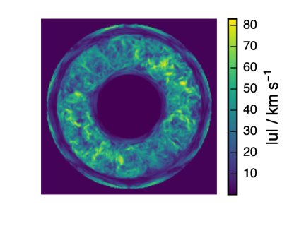
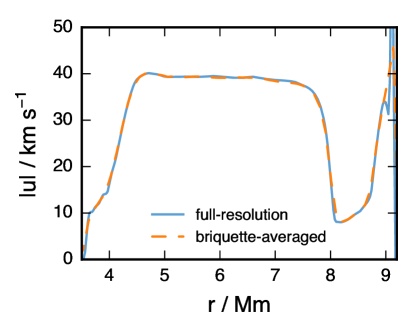
Figure 9: A center-plane slice showing the convective speed from the $768^{3}$-grid O-shell convection simulation D1 presented by Jones et al. (2017), based on briquette-averaged 3D data (top panel), as well as spherically averaged profiles based on full-resolution data and on briquette-averaged data.

Another more quantitative example of how the briquette-averaged data can be used is shown in Fig. 9. Even at a moderately-sized grid of $768^{3}$ the down-sampled data provides a good initial impression of the overall structure of the flow at a computational- and data-related cost that can be easily accommodated in the analysis scenario of the PPMstarhub. For the overall speed profile the low- and high-resolution data representations can hardly be discerned. Even when zooming in to the upper convective boundary the low resolution data provides meaningful exploratory information.

4.2.2 The PPMstar application hub

We have used the cyberhubs technology to build the PPMstarhub application which is addressing several issues. The PPMstar simulations of stellar convection are performed on the Blue Waters computing system at the NCSA center on as many as 400,000 cores. The resulting data sets are in their own way unique, similar to astronomical surveys. Although our team is exploiting them for their primary scientific purpose, there are potentially a number of additional questions that these data sets could answer. Sharing the raw data by just making it available for download is impractical due to the size of the data, as well as the specialized analytic tools that are needed to access and explore the data. cyberhubs allows us to expose to interested users these simulation data sets together with our specialized software stack for analysis.

Over the years, a full range of tools have been developed at the LCSE that exploit the briquette data sets, both for visualization as well as for further analysis that would be involved, for example, in model building. As mentioned above, such models could be turbulence models, or mixing models, to ultimately be deployed in 1D stellar evolution models. These tools are now available along with access to several of our published data sets to interested users through PPMstarHub.

In addition, we have developed additional new Python-based analytic tools that work with the briquette data as well as with single and multiple radial profile data. These, along with collections of example notebooks are available on the PPMstar GitHub repository. Specifically, the examples include notebooks that contain the analysis of all plots shown in our recent study on stellar hydrodynamics of O-shell convection in massive stars (Jones et al., 2017), as well as the notebooks of our project of simulations of low-Z AGB H-ingestion into a thermal-pulse He-shell flash (Woodward et al., in prep). All of these example notebooks are staged on our PPMstarHub server where the necessary data sets are staged as well, so that interested users can follow our data analysis. This is an example of how cyberhubs can play an essential role in making scientific analysis of raw simulation or observational data more transparent and accessible, and the process of data analysis reproducible.

4.3 How to add new applications

The previous sections have described two use cases that have guided the requirements for cyberhubs. Adopting cyberhubs for a different application would start either with the corehub application, or with one of the already existing applications. One would modify the requirements files that specify the Python and Linux software stack, and, following the examples provided, add any custom software and tools required. For example, we have built a basic cyberhubs application image for machine learning (mlhub) and intend to evolve this into a StarNet application for users and developers. StarNet is an application of deep neural networks for the analysis of stellar spectra and especially abundance determination (Fabbro et al., 2017). If one builds a StarNet hub on top of WENDI hub users could perform combined analysis of stellar abundance determination and interpretation of these abundances using, for example, the NuPyCEE tools.

We have also created targeted application for teaching specific courses, such as the second-year computational physics and math course at the University of Victoria, that we are currently teaching with 90 students on the mp248 application that can be optionally launched on the server that also offers the WENDI application.

5 Conclusions

Leveraging dockers, jupyterhub, jupyterlab and jupyter notebook, we designed, implemented and deployed the cyberhubs system. It provides collaborations and research groups with a common collaboration platform in which data, analytic tools, processing capacity as well as different levels of user interactions (Python or bash notebooks, terminals, GUI/widget notebooks). cyberhubs adopts a simple, flexible and effective access and authorization model.

The system is easy to deploy, to customize, and is already in production. By pulling a docker image, cloning a GitHub repository and specifying a few environment variables, administrators can launch VREs for their users. Existing core or more advanced application hub images can be customized to suit specialized needs. In addition to the basic corehub, our specialized hubs are in production and used for collaborations such as NuGrid and PPMstar, as well as in the class room teaching classes with dozens of students.

5.1 Limitations and future development

As with any multiuser platform, the cyberhubs require designated personnel to administrate and maintain, though the deployment of our hubs is straight-forward. The fact that we are dealing with leading edge technologies makes the system susceptible to major changes at any time. We have protected cyberhubs to some degree by enforcing version-locking of each included Python and Linux software package. Although we have frozen the pip and apt requirements by specifying for each component the version to be used at build time to avoid package incompatibility issues, security updates of any package may require the users to update the system. Another limitation of the system is that it does not scale with the number of users, and does not offer resource allocation or scheduling capabilities. As the number of users increases, a cyberhub may run out of resources and larger servers may become necessary. Therefore, we are exploring Docker Swarm and Kubernetes to scale the resources and schedule containers into distributed resources. Volume selection is also an important feature that we plan to add. Depending on the credentials of a user, we are interested in ensuring that the user has access to special/private volumes. We also plan to add letsencrypt capability to our hubs so that administrators are freed from dealing with SSLs directly.

We invite those who are creating new application hub images to share these through adding the build files to the astrohhubs GitHub repository and to submit such images to be pushed to the cyberhubs Docker Hub organisation cyberhubs.

References

- Eggenberger et al. (2008) Eggenberger, P., Meynet, G., Maeder, A., et al. 2008, Ap&SS, 316, 43
- Fabbro et al. (2017) Fabbro, S., Venn, K., O’Briain, T., et al. 2017, eprint arXiv:1709.09182, 1709.09182
- Gallino et al. (1998) Gallino, R., Arlandini, C., Busso, M., et al. 1998, ApJ, 497, 388
- Herwig (2005) Herwig, F. 2005, ARAA, 43, 435
- Herwig (2013) —. 2013, in link.springer.com (Dordrecht: Springer Netherlands), 397–445
- Herwig et al. (2014) Herwig, F., Woodward, P. R., Lin, P.-H., Knox, M., & Fryer, C. 2014, ApJ, 792, L3
- Jones et al. (2017) Jones, S., Andrássy, R., Sandalski, S., et al. 2017, MNRAS, 465, 2991
- Jones et al. (2014) Jones, S., Herwig, F., Siemens, L., et al. 2014, poster contribution at Nuclei in the Cosmos NIC XIII conference, available at http://www.nugridstars.org/publications/conference-contributions/nuclei-in-the-cosmos-xiii/NIC_CADC_poster_best.pdf
- Lodders et al. (2009) Lodders, K., Palme, H., & Gail, H. P. 2009, in Solar System (Berlin, Heidelberg: Springer Berlin Heidelberg), 712–770
- Ofelt et al. (1989) Ofelt, D., Porter, D., Varghese, T., et al. 1989, PPM Graphics Tools, Tech. rep., Minnesota Supercomputer Institute
- Paxton et al. (2010) Paxton, B., Bildsten, L., Dotter, A., et al. 2010, ApJS, 192, 3
- Paxton et al. (2013) Paxton, B., Cantiello, M., Arras, P., et al. 2013, ASTROPHYS J SUPPL S, 208, 4
- Paxton et al. (2015) Paxton, B., Marchant, P., Schwab, J., et al. 2015, ASTROPHYS J SUPPL S, 220, 15
- Pignatari & Herwig (2012) Pignatari, M., & Herwig, F. 2012, Nuclear Physics News, 22, 18
- Pignatari et al. (2016) Pignatari, M., Herwig, F., Hirschi, R., et al. 2016, ASTROPHYS J SUPPL S, 225, 24
- Porter & Woodward (1989) Porter, D. H., & Woodward, P. R. 1989, in ACM SIGGRAPH Video Review, Vol. 44, Volume Visualization State of the Art, ed. L. Herr, 10-minute video segment: Simulations of Compressible Convection with PPM
- Ritter & Côté (2016) Ritter, C., & Côté, B. 2016, NuPyCEE: NuGrid Python Chemical Evolution Environment, Astrophysics Source Code Library, ascl:1610.015
- Ritter et al. (2017a) Ritter, C., Côté, B., Herwig, F., Navarro, J. F., & Fryer, C. 2017a, ApJS submitted, 1711.09172v1
- Ritter et al. (2017b) Ritter, C., Herwig, F., Jones, S., et al. 2017b, MNRAS, submitted, arxiv:1709.08677
- Thielemann et al. (1986) Thielemann, F.-K., Nomoto, K., & Yokoi, K. 1986, A&A, 158, 17
- Tucker & Woodward (1993) Tucker, L., & Woodward, P. R. 1993, System Software and Tools for High Performance Computing Environments (SIAM), 109–113, Paul Messina and Thomas Sterling, eds.
- Wetherbee et al. (2015) Wetherbee, T., Jones, E., Knox, M., Sandalski, S., & Woodward, P. 2015, in Proceedings of the 2015 XSEDE Conference: Scientific Advancements Enabled by Enhanced Cyberinfrastructure (ACM), Article No. 35. https://dl.acm.org/citation.cfm?doid=2792745.2792780
- Woodward (1986) Woodward, P. R. 1986, in Astrophysical Radiation Hydrodynamics, ed. K.-H. Winkler & M. L. Norman, Reidel, 245–326, online at http://www.lcse.umn.edu/PPMlogo
- Woodward (1992a) Woodward, P. R. 1992a, Segment of “Art of Science” program broadcast nationally, PBS, Scientific American Frontiers, produced at Showcase ’92 exhibit at SIGGRAPH
- Woodward (1992b) Woodward, P. R. 1992b, in Proc. Supercomputing Japan, scientific Visualization of Complex Fluid Flow, also available as Minnesota Supercomputer Institute Research Report UMSI 92/233
- Woodward (1993) Woodward, P. R. 1993, in IEEE Computer, Vol. 26
- Woodward et al. (2015) Woodward, P. R., Herwig, F., & Lin, P.-H. 2015, ApJ, 798, 49
- Woodward et al. (2006) Woodward, P. R., Porter, D. H., Anderson, S., Fuchs, T., & Herwig, F. 2006, Journal of Physics Conference Series, 46, 370