Electron Physics in 3D Two-Fluid Ten-Moment Modeling of Ganymede’s Magnetosphere

Abstract

We studied the role of electron physics in 3D two-fluid 10-moment simulation of the Ganymede’s magnetosphere. The model captures non-ideal physics like the Hall effect, the electron inertia, and anisotropic, non-gyrotropic pressure effects. A series of analyses were carried out: 1) The resulting magnetic field topology and electron and ion convection patterns were investigated. The magnetic fields were shown to agree reasonably well with in-situ measurements by the Galileo satellite. 2) The physics of collisionless magnetic reconnection were carefully examined in terms of the current sheet formation and decomposition of generalized Ohm’s law. The importance of pressure anisotropy and non-gyrotropy in supporting the reconnection electric field is confirmed. 3) We compared surface “brightness” morphology, represented by surface electron and ion pressure contours, with oxygen emission observed by the Hubble Space Telescope (HST). The correlation between the observed emission morphology and spatial variability in electron/ion pressure was demonstrated. Potential extension to multi-ion species in the context of Ganymede and other magnetospheric systems is also discussed.

JGR-Space Physics

Space Science Center, University of New Hampshire, Durham, NH 03824, USA Princeton Center for Heliophysics, Princeton Plasma Physics Laboratory, Princeton University, Princeton, NJ 08544, USA Department of Astrophysical Sciences, Princeton University, Princeton, NJ 08544, USA

L. Wangliang.wang@unh.edu

Non-gyrotropic electron pressure tensor effects are important in Ganymede’s magnetic reconnection

Electrons and ions form highly asymmetric and distinct drift patterns in the magnetosphere

Some key features of the observed oxygen emission morphologies are reproduced by the model

1 Introduction

Ganymede, a moon of Jupiter, is not only the largest satellite in the solar system, but also the only satellite that possesses an internal dynamo to generate an intrinsic dipole magnetic field (Gurnett et al., 1996; Kivelson et al., 1996, 1997, 2002). This dipole field interacts with the corotating Jovian plasma and magnetic field, much like the Earth’s dipole interacts with the solar wind in the southward $B_{z}$ situation, to form Ganymede’s own magnetosphere embedded in the enormous magnetosphere of Jupiter. The “incident” Jovian plasma flow is sub-magnetosonic, thus no bow shock is formed around the moon. Instead, a pair of tube-like structures, called Alfvén wings, are induced at the moon, within which the incident plasmas are greatly slowed down (Kivelson et al., 1997).

Ganymede’s magnetosphere is relatively small in terms of the moon’s own size and kinetic scales like particle inertia lengths and gyroradii. This makes it an ideal numerical laboratory for high-resolution investigation of various topics in magnetospheric physics. Previously, the Ganymede’s magnetosphere has been modeled using various models. Kopp and Ip performed single-fluid MHD simulations to reveal the global structure of Ganymede’s field line topology, current system, and convection pattern under different upstream Jovian conditions (Kopp and Ip, 2002; Ip and Kopp, 2002). A series of MHD studies by Jia et al. focused on the details of magnetic reconnection like the formation of Flux Transfer Event (FTE) and discussed its unsteady nature (Jia et al., 2008, 2009, 2010). They also compared different inner boundary conditions at the moon’s surface, and were able to achieve good agreement with in-situ plasma and field measurement when they treated the inner boundary as a plasma sink with finite conductance. Duling et al. (2014) developed a set of rigorous boundary conditions for their MHD simulations, including different conditions for the poloidal and toroidal components of the magnetic field. Their simulations further uncovered the presence of a salty conductive ocean beneath Ganymede’s surface. Paty et al. used multi-ion MHD model to study how different ion species are supplied at the ionosphere and convected and energized in the magnetosphere (Paty and Winglee, 2004, 2006; Paty et al., 2008). They further developed a brightness model to understand the morphology of the Ganymede’s auroral oval (Payan et al., 2015). Later, Dorelli et al. (2015) showed that introduction of Hall effect in an MHD model produced significant asymmetry in plasma flow paths and modified the local field line topology. More recently, Fatemi et al. (2016) used a hybrid model (ions as discrete particles and electrons as massless fluid) to calculate Jovian ion fluxes precipitating on the surface of Ganymede and their correlation to Ganymede’s surface brightness .

A less explored topic is the role of electron kinetic effects. Numerous theoretical analyses, local fully kinetic Particle-In-Cell (PIC) simulations and in-situ observations have confirmed the importance of electron kinetic effects in collisionless magnetic reconnection (Vasyliunas, 1975; Cai and Lee, 1997; Kuznetsova et al., 1998, 2001; Birn et al., 2001; Wang et al., 2000; Ma and Bhattacharjee, 1998; Øieroset et al., 2001). In highly collisionless space plasmas, collisional resistivity is negligible, thus reconnection electric field at the X-line, an important indicator of how fast reconnection is taking place, has to be supported by collisionless effects like the divergence of non-gyrotropic electron pressure tensor (Vasyliunas, 1975; Cai and Lee, 1997; Kuznetsova et al., 1998, 2001; Birn et al., 2001; Øieroset et al., 2001). Since magnetic reconnection is one of the major mechanisms of fast energy conversion and release, its rate can significantly affect the overall structure and evolution of the magnetosphere. How to accurately and efficiently incorporate necessary electron kinetic effects has been a long-standing issue in global modeling of various magnetospheric systems, given the fact that full-domain fully kinetic simulations are much too expensive with contemporary computing power.

One notable attempt to address this issue is the MHD-EPIC approach suggested by Daldorff et al. (2014), which solves MHD or Hall MHD equations in the majority of the domain, but treats plasma as discrete particles (using the implicit PIC method) in prescribed regions where kinetic effects are potentially important. This model has been successfully applied to the Ganymede’s magnetosphere, and demonstrated significant differences compared with standalone Hall MHD results [Tóth et al., 2016]. The MHD-EPIC model has been successfully applied to the Ganymede’s magnetosphere (Tóth et al., 2016). The overall structure of the magnetosphere was similar to that from Hall MHD solution, indicating that kinetic effects do not significantly change the global configuration. But the MHD-EPIC solutions were generally more dynamic than the Hall MHD solutions, producing substantially more and larger FTEs. The MHD-EPIC results also agreed better with Galileo observations in terms of time series and fluctuation spectrum of magnetic field. Beyond the analyses performed by Tóth et al. (2016), the MHD-EPIC model can also be used to study particle acceleration, wave-particle interaction, etc., due to the fully kinetic nature of its PIC component.. However, Tóth et al. (2016) focused more on the general validation of the model and on FTE formation, and did not include dedicated discussion on the roles of electron physics. Their PIC region grid did not fully resolve electron inertia length ($\Delta_{\mathrm{minimum}}\approx 0.8d_{e,\mathrm{Jovian}}$), either, thus the electron effects might have not been accurately modeled. In addition, kinetic dynamics are handled in a few localized box regions to minimize the cost of fully kinetic calculation, but the magnetospheric convection and field-aligned current system are often of global scale, which might also require kinetic treatment.

In this paper, we suggest an alternative approach to incorporate electron (in addition to ion) kinetic effects using higher-order moment multi-fluid models. This model evolves moment equations of each species in the plasma, including both electrons and ions [Hakim et al., 2006; Hakim, 2008; Wang et al., 2015]. Particularly, we focus on the 10-moment sub-model which evolves full pressure tensors, without the isotropic or gyrotropic assumptions. These models solve a hierarchy of velocity-space moment equations truncated at a given order. Depending on the number of moment equations retained, we obtain different “sub-models”(Hakim et al., 2006; Hakim, 2008; Wang et al., 2015). Particularly, we focus on the 10-moment sub-model which evolves the full pressure tensor, in addition to density and momentum, without any isotropy or gyrotropy assumptions. Totally ten independent moment terms (one density, three momenta, and six independent pressure tensor elements) are evolved for each species in the 10-moment sub-model, hence the name (see Section 2 for more details). This way, the electron and ion densities, momenta, and pressure tensors are both directly evolved in time to account for their separate dynamics. Another consequence is that the generalized Ohm’s law embedded in the species momentum equations then automatically contains non-ideal effects like the Hall effect, electron inertia, and divergence of electron pressure tensor, to support the reconnection electric field.Another consequence is that the same physics which are conventionally put into a generalized Ohm’s law are automatically fully included by means of solving all species’ momentum equation directly, coupled via Maxwell’s equations. In particular, the model contains a Hall term, electron pressure tensor and inertia effects. Due to the fluid nature of the model, its computational cost is more comparable to traditional MHD-based codes.

We will perform two-fluid (electron-ion) 10-moment simulations to study the dynamics of both electron and ion flows and the role of electron physics in collisionless reconnection. Key features of the Ganymede’s magnetosphere, particularly the asymmetry in global flow patterspatterns and formation of the auroral oval, will also be investigated. We will not focus on the ionospheric outflow, though, since a relatively simple inner boundary condition is employed, similar to that of (Dorelli et al., 2015; Tóth et al., 2016). The consequences due to this limitation will also be briefly discussed.

The paper is outlined as follows: The equations of the 10-moment model are introduced in Section 2. Initial setup, boundary conditions, and various parameters for the Ganymede simulations are described in Section 3. The simulation results are presented and discussed in Section 4, followed by a summary of findings and implications for future work in Section 5.

2 The 10-Moment Model Equations

The high-moment multi-fluid model is constructed by taking velocity moments of Vlasov equations of each species, including electron, to obtain a hierarchical set of moment equations. Closure is required at the highest truncated moment. For example, in the 10-moment sub-model that truncates at the 2nd order moment, the pressure tensor, assumptions should be made to approximate the 3rd order moment, the heat-flux tensor, depending on the problems studied. In this manner, the high-moment multi-fluid model can, in principle, incorporate even higher-order of moments and thus give a more complete kinetic representation of the plasma than the traditional two-fluid or single-fluid (MHD) model with scalar pressure. Different from MHD-based models which assume charge neutrality and derive electron dynamics indirectly, the high-moment multi-fluid model treats electrons as an independent species and track its evolution. In addition, support of multiple ion species becomes straightforward since we simply need to integrate more sets of moment equations using the same numerical solver.

In this work, we will use the two-fluid (one electron species and one ion species) 10-moment model to model the Ganymede’s magnetosphere. A total of ten equations are solved for each species:

$$\frac{\partial\left(m_{s}n_{s}\right)}{\partial t}+\frac{\partial\left(m_{s}n_{s}u_{j,s}\right)}{\partial x_{j}} = 0,$$ (1)

$$\frac{\partial\left(m_{s}n_{s}u_{j,s}\right)}{\partial t}+\frac{\partial\mathcal{P}_{ij,s}}{\partial x_{j}} = n_{s}q_{s}\left(E_{i}+\epsilon_{ijk}u_{j,s}B_{k}\right),$$ (2)

$$\frac{\partial\mathcal{P}_{ij,s}}{\partial t}+\frac{\partial\mathcal{Q}_{ijm,s}}{\partial x_{m}} = n_{s}q_{s}u_{[i,s}E_{j]}+\frac{q_{s}}{m_{s}}\epsilon_{[iml}\mathcal{P}_{mj],s}B_{l}.$$ (3)

Here, subscripts $s=e,i$ represent the electron and ion species. They will be neglected hereinafter for convenience. The square brackets in equation (3) around indices $ijm$ represent the minimal sum over permutations of these indices that give completely symmetric tensors. The first, second, and third order moments are defined as $mu_{i}\equiv m\int v_{i}fd\mathbf{v}$, $\mathcal{P}_{ij}\equiv m\int v_{i}v_{j}fd\mathbf{v}$, and $\mathcal{Q}_{ijm}\equiv m\int v_{i}v_{j}v_{m}fd\mathbf{v}$, with $f$ being the phase space distribution function. For completeness, $\mathcal{P}_{ij}$ relates to the commonly used thermal pressure tensor $P_{ij}\equiv\int\left(v_{i}-u_{i}\right)\left(v_{j}-u_{j}\right)fd\mathbf{v}$ by

$$\mathcal{P}_{ij}=P_{ij}+nmu_{i}u_{j}.$$

$\mathcal{Q}_{ijm}$ relates to the conventionally defined heat flux tensor $Q_{ijm}\equiv\int(v_{i}-u_{i})(v_{j}-u_{j})(v_{m}-u_{m})fd\mathbf{v}$ by

$$\mathcal{Q}_{ijm}=Q_{ijm}+u_{[i}\mathcal{P}_{jm]}-2nmu_{i}u_{j}u_{m}.$$

Once closed by an approximation to $Q_{ijk}$, the 10-moment equation system self-consistently evolves the pressure tensor for each species. In this paper, we adopt the following simple 3D closure devised by Wang et al. (2015):

$$\partial_{m}Q_{ijm}\approx v_{t}\left|k\right|\left(P_{ij}-p\delta_{ij}\right).$$ (4)

Here, the scalar wave number $k$ is one over a characteristic length scale over which the dominant local physics takes place, $v_{t}$ is the local thermal speed and $p\equiv\left(P_{xx}+P_{yy}+P_{zz}\right)/3$ is the local scalar pressure. In 2D simulation of anti-parallel reconnection presented by Wang et al. (2015), $k$ was chosen to be a constant, $1/d_{e0}$, by arguing that the dominant physics, magnetic reconnection, takes place on the length scale of upstream electron inertia length, $d_{e0}$. In this paper, we relax this requirement by re-calculating $k_{s}$ as $1/d_{s}$ every time step, where $d_{s}$ is the local inertia length of species $s$ at the time step. This should provide more accurate heat flux approximation as species inertia length in the Ganymede problem can vary greatly in space. More recently, Ng et al. (2017) implemented equation (4) in the Fourier transform space ($k-$space) so that the solution in real space ($x$-space) can be recovered by performing invertan inverse Fourier transform. This Fourier transform approach captures non-local heat flux contribution and gives even better agreement with fully kinetic simulation results. However, this approach requires Fast Fourier transform (FFT), which is usually computationally too expensive for large scale systems, and thus is not employed in our magnetosphere modeling here.

The electromagnetic field is evolved by full Maxwell equations

$$\frac{1}{c^{2}}\frac{\partial\mathbf{E}}{\partial t} = \nabla\times\mathbf{B}-\mu_{0}\mathbf{J},$$ (5)

$$\frac{\partial\mathbf{B}}{\partial t} = -\nabla\times\mathbf{E},$$ (6)

thus electromagnetic waves are fully supported, similar to the PIC and Vlasov models. An important difference from traditional MHD-based models is that, the electric field $\mathbf{E}$ in high-moment multi-fluid model is no longer computed explicitly from a given form of the Ohm’s law (e.g., equation (2) of [Dong et al., 2014] (Vasyliunas, 1975; Birn et al., 2001)), but is evolved in time by the Ampere’s law (5). The generalized Ohm’s law is embedded incan be derived from the equation system to include all orders of kinetic effects retained in the moment equations and can be conceptually recovered by combining the electron and ion momentum equations (2).

By including the electron inertia, the dispersive modes (e.g., the whistler) obey the exact dispersion relation which does not produce the quadratic divergence of the oft-quoted dispersion relation obtained by excluding the electron inertia. Thus the explicit time step is not restricted as the dispersive modes grow, unlike inertia-less Hall MHD. The restriction due to Debye length and plasma frequency can also be avoided by using a locally implicit algorithm described by Hakim et al. (2017). Since the restriction due to sound speed is usually relatively mild, the time step is often restricted by speed of light only. For our studies, this restriction can also be efficiently relaxed by using an artificially reduced speed of light.

The high-moment multi-fluid model has been successfully implemented in the computational plasma physics framework, Gkeyll. Non-uniform “stretched” Cartesian grid is supported. The high-resolution wave propagation scheme, a variant of the finite-volume method, is used to solve the hyperbolic equations. The code has been used for many laboratory and space plasma physics projects. For details on the numerics and benchmark examples, please refer to (Hakim et al., 2006; Hakim, 2008; Wang et al., 2000; Hakim et al., 2017).

3 Numerical Setup

We adopt a Cartesian coordinate system following the Ganymede-centered Cartesian system (GphiO) definition (Kivelson et al., 1997): $+x$ is the inflow direction of the corotating Jupiter plasma, $+y$ points from Ganymede to Jupiter, and $+z$ is along the rotation axis. Ganymede is at the origin, and the domain extends from $-64R_{G}$ to $64R_{G}$ in each direction, where $R_{G}=2634.1{\rm km}$ is the radius of Ganymede. The domain is sufficiently large to avoid unphysical reflection to significantly affect physics near the Ganymede during the simulation. A stretched Cartesian $592\times 576\times 576$ grid is employed, with high resolution $\Delta_{\mathrm{minimum}}\approx R_{G}/51$ in the box $\left[-2.5R_{G},2.5R_{G}\right]^{3}$. The grid size is then smoothly ramped up to $1R_{G}$ at $\left|x,y,z\right|=15R_{G}$ and is kept constant further out. We follow the convention in (McGrath et al., 2013) to call the $x<0$ side the upstream or (orbital) trailing side, the $x>0$ side the downstream or (orbital) leading side. They are similar to the definitions of day and night sides at the Earth’s magnetosphere.

The initial magnetic field configuration is defined by the so-called “mirror dipole” setup (for details, see section 2.3 of (Raeder, 2003) or Text S1 in the Supporting Information. In order to avoid large numerical truncation errors, the strong intrinsic dipole field, $\mathbf{B}_{0}$, is treated as a stationary background and does not contribute to the $\nabla\times\mathbf{B}$ term in the Ampere’s law. Only the fluctuating part of the magnetic field, $\mathbf{B}_{1}$, is evolved and included in the $\nabla\times\mathbf{B}$ term. Such separation of background dipole field and induced perturbation field has been adopted in multiple global simulation codes to improve numerical stability (Tanaka, 1994; Tóth et al., 2008; Janhunen et al., 2012). Initially, the plasma density and pressure are uniform throughout the domain with inflow Jovian values, but the velocity is ramped from inflow velocity down to zero over a spherical shell, $2R_{G}<r<2.5R_{G}$. The inflow Jovian wind parameters, intrinsic dipole strength, and other parameters are summarized in Table 1. According to these parameters, the high resolution region resolves the inflow inertia length, $d_{i,in}=\sqrt{m_{i}/\mu_{0}n_{i,in}\left|e\right|^{2}}\approx 474km\approx 0.18R_{G}$, by about $9.2$ cells, and marginally resolves electron inertia length, $d_{e,in}$, by about $1.83$ cells.

The inflow boundary at $x=-64R_{G}$ is set to fixed Jovian values listed in Table 1. All other outer boundaries are set to float (zero-gradient outflow). The inner boundary conditions at surface of Ganymede are as follows: 1) plasma mass densities and pressures are set to constant inflow values; 2) plasma momenta are radially reflected to achieve zero in/out-flow in the steady state; 3) electric field is set to zero; 4) the fluctuating part of the magnetic field $\mathbf{B}_{1}$ is floated. Note that the inner boundary conditions we adopted are simpler than those used by (Jia et al., 2009) and might not achieve as accurate agreement with details of in-situ measurements. Nevertheless, as we will show, the relatively simple boundary conditions are sufficient to correctly reproduce the overall structure of the magnetosphere that agrees reasonably well with observations.

The simulation was performed on Trillian, a Cray XE6m-200 supercomputer at UNH. A total of about 200,000 core hours were used to simulate about 15 minutes of physical time. This is much higher than the cost of a typical single-fluid MHD simulation using the same grid size and time step size, due to its larger number of equations to solve, but would still be significantly cheaper than a fully kinetic simulation of a similar setup.

Table 1: Parameters used in the Ganymede simulation (adapted from (Kivelson et al., 1997; Jia et al., 2010)). Terms with subscript “in” are inflow Jovian parameters. $\mathbf{B}_{G}$ is the Ganymede’s dipole field strength at equitorial surface of the Ganymede. It determines the Ganymede’s dipole field by $\mathbf{B}_{0}=\left[3\left(\mathbf{r}\cdot\mathbf{B}_{G}\right)\mathbf{r}-\mathbf{B}_{G}r^{2}\right]/r^{5}$. Other parameters include $\gamma=5/3$ and $\mu_{0}=4\pi\times 10^{-7}N/A^{2}$.

Parameter	Value
$\rho_{in}\left[amu/cm^{3}\right]$	56
$\mathbf{v}_{in}\left[km/s\right]$	$\left(140,0,0\right)$
$p_{in}\left[nPa\right]$	3.8
$\mathbf{B}_{in}\left[nT\right]$	$\left(0,-6,-77\right)$
$\mathbf{B}_{G}\left[nT\right]$	$\left(-18,51.8,-716.8\right)$
$c\left[km/s\right]$	6000
$m_{i}/m_{e}$	25
$p_{i}/p_{e}$	5

4 Simulation Results

4.1 Overview of basic results

Before dealing with specific non-MHD physics introduced by the 10-moment model, it is crucial to make sure that this model correctly captures essential characteristics of the Ganymede’s magnetosphere, as well as key features of magnetic reconnection.

4.1.1 Global structure of Alfvén wings

A prominent feature of Ganymede is its persisting Alfvén wing structure. It results from the fact that the relative speed of Jovian plasma inflow is sub-Alfvénic and sub-sonic, thus no bow shock is formed ahead of the moon. Instead, the plasma is slowed down significantly within a pair of tube-like structures, called the Alfvén wings, that extend at an angle to the ambient magnetic field for a long distance. The Alfvén wing structure is clearly formed in our simulation. Figure 1 shows the meridional cuts of the electron and ion flow speeds along $x$ direction. The flow speeds are dramatically decreased from the Jovian value $140\mathrm{km/s}$ to as low as $\sim 10\mathrm{km/s}$ in the Alfvén wings. The dashed lines mark boundaries of the wings indicated by the gradient in color contours as well as the diverted flows and abrupt bending of magnetic field lines. The overall Alfvén wing structure is consistent with previous simulation results using various models (Paty and Winglee, 2004; Dorelli et al., 2015; Tóth et al., 2016). In addition, the figure also shows the reconnection outflow jets along $\pm x$ at the downstream X-line near $x\approx 2.5R_{G}$ magnified in panels (c) and (d). Ions are ejected at a bulk speed $\sim 160{\rm km/s}$, while electrons are ejected at a higher speed, about $400{\rm km/s}$. Compared with values identified in the previous MHD-EPIC study by (Tóth et al., 2016), the maximum ion outflow velocity $u_{x,i}$ is similar, but the maximum electron outflow velocity $u_{x,e}$ is slower by half, likely due to the larger relative electron mass used in our study (we used $m_{e}=m_{i}/25$ instead of $m_{i}/100$).

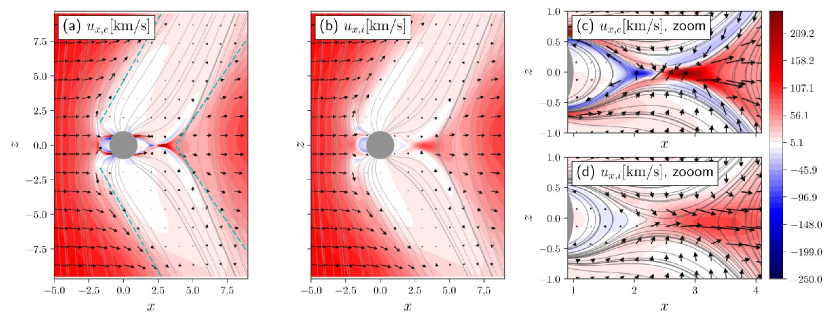
Figure 1: Meridional cuts of electron (panel a and c) and ion (panel b and d) flow speeds along $x$ as colored contours. $u_{x,e}$ and $u_{y,e}$ can reach $\pm 400{\rm km/s}$ and $\pm 160{\rm km/s}$, respectively, but the color map limits are cut and set to be the same for all panels for visualization purpose. Black arrows represent in-plane flows for the two species. Black curves are in-plane magnetic field line. The cyan dashed lines in panel (a) roughly mark the boundaries of the Alfvén wings.

4.1.2 Reconnection current density carrier

The reconnection physics can be further investigated by looking at the reconnection-driven current densities. Figure 2 gives a close look at the out-of-plane electron, ion and total current densities in the meridional plane. Comparing panels (a) and (b), there is a clear separation of thicknesses for the dense electron and ion current sheets, since they scale with electron and ion inertia lengths, respectively. The total current is carried mainly by the lighter electrons consistent with the theoretical expectation. The current sheet extends along the field line separatrices on one end far into the wings, and on the other end down to the Ganymede’s surface. Both $J_{y,e}$ and $J_{y,i}$ are finite upstream of the magnetopause at about $x=-1.8R_{{\rm G}}$, but they cancel each other in this region. No plasmoid generation / FTE formation were observed in this particular simulation. This could be caused by insufficient resolution in electron kinetic scales below which thin current sheets can break into flux tubes, and/or that the uniform $k_{e,i}$ chosen might not best fit the local wave length scales and effectively damped microinstabilities responsible for FTE formation. The size of the magnetosphere is slightly smaller than obtained in previous studies, but is still reasonable. The bottom panels (d) and (e) are cuts of $J_{y,e}$ and $J_{y,i}$ at the downstream side reconnection site. The cut direction is across the current sheet approximately at $x=2.5R_{{\rm G}}$ (and $y=0$) as marked by the vertical dashed lines in panel (a) and (b). The horizontal dashed lines mark the half-maximum locations, which were used to calculate the FWHM (full width half maximum) current sheet thickness. Thus the electron current sheet thickness is around $0.15R_{{\rm G}}\sim 3.8d_{e,{\rm Jovian}}$ and the ion current sheet thickness is about $0.4R_{{\rm G}}\sim 2d_{i,{\rm Jovian}}$ , where $d_{e,{\rm Jovian}}$ and $d_{i,{\rm Jovian}}$ are inertia length based on the upstream Jovian plasma density. This again is consistent with general understanding of current sheet scales in reconnection. This again is consistent with the general kinetic picture that electron and ion current sheet thicknesses are mainly characterized by electron and ion scales, respectively (though the exact scaling laws have not been generally identified) (Wang et al., 2015).

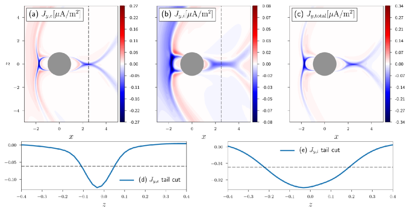
Figure 2: Top, panel (a) to (c): Out-of-plane electron, ion and total current densities in the meridional plane. Bottom, panel (d) and (e): $z$-cuts of electron and ion current densities across the tail current sheets. The cuts are taken at $x=2.5R_{{\rm G}}$ as marked by the dashed lines in panel (a) and (b). The horizontal dashed lines mark $50\%$ maximums of $J_{y,e}$ and $J_{y,i}$.

4.1.3 Comparison with in-situ measurements

Figure 3 shows the simulated and observed magnetic field data along the published G8 flyby trajectory of the Galileo satellite (depicted by the red line in the left panel of Figure 3). The orange solid lines are steadsteady-state modeled values and the blue lines are observed values. The $x$ and $y$ components of the simulated magnetic field agree well with the observed within the majority of the magnetosphere. The simulated $B_{z}$, however, is too flat within the magnetosphere compared to the spatially enhanced values from observation. In addition, the modeled field components do not capture the fluctuations at crossings of the magnetosphere (near 15:50:00 and 16:02:00), either.

We do not cliamclaim to have achieved perfect simulation-observation agreement, noting the fact that the field inside the magnetosphere is dominated by the dipole field, anyway. Previous studies (Paty and Winglee, 2006; Dorelli et al., 2015; Tóth et al., 2016) carried out more sophisticated improvements and achieved more impressivebetter agreement. The discrepancies could result from a few factors: 1) The simplified inner boundary conditions might generate a slightly undersized magnetosphere; Particularly, the series of papers by Jia et al. showed the importance of placing a layer below the moon’s surface, from $1.05R_{\rm{G}}$ down to $0.5R_{\rm{G}}$, in refining the agreement with observations (Jia et al., 2009, 2010). Such a layer is not used in our work (nor in the Hall MHD work by Dorelli et al. (2015) and the MHD-EPIC work by Tóth et al. (2016)), hence the poorer agreement. 2) The simulation parameters do not truly represent the background plasma and field; For example, the ambient $B_{z}$ from Galileo observation is slightly greater in magnitude than what we chose ($-77nT$) to be consistent with prior simulation studies; 3) Dorelli et al. (2015) and Tóth et al. (2016) adjusted the measuring trajectory slightly; [Dorelli et al., 2015] also performed transformation to local boundary norm coordinates (BNC) regarding the magnetopause normal; These adjustments are beyond the scope of this paper thus are not performed here. 4) Previous MHD-EPIC simulation suggested that the fluctuation across the magnetopause might be caused by FTEs, which are not observed in our simulation for multiple potential reasons as we discussed earlier. Nevertheless, consider the relatively simple boundary conditions we employed, the agreement achieved here appears to be reasonably good. The implementation of more realistic inner boundary conditions, as well as the physics of FTEs will be left for future work.

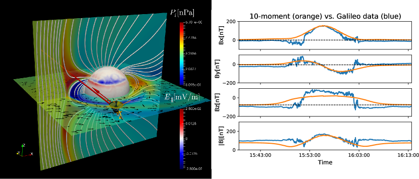
Figure 3: Left panel: The red line and arrow indicate the trajectory and direction of the G8 flyby of the Galileo satellite. The cut views of ion pressure $P_{i}$ and projected magnetic field lines, moon surface electric field $E_{\parallel}$, and ion plasma flow (arrows) are shown to better demonstrate the location of the trajectory. Right panel: Comparison of magnetic field data from our simulation with in-situ measurements by the Galileo magnetometer along the G8 flyby trajectory. The four sub-panels are the three components and magnitude of the observed (blue curves) and simulated (orange curves) magnetic field.

4.2 Pressure tensor effects in collisionless magnetic reconnection

In this section, we focus on the role of electron pressure tensor effect in collisionless reconnection. In a fully kinetic picture, particles are demagnetized near the X-line where the magnetic field is weak, and undergo complex meandering motion within the diffusion region Vasyliunas (1975); Cai and Lee (1997); Bessho et al. (2014, 2016); Zenitani and Nagai (2016). Collectively, these population can drift away from an isotropic and gyrotropic state to form structured distributions in phase space. In the fluid picture, this can lead to pressure anisotropy (unequal diagonal elements) and/or pressure non-gyrotropy (non-vanishing off-diagonal elements) in the pressure tensor. The 10-moment model being a fluid model, motion of discrete paticles and hence the full kinetic distribution function is not tracked. However, our model does allow for the full pressure tensor to evolve according to equation (2), incorporating effects of kinetic origin.

4.2.1 Spatial variation of pressure tensor terms

Figure 4 shows meridional cuts of the pressure tensor elements when the simulation has entered an approximately steady state. The ion scalar pressure, defined by $P_{i}=\frac{1}{3}\left(P_{xx,i}+P_{yy,i}+P_{zz,i}\right)$, is enhanced near the separatrices due to the compression of reconnection driven flows. The spatial pattern of $P_{i}$ is consistent with previous results of (Tóth et al., 2016) (Figure 6). The electron scalar pressure $P_{e}$ is enhanced in more localized regions around the separatrices, and is highest at foot points of the field lines on Ganymede’s surface to form a bright aurora at latitudes $\sim\pm 45^{\circ}$. Non-vanishing off-diagonal elements of the pressure tensor are created along the separatrices where kinetic microphysics is important, while remaining zero elsewhere. The polarities of off-diagonal elements near the X-lines are consistent with previous 2D PIC, Vlasov, and 10-moment simulations (Kuznetsova et al., 2001; Schmitz and Grauer, 2006; Wang et al., 2015) of anti-parallel reconnection when transformed to the corresponding coordinate systems. The magnitudes of these elements are of order $\sim 0.01{\rm nPa}$, considerably smaller than those of diagonal elements (of order $\sim 1{\rm nPa}$). However, the sharp spatial gradient associated with the opposite polarities lead to substantial contribution to the Ohm’s law through the $\nabla\cdot\mathbf{P}_{e}$ term, to be shown later.

Figure 4: Meridional cuts of ion and electron pressure tensor elements at $t=840s$.

4.2.2 Quantification of non-gyrotropy

A quantitative evaluation of the non-gyrotropy is given in Figure 5 showing the measure $\sqrt{Q}$ suggested by (Swisdak, 2016):

$$Q=1-\frac{4I_{2}}{\left(I_{1}-P_{\parallel}\right)\left(I_{1}+3P_{\parallel}\right)}$$ (7)

where $I_{1}=P_{xx}+P_{yy}+P_{zz}$, $I_{2}=P_{xx}P_{yy}+P_{xx}P_{zz}+P_{yy}P_{zz}-P_{xy}^{2}-P_{xz}^{2}-P_{yz}^{2}$, and $P_{\parallel}=\hat{\mathbf{b}}\cdot\mathbf{P}\cdot\hat{\mathbf{b}}$. Here, we have neglected subscripts $e$ that represent electrons. As shown in the meridional view, $\sqrt{Q}$ is intensified near the X-line and along the two ends of open-closed field line separatrices, with maximums just upstream of the X-lines. $\sqrt{Q}$ drops at center of the X-line since the off-diagonal elements drop to zero due to asymmetry. At the time shown, the maxima at the upstream and downstream side X-line are about $0.05$ and $0.03$ respectively, smaller than but still comparable to those found in fully kinetic simulations (Swisdak, 2016; Zenitani and Nagai, 2016). The greater $\sqrt{Q}$ on the upstream side might result from its asymmetric reconnection configuration, consistent with the conclusion in (Swisdak, 2016) that asymmetric reconnection produced a larger $\sqrt{Q}$ than a comparable symmetric reconnection setup. The substantial non-gyrotropy $\sqrt{Q}$ formed in the simulation indicates that the non-gyrotropic pressure effect cannot be neglected.

Figure 5: Meridional and equatorial cuts of the non-gyrotropy measure $\sqrt{Q}$ suggested by Swisdak (2016). Measured at $t=840s$. $\sqrt{Q}$ can vary between 0 for an entirely gyrotropic state and 1 when off-diagonal elements are equal to diagonal elements.

4.2.3 Decomposition of the Ohm’s law

Finally, we examine the contribution of $\nabla\cdot\mathbf{P}_{e}$ in the generalized Ohm’s law. Figure 6 shows 1D line cuts of terms in the Ohm’s law along the inflow direction at the upstream and downstream side reconnection sites. We only show terms in the following $y$ component of the generalized Ohm’s law,

$$E_{y}= (-u_{z,i}B_{x}+u_{x,i}B_{z})+\frac{1}{n_{e}\left|e\right|}(J_{z}B_{x}-J_{x}B_{z})$$ (8)

$$-\frac{1}{n_{e}\left|e\right|}\left(\frac{\partial P_{xy,e}}{\partial x}+\frac{\partial P_{yy,e}}{\partial y}+\frac{\partial P_{yz,e}}{\partial z}\right)$$

$$-\frac{1}{n_{e}\left|e\right|}\left[\frac{\partial\left(\rho_{e}u_{y,e}\right)}{\partial t}+\nabla\cdot\left(\rho\mathbf{u}_{e}u_{y,e}\right)\right].$$

The directly measured $E_{y}$ (blue curve) agrees well with $E_{y,sum}$ (olive curve), the summation of terms on the right hand side of equation (8). For simplicity, the cuts are made across the stagnation point. Overall, the electric field and the decomposed components are highly structured in space. Away from the stagnation point, i.e., from a distance further than electron inertia scale, $E_{y}$ is supported mainly by the convection component $-\mathbf{u}_{e}\times\mathbf{B}$. Near the stagnation point, the convection component drops to near zero and other sources become important.Away from the stagnation point, i.e., from a distance further than the ion inertia length, $E_{y}$ is supported mainly by the convection component $-\mathbf{u}_{i}\times\mathbf{B}$. For the fairly symmetric downstream reconnection, the Hall term (the black curve) is important in the “shoulder” regions on the two sides of the $x$-line where ions are demagnetized but electrons remain largely magnetized. This is consistent with previous understanding of symmetric reconnection (see, e.g., (Wang et al., 2015)). For the upstream crossing, the asymmetry brings in substantially more complexity. For example, the Hall term is smaller on the left side shoulder than on the right side shoulder. Also, the convection term $-\mathbf{u}_{i}\times\mathbf{B}$ passes zero two times, whereas the left passing near $x=-1.75R_{G}$ is near the null point and the right passing is near $x=-1.625R_{G}$ is near the stagnation point. Similar asymmetries occur in local simulations of asymmetric reconnection, too, in qualitatively consistent ways (see, e.g., (Cassak and Shay, 2007)).

Right at the reconnection sites, both the convection term and the Hall term vanish since flow velocities and magnetic field both approach zero, while the $-\nabla\cdot\mathbf{P}_{e}/n_{e}\left|e\right|$ term starts to play an important role in supporting $E_{y}$. For the highly asymmetric upstream side reconnection, the $\partial P_{xy,e}/\partial x$ term is significant, the $\partial P_{yy,e}/\partial y$ that results from the diagonal element gradient is substantially smaller, and the $\partial P_{yz,e}/\partial z$ term is almost negligible. For the fairly symmetric downstream side reconnection, the $\partial P_{xy,e}/\partial x$ term is negligible, and the $\partial P_{yy,e}/\partial y$ and the $\partial P_{yz,e}/\partial z$ terms are significant and comparable in magnitude. The difference in contributing off-diagonal element is due to fact the components are not measured in the same consistent coordinate system regarding the “ambient” magnetic field, which is along $\pm z$ for the upstream side and $\pm x$ for the downstream side. If we rotate the coordinate by $90^{\circ}$ in the $xz$ plane for the upstream side, than we would find consistent results. Nevertheless, it is clear that not only the off-diagonal elements, but also the diagonal elements can contribute to the Ohm’s law in 3D. Particularly, at the downstream side, the scalar gradient term $\partial P_{yy,e}/\partial y$ contribute substantially to $E_{y}$ away from the stagnation point at the time shown. On the other hand, the electron inertia is also important as displayed by the substantial contribution from the flow divergence term $\nabla\cdot\left(\rho_{e}\mathbf{u}_{e}u_{y,e}\right)$ and the time derivative term $\partial\left(\rho\mathbf{u}_{e}\right)/\partial t$.

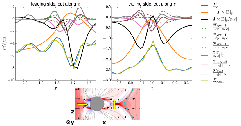
Figure 6: Top row: 1D cuts of terms in the generalized Ohm’s law across upstream (left) and downstreem (right) side current sheets. Only the components out of the reconnection plane, that is, $y$-components are shown. The elements in the $\nabla\cdot\mathbf{P}_{e}$ term are represented by dashed lines. The thick, yellow arrows in the bottom panel indicate directions of the cuts which are along the inflow directions, i.e., along $x$ direction for the upstream side, and along $z$ direction for the downstream side.

4.3 Asymmetric patterns of electrons and ions

Previous MHD-based simulations with single or multiple ion species showed highly asymmetric patterns in surface brightness and bulk flows around the Ganymede (Paty and Winglee, 2004, 2006; Dorelli et al., 2015). However, electron dynamics were derived from assumptions instead of directly evolved in those models since they assume $m_{e}=0$. In the 10-moment model, electrons are incorporated as a separate, independent fluid. We will see that electrons also demonstrate strong spatial variability and contribute significantly to the overall asymmetry due to its negative charge and small, but finite inertia.

4.3.1 Electron vs. ion drift belts

We first look at the equatorial cuts in Figure 7 of electron and ion streamlines over color contours for in-plane speeds. The reconnection electric field and diamagnetic drift at the reconnection sites drives the two species in opposite directions, that is, clockwise for the electrons and anti-clockwise for the ions when viewed from $+z$ direction. The drifts then interact with the incident Jovian inflows to produce very different drift patterns for the two oppositely charged species. Consequently, the locations where the Jovian electron and ion flows enter the “inner magnetosphere” are different. For example, the thickened red lines mark the streamlines that can marginally go around the moon and exit or enter the inner magnetosphere. Also, for both species, the flow patterns are highly structured and sheared. As a result, the streamlines chosen and marked in red and green can be diverted to follow very different paths though they originated from almost the same locations in the Jovian plasma. It also worth noting that, for both species, the flows are accelerated along the X-line to fairly high speeds eventually when they “escape” back to the Jovian plasma in the wake at the Jovian-facing side ($y>0$) for electrons and the other side ($y<0$) for ions. Finally, at the sub-Jovian flank the returning and upstream flows create shears, though we do not observe clear signatures of Kelvin-Helmholtz instability (KHI). Readers are also encouraged to study the 3D image in the Supporting Information (Figure S1) for perspective views of the complex electron and ion flow patterns.

Figure 7: Equatorial cuts of electron (left) and ion (ion) streamlines color coded by the in-plane speed of each species.

4.3.2 Surface brightness

High-speed reconnection outflow jets can propagate along the field line separatrices to hit the Ganymede’s surface and form a bright aurora oval. This process takes place at both upstream and downstream sides of the Ganymede, during which magnetic field-aligned electric field can efficiently energize the plasmas to be observable as enhanced brightness of auroral emissions. Payan et al. developed a sophisticated auroral brightness model in their multi-ion MHD simulation to account for atomic oxygen emission (Payan et al., 2015). Though such brightness model has not been implemented in our 10-moment multi-fluid model, we can get a qualitative picture by using plasma pressures directly as a proxy for brightness.

Figure 8 shows surface morphologies of electron and ion scalar pressure “brightnesses” on the upstream, Jovian-facing, and downstream hemispheres, along with the brightness morphologies due to atomic oxygen emission observed by HST (McGrath et al., 2013). The electron and ion “brightnesses” become fairly stable once the simulation has reached a quasi-steady state, which is consistent with previous observations of repeatable and relatively stable emission patterns (McGrath et al., 2013). The pressures on the upstream hemisphere are enhanced at higher latitudes than on the downstream hemisphere. This is in support of previous hypothesis of acceleration by reconnection electric field since the upstream cusp region is at higher latitude than the downstream cusp. However, the enhancement patters of the two species are very different. For example, on the downstream hemisphere, $p_{e}$ is mostly enhanced near $165^{\circ}{\rm W}$, $30^{\circ}{\rm N/S}$, while $p_{i}$ is mostly enhanced near $30^{\circ}{\rm W}$, $25^{\circ}{\rm N/S}$ (here, following the definition in McGrath et al. (2013), the west/east hemisphere corresponds to the dusk/dawn hemisphere with west longitude $0^{\circ}{\rm W}$ at center the upstream hemisphere, marked by the yellow curves in Figure 8). In comparison, the brightest spots observed by HST are located $90^{\circ}{\rm W}$ on the northern hemisphere, consistent wit the pattern of $p_{i}$ in our simulation, but $90^{\circ}{\rm W}$ on the southern hemisphere, consistent with patterns of $p_{e}$. For the Jovian-facing hemisphere, the enhancement in $p_{e}$ can be barely seen, while $p_{i}$ is clearly enhanced near $330^{\circ}{\rm W}$, $45^{\circ}{\rm N/S}$, very close to the observation. For the upstream hemisphere, the observed high emission regions seem to be consistent with the high $p_{e}$ region in our simulation, but is more stretched. Over all, our simulation captured some key features, e.g., “emissions” at different latitudes on the upstream and downstream hemispheres. The real observed patterns seem to be a complication of modeled electron or ion “brightnesses”. There remain some discrepancies, which are probably due to lack of more realistic inner boundary conditions and that we are modeling only one “average” ion species instead of multiple ones.

Next, we look at the possible role of magnetic-field aligned electric field $E_{\parallel}$ by comparing the electron and ion pressure “brightness” surface maps in Figure 8 with the corresponding maps of $E_{\parallel}$ in Figure 9 (the top row). It is clearly shown that $p_{i}$ tends to be enhanced where $E_{\parallel}$ is positive, while high $p_{e}$ regions tend to correlate with negative $E_{\parallel}$regions. Such tendency is less clear in the southern hemisphere map in the middle column (Jovian-facing) that the negative $E_{\parallel}$ band at latitude $-30^{\circ}$ does not seem to correspond to clear enhancement in $p_{e}$. Nevertheless, the correlation is observedobservable overall. It is worth noting that the $E_{\parallel}$ in our 10-moment simulation is supported by the self-consistently generated pressure tensors divergence and partially by electron inertia effects, instead of numerical or artificially prescribed resistivity. To understand this better, it is also interesting to examine the role of field aligned currents $J_{\parallel,e}$ and $J_{\parallel,i}$ (middle and bottom rows of Figure 9) due to the acceleration by $E_{\parallel}$. The polarities of $J_{\parallel,e}$ and $J_{\parallel,i}$ are closely related to the pressure enhancement patterns. In the northern hemisphere, for example, the magnetic field lines are downward into the moon’s surface, thus positive $J_{\parallel,i}$ corresponds to downward ion flows and thus the enhancement of $P_{i}$ due to pileup of ions at the foot-points. Similarly, negative $J_{\parallel,e}$ corresponds to downward electron flows and hence enhanced $P_{e}$. In the southern hemisphere, the field lines are upward thus the logic applies in the opposite way, i.e., positive $J_{\parallel,e}$ corresponds to $P_{e}$ enhancement.

Finally, Figure 10 shows the latitude-longitude maps of peak brightnesses derived from Figure 8. The peak electron pressure band in the top panel reaches highest latitude $\sim\pm 50^{\circ}$ abruptly near about longitude $300^{\circ}$ and then drops fast. The ion band in the middle panel rises much more gradually and stays at highest latitude over a wider plateau. Both bands, particularly the ion band, approximately agree with in-situ measurements by HST, reproduced in the bottom panel of Figure 10. They are also consistent with the Figure 4 of (Payan et al., 2015) from multi-ion MHD simulations with a more realistic brightness model, particularly the case where the moon is near the center of the Jovian plasma sheet, which is consistent with our simulation setup (flyby G8).

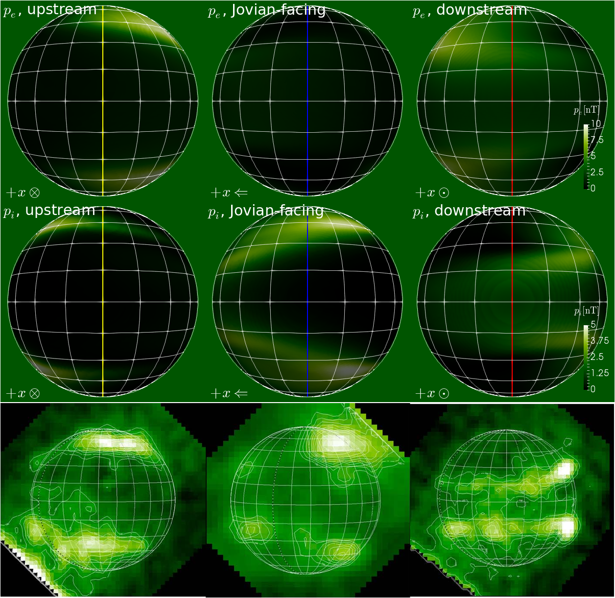
Figure 8: Top and middle rows: Electron (upper row) and ion (lower row) scalar pressures (in units of ${\rm nT}$) on a sphere $263\mathrm{km}$ above the Ganymede surface. The three columns are for the upstream, Jovian-facing and downstream hemispheres. $+z$ points upward in all panels. $+x$ are into the plane, right to left, and out of the plane in the three columns, and are marked at left lower corner of each panel. The red, blue, and yellow curves mark west longitudes $270^{\circ}{\rm W}$, $90^{\circ}{\rm W}$, $0^{\circ}/360^{\circ}{\rm W}$. Third row: Surface brightness from oxygen emission observed by HST. The three images are reproduced from the (c), (b), (a) panels of Figure 2 (upper row) of (McGrath et al., 2013).

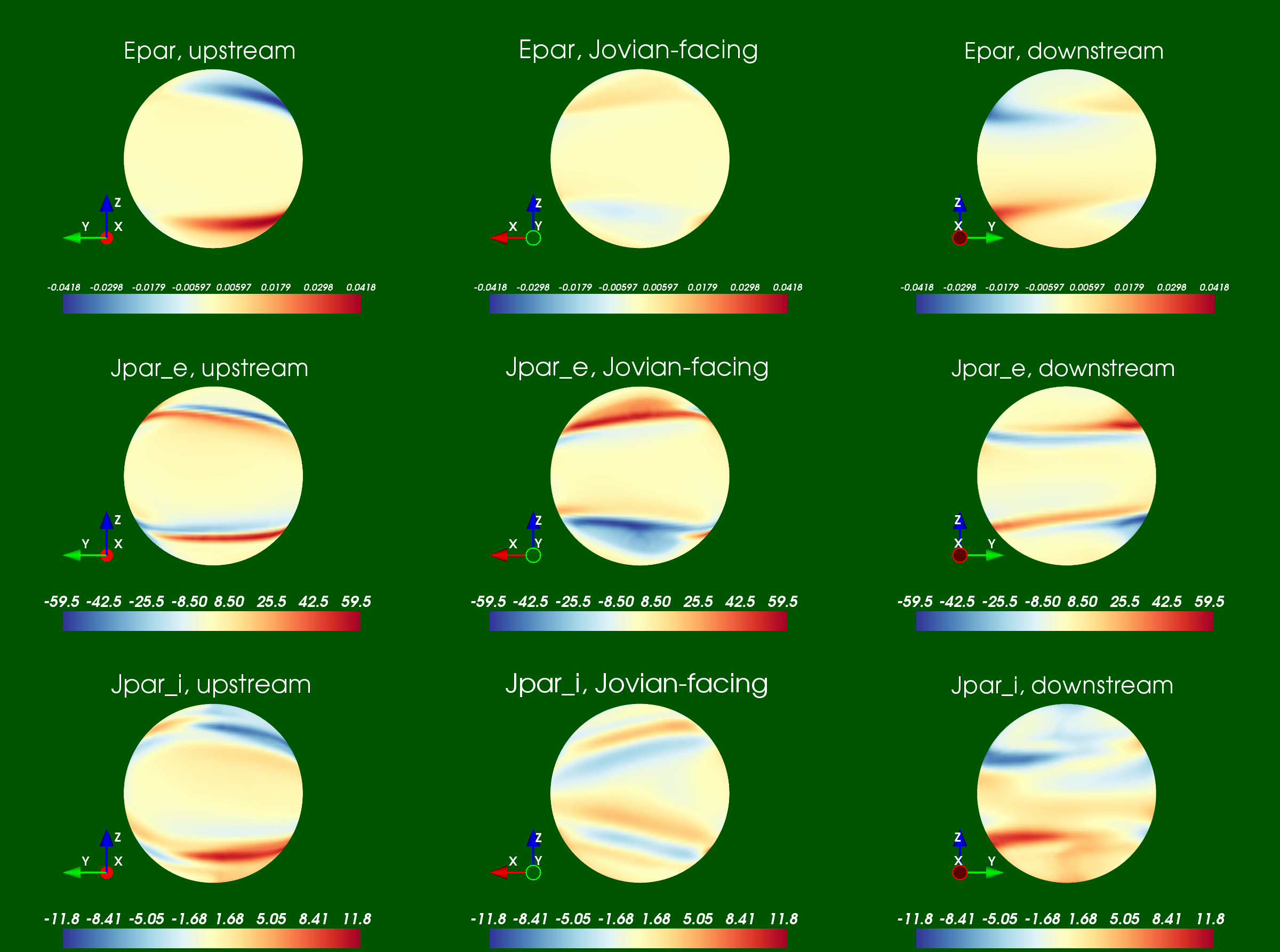
Figure 9: Parallel electric field (top row), electron current (middle row), and ion current (bottom row) on a sphere $263\mathrm{km}$ above the Ganymede surface. The three columns are for the upstream, Jovian-facing and downstream hemispheres, same as Figure 8.

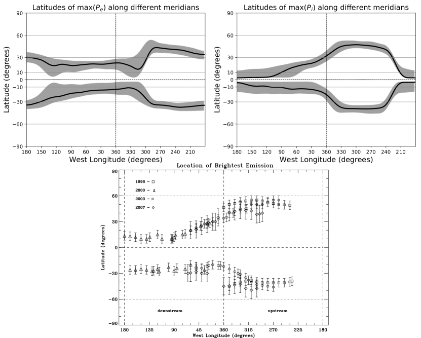
Figure 10: Top panels: Locations of peak pressures, $P_{e}$ and $P_{i}$, on a sphere $263\mathrm{km}$ above the Ganymede’s surface. The solid black curves are the exact locations of maximum values, and the shaded stripes represent regions of values higher than $90\%$ of the maximums. Bottom panel: Locations of peak auroral emission brightness observed by HST in 1998, 2000, 2003, and 2007 (reproduced from Figure 3 of (McGrath et al., 2013)).

5 Discussion and Conclusions

We have successfully modeled Ganymede’s magnetosphere using the 10-moment model. This model provides an efficient way to address deficiencies in modern MHD-based magnetospheric codes, particularly the lack of electron and ion pressure tensor effects. The model correctly captured key features of the Ganymede’s magnetosphere like the Alfvén wing structure and produced magnetic field data that agree reasonably well with in-situ observation. More importantly, the simulation clearly demonstrated, for the first time in the context of realistic 3D magnetosphere, the importance of full electron pressure tensor in collisionless reconnection. In fact, both the diagonal and off-diagonal elements are shown to contribute significantly to the Ohm’s law term $\nabla\cdot\mathbf{P}_{e}$ in 3D. The electron inertia terms were also shown to contribute to the reconnection electric field.

Since the 10-moment model tracks the electron species independently, the effects introduced by electron can be examined straightforwardly. From our simulation, electrons are shown to form asymmetric drift patterns very different from ions, as well as different brightness patterns on the surface of Ganymede. The brightness maps captures some key features observed by the HST/ACS-SBC (McGrath et al., 2013), and could be further refined by using more realistic inner boundary condition and/or more sophisticated brightness model. While the MHD-EPIC model also evolves electron independently and is capable of carrying out similar study in principle, the PIC region employed in (Tóth et al., 2016) did not cover the vicinity of the Ganymede’s surface and such study was not performed.

Compared to the MHD-EPIC model which also aims at incorporating kinetic effects in global modeling, the 10-moment model is computationally less expensive for the same domain size and resolution. The trade-off is that the 10-moment model does not fully retains kinetic effects but truncates at the 2nd order moment. The fluid-representation of the 10-moment model also allows more straightforward coupling with other fluid-based codes like MHD, while the MHD-EPIC approach is generally more difficult to implement due to the vast discrepancy between the MHD model and the PIC model.

One limitation of the 10-moment model is that the inner boundary conditions are more difficultydifficult to set compared to MHD due to the larger number of state quantities. For example, to obtain stable solutions to the Ganymede’s magnetosphere, we set the electric field $\mathbf{E}$ in inner boundary ghost cells to zero, effectively allowing $\mathbf{E}$ to “semi-float”. For a MHD code, boundary condition for $\mathbf{E}$ is not necessary since it is computed from a prescribed form of the Ohm’s law.

This work can be further extended to study multiple topics. For example, our simulation used only one “average” ion species with an average mass and charge. However, in-situ measurements indicated presence of multiple ion species with different masses and temperatures. Multi-fluid MHD simulations by Paty et al. already showed effects of multiple ion species in terms of convection etc, but did not study how the reconnection rate scales with these effects (Paty and Winglee, 2004, 2006; Paty et al., 2008). We plan to incorporate more ion species and study how the global convection and local reconnection dynamics scale with the masses and temperatures of various ion sources. On the other hand, the electron dynamics could be combined with the brightness model suggested by Payan et al. (2015) to give potentially better prediction of aurora emission. Finally, the model may also be applied to other planetary systems, including Mercury and Earth. For example, the 10-moment model can couple with the ionospheric module in the Earth code OpenGGCM to give a more complete picture of magnetospheric physics and possibly more accurate prediction of space weather events.