I Introduction
Millimeter-wave (mmWave) communication is promising to support the vastly growing data traffic for future wireless systems [1 , 2 , 3 ] . In the mmWave band, only several distinctive propagation paths exist, i.e., the line-of-sight path and a few relatively strong reflected paths [4 , 5 ] . Therefore, the directional beamforming with large antenna arrays is necessary to provide sufficiently strong received signal power.
To overcome the hardware limitation on the number of radio frequency (RF) chains with large array size and high carrier frequency, analog beamforming with phased antenna arrays was proposed [6 , 7 , 8 , 9 , 3 ] . A phased array can receive the signal that is projected onto a certain spatial subspace, with a cost of requiring much more pilots than the fully digital arrays to find the rare and precious paths. When users move quickly, it is needed to track the dynamic paths and even more pilots are required. Hence, one fundamental challenge is how to accurately track a large number of dynamic paths from many high-mobility terminals/reflectors using limited pilots, e.g., in V2V/V2I, high-speed railway, and UAV scenarios [10 ] .
The compressed sensing based algorithms (e.g., [11 , 12 , 13 ] ) were proposed for phased arrays, which can reduce pilot overhead and make beam direction acquisition faster. However, these algorithms are designed for static or quasi-static scenarios, and will encounter performance deterioration under high-mobility scenarios. To cope with high-mobility scenarios, the algorithms in [14 , 15 , 16 ] use the prior information to track the dynamic beam directions. However, these solutions do not optimize the tracking scheme with the optimal training beamforming vectors, which leads to poor tracking accuracy.
Since the tracking of a large number of dynamic paths can be decoupled into tracking each path with low pilot overhead, we have proposed a beam tracking algorithm in [17 , 18 ] to optimize both the training beamforming vectors and tracking scheme. However, it assumes known channel coefficients, while both channel coefficient and beam direction might be unknown and time-varying in a real mobile system. In this paper, we further develop a recursive beam and channel tracking (RBCT) algorithm to jointly track the dynamic beam direction and channel coefficient.
In static scenarios, the Cramér-Rao lower bound (CRLB) of beam direction is derived, which is a function of the training beamforming vectors. We also obtain the minimum CRLB by optimizing these training beamforming vectors, and establish three theorems to verify that the RBCT algorithm can converge to the minimum CRLB with high probability. Simulations reveal that the RBCT algorithm can achieve much faster tracking speed, lower tracking error, and lower pilot overhead than several existing algorithms.
We use the following notations: 𝐀 𝐀 \mathbf{A} 𝐚 𝐚 \mathbf{a} a 𝑎 a ‖ 𝐀 ‖ 2 subscript norm 𝐀 2 \left\|\mathbf{A}\right\|_{2} 𝐀 𝐀 \mathbf{A} 𝐀 T superscript 𝐀 T \mathbf{A}^{\text{T}} 𝐀 H superscript 𝐀 H \mathbf{A}^{\text{H}} 𝐀 − 1 superscript 𝐀 1 \mathbf{A}^{-1} 𝐀 𝐀 \mathbf{A} 𝔼 [ ⋅ ] 𝔼 delimited-[] ⋅ \mathbb{E}[\cdot] Re { ⋅ } Re ⋅ \operatorname{Re}\left\{\cdot\right\} Im { ⋅ } Im ⋅ \operatorname{Im}\left\{\cdot\right\} x 𝑥 x log ( x ) 𝑥 \log(x)
II System Model
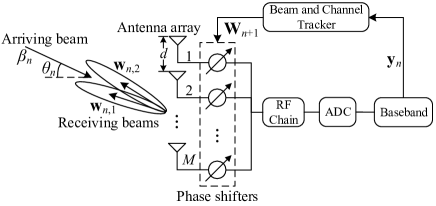
Consider a phased array in Fig. 1 M 𝑀 M omnidirectional antennas are placed on a line, with a distance d 𝑑 d Each antenna is connected through a phase shifter to the same RF chain. In time-slot n 𝑛 n θ n ∈ [ − π 2 , π 2 ] subscript 𝜃 𝑛 𝜋 2 𝜋 2 \theta_{n}\!\in\![-\frac{\pi}{2},\frac{\pi}{2}]
𝐡 n = β n 𝐚 ( x n ) , subscript 𝐡 𝑛 subscript 𝛽 𝑛 𝐚 subscript 𝑥 𝑛 \mathbf{h}_{n}=\beta_{n}\mathbf{a}(x_{n}), (1)
where x n = sin ( θ n ) subscript 𝑥 𝑛 subscript 𝜃 𝑛 x_{n}\!=\!\sin(\theta_{n}) θ n subscript 𝜃 𝑛 \theta_{n} 𝐚 ( x n ) = [ 1 , e j 2 π d λ x n , ⋯ , e j 2 π d λ ( M − 1 ) x n ] H 𝐚 subscript 𝑥 𝑛 superscript 1 superscript 𝑒 𝑗 2 𝜋 𝑑 𝜆 subscript 𝑥 𝑛 ⋯ superscript 𝑒 𝑗 2 𝜋 𝑑 𝜆 𝑀 1 subscript 𝑥 𝑛
H \mathbf{a}(x_{n})\!\!=\!\!\left[1,\!e^{j\frac{2\pi d}{\lambda}x_{n}},\!\cdots,\!e^{j\frac{2\pi d}{\lambda}(M\!-\!1)x_{n}}\right]^{\text{H}} λ 𝜆 \lambda β n = β n re + j β n im subscript 𝛽 𝑛 subscript superscript 𝛽 re 𝑛 𝑗 subscript superscript 𝛽 im 𝑛 \beta_{n}\!=\!\beta^{\text{re}}_{n}\!+\!j\beta^{\text{im}}_{n}
Figure 1: System model.
To track the beam direction x n subscript 𝑥 𝑛 x_{n} β n subscript 𝛽 𝑛 \beta_{n} applied in each time-slot. To receive the i 𝑖 i i = 1 , 2 𝑖 1 2
i=1,2 𝐰 n , i subscript 𝐰 𝑛 𝑖
\mathbf{w}_{n,i} beamforming vector in time-slot n 𝑛 n
𝐰 n , i = 𝐚 ( x n + δ n , i ) M , subscript 𝐰 𝑛 𝑖
𝐚 subscript 𝑥 𝑛 subscript 𝛿 𝑛 𝑖
𝑀 \mathbf{w}_{n,i}=\frac{\mathbf{a}(x_{n}+\delta_{n,i})}{\sqrt{M}},\vspace{-2.5mm} (2)
which is assumed to have the same form as the steering vector. Combining the output signals of the phase shifters yields
y n , i = 𝐰 n , i H 𝐡 n s + z n , i = β n 𝐰 n , i H 𝐚 ( x n ) s + z n , i , subscript 𝑦 𝑛 𝑖
superscript subscript 𝐰 𝑛 𝑖
H subscript 𝐡 𝑛 𝑠 subscript 𝑧 𝑛 𝑖
subscript 𝛽 𝑛 superscript subscript 𝐰 𝑛 𝑖
H 𝐚 subscript 𝑥 𝑛 𝑠 subscript 𝑧 𝑛 𝑖
\displaystyle y_{n,i}=\mathbf{w}_{n,i}^{\text{H}}\mathbf{h}_{n}{s}+{z}_{n,i}=\beta_{n}\mathbf{w}_{n,i}^{\text{H}}\mathbf{a}(x_{n}){s}+{z}_{n,i}, (3)
where s 𝑠 {s} z n , i ∼ 𝒞 𝒩 ( 0 , σ 0 2 ) similar-to subscript 𝑧 𝑛 𝑖
𝒞 𝒩 0 superscript subscript 𝜎 0 2 {z}_{n,i}\!\sim\!\mathcal{CN}(0,\sigma_{0}^{2}) i.i.d. circularly symmetric complex Gaussian random variable. Given 𝝍 n = [ β n re , β n im , x n ] T subscript 𝝍 𝑛 superscript subscript superscript 𝛽 re 𝑛 subscript superscript 𝛽 im 𝑛 subscript 𝑥 𝑛
T \boldsymbol{\psi}_{n}\!=\![\beta^{\text{re}}_{n},\beta^{\text{im}}_{n},x_{n}]^{\text{T}} 𝐖 n = [ 𝐰 n , 1 , 𝐰 n , 2 ] subscript 𝐖 𝑛 subscript 𝐰 𝑛 1
subscript 𝐰 𝑛 2
\mathbf{W}_{n}\!=\!\left[\mathbf{w}_{n,1},\mathbf{w}_{n,2}\right] 𝐲 n = [ y n , 1 , y n , 2 ] T subscript 𝐲 𝑛 superscript subscript 𝑦 𝑛 1
subscript 𝑦 𝑛 2
T \mathbf{y}_{n}\!=\![y_{n,1},y_{n,2}]^{\text{T}}
p ( 𝐲 n | 𝝍 n , 𝐖 n ) = 1 π 2 σ 0 4 e − ‖ 𝐲 n − s β n 𝐖 n H 𝐚 ( x n ) ‖ 2 2 σ 0 2 . 𝑝 conditional subscript 𝐲 𝑛 subscript 𝝍 𝑛 subscript 𝐖 𝑛
1 superscript 𝜋 2 superscript subscript 𝜎 0 4 superscript 𝑒 subscript superscript norm subscript 𝐲 𝑛 𝑠 subscript 𝛽 𝑛 superscript subscript 𝐖 𝑛 H 𝐚 subscript 𝑥 𝑛 2 2 superscript subscript 𝜎 0 2 \displaystyle p(\mathbf{y}_{n}|\boldsymbol{\psi}_{n},\mathbf{W}_{n})=\frac{1}{\pi^{2}\sigma_{0}^{4}}e^{-\frac{\left\|\mathbf{y}_{n}-{s}\beta_{n}\mathbf{W}_{n}^{\text{H}}\mathbf{a}(x_{n})\right\|^{2}_{2}}{\sigma_{0}^{2}}}. (4)
A beam and channel tracker determines the beamforming matrix 𝐖 n subscript 𝐖 𝑛 \mathbf{W}_{n} 𝝍 ^ n = [ β ^ n re , β ^ n im , x ^ n ] T subscript ^ 𝝍 𝑛 superscript subscript superscript ^ 𝛽 re 𝑛 subscript superscript ^ 𝛽 im 𝑛 subscript ^ 𝑥 𝑛
T \hat{\boldsymbol{\psi}}_{n}\!=\![\hat{\beta}^{\text{re}}_{n},\hat{\beta}^{\text{im}}_{n},\hat{x}_{n}]^{\text{T}} β n subscript 𝛽 𝑛 \beta_{n} x n subscript 𝑥 𝑛 x_{n} ξ = ( 𝐖 1 , 𝐖 2 , … , 𝝍 ^ 1 , 𝝍 ^ 2 , … ) 𝜉 subscript 𝐖 1 subscript 𝐖 2 … subscript ^ 𝝍 1 subscript ^ 𝝍 2 … \xi\!=\!(\mathbf{W}_{1},\mathbf{W}_{2},\ldots,\hat{\boldsymbol{\psi}}_{1},\hat{\boldsymbol{\psi}}_{2},\ldots) beam and channel tracking policy . In particular, we consider the set Ξ Ξ \Xi causal beam and channel tracking policies: The estimate 𝝍 ^ n subscript ^ 𝝍 𝑛 \hat{\boldsymbol{\psi}}_{n} n 𝑛 n 𝐖 n + 1 subscript 𝐖 𝑛 1 \mathbf{W}_{n+1} n + 1 𝑛 1 n+1 ( 𝐖 1 , … , 𝐖 n ) subscript 𝐖 1 … subscript 𝐖 𝑛 (\mathbf{W}_{1},\ldots,\mathbf{W}_{n}) ( 𝐲 1 , … , 𝐲 n ) subscript 𝐲 1 … subscript 𝐲 𝑛 (\mathbf{y}_{1},\ldots,\mathbf{y}_{n})
IV Recursive Beam and Channel Tracking
Figure 3: Frame structure.
We propose a two-stage algorithm to approach the minimum CRLB in (III-A
Recursive Beam and Channel Tracking (RBCT):
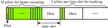
1) Coarse Beam Sweeping: M 𝑀 M 3 m 𝑚 m y ~ m subscript ~ 𝑦 𝑚 \tilde{y}_{m} 𝐰 ~ m = 1 M 𝐚 ( 2 m M − M + 1 M ) , m = 1 , … , M formulae-sequence subscript ~ 𝐰 𝑚 1 𝑀 𝐚 2 𝑚 𝑀 𝑀 1 𝑀 𝑚 1 … 𝑀
\tilde{\mathbf{w}}_{m}\!=\!\frac{1}{\sqrt{M}}\mathbf{a}\left(\frac{2m}{M}-\frac{M+1}{M}\right),m\!=\!1,\ldots,M 𝝍 ^ 0 = [ β ^ 0 re , β ^ 0 im , x ^ 0 ] T subscript ^ 𝝍 0 superscript subscript superscript ^ 𝛽 re 0 subscript superscript ^ 𝛽 im 0 subscript ^ 𝑥 0
T \hat{\boldsymbol{\psi}}_{0}\!=\![\hat{\beta}^{\text{re}}_{0},\hat{\beta}^{\text{im}}_{0},\hat{x}_{0}]^{\text{T}}
x ^ 0 = arg max x ^ ∈ 𝒳 | 𝐚 ( x ^ ) H 𝐖 ~ 𝐲 ~ | , β ^ 0 = [ 𝐖 ~ H 𝐚 ( x ^ 0 ) ] + 𝐲 ~ , formulae-sequence subscript ^ 𝑥 0 ^ 𝑥 𝒳 𝐚 superscript ^ 𝑥 H ~ 𝐖 ~ 𝐲 subscript ^ 𝛽 0 superscript delimited-[] superscript ~ 𝐖 H 𝐚 subscript ^ 𝑥 0 ~ 𝐲 \displaystyle\hat{x}_{0}\!=\!\underset{\hat{x}\in\mathcal{X}}{\arg\max}\left|\mathbf{a}(\hat{x})^{\text{H}}\tilde{\mathbf{W}}\tilde{\mathbf{y}}\right|,\hat{\beta}_{0}\!=\!\left[\tilde{\mathbf{W}}^{\text{H}}\mathbf{a}(\hat{x}_{0})\right]^{+}\!\!\tilde{\mathbf{y}}, (11)
where 𝐲 ~ = [ y ~ 1 , … , y ~ M ] T ~ 𝐲 superscript subscript ~ 𝑦 1 … subscript ~ 𝑦 𝑀
T \tilde{\mathbf{y}}=[\tilde{y}_{1},\ldots,\tilde{y}_{M}]^{\text{T}} 𝐖 ~ = [ 𝐰 ~ 1 , … , 𝐰 ~ M ] ~ 𝐖 subscript ~ 𝐰 1 … subscript ~ 𝐰 𝑀
\tilde{\mathbf{W}}=[\tilde{\mathbf{w}}_{1},\ldots,\tilde{\mathbf{w}}_{M}] 𝒳 = { 1 − M 0 M 0 , 3 − M 0 M 0 , … , M 0 − 1 M 0 } 𝒳 1 subscript 𝑀 0 subscript 𝑀 0 3 subscript 𝑀 0 subscript 𝑀 0 … subscript 𝑀 0 1 subscript 𝑀 0 \mathcal{X}=\left\{\frac{1-M_{0}}{M_{0}},\frac{3-M_{0}}{M_{0}},\ldots,\frac{M_{0}-1}{M_{0}}\right\} M 0 ( M 0 ≥ M ) subscript 𝑀 0 subscript 𝑀 0 𝑀 M_{0}(M_{0}\geq M) 𝒳 𝒳 \mathcal{X} 𝐗 + = Δ ( 𝐗 H 𝐗 ) − 1 𝐗 H superscript 𝐗 Δ superscript superscript 𝐗 H 𝐗 1 superscript 𝐗 H \mathbf{X}^{+}\overset{\Delta}{=}(\mathbf{X}^{\text{H}}\mathbf{X})^{-1}\mathbf{X}^{\text{H}}
2) Beam and Channel Tracking: In time-slot n 𝑛 n 3 𝐰 n , 1 subscript 𝐰 𝑛 1
\mathbf{w}_{n,1} 𝐰 n , 2 subscript 𝐰 𝑛 2
\mathbf{w}_{n,2}
𝐰 n , 1 = 𝐚 ( x ^ n − 1 − δ ∗ ) M , 𝐰 n , 2 = 𝐚 ( x ^ n − 1 + δ ∗ ) M , formulae-sequence subscript 𝐰 𝑛 1
𝐚 subscript ^ 𝑥 𝑛 1 superscript 𝛿 𝑀 subscript 𝐰 𝑛 2
𝐚 subscript ^ 𝑥 𝑛 1 superscript 𝛿 𝑀 \displaystyle\mathbf{w}_{n,1}=\frac{\mathbf{a}(\hat{x}_{n-1}-\delta^{*})}{\sqrt{M}},~{}\mathbf{w}_{n,2}=\frac{\mathbf{a}(\hat{x}_{n-1}+\delta^{*})}{\sqrt{M}}, (12)
and the estimate 𝝍 ^ n = [ β ^ n re , β ^ n im , x ^ n ] T subscript ^ 𝝍 𝑛 superscript subscript superscript ^ 𝛽 re 𝑛 subscript superscript ^ 𝛽 im 𝑛 subscript ^ 𝑥 𝑛
T \hat{\boldsymbol{\psi}}_{n}\!=\![\hat{\beta}^{\text{re}}_{n},\hat{\beta}^{\text{im}}_{n},\hat{x}_{n}]^{\text{T}} 13 𝐠 ^ n = 𝐖 n H 𝐚 ( x ^ n − 1 ) subscript ^ 𝐠 𝑛 superscript subscript 𝐖 𝑛 H 𝐚 subscript ^ 𝑥 𝑛 1 \hat{\mathbf{g}}_{n}\!=\!\mathbf{W}_{n}^{\text{H}}\mathbf{a}(\hat{x}_{n\!-\!1}) 𝐞 ^ n = β ^ n − 1 𝐖 n H 𝐚 ˙ ( x ^ n − 1 ) subscript ^ 𝐞 𝑛 subscript ^ 𝛽 𝑛 1 superscript subscript 𝐖 𝑛 H ˙ 𝐚 subscript ^ 𝑥 𝑛 1 \hat{\mathbf{e}}_{n}\!=\!\hat{\beta}_{n\!-\!1}\mathbf{W}_{n}^{\text{H}}\dot{\mathbf{a}}(\hat{x}_{n\!-\!1}) l n = ‖ 𝐠 ^ n ‖ 2 ‖ 𝐞 ^ n ‖ 2 subscript 𝑙 𝑛 subscript norm subscript ^ 𝐠 𝑛 2 subscript norm subscript ^ 𝐞 𝑛 2 l_{n}=\|\hat{\mathbf{g}}_{n}\|_{2}\|\hat{\mathbf{e}}_{n}\|_{2} c n = 𝐠 ^ n H 𝐞 ^ n subscript 𝑐 𝑛 superscript subscript ^ 𝐠 𝑛 H subscript ^ 𝐞 𝑛 c_{n}=\hat{\mathbf{g}}_{n}^{\text{H}}\hat{\mathbf{e}}_{n}
In Stage 1 , the exhaustive sweeping is used, and the initial estimate 𝝍 ^ 0 subscript ^ 𝝍 0 \hat{\boldsymbol{\psi}}_{0} 11 [13 ] ). This ensures that the initial beam direction x ^ 0 subscript ^ 𝑥 0 \hat{x}_{0}
ℬ ( x 0 ) = Δ ( x 0 − λ M d , x 0 + λ M d ) . ℬ subscript 𝑥 0 Δ subscript 𝑥 0 𝜆 𝑀 𝑑 subscript 𝑥 0 𝜆 𝑀 𝑑 \mathcal{B}\left(x_{0}\right)\overset{\Delta}{=}\Big{(}x_{0}-\frac{\lambda}{Md},x_{0}+\frac{\lambda}{Md}\Big{)}. (14)
In Stage 2 , the recursive tracker is motivated by the following maximization likelihood problem:
max 𝝍 ^ n { max 𝐖 n ∑ i = 1 n 𝔼 [ log p ( 𝐲 i | 𝝍 ^ n , 𝐖 i ) | 𝝍 ^ n , 𝐖 1 , … , 𝐖 i , 𝐲 1 , … , 𝐲 i − 1 ] } , subscript ^ 𝝍 𝑛 subscript 𝐖 𝑛 superscript subscript 𝑖 1 𝑛 𝔼 delimited-[] conditional 𝑝 conditional subscript 𝐲 𝑖 subscript ^ 𝝍 𝑛 subscript 𝐖 𝑖
matrix subscript ^ 𝝍 𝑛 subscript 𝐖 1 … subscript 𝐖 𝑖
subscript 𝐲 1 … subscript 𝐲 𝑖 1
\!\underset{\hat{\boldsymbol{\psi}}_{n}}{\max}\!\left\{\!\underset{\mathbf{W}_{n}}{\max}~{}\!\!\!\sum_{i=1}^{n}\mathbb{E}\bigg{[}\!\log p\!\left(\mathbf{y}_{i}|\hat{\boldsymbol{\psi}}_{n},\!\mathbf{W}_{i}\!\right)\!\!\bigg{|}\begin{matrix}\hat{\boldsymbol{\psi}}_{n},\!\mathbf{W}_{1},\!\ldots,\!\mathbf{W}_{i},\\
\!\mathbf{y}_{1},\!\ldots,\!\mathbf{y}_{i-1}\end{matrix}\bigg{]}\!\right\}\!\!,\!\! (15)
where 𝐖 n = [ 𝐰 n , 1 , 𝐰 n , 2 ] subscript 𝐖 𝑛 subscript 𝐰 𝑛 1
subscript 𝐰 𝑛 2
\mathbf{W}_{n}\!=\!\left[\mathbf{w}_{n,1},\!\mathbf{w}_{n,2}\right] 2 15 outer layer , we use the stochastic Newton’s method to update the estimate 𝝍 ^ n subscript ^ 𝝍 𝑛 \hat{\boldsymbol{\psi}}_{n} [19 ]
𝝍 ^ n = subscript ^ 𝝍 𝑛 absent \displaystyle\!\!\!\!\hat{\boldsymbol{\psi}}_{n}\!=\! 𝝍 ^ n − 1 − a n 𝔼 [ 𝐇 ( 𝝍 ^ n − 1 , 𝐖 n ) ] − 1 ⋅ ∂ log p ( 𝐲 n | 𝝍 ^ n − 1 , 𝐖 n ) ∂ 𝝍 ^ n − 1 subscript ^ 𝝍 𝑛 1 ⋅ subscript 𝑎 𝑛 𝔼 superscript delimited-[] 𝐇 subscript ^ 𝝍 𝑛 1 subscript 𝐖 𝑛 1 𝑝 conditional subscript 𝐲 𝑛 subscript ^ 𝝍 𝑛 1 subscript 𝐖 𝑛
subscript ^ 𝝍 𝑛 1 \displaystyle~{}\hat{\boldsymbol{\psi}}_{n\!-\!1}\!-\!a_{n}\mathbb{E}\!\left[\mathbf{H}(\hat{\boldsymbol{\psi}}_{n\!-\!1},\!\mathbf{W}_{n})\right]^{-1}\!\cdot\!\frac{\partial\log p(\mathbf{y}_{n}|\hat{\boldsymbol{\psi}}_{n\!-\!1},\!\mathbf{W}_{n})}{\partial\hat{\boldsymbol{\psi}}_{n\!-\!1}}\!\!\!\!
= \displaystyle=\! 𝝍 ^ n − 1 + a n 𝐈 ( 𝝍 ^ n − 1 , 𝐖 n ) − 1 ⋅ ∂ log p ( 𝐲 n | 𝝍 ^ n − 1 , 𝐖 n ) ∂ 𝝍 ^ n − 1 , subscript ^ 𝝍 𝑛 1 ⋅ subscript 𝑎 𝑛 𝐈 superscript subscript ^ 𝝍 𝑛 1 subscript 𝐖 𝑛 1 𝑝 conditional subscript 𝐲 𝑛 subscript ^ 𝝍 𝑛 1 subscript 𝐖 𝑛
subscript ^ 𝝍 𝑛 1 \displaystyle~{}\hat{\boldsymbol{\psi}}_{n\!-\!1}\!+\!a_{n}\mathbf{I}(\hat{\boldsymbol{\psi}}_{n\!-\!1},\!\mathbf{W}_{n})^{-1}\!\cdot\!\frac{\partial\log p(\mathbf{y}_{n}|\hat{\boldsymbol{\psi}}_{n\!-\!1},\!\mathbf{W}_{n})}{\partial\hat{\boldsymbol{\psi}}_{n\!-\!1}},\!\!\!\! (16)
where 𝐇 ( 𝝍 ^ n − 1 , 𝐖 n ) = ∂ 2 log p ( 𝐲 n | 𝝍 ^ n − 1 , 𝐖 n ) ∂ 𝝍 ^ n − 1 ∂ 𝝍 ^ n − 1 T 𝐇 subscript ^ 𝝍 𝑛 1 subscript 𝐖 𝑛 superscript 2 𝑝 conditional subscript 𝐲 𝑛 subscript ^ 𝝍 𝑛 1 subscript 𝐖 𝑛
subscript ^ 𝝍 𝑛 1 superscript subscript ^ 𝝍 𝑛 1 T \mathbf{H}(\hat{\boldsymbol{\psi}}_{n\!-\!1},\!\mathbf{W}_{n})\!=\!\frac{\partial^{2}\log p(\mathbf{y}_{n}|\hat{\boldsymbol{\psi}}_{n\!-\!1},\!\mathbf{W}_{n})}{\partial\hat{\boldsymbol{\psi}}_{n\!-\!1}\partial\hat{\boldsymbol{\psi}}_{n\!-\!1}^{\text{T}}} 𝐈 ( 𝝍 ^ n − 1 , 𝐖 n ) 𝐈 subscript ^ 𝝍 𝑛 1 subscript 𝐖 𝑛 \mathbf{I}(\hat{\boldsymbol{\psi}}_{n\!-\!1},\!\mathbf{W}_{n}) 7 a n subscript 𝑎 𝑛 a_{n}
∂ log p ( 𝐲 n | 𝝍 ^ n − 1 , 𝐖 n ) ∂ 𝝍 ^ n − 1 = − 2 σ 0 2 [ Re { s H 𝐠 ^ n H ( 𝐲 𝐧 − s β ^ n − 1 𝐠 ^ n ) } Im { s H 𝐠 ^ n H ( 𝐲 𝐧 − s β ^ n − 1 𝐠 ^ n ) } Re { s H 𝐞 ^ n H ( 𝐲 𝐧 − s β ^ n − 1 𝐠 ^ n ) } ] , 𝑝 conditional subscript 𝐲 𝑛 subscript ^ 𝝍 𝑛 1 subscript 𝐖 𝑛
subscript ^ 𝝍 𝑛 1 2 superscript subscript 𝜎 0 2 delimited-[] matrix Re superscript 𝑠 H superscript subscript ^ 𝐠 𝑛 H subscript 𝐲 𝐧 𝑠 subscript ^ 𝛽 𝑛 1 subscript ^ 𝐠 𝑛 Im superscript 𝑠 H superscript subscript ^ 𝐠 𝑛 H subscript 𝐲 𝐧 𝑠 subscript ^ 𝛽 𝑛 1 subscript ^ 𝐠 𝑛 Re superscript 𝑠 H superscript subscript ^ 𝐞 𝑛 H subscript 𝐲 𝐧 𝑠 subscript ^ 𝛽 𝑛 1 subscript ^ 𝐠 𝑛 \displaystyle\!\!\!\!\!\!\frac{\partial\log p(\mathbf{y}_{n}|\hat{\boldsymbol{\psi}}_{n\!-\!1},\!\mathbf{W}_{n})}{\partial\hat{\boldsymbol{\psi}}_{n\!-\!1}}\!=\!-\frac{2}{\sigma_{0}^{2}}\!\!\left[\begin{matrix}\operatorname{Re}\{{s}^{\text{H}}\hat{\mathbf{g}}_{n}^{\text{H}}(\mathbf{y_{n}}\!-\!{s}\hat{\beta}_{n\!-\!1}\hat{\mathbf{g}}_{n})\}\\
\operatorname{Im}\{{s}^{\text{H}}\hat{\mathbf{g}}_{n}^{\text{H}}(\mathbf{y_{n}}\!-\!{s}\hat{\beta}_{n\!-\!1}\hat{\mathbf{g}}_{n})\}\\
\operatorname{Re}\{{s}^{\text{H}}\hat{\mathbf{e}}_{n}^{\text{H}}(\mathbf{y_{n}}\!-\!{s}\hat{\beta}_{n\!-\!1}\hat{\mathbf{g}}_{n})\}\end{matrix}\right]\!\!, (17)
with 𝐠 ^ n = 𝐖 n H 𝐚 ( x ^ n − 1 ) subscript ^ 𝐠 𝑛 superscript subscript 𝐖 𝑛 H 𝐚 subscript ^ 𝑥 𝑛 1 \hat{\mathbf{g}}_{n}\!=\!\mathbf{W}_{n}^{\text{H}}\mathbf{a}(\hat{x}_{n\!-\!1}) 𝐞 ^ n = β ^ n − 1 𝐖 n H 𝐚 ˙ ( x ^ n − 1 ) subscript ^ 𝐞 𝑛 subscript ^ 𝛽 𝑛 1 superscript subscript 𝐖 𝑛 H ˙ 𝐚 subscript ^ 𝑥 𝑛 1 \hat{\mathbf{e}}_{n}\!=\!\hat{\beta}_{n\!-\!1}\mathbf{W}_{n}^{\text{H}}\dot{\mathbf{a}}(\hat{x}_{n\!-\!1}) 𝐈 ( 𝝍 ^ n − 1 , 𝐖 n ) 𝐈 subscript ^ 𝝍 𝑛 1 subscript 𝐖 𝑛 \mathbf{I}(\hat{\boldsymbol{\psi}}_{n\!-\!1},\!\mathbf{W}_{n}) 17 IV 13 inner layer , it is equivalent to minimize the CRLB to update 𝐖 n subscript 𝐖 𝑛 \mathbf{W}_{n}
min 𝐖 n subscript 𝐖 𝑛 \displaystyle\underset{\mathbf{W}_{n}}{\min} [ 𝐈 ( 𝝍 ^ n − 1 , 𝐖 n ) − 1 ] 3 , 3 , subscript delimited-[] 𝐈 superscript subscript ^ 𝝍 𝑛 1 subscript 𝐖 𝑛 1 3 3
\displaystyle~{}\left[\mathbf{I}(\hat{\boldsymbol{\psi}}_{n-1},\mathbf{W}_{n})^{-1}\right]_{3,3}, (18)
which results in (12
V Asymptotic Optimality Analysis
There are multiple stable points for (13 5 [21 ] . Hence Problem (5 𝝍 ^ n subscript ^ 𝝍 𝑛 \hat{\boldsymbol{\psi}}_{n} 13
𝝍 ^ n = 𝝍 ^ n − 1 + a n ( 𝐟 ( 𝝍 ^ n − 1 , 𝝍 n ) + 𝐳 ^ n ) , subscript ^ 𝝍 𝑛 subscript ^ 𝝍 𝑛 1 subscript 𝑎 𝑛 𝐟 subscript ^ 𝝍 𝑛 1 subscript 𝝍 𝑛 subscript ^ 𝐳 𝑛 \hat{\boldsymbol{\psi}}_{n}=\hat{\boldsymbol{\psi}}_{n\!-\!1}+a_{n}\left(\mathbf{f}\left(\hat{\boldsymbol{\psi}}_{n-1},\boldsymbol{\psi}_{n}\right)+\hat{\mathbf{z}}_{n}\right), (19)
where 𝐟 ( 𝝍 ^ n − 1 , 𝝍 n ) 𝐟 subscript ^ 𝝍 𝑛 1 subscript 𝝍 𝑛 \mathbf{f}\left(\hat{\boldsymbol{\psi}}_{n-1},\boldsymbol{\psi}_{n}\right) 20 𝐳 ^ n subscript ^ 𝐳 𝑛 \hat{\mathbf{z}}_{n} 21 𝐠 ^ n = 𝐖 n H 𝐚 ( x ^ n − 1 ) subscript ^ 𝐠 𝑛 superscript subscript 𝐖 𝑛 H 𝐚 subscript ^ 𝑥 𝑛 1 \hat{\mathbf{g}}_{n}\!=\!\mathbf{W}_{n}^{\text{H}}\mathbf{a}(\hat{x}_{n\!-\!1}) 𝐞 ^ n = β ^ n − 1 𝐖 n H 𝐚 ˙ ( x ^ n − 1 ) subscript ^ 𝐞 𝑛 subscript ^ 𝛽 𝑛 1 superscript subscript 𝐖 𝑛 H ˙ 𝐚 subscript ^ 𝑥 𝑛 1 \hat{\mathbf{e}}_{n}\!=\!\hat{\beta}_{n\!-\!1}\mathbf{W}_{n}^{\text{H}}\dot{\mathbf{a}}(\hat{x}_{n\!-\!1}) l n = ‖ 𝐠 ^ n ‖ 2 ‖ 𝐞 ^ n ‖ 2 subscript 𝑙 𝑛 subscript norm subscript ^ 𝐠 𝑛 2 subscript norm subscript ^ 𝐞 𝑛 2 l_{n}\!=\!\|\hat{\mathbf{g}}_{n}\|_{2}\|\hat{\mathbf{e}}_{n}\|_{2} c n = 𝐠 ^ n H 𝐞 ^ n subscript 𝑐 𝑛 superscript subscript ^ 𝐠 𝑛 H subscript ^ 𝐞 𝑛 c_{n}\!=\!\hat{\mathbf{g}}_{n}^{\text{H}}\hat{\mathbf{e}}_{n} 𝐳 n = [ z n , 1 , z n , 2 ] T subscript 𝐳 𝑛 superscript subscript 𝑧 𝑛 1
subscript 𝑧 𝑛 2
T \mathbf{z}_{n}\!=\!\left[z_{n,1},z_{n,2}\right]^{\text{T}}
A stable point 𝝍 ^ n − 1 subscript ^ 𝝍 𝑛 1 \hat{\boldsymbol{\psi}}_{n-1} 𝐟 ( 𝝍 ^ n − 1 , 𝝍 n ) = 𝟎 𝐟 subscript ^ 𝝍 𝑛 1 subscript 𝝍 𝑛 0 \mathbf{f}\left(\hat{\boldsymbol{\psi}}_{n-1},\boldsymbol{\psi}_{n}\right)\!=\!\mathbf{0} ∂ 𝐟 ( 𝝍 ^ n − 1 , 𝝍 n ) ∂ 𝝍 ^ n − 1 T 𝐟 subscript ^ 𝝍 𝑛 1 subscript 𝝍 𝑛 superscript subscript ^ 𝝍 𝑛 1 T \frac{\partial\mathbf{f}\left(\hat{\boldsymbol{\psi}}_{n-1},\boldsymbol{\psi}_{n}\right)}{\partial\hat{\boldsymbol{\psi}}_{n-1}^{\text{T}}}
𝒮 n = { 𝝍 ^ n − 1 : 𝐟 ( 𝝍 ^ n − 1 , 𝝍 n ) = 𝟎 , ∂ 𝐟 ( 𝝍 ^ n − 1 , 𝝍 n ) ∂ 𝝍 ^ n − 1 T ≺ 0 } , subscript 𝒮 𝑛 conditional-set subscript ^ 𝝍 𝑛 1 formulae-sequence 𝐟 subscript ^ 𝝍 𝑛 1 subscript 𝝍 𝑛 0 precedes 𝐟 subscript ^ 𝝍 𝑛 1 subscript 𝝍 𝑛 superscript subscript ^ 𝝍 𝑛 1 T 0 \!\!\!\!\mathcal{S}_{n}\!=\!\left\{\!\hat{\boldsymbol{\psi}}_{n-1}\!:\!\mathbf{f}\left(\hat{\boldsymbol{\psi}}_{n-1},\boldsymbol{\psi}_{n}\right)\!=\!\mathbf{0},\frac{\partial\mathbf{f}\left(\hat{\boldsymbol{\psi}}_{n-1},\boldsymbol{\psi}_{n}\right)}{\partial\hat{\boldsymbol{\psi}}_{n-1}^{\text{T}}}\prec 0\!\right\}\!,\!\!\! (22)
denote the stable points set at time-slot n 𝑛 n 𝝍 n ∈ 𝒮 n subscript 𝝍 𝑛 subscript 𝒮 𝑛 \boldsymbol{\psi}_{n}\!\in\!\mathcal{S}_{n}
1)
When 𝝍 ^ n − 1 = 𝝍 n subscript ^ 𝝍 𝑛 1 subscript 𝝍 𝑛 \hat{\boldsymbol{\psi}}_{n-1}=\boldsymbol{\psi}_{n} β n 𝐖 n H 𝐚 ( x n ) − β ^ n − 1 𝐠 ^ n = 0 . subscript 𝛽 𝑛 superscript subscript 𝐖 𝑛 H 𝐚 subscript 𝑥 𝑛 subscript ^ 𝛽 𝑛 1 subscript ^ 𝐠 𝑛 0 \beta_{n}\mathbf{W}_{n}^{\text{H}}\mathbf{a}(x_{n})\!-\!\hat{\beta}_{n\!-\!1}\hat{\mathbf{g}}_{n}=0. 𝐟 ( 𝝍 n , 𝝍 n ) = 𝟎 𝐟 subscript 𝝍 𝑛 subscript 𝝍 𝑛 0 \mathbf{f}(\boldsymbol{\psi}_{n},\boldsymbol{\psi}_{n})\!=\!\mathbf{0}
2)
From (20
𝐟 ( 𝝍 ^ n − 1 , 𝝍 n ) = 𝐈 ( 𝝍 ^ n − 1 , 𝐖 n ) − 1 𝐟 subscript ^ 𝝍 𝑛 1 subscript 𝝍 𝑛 𝐈 superscript subscript ^ 𝝍 𝑛 1 subscript 𝐖 𝑛 1 \displaystyle~{}\mathbf{f}\left(\hat{\boldsymbol{\psi}}_{n-1},\boldsymbol{\psi}_{n}\right)=\mathbf{I}(\hat{\boldsymbol{\psi}}_{n\!-\!1},\!\mathbf{W}_{n})^{-1} (23)
⋅ 𝔼 [ ∂ log p ( 𝐲 n | 𝝍 ^ n − 1 , 𝐖 n ) ∂ 𝝍 ^ n − 1 | 𝝍 n ] . ⋅ absent 𝔼 delimited-[] conditional 𝑝 conditional subscript 𝐲 𝑛 subscript ^ 𝝍 𝑛 1 subscript 𝐖 𝑛
subscript ^ 𝝍 𝑛 1 subscript 𝝍 𝑛 \displaystyle~{}~{}~{}~{}~{}~{}~{}~{}~{}~{}~{}~{}~{}\cdot\mathbb{E}\left[\left.\frac{\partial\log p(\mathbf{y}_{n}|\hat{\boldsymbol{\psi}}_{n-1},\!\mathbf{W}_{n})}{\partial\hat{\boldsymbol{\psi}}_{n-1}}\right|\boldsymbol{\psi}_{n}\right].
Then, the derivative can be obtained by (24 24 𝟎 0 \mathbf{0} 𝝍 ^ n − 1 = 𝝍 n subscript ^ 𝝍 𝑛 1 subscript 𝝍 𝑛 \hat{\boldsymbol{\psi}}_{n-1}=\boldsymbol{\psi}_{n} ∂ 𝔼 [ ∂ log p ( 𝐲 n | 𝝍 ^ n − 1 , 𝐖 n ) ∂ 𝝍 ^ n − 1 | 𝝍 n ] ∂ 𝝍 ^ n − 1 T 𝔼 delimited-[] conditional 𝑝 conditional subscript 𝐲 𝑛 subscript ^ 𝝍 𝑛 1 subscript 𝐖 𝑛
subscript ^ 𝝍 𝑛 1 subscript 𝝍 𝑛 superscript subscript ^ 𝝍 𝑛 1 T \frac{\partial\mathbb{E}\left[\left.\frac{\partial\log p(\mathbf{y}_{n}|\hat{\boldsymbol{\psi}}_{n-1},\!\mathbf{W}_{n})}{\partial\hat{\boldsymbol{\psi}}_{n-1}}\right|\boldsymbol{\psi}_{n}\right]}{\partial\hat{\boldsymbol{\psi}}_{n-1}^{\text{T}}} 𝐈 ( 𝝍 n , 𝐖 n ) 𝐈 subscript 𝝍 𝑛 subscript 𝐖 𝑛 \mathbf{I}(\boldsymbol{\psi}_{n},\!\mathbf{W}_{n}) 𝝍 ^ n − 1 = 𝝍 n subscript ^ 𝝍 𝑛 1 subscript 𝝍 𝑛 \hat{\boldsymbol{\psi}}_{n-1}=\boldsymbol{\psi}_{n} 𝝍 ^ n − 1 = 𝝍 n subscript ^ 𝝍 𝑛 1 subscript 𝝍 𝑛 \hat{\boldsymbol{\psi}}_{n-1}=\boldsymbol{\psi}_{n}
∂ 𝐟 ( 𝝍 ^ n − 1 , 𝝍 n ) ∂ 𝝍 ^ n − 1 T = − [ 1 0 0 0 1 0 0 0 1 ] ≺ 0 . 𝐟 subscript ^ 𝝍 𝑛 1 subscript 𝝍 𝑛 superscript subscript ^ 𝝍 𝑛 1 T delimited-[] matrix 1 0 0 0 1 0 0 0 1 precedes 0 \frac{\partial\mathbf{f}\left(\hat{\boldsymbol{\psi}}_{n-1},\boldsymbol{\psi}_{n}\right)}{\partial\hat{\boldsymbol{\psi}}_{n-1}^{\text{T}}}=-\left[\begin{matrix}1&0&0\\
0&1&0\\
0&0&1\end{matrix}\right]\prec 0. (25)
Note that except for the real direction x n subscript 𝑥 𝑛 x_{n} 𝒮 n subscript 𝒮 𝑛 \mathcal{S}_{n} how to ensure that the RBCT algorithm converges to the real direction x n subscript 𝑥 𝑛 x_{n} 𝒮 n subscript 𝒮 𝑛 \mathcal{S}_{n} .
In static beam tracking, where 𝝍 n = 𝝍 = [ β re , β im , x ] T subscript 𝝍 𝑛 𝝍 superscript superscript 𝛽 re superscript 𝛽 im 𝑥
T \boldsymbol{\psi}_{n}\!=\!\boldsymbol{\psi}\!=\![\beta^{\text{re}},\!\beta^{\text{im}},\!x]^{\text{T}} 𝒮 n = 𝒮 = Δ { 𝝍 ^ n − 1 : 𝐟 ( 𝝍 ^ n − 1 , 𝝍 ) = 𝟎 , ∂ 𝐟 ( 𝝍 ^ n − 1 , 𝝍 ) ∂ 𝝍 ^ n − 1 T ≺ 0 } subscript 𝒮 𝑛 𝒮 Δ conditional-set subscript ^ 𝝍 𝑛 1 formulae-sequence 𝐟 subscript ^ 𝝍 𝑛 1 𝝍 0 precedes 𝐟 subscript ^ 𝝍 𝑛 1 𝝍 superscript subscript ^ 𝝍 𝑛 1 T 0 \mathcal{S}_{n}\!=\!\mathcal{S}\!\overset{\Delta}{=}\!\Big{\{}\hat{\boldsymbol{\psi}}_{n-1}:\mathbf{f}\left(\hat{\boldsymbol{\psi}}_{n-1},\boldsymbol{\psi}\right)\!=\!\mathbf{0},\frac{\partial\mathbf{f}\left(\hat{\boldsymbol{\psi}}_{n-1},\boldsymbol{\psi}\right)}{\partial\hat{\boldsymbol{\psi}}_{n-1}^{\text{T}}}\prec 0\Big{\}} [19 , 21 , 22 ]
a n = α n + N 0 , n = 1 , 2 , … , formulae-sequence subscript 𝑎 𝑛 𝛼 𝑛 subscript 𝑁 0 𝑛 1 2 …
a_{n}=\frac{\alpha}{n+N_{0}},~{}~{}n=1,2,\ldots, (26)
where α > 0 𝛼 0 \alpha\!>\!0 N 0 ≥ 0 subscript 𝑁 0 0 N_{0}\!\geq\!0 [19 , 21 , 22 ] to analyze the RBCT algorithm.To support the more general joint beam and channel tracking scenario than [17 , 18 ] , three new theorems are developed to resolve the challenge mentioned above:
Theorem 1 (Convergence to Stable Points ).
If a n subscript 𝑎 𝑛 a_{n} 26 α > 0 𝛼 0 \alpha>0 N 0 ≥ 0 subscript 𝑁 0 0 N_{0}\geq 0 𝛙 ^ n subscript ^ 𝛙 𝑛 \hat{\boldsymbol{\psi}}_{n} 𝒮 𝒮 \mathcal{S}
Proof.
See the detailed proof in Appendix A
Hence, for general step-size parameters α 𝛼 \alpha N 0 subscript 𝑁 0 N_{0} 26 x ^ n subscript ^ 𝑥 𝑛 \hat{x}_{n} 𝒮 𝒮 \mathcal{S}
Theorem 2 (Convergence to the Real Beam Direction x 𝑥 x ).
If (i) x ^ 0 ∈ ℬ ( x ) subscript ^ 𝑥 0 ℬ 𝑥 \hat{x}_{0}\!\in\!\mathcal{B}\left(x\right) a n subscript 𝑎 𝑛 a_{n} 26 α > 0 𝛼 0 \alpha\!>\!0 N 0 ≥ 0 subscript 𝑁 0 0 N_{0}\!\geq\!0 C > 0 𝐶 0 C\!>\!0
P ( x ^ n → x | x ^ 0 ∈ ℬ ( x ) ) ≥ 1 − 6 e − C | s | 2 α 2 σ 0 2 . 𝑃 → subscript ^ 𝑥 𝑛 conditional 𝑥 subscript ^ 𝑥 0 ℬ 𝑥 1 6 superscript 𝑒 𝐶 superscript 𝑠 2 superscript 𝛼 2 superscript subscript 𝜎 0 2 P\left(\left.\hat{x}_{n}\rightarrow x\right|\hat{x}_{0}\in\mathcal{B}\left(x\right)\right)\geq 1-6e^{-\frac{C|s|^{2}}{\alpha^{2}\sigma_{0}^{2}}}. (27)
Proof.
See the detailed proof in Appendix B
By Theorem 2 x ^ 0 subscript ^ 𝑥 0 \hat{x}_{0} ℬ ( x ) ℬ 𝑥 \mathcal{B}(x) x ^ n subscript ^ 𝑥 𝑛 \hat{x}_{n} x 𝑥 x exponentially with respect to | s | 2 / α 2 σ 0 2 superscript 𝑠 2 superscript 𝛼 2 superscript subscript 𝜎 0 2 {|s|^{2}}/{\alpha^{2}\sigma_{0}^{2}} | s | 2 / σ 0 2 superscript 𝑠 2 superscript subscript 𝜎 0 2 {|s|^{2}}/{\sigma_{0}^{2}} α 𝛼 \alpha x ^ n → x → subscript ^ 𝑥 𝑛 𝑥 \hat{x}_{n}\!\rightarrow\!x
Theorem 3 (Convergence to x 𝑥 x ).
If (i) a n subscript 𝑎 𝑛 a_{n} 26 α = 1 𝛼 1 \alpha=1 N 0 ≥ 0 subscript 𝑁 0 0 N_{0}\geq 0 𝛙 ^ n → 𝛙 → subscript ^ 𝛙 𝑛 𝛙 \hat{\boldsymbol{\psi}}_{n}\rightarrow\boldsymbol{\psi}
lim n → ∞ n 𝔼 [ ( x ^ n − x ) 2 | 𝝍 ^ n → 𝝍 ] = [ 𝐈 ( 𝝍 , 𝐖 ∗ ) − 1 ] 3 , 3 . subscript → 𝑛 𝑛 𝔼 delimited-[] → conditional superscript subscript ^ 𝑥 𝑛 𝑥 2 subscript ^ 𝝍 𝑛 𝝍 subscript delimited-[] 𝐈 superscript 𝝍 superscript 𝐖 1 3 3
\lim_{n\rightarrow\infty}~{}\!n~{}\!\mathbb{E}\left[\left(\hat{x}_{n}-x\right)^{2}\big{|}\hat{\boldsymbol{\psi}}_{n}\rightarrow\boldsymbol{\psi}\right]=\left[\mathbf{I}(\boldsymbol{\psi},\mathbf{W}^{*})^{-1}\right]_{3,3}. (28)
Proof.
See the detailed proof in Appendix C
Theorem 3 α 𝛼 \alpha α = 1 𝛼 1 \alpha=1 III-A
VI Numerical Results
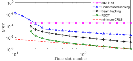
Figure 4: MSE vs. time-slot number in static scenarios.
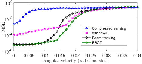
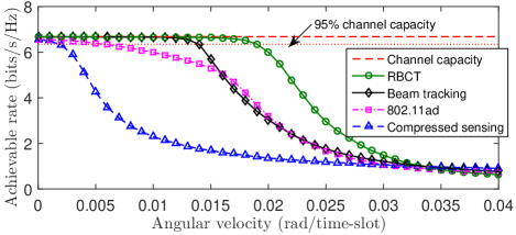
We compare the RBCT algorithm with three reference algorithms: the compressed sensing algorithm [13 ] , the IEEE 802.11ad algorithm [14 ] , and the beam tracking algorithm [18 ] . The first two algorithms have the same configuration as that in Section VI of [18 ] . The third one uses the same training beamforming vectors as the RBCT algorithm, i.e., in each time-slot, it receives two pilots with the beamforming vectors in (12 II M = 32 𝑀 32 M\!=\!32 d = 0.5 λ 𝑑 0.5 𝜆 d\!=\!0.5\lambda s = 1 + j 2 𝑠 1 𝑗 2 {s}\!=\!\frac{1+j}{2} | s | 2 σ 2 superscript 𝑠 2 superscript 𝜎 2 \frac{|{s}|^{2}}{\sigma^{2}} 5 dB 5 dB 5\text{dB}
In static scenarios, we set the step-size as a n = 1 n , n ≥ 1 formulae-sequence subscript 𝑎 𝑛 1 𝑛 𝑛 1 a_{n}\!=\!\frac{1}{n},n\!\geq\!1 θ 𝜃 \theta [ − 90 ∘ , 90 ∘ ] superscript 90 superscript 90 [-90^{\circ},90^{\circ}] 4 III-A
Figure 5: MSE vs. angular velocity in dynamic scenarios.Figure 6: Data rate vs. angular velocity in dynamic scenarios.
In dynamic scenarios, we set the step-size as a constant value, i.e., a n = 1 , n ≥ 1 formulae-sequence subscript 𝑎 𝑛 1 𝑛 1 a_{n}\!=\!1,n\!\geq\!1 θ n = θ n − 1 + δ n − 1 ⋅ ω subscript 𝜃 𝑛 subscript 𝜃 𝑛 1 ⋅ subscript 𝛿 𝑛 1 𝜔 \theta_{n}\!=\!\theta_{n-1}\!+\!\delta_{n-1}\!\cdot\!\omega θ 0 = 0 subscript 𝜃 0 0 \theta_{0}=0 δ n ∈ { − 1 , 1 } subscript 𝛿 𝑛 1 1 \delta_{n}\in\{-1,\!1\} ω ∈ [ 0 , 0.04 ] 𝜔 0 0.04 \omega\!\in\![0,0.04] δ n subscript 𝛿 𝑛 \delta_{n} θ n subscript 𝜃 𝑛 \theta_{n} [ − π 3 , π 3 ] 𝜋 3 𝜋 3 [-\frac{\pi}{3},\!\frac{\pi}{3}] β n ( 𝔼 [ | β n | 2 ] = 1 ) subscript 𝛽 𝑛 𝔼 delimited-[] superscript subscript 𝛽 𝑛 2 1 \beta_{n}(\mathbb{E}\left[|\beta_{n}|^{2}\right]\!=\!1) κ = 15 dB 𝜅 15 dB \kappa\!=\!15\text{dB} [23 ] . In Fig. 5 6 6
Appendix A Proof of Theorem 1
Before providing the proof, let us provide some useful definitions. In static beam tracking, where 𝝍 n = 𝝍 = [ β re , β im , x ] T subscript 𝝍 𝑛 𝝍 superscript superscript 𝛽 re superscript 𝛽 im 𝑥
T \boldsymbol{\psi}_{n}\!=\!\boldsymbol{\psi}\!=\![\beta^{\text{re}},\!\beta^{\text{im}},\!x]^{\text{T}} 𝒮 n = 𝒮 = Δ { 𝝍 ^ n − 1 : 𝐟 ( 𝝍 ^ n − 1 , 𝝍 ) = 𝟎 , ∂ 𝐟 ( 𝝍 ^ n − 1 , 𝝍 ) ∂ 𝝍 ^ n − 1 T ≺ 0 } subscript 𝒮 𝑛 𝒮 Δ conditional-set subscript ^ 𝝍 𝑛 1 formulae-sequence 𝐟 subscript ^ 𝝍 𝑛 1 𝝍 0 precedes 𝐟 subscript ^ 𝝍 𝑛 1 𝝍 superscript subscript ^ 𝝍 𝑛 1 T 0 \mathcal{S}_{n}\!=\!\mathcal{S}\!\overset{\Delta}{=}\!\Big{\{}\hat{\boldsymbol{\psi}}_{n-1}\!:\!\mathbf{f}\left(\hat{\boldsymbol{\psi}}_{n-1},\boldsymbol{\psi}\right)\!=\!\mathbf{0},\frac{\partial\mathbf{f}\left(\hat{\boldsymbol{\psi}}_{n-1},\boldsymbol{\psi}\right)}{\partial\hat{\boldsymbol{\psi}}_{n-1}^{\text{T}}}\prec 0\Big{\}} 19
𝝍 ^ n = 𝝍 ^ n − 1 + a n ( 𝐟 ( 𝝍 ^ n − 1 , 𝝍 ) + 𝐳 ^ n ) , subscript ^ 𝝍 𝑛 subscript ^ 𝝍 𝑛 1 subscript 𝑎 𝑛 𝐟 subscript ^ 𝝍 𝑛 1 𝝍 subscript ^ 𝐳 𝑛 \displaystyle\hat{\boldsymbol{\psi}}_{n}=\hat{\boldsymbol{\psi}}_{n\!-\!1}+a_{n}\left(\mathbf{f}\left(\hat{\boldsymbol{\psi}}_{n-1},\boldsymbol{\psi}\right)+\hat{\mathbf{z}}_{n}\right), (29)
where 𝐟 ( 𝝍 ^ n − 1 , 𝝍 ) 𝐟 subscript ^ 𝝍 𝑛 1 𝝍 \mathbf{f}\left(\hat{\boldsymbol{\psi}}_{n-1},\boldsymbol{\psi}\right) 𝐳 ^ n subscript ^ 𝐳 𝑛 \hat{\mathbf{z}}_{n} 20 21 21
𝐳 ^ n ∼ 𝒩 ( 𝟎 , 𝐈 ( 𝝍 ^ n − 1 , 𝐖 n ) − 1 ) , similar-to subscript ^ 𝐳 𝑛 𝒩 0 𝐈 superscript subscript ^ 𝝍 𝑛 1 subscript 𝐖 𝑛 1 \displaystyle\hat{\mathbf{z}}_{n}\sim\mathcal{N}\left(\mathbf{0},\mathbf{I}(\hat{\boldsymbol{\psi}}_{n\!-\!1},\!\mathbf{W}_{n})^{-1}\right), (30)
where 𝔼 [ 𝐳 ^ n ] = 𝟎 𝔼 delimited-[] subscript ^ 𝐳 𝑛 0 \mathbb{E}\left[\hat{\mathbf{z}}_{n}\right]=\mathbf{0} 𝐈 ( 𝝍 ^ n − 1 , 𝐖 n ) − 1 𝐈 superscript subscript ^ 𝝍 𝑛 1 subscript 𝐖 𝑛 1 \mathbf{I}(\hat{\boldsymbol{\psi}}_{n\!-\!1},\!\mathbf{W}_{n})^{-1} 𝐳 ^ n subscript ^ 𝐳 𝑛 \hat{\mathbf{z}}_{n} 31 31 ( a ) 𝑎 (a)
𝔼 [ ( 𝐳 ^ n − 𝔼 [ 𝐳 ^ n ] ) ( 𝐳 ^ n − 𝔼 [ 𝐳 ^ n ] ) T ] = 𝔼 delimited-[] subscript ^ 𝐳 𝑛 𝔼 delimited-[] subscript ^ 𝐳 𝑛 superscript subscript ^ 𝐳 𝑛 𝔼 delimited-[] subscript ^ 𝐳 𝑛 T absent \displaystyle\mathbb{E}\left[\left(\hat{\mathbf{z}}_{n}-\mathbb{E}\left[\hat{\mathbf{z}}_{n}\right]\right)\left(\hat{\mathbf{z}}_{n}-\mathbb{E}\left[\hat{\mathbf{z}}_{n}\right]\right)^{\text{T}}\right]= 4 σ 0 4 𝐈 ( 𝝍 ^ n − 1 , 𝐖 n ) − 1 ⋅ 𝔼 { [ Re { s H 𝐠 ^ n H 𝐳 n } Im { s H 𝐠 ^ n H 𝐳 n } Re { s H 𝐞 ^ n H 𝐳 n } ] ⋅ [ Re { s H 𝐠 ^ n H 𝐳 n } Im { s H 𝐠 ^ n H 𝐳 n } Re { s H 𝐞 ^ n H 𝐳 n } ] T } ⋅ 𝐈 ( 𝝍 ^ n − 1 , 𝐖 n ) − 1 ⋅ ⋅ 4 superscript subscript 𝜎 0 4 𝐈 superscript subscript ^ 𝝍 𝑛 1 subscript 𝐖 𝑛 1 𝔼 ⋅ delimited-[] matrix Re superscript 𝑠 H superscript subscript ^ 𝐠 𝑛 H subscript 𝐳 𝑛 Im superscript 𝑠 H superscript subscript ^ 𝐠 𝑛 H subscript 𝐳 𝑛 Re superscript 𝑠 H superscript subscript ^ 𝐞 𝑛 H subscript 𝐳 𝑛 superscript delimited-[] matrix Re superscript 𝑠 H superscript subscript ^ 𝐠 𝑛 H subscript 𝐳 𝑛 Im superscript 𝑠 H superscript subscript ^ 𝐠 𝑛 H subscript 𝐳 𝑛 Re superscript 𝑠 H superscript subscript ^ 𝐞 𝑛 H subscript 𝐳 𝑛 T 𝐈 superscript subscript ^ 𝝍 𝑛 1 subscript 𝐖 𝑛 1 \displaystyle~{}\frac{4}{\sigma_{0}^{4}}\mathbf{I}(\hat{\boldsymbol{\psi}}_{n\!-\!1},\!\mathbf{W}_{n})^{-1}\!\cdot\!\mathbb{E}\!\left\{\!\!\left[\begin{matrix}\operatorname{Re}\{{s}^{\text{H}}\hat{\mathbf{g}}_{n}^{\text{H}}\mathbf{z}_{n}\}\\
\operatorname{Im}\{{s}^{\text{H}}\hat{\mathbf{g}}_{n}^{\text{H}}\mathbf{z}_{n}\}\\
\operatorname{Re}\{{s}^{\text{H}}\hat{\mathbf{e}}_{n}^{\text{H}}\mathbf{z}_{n}\}\end{matrix}\right]\!\!\cdot\!\!\left[\begin{matrix}\operatorname{Re}\{{s}^{\text{H}}\hat{\mathbf{g}}_{n}^{\text{H}}\mathbf{z}_{n}\}\\
\operatorname{Im}\{{s}^{\text{H}}\hat{\mathbf{g}}_{n}^{\text{H}}\mathbf{z}_{n}\}\\
\operatorname{Re}\{{s}^{\text{H}}\hat{\mathbf{e}}_{n}^{\text{H}}\mathbf{z}_{n}\}\end{matrix}\right]^{\text{\!\!T}}\!\right\}\!\cdot\!\mathbf{I}(\hat{\boldsymbol{\psi}}_{n\!-\!1},\!\mathbf{W}_{n})^{-1} (31)
= ( a ) 𝑎 \displaystyle\overset{(a)}{=} 𝐈 ( 𝝍 ^ n − 1 , 𝐖 n ) − 1 . 𝐈 superscript subscript ^ 𝝍 𝑛 1 subscript 𝐖 𝑛 1 \displaystyle~{}\mathbf{I}(\hat{\boldsymbol{\psi}}_{n\!-\!1},\!\mathbf{W}_{n})^{-1}.
•
Since 𝐳 n = [ z n , 1 , z n , 2 ] T subscript 𝐳 𝑛 superscript subscript 𝑧 𝑛 1
subscript 𝑧 𝑛 2
T \mathbf{z}_{n}\!=\!\left[z_{n,1},z_{n,2}\right]^{\text{T}} i.i.d. circularly symmetric complex Gaussian random variables, we get
s H 𝐠 ^ n H 𝐳 n ∼ 𝒞 𝒩 ( 0 , ‖ s 𝐠 ^ n ‖ 2 2 σ 0 2 ) , similar-to superscript 𝑠 H superscript subscript ^ 𝐠 𝑛 H subscript 𝐳 𝑛 𝒞 𝒩 0 superscript subscript norm 𝑠 subscript ^ 𝐠 𝑛 2 2 superscript subscript 𝜎 0 2 \displaystyle{s}^{\text{H}}\hat{\mathbf{g}}_{n}^{\text{H}}\mathbf{z}_{n}\sim\mathcal{CN}\left(0,\left\|{s}\hat{\mathbf{g}}_{n}\right\|_{2}^{2}\sigma_{0}^{2}\right), (32)
and
s H 𝐞 ^ n H 𝐳 n ∼ 𝒞 𝒩 ( 0 , ‖ s 𝐞 ^ n ‖ 2 2 σ 0 2 ) . similar-to superscript 𝑠 H superscript subscript ^ 𝐞 𝑛 H subscript 𝐳 𝑛 𝒞 𝒩 0 superscript subscript norm 𝑠 subscript ^ 𝐞 𝑛 2 2 superscript subscript 𝜎 0 2 \displaystyle{s}^{\text{H}}\hat{\mathbf{e}}_{n}^{\text{H}}\mathbf{z}_{n}\sim\mathcal{CN}\left(0,\left\|{s}\hat{\mathbf{e}}_{n}\right\|_{2}^{2}\sigma_{0}^{2}\right). (33)
•
By splitting the real part and imaginary part, we obtain
{ Re { s H 𝐠 ^ n H 𝐳 n } = Re { s H 𝐠 ^ n H } Re { 𝐳 n } − Im { s H 𝐠 ^ n H } Im { 𝐳 n } , Im { s H 𝐠 ^ n H 𝐳 n } = Re { s H 𝐠 ^ n H } Im { 𝐳 n } + Im { s H 𝐠 ^ n H } Re { 𝐳 n } , Re { s H 𝐞 ^ n H 𝐳 n } = Re { s H 𝐞 ^ n H } Re { 𝐳 n } − Im { s H 𝐞 ^ n H } Im { 𝐳 n } , Re { s H 𝐠 ^ n H s 𝐞 ^ n } = | s | 2 Re { 𝐠 ^ n H 𝐞 ^ n } = Re { s H 𝐠 ^ n H } Re { s 𝐞 ^ n } − Im { s H 𝐠 ^ n H } Im { s 𝐞 ^ n } , Im { s H 𝐠 ^ n H s 𝐞 ^ n } = | s | 2 Im { 𝐠 ^ n H 𝐞 ^ n } = Re { s H 𝐠 ^ n H } Im { s 𝐞 ^ n } + Im { s H 𝐠 ^ n H } Re { s 𝐞 ^ n } . \!\!\!\!\!\!\!\!\!\left\{\begin{aligned} &\operatorname{Re}\{{s}^{\text{H}}\hat{\mathbf{g}}_{n}^{\text{H}}\mathbf{z}_{n}\}\!=\!\operatorname{Re}\{{s}^{\text{H}}\hat{\mathbf{g}}_{n}^{\text{H}}\}\operatorname{Re}\{\mathbf{z}_{n}\}\!-\!\operatorname{Im}\{{s}^{\text{H}}\hat{\mathbf{g}}_{n}^{\text{H}}\}\operatorname{Im}\{\mathbf{z}_{n}\},\\
&\operatorname{Im}\{{s}^{\text{H}}\hat{\mathbf{g}}_{n}^{\text{H}}\mathbf{z}_{n}\}\!=\!\operatorname{Re}\{{s}^{\text{H}}\hat{\mathbf{g}}_{n}^{\text{H}}\}\operatorname{Im}\{\mathbf{z}_{n}\}\!+\!\operatorname{Im}\{{s}^{\text{H}}\hat{\mathbf{g}}_{n}^{\text{H}}\}\operatorname{Re}\{\mathbf{z}_{n}\},\\
&\operatorname{Re}\{{s}^{\text{H}}\hat{\mathbf{e}}_{n}^{\text{H}}\mathbf{z}_{n}\}\!=\!\operatorname{Re}\{{s}^{\text{H}}\hat{\mathbf{e}}_{n}^{\text{H}}\}\operatorname{Re}\{\mathbf{z}_{n}\}\!-\!\operatorname{Im}\{{s}^{\text{H}}\hat{\mathbf{e}}_{n}^{\text{H}}\}\operatorname{Im}\{\mathbf{z}_{n}\},\\
&\operatorname{Re}\{{s}^{\text{H}}\hat{\mathbf{g}}_{n}^{\text{H}}{s}\hat{\mathbf{e}}_{n}\}\!=\!|{s}|^{2}\operatorname{Re}\{\hat{\mathbf{g}}_{n}^{\text{H}}\hat{\mathbf{e}}_{n}\}\\
&~{}~{}~{}~{}~{}~{}~{}~{}~{}~{}\!=\operatorname{Re}\{{s}^{\text{H}}\hat{\mathbf{g}}_{n}^{\text{H}}\}\operatorname{Re}\{{s}\hat{\mathbf{e}}_{n}\}\!-\!\operatorname{Im}\{{s}^{\text{H}}\hat{\mathbf{g}}_{n}^{\text{H}}\}\operatorname{Im}\{{s}\hat{\mathbf{e}}_{n}\},\\
&\operatorname{Im}\{{s}^{\text{H}}\hat{\mathbf{g}}_{n}^{\text{H}}{s}\hat{\mathbf{e}}_{n}\}\!=\!|{s}|^{2}\operatorname{Im}\{\hat{\mathbf{g}}_{n}^{\text{H}}\hat{\mathbf{e}}_{n}\}\\
&~{}~{}~{}~{}~{}~{}~{}~{}~{}~{}\!=\operatorname{Re}\{{s}^{\text{H}}\hat{\mathbf{g}}_{n}^{\text{H}}\}\operatorname{Im}\{{s}\hat{\mathbf{e}}_{n}\}\!+\!\operatorname{Im}\{{s}^{\text{H}}\hat{\mathbf{g}}_{n}^{\text{H}}\}\operatorname{Re}\{{s}\hat{\mathbf{e}}_{n}\}.\end{aligned}\right.\!\!\!\!\! (34)
•
Combining (32 33 34
{ 𝔼 [ Re { s H 𝐠 ^ n H 𝐳 n } 2 ] = 𝔼 [ Im { s H 𝐠 ^ n H 𝐳 n } 2 ] = | s | 2 σ 0 2 2 ∥ 𝐠 ^ n ∥ 2 2 , 𝔼 [ Re { s H 𝐞 ^ n H 𝐳 n } 2 ] = | s | 2 σ 0 2 2 ∥ 𝐞 ^ n ∥ 2 2 , 𝔼 [ Re { s H 𝐠 ^ n H 𝐳 n } ⋅ Im { s H 𝐠 ^ n H 𝐳 n } ] = 0 , 𝔼 [ Re { s H 𝐠 ^ n H 𝐳 n } ⋅ Re { s H 𝐞 ^ n H 𝐳 n } ] = | s | 2 σ 0 2 2 Re { 𝐠 ^ n H 𝐞 ^ n } , 𝔼 [ Im { s H 𝐠 ^ n H 𝐳 n } ⋅ Re { s H 𝐞 ^ n H 𝐳 n } ] = | s | 2 σ 0 2 2 Im { 𝐠 ^ n H 𝐞 ^ n } . \!\!\!\!\!\!\left\{\begin{aligned} &\mathbb{E}\left[\operatorname{Re}\{{s}^{\text{H}}\hat{\mathbf{g}}_{n}^{\text{H}}\mathbf{z}_{n}\}^{2}\right]\!=\!\mathbb{E}\left[\operatorname{Im}\{{s}^{\text{H}}\hat{\mathbf{g}}_{n}^{\text{H}}\mathbf{z}_{n}\}^{2}\right]\!=\!\frac{|{s}|^{2}\sigma_{0}^{2}}{2}\left\|\hat{\mathbf{g}}_{n}\right\|_{2}^{2},\\
&\mathbb{E}\left[\operatorname{Re}\{{s}^{\text{H}}\hat{\mathbf{e}}_{n}^{\text{H}}\mathbf{z}_{n}\}^{2}\right]\!=\!\frac{|{s}|^{2}\sigma_{0}^{2}}{2}\left\|\hat{\mathbf{e}}_{n}\right\|_{2}^{2},\\
&\mathbb{E}\left[\operatorname{Re}\{{s}^{\text{H}}\hat{\mathbf{g}}_{n}^{\text{H}}\mathbf{z}_{n}\}\!\cdot\!\operatorname{Im}\{{s}^{\text{H}}\hat{\mathbf{g}}_{n}^{\text{H}}\mathbf{z}_{n}\}\right]=0,\\
&\mathbb{E}\left[\operatorname{Re}\{{s}^{\text{H}}\hat{\mathbf{g}}_{n}^{\text{H}}\mathbf{z}_{n}\}\!\cdot\!\operatorname{Re}\{{s}^{\text{H}}\hat{\mathbf{e}}_{n}^{\text{H}}\mathbf{z}_{n}\}\right]=\frac{|{s}|^{2}\sigma_{0}^{2}}{2}\operatorname{Re}\{\hat{\mathbf{g}}_{n}^{\text{H}}\hat{\mathbf{e}}_{n}\},\\
&\mathbb{E}\left[\operatorname{Im}\{{s}^{\text{H}}\hat{\mathbf{g}}_{n}^{\text{H}}\mathbf{z}_{n}\}\!\cdot\!\operatorname{Re}\{{s}^{\text{H}}\hat{\mathbf{e}}_{n}^{\text{H}}\mathbf{z}_{n}\}\right]=\frac{|{s}|^{2}\sigma_{0}^{2}}{2}\operatorname{Im}\{\hat{\mathbf{g}}_{n}^{\text{H}}\hat{\mathbf{e}}_{n}\}.\end{aligned}\right.\!\!\!\!\! (35)
Hence, we have
𝔼 { [ Re { s H 𝐠 ^ n H 𝐳 n } Im { s H 𝐠 ^ n H 𝐳 n } Re { s H 𝐞 ^ n H 𝐳 n } ] ⋅ [ Re { s H 𝐠 ^ n H 𝐳 n } Im { s H 𝐠 ^ n H 𝐳 n } Re { s H 𝐞 ^ n H 𝐳 n } ] T } = σ 0 4 4 𝐈 ( 𝝍 ^ n − 1 , 𝐖 n ) . 𝔼 ⋅ delimited-[] matrix Re superscript 𝑠 H superscript subscript ^ 𝐠 𝑛 H subscript 𝐳 𝑛 Im superscript 𝑠 H superscript subscript ^ 𝐠 𝑛 H subscript 𝐳 𝑛 Re superscript 𝑠 H superscript subscript ^ 𝐞 𝑛 H subscript 𝐳 𝑛 superscript delimited-[] matrix Re superscript 𝑠 H superscript subscript ^ 𝐠 𝑛 H subscript 𝐳 𝑛 Im superscript 𝑠 H superscript subscript ^ 𝐠 𝑛 H subscript 𝐳 𝑛 Re superscript 𝑠 H superscript subscript ^ 𝐞 𝑛 H subscript 𝐳 𝑛 T superscript subscript 𝜎 0 4 4 𝐈 subscript ^ 𝝍 𝑛 1 subscript 𝐖 𝑛 \displaystyle\mathbb{E}\!\left\{\!\!\left[\begin{matrix}\operatorname{Re}\{{s}^{\text{H}}\hat{\mathbf{g}}_{n}^{\text{H}}\mathbf{z}_{n}\}\\
\operatorname{Im}\{{s}^{\text{H}}\hat{\mathbf{g}}_{n}^{\text{H}}\mathbf{z}_{n}\}\\
\operatorname{Re}\{{s}^{\text{H}}\hat{\mathbf{e}}_{n}^{\text{H}}\mathbf{z}_{n}\}\end{matrix}\right]\!\!\cdot\!\!\left[\begin{matrix}\operatorname{Re}\{{s}^{\text{H}}\hat{\mathbf{g}}_{n}^{\text{H}}\mathbf{z}_{n}\}\\
\operatorname{Im}\{{s}^{\text{H}}\hat{\mathbf{g}}_{n}^{\text{H}}\mathbf{z}_{n}\}\\
\operatorname{Re}\{{s}^{\text{H}}\hat{\mathbf{e}}_{n}^{\text{H}}\mathbf{z}_{n}\}\end{matrix}\right]^{\text{\!\!T}}\!\right\}\!=\!\frac{\sigma_{0}^{4}}{4}\mathbf{I}(\hat{\boldsymbol{\psi}}_{n\!-\!1},\!\mathbf{W}_{n}). (36)
•
Plugging (36 31 ( a ) 𝑎 (a)
Let { 𝒢 n : n ≥ 0 } conditional-set subscript 𝒢 𝑛 𝑛 0 \{\mathcal{G}_{n}:n\geq 0\} σ 𝜎 \sigma { 𝝍 ^ 0 , 𝝍 ^ 1 , 𝝍 ^ 2 , … } subscript ^ 𝝍 0 subscript ^ 𝝍 1 subscript ^ 𝝍 2 … \{\hat{\boldsymbol{\psi}}_{0},\hat{\boldsymbol{\psi}}_{1},\hat{\boldsymbol{\psi}}_{2},\ldots\} 𝒢 n − 1 ⊂ 𝒢 n subscript 𝒢 𝑛 1 subscript 𝒢 𝑛 \mathcal{G}_{n-1}\!\subset\!\mathcal{G}_{n} 𝒢 0 = Δ σ ( 𝝍 ^ 0 ) subscript 𝒢 0 Δ 𝜎 subscript ^ 𝝍 0 \mathcal{G}_{0}\!\overset{\Delta}{=}\!\sigma(\hat{\boldsymbol{\psi}}_{0}) 𝒢 n = Δ σ ( 𝝍 ^ 0 , 𝐳 ^ 1 , … , 𝐳 ^ n ) subscript 𝒢 𝑛 Δ 𝜎 subscript ^ 𝝍 0 subscript ^ 𝐳 1 … subscript ^ 𝐳 𝑛 \mathcal{G}_{n}\!\overset{\Delta}{=}\!\sigma(\hat{\boldsymbol{\psi}}_{0},\hat{\mathbf{z}}_{1},\ldots,\hat{\mathbf{z}}_{n}) n ≥ 1 𝑛 1 n\geq 1 𝐳 ^ n subscript ^ 𝐳 𝑛 \hat{\mathbf{z}}_{n} i.i.d. circularly symmetric complex Gaussian random variables with zero mean, 𝐳 ^ n subscript ^ 𝐳 𝑛 \hat{\mathbf{z}}_{n} 𝒢 n − 1 subscript 𝒢 𝑛 1 \mathcal{G}_{n-1} 𝝍 ^ n − 1 ∈ 𝒢 n − 1 subscript ^ 𝝍 𝑛 1 subscript 𝒢 𝑛 1 \hat{\boldsymbol{\psi}}_{n-1}\!\in\!\mathcal{G}_{n-1}
𝔼 [ 𝐟 ( 𝝍 ^ n − 1 , 𝝍 ) + 𝐳 ^ n | 𝒢 n − 1 ] 𝔼 delimited-[] 𝐟 subscript ^ 𝝍 𝑛 1 𝝍 conditional subscript ^ 𝐳 𝑛 subscript 𝒢 𝑛 1 \displaystyle~{}\mathbb{E}\left[\left.\mathbf{f}\left(\hat{\boldsymbol{\psi}}_{n-1},\boldsymbol{\psi}\right)+\hat{\mathbf{z}}_{n}\right|\mathcal{G}_{n-1}\right] (37)
= \displaystyle= 𝔼 [ 𝐟 ( 𝝍 ^ n − 1 , 𝝍 ) | 𝒢 n − 1 ] + 𝔼 [ 𝐳 ^ n | 𝒢 n − 1 ] = 𝐟 ( 𝝍 ^ n − 1 , 𝝍 ) , 𝔼 delimited-[] conditional 𝐟 subscript ^ 𝝍 𝑛 1 𝝍 subscript 𝒢 𝑛 1 𝔼 delimited-[] conditional subscript ^ 𝐳 𝑛 subscript 𝒢 𝑛 1 𝐟 subscript ^ 𝝍 𝑛 1 𝝍 \displaystyle~{}\mathbb{E}\left[\left.\mathbf{f}\left(\hat{\boldsymbol{\psi}}_{n-1},\boldsymbol{\psi}\right)\right|\mathcal{G}_{n-1}\right]+\mathbb{E}\left[\left.\hat{\mathbf{z}}_{n}\right|\mathcal{G}_{n-1}\right]=\mathbf{f}\left(\hat{\boldsymbol{\psi}}_{n-1},\boldsymbol{\psi}\right),
for n ≥ 1 𝑛 1 n\geq 1
Theorem 5.2.1 in [21 , Section 5.2.1] provided the sufficient conditions under which x ^ n subscript ^ 𝑥 𝑛 \hat{x}_{n} a n subscript 𝑎 𝑛 a_{n} 26 α > 0 𝛼 0 \alpha>0 N 0 ≥ 0 subscript 𝑁 0 0 N_{0}\geq 0
1)
Step-size requirements:
{ a n = α n + N 0 → 0 , ∑ n = 1 ∞ a n = ∑ n = 1 ∞ α n + N 0 = ∞ , ∑ n = 1 ∞ a n 2 = ∑ n = 1 ∞ α 2 ( n + N 0 ) 2 ≤ ∑ i = 1 ∞ α 2 i 2 < ∞ . \left\{\begin{aligned} &a_{n}=\frac{\alpha}{n+N_{0}}\rightarrow 0,\\
&\sum\limits_{n=1}^{\infty}a_{n}=\sum\limits_{n=1}^{\infty}\frac{\alpha}{n+N_{0}}=\infty,\\
&\sum\limits_{n=1}^{\infty}a_{n}^{2}=\sum\limits_{n=1}^{\infty}\frac{\alpha^{2}}{(n+N_{0})^{2}}\leq\sum\limits_{i=1}^{\infty}\frac{\alpha^{2}}{i^{2}}<\infty.\end{aligned}\right. (38)
2)
We need to prove that sup n 𝔼 [ ‖ 𝐟 ( 𝝍 ^ n − 1 , 𝝍 ) + 𝐳 ^ n ‖ 2 2 ] < ∞ subscript supremum 𝑛 𝔼 delimited-[] superscript subscript norm 𝐟 subscript ^ 𝝍 𝑛 1 𝝍 subscript ^ 𝐳 𝑛 2 2 \sup\nolimits_{n}\mathbb{E}\left[\left\|\mathbf{f}\left(\hat{\boldsymbol{\psi}}_{n-1},\boldsymbol{\psi}\right)+\hat{\mathbf{z}}_{n}\right\|_{2}^{2}\right]<\infty 29 30
𝔼 [ ‖ 𝐟 ( 𝝍 ^ n − 1 , 𝝍 ) + 𝐳 ^ n ‖ 2 2 ] 𝔼 delimited-[] superscript subscript norm 𝐟 subscript ^ 𝝍 𝑛 1 𝝍 subscript ^ 𝐳 𝑛 2 2 \displaystyle\mathbb{E}\left[\left\|\mathbf{f}\left(\hat{\boldsymbol{\psi}}_{n-1},\boldsymbol{\psi}\right)+\hat{\mathbf{z}}_{n}\right\|_{2}^{2}\right] (39)
= \displaystyle= 𝔼 [ ‖ 𝐟 ( 𝝍 ^ n − 1 , 𝝍 ) ‖ 2 2 + 2 𝐟 ( 𝝍 ^ n − 1 , 𝝍 ) T 𝐳 ^ n + ‖ 𝐳 ^ n ‖ 2 2 ] 𝔼 delimited-[] superscript subscript norm 𝐟 subscript ^ 𝝍 𝑛 1 𝝍 2 2 2 𝐟 superscript subscript ^ 𝝍 𝑛 1 𝝍 T subscript ^ 𝐳 𝑛 superscript subscript norm subscript ^ 𝐳 𝑛 2 2 \displaystyle\mathbb{E}\left[\left\|\mathbf{f}\left(\hat{\boldsymbol{\psi}}_{n-1},\boldsymbol{\psi}\right)\right\|_{2}^{2}+2\mathbf{f}\left(\hat{\boldsymbol{\psi}}_{n-1},\boldsymbol{\psi}\right)^{\text{T}}\hat{\mathbf{z}}_{n}+\left\|\hat{\mathbf{z}}_{n}\right\|_{2}^{2}\right]
= ( a ) 𝑎 \displaystyle\overset{(a)}{=} 𝔼 [ ‖ 𝐟 ( 𝝍 ^ n − 1 , 𝝍 ) ‖ 2 2 ] + tr ( 𝐈 ( 𝝍 ^ n − 1 , 𝐖 n ) − 1 ) , 𝔼 delimited-[] superscript subscript norm 𝐟 subscript ^ 𝝍 𝑛 1 𝝍 2 2 tr 𝐈 superscript subscript ^ 𝝍 𝑛 1 subscript 𝐖 𝑛 1 \displaystyle\mathbb{E}\left[\left\|\mathbf{f}\left(\hat{\boldsymbol{\psi}}_{n-1},\boldsymbol{\psi}\right)\right\|_{2}^{2}\right]+\operatorname{tr}\left(\mathbf{I}(\hat{\boldsymbol{\psi}}_{n\!-\!1},\!\mathbf{W}_{n})^{-1}\right),
where step ( a ) 𝑎 (a) 30 𝐳 ^ n subscript ^ 𝐳 𝑛 \hat{\mathbf{z}}_{n} 𝐟 ( 𝝍 ^ n − 1 , 𝝍 ) 𝐟 subscript ^ 𝝍 𝑛 1 𝝍 \mathbf{f}\left(\hat{\boldsymbol{\psi}}_{n-1},\boldsymbol{\psi}\right) 17 23
‖ 𝐟 ( 𝝍 ^ n − 1 , 𝝍 ) ‖ 2 2 ≤ superscript subscript norm 𝐟 subscript ^ 𝝍 𝑛 1 𝝍 2 2 absent \displaystyle\left\|\mathbf{f}\left(\hat{\boldsymbol{\psi}}_{n-1},\boldsymbol{\psi}\right)\right\|_{2}^{2}\leq ‖ 𝐈 ( 𝝍 ^ n − 1 , 𝐖 n ) − 1 ‖ F 2 superscript subscript norm 𝐈 superscript subscript ^ 𝝍 𝑛 1 subscript 𝐖 𝑛 1 F 2 \displaystyle~{}\left\|\mathbf{I}(\hat{\boldsymbol{\psi}}_{n\!-\!1},\!\mathbf{W}_{n})^{-1}\right\|_{\text{F}}^{2} (40)
⋅ ‖ 2 | s | 2 σ 0 2 [ Re { 𝐠 ^ n H ( β n 𝐖 n H 𝐚 ( x n ) − β ^ n − 1 𝐠 ^ n ) } Im { 𝐠 ^ n H ( β n 𝐖 n H 𝐚 ( x n ) − β ^ n − 1 𝐠 ^ n ) } Re { 𝐞 ^ n H ( β n 𝐖 n H 𝐚 ( x n ) − β ^ n − 1 𝐠 ^ n ) } ] ‖ 2 2 . ⋅ absent superscript subscript norm 2 superscript 𝑠 2 superscript subscript 𝜎 0 2 delimited-[] matrix Re superscript subscript ^ 𝐠 𝑛 H subscript 𝛽 𝑛 superscript subscript 𝐖 𝑛 H 𝐚 subscript 𝑥 𝑛 subscript ^ 𝛽 𝑛 1 subscript ^ 𝐠 𝑛 Im superscript subscript ^ 𝐠 𝑛 H subscript 𝛽 𝑛 superscript subscript 𝐖 𝑛 H 𝐚 subscript 𝑥 𝑛 subscript ^ 𝛽 𝑛 1 subscript ^ 𝐠 𝑛 Re superscript subscript ^ 𝐞 𝑛 H subscript 𝛽 𝑛 superscript subscript 𝐖 𝑛 H 𝐚 subscript 𝑥 𝑛 subscript ^ 𝛽 𝑛 1 subscript ^ 𝐠 𝑛 2 2 \displaystyle~{}\!\!\!\!\!\!\!\!\!\!\!\!\!\!\!\!\!\!\!\!\!\!\!\!\!\!\!\!\!\!\!\!\!\cdot\!\left\|\frac{2|{s}|^{2}}{\sigma_{0}^{2}}\!\!\left[\begin{matrix}\operatorname{Re}\{\hat{\mathbf{g}}_{n}^{\text{H}}(\beta_{n}\mathbf{W}_{n}^{\text{H}}\mathbf{a}(x_{n})\!-\!\hat{\beta}_{n\!-\!1}\hat{\mathbf{g}}_{n})\}\\
\operatorname{Im}\{\hat{\mathbf{g}}_{n}^{\text{H}}(\beta_{n}\mathbf{W}_{n}^{\text{H}}\mathbf{a}(x_{n})\!-\!\hat{\beta}_{n\!-\!1}\hat{\mathbf{g}}_{n})\}\\
\operatorname{Re}\{\hat{\mathbf{e}}_{n}^{\text{H}}(\beta_{n}\mathbf{W}_{n}^{\text{H}}\mathbf{a}(x_{n})\!-\!\hat{\beta}_{n\!-\!1}\hat{\mathbf{g}}_{n})\}\end{matrix}\right]\right\|_{2}^{2}.
Due to that the Fisher information matrix is invertible, we get
‖ 𝐈 ( 𝝍 ^ n − 1 , 𝐖 n ) − 1 ‖ F 2 < ∞ . superscript subscript norm 𝐈 superscript subscript ^ 𝝍 𝑛 1 subscript 𝐖 𝑛 1 F 2 \displaystyle\left\|\mathbf{I}(\hat{\boldsymbol{\psi}}_{n\!-\!1},\!\mathbf{W}_{n})^{-1}\right\|_{\text{F}}^{2}<\infty. (41)
In addition, since 𝐖 n = [ 𝐰 n , 1 , 𝐰 n , 2 ] subscript 𝐖 𝑛 subscript 𝐰 𝑛 1
subscript 𝐰 𝑛 2
\mathbf{W}_{n}\!=\!\left[\mathbf{w}_{n,1},\mathbf{w}_{n,2}\right] 𝐠 ^ n = 𝐖 n H 𝐚 ( x ^ n − 1 ) subscript ^ 𝐠 𝑛 superscript subscript 𝐖 𝑛 H 𝐚 subscript ^ 𝑥 𝑛 1 \hat{\mathbf{g}}_{n}\!=\!\mathbf{W}_{n}^{\text{H}}\mathbf{a}(\hat{x}_{n\!-\!1}) 𝐞 ^ n = β ^ n − 1 𝐖 n H 𝐚 ˙ ( x ^ n − 1 ) subscript ^ 𝐞 𝑛 subscript ^ 𝛽 𝑛 1 superscript subscript 𝐖 𝑛 H ˙ 𝐚 subscript ^ 𝑥 𝑛 1 \hat{\mathbf{e}}_{n}\!=\!\hat{\beta}_{n\!-\!1}\mathbf{W}_{n}^{\text{H}}\dot{\mathbf{a}}(\hat{x}_{n\!-\!1})
| 𝐰 n , i H 𝐚 ( x ) | superscript subscript 𝐰 𝑛 𝑖
H 𝐚 𝑥 \displaystyle\left|\mathbf{w}_{n,i}^{\text{H}}\mathbf{a}(x)\right| = | ∑ m = 1 M 1 M e − j ( 2 π d λ x − w m n , i ) | absent superscript subscript 𝑚 1 𝑀 1 𝑀 superscript 𝑒 𝑗 2 𝜋 𝑑 𝜆 𝑥 subscript 𝑤 𝑚 𝑛 𝑖
\displaystyle~{}=\left|\sum_{m=1}^{M}\frac{1}{\sqrt{M}}e^{-j(\frac{2\pi d}{\lambda}x-w_{mn,i})}\right| (42)
≤ ∑ m = 1 M 1 M | e − j ( 2 π d λ ( m − 1 ) x − w m n , i ) | absent superscript subscript 𝑚 1 𝑀 1 𝑀 superscript 𝑒 𝑗 2 𝜋 𝑑 𝜆 𝑚 1 𝑥 subscript 𝑤 𝑚 𝑛 𝑖
\displaystyle~{}\leq\sum_{m=1}^{M}\frac{1}{\sqrt{M}}\left|e^{-j(\frac{2\pi d}{\lambda}(m-1)x-w_{mn,i})}\right|
= M < ∞ , absent 𝑀 \displaystyle~{}=\sqrt{M}<\infty,
and
| 𝐰 n , i H 𝐚 ˙ ( x ) | superscript subscript 𝐰 𝑛 𝑖
H ˙ 𝐚 𝑥 \displaystyle\left|\mathbf{w}_{n,i}^{\text{H}}\dot{\mathbf{a}}(x)\right| = | ∑ m = 1 M − j 2 π d ( m − 1 ) λ M e − j ( 2 π d λ x − w m n , i ) | absent superscript subscript 𝑚 1 𝑀 𝑗 2 𝜋 𝑑 𝑚 1 𝜆 𝑀 superscript 𝑒 𝑗 2 𝜋 𝑑 𝜆 𝑥 subscript 𝑤 𝑚 𝑛 𝑖
\displaystyle~{}=\left|\sum_{m=1}^{M}-j\frac{2\pi d(m-1)}{\lambda\sqrt{M}}e^{-j(\frac{2\pi d}{\lambda}x-w_{mn,i})}\right|
≤ ∑ m = 1 M 2 π d ( m − 1 ) λ M | e − j ( 2 π d λ ( m − 1 ) x − w m n , i ) | absent superscript subscript 𝑚 1 𝑀 2 𝜋 𝑑 𝑚 1 𝜆 𝑀 superscript 𝑒 𝑗 2 𝜋 𝑑 𝜆 𝑚 1 𝑥 subscript 𝑤 𝑚 𝑛 𝑖
\displaystyle~{}\leq\sum_{m=1}^{M}\frac{2\pi d(m-1)}{\lambda\sqrt{M}}\left|e^{-j(\frac{2\pi d}{\lambda}(m-1)x-w_{mn,i})}\right|
= π d M ( M − 1 ) λ < ∞ , absent 𝜋 𝑑 𝑀 𝑀 1 𝜆 \displaystyle~{}=\frac{\pi d\sqrt{M}(M-1)}{\lambda}<\infty, (43)
for i = 1 , 2 𝑖 1 2
i=1,2 x 𝑥 x
‖ 2 | s | 2 σ 0 2 [ Re { 𝐠 ^ n H ( β n 𝐖 n H 𝐚 ( x n ) − β ^ n − 1 𝐠 ^ n ) } Im { 𝐠 ^ n H ( β n 𝐖 n H 𝐚 ( x n ) − β ^ n − 1 𝐠 ^ n ) } Re { 𝐞 ^ n H ( β n 𝐖 n H 𝐚 ( x n ) − β ^ n − 1 𝐠 ^ n ) } ] ‖ 2 2 < ∞ . superscript subscript norm 2 superscript 𝑠 2 superscript subscript 𝜎 0 2 delimited-[] matrix Re superscript subscript ^ 𝐠 𝑛 H subscript 𝛽 𝑛 superscript subscript 𝐖 𝑛 H 𝐚 subscript 𝑥 𝑛 subscript ^ 𝛽 𝑛 1 subscript ^ 𝐠 𝑛 Im superscript subscript ^ 𝐠 𝑛 H subscript 𝛽 𝑛 superscript subscript 𝐖 𝑛 H 𝐚 subscript 𝑥 𝑛 subscript ^ 𝛽 𝑛 1 subscript ^ 𝐠 𝑛 Re superscript subscript ^ 𝐞 𝑛 H subscript 𝛽 𝑛 superscript subscript 𝐖 𝑛 H 𝐚 subscript 𝑥 𝑛 subscript ^ 𝛽 𝑛 1 subscript ^ 𝐠 𝑛 2 2 \displaystyle\!\!\!\left\|\frac{2|{s}|^{2}}{\sigma_{0}^{2}}\!\!\left[\begin{matrix}\operatorname{Re}\{\hat{\mathbf{g}}_{n}^{\text{H}}(\beta_{n}\mathbf{W}_{n}^{\text{H}}\mathbf{a}(x_{n})\!-\!\hat{\beta}_{n\!-\!1}\hat{\mathbf{g}}_{n})\}\\
\operatorname{Im}\{\hat{\mathbf{g}}_{n}^{\text{H}}(\beta_{n}\mathbf{W}_{n}^{\text{H}}\mathbf{a}(x_{n})\!-\!\hat{\beta}_{n\!-\!1}\hat{\mathbf{g}}_{n})\}\\
\operatorname{Re}\{\hat{\mathbf{e}}_{n}^{\text{H}}(\beta_{n}\mathbf{W}_{n}^{\text{H}}\mathbf{a}(x_{n})\!-\!\hat{\beta}_{n\!-\!1}\hat{\mathbf{g}}_{n})\}\end{matrix}\right]\right\|_{2}^{2}\!<\!\infty.\!\!\! (44)
Hence, combining (41 44
𝔼 [ ‖ 𝐟 ( 𝝍 ^ n − 1 , 𝝍 ) ‖ 2 2 ] < ∞ . 𝔼 delimited-[] superscript subscript norm 𝐟 subscript ^ 𝝍 𝑛 1 𝝍 2 2 \displaystyle\mathbb{E}\left[\left\|\mathbf{f}\left(\hat{\boldsymbol{\psi}}_{n-1},\boldsymbol{\psi}\right)\right\|_{2}^{2}\right]<\infty. (45)
From (41 tr ( 𝐈 ( 𝝍 ^ n − 1 , 𝐖 n ) − 1 ) < ∞ tr 𝐈 superscript subscript ^ 𝝍 𝑛 1 subscript 𝐖 𝑛 1 \operatorname{tr}\left(\mathbf{I}(\hat{\boldsymbol{\psi}}_{n\!-\!1},\!\mathbf{W}_{n})^{-1}\right)<\infty
sup n 𝔼 [ ‖ 𝐟 ( 𝝍 ^ n − 1 , 𝝍 ) + 𝐳 ^ n ‖ 2 2 ] < ∞ . subscript supremum 𝑛 𝔼 delimited-[] superscript subscript norm 𝐟 subscript ^ 𝝍 𝑛 1 𝝍 subscript ^ 𝐳 𝑛 2 2 \displaystyle\sup\nolimits_{n}\mathbb{E}\left[\left\|\mathbf{f}\left(\hat{\boldsymbol{\psi}}_{n-1},\boldsymbol{\psi}\right)+\hat{\mathbf{z}}_{n}\right\|_{2}^{2}\right]<\infty. (46)
3)
The function 𝐟 ( 𝝍 ^ n − 1 , 𝝍 ) 𝐟 subscript ^ 𝝍 𝑛 1 𝝍 \mathbf{f}\left(\hat{\boldsymbol{\psi}}_{n-1},\boldsymbol{\psi}\right) 𝝍 ^ n − 1 subscript ^ 𝝍 𝑛 1 \hat{\boldsymbol{\psi}}_{n-1} 12
𝐖 n H 𝐚 ( x ) = [ ∑ m = 1 M 1 M e − j 2 π d λ ( m − 1 ) ( x − x ^ n − 1 + δ ∗ ) ∑ m = 1 M 1 M e − j 2 π d λ ( m − 1 ) ( x − x ^ n − 1 − δ ∗ ) ] . superscript subscript 𝐖 𝑛 H 𝐚 𝑥 delimited-[] matrix superscript subscript 𝑚 1 𝑀 1 𝑀 superscript 𝑒 𝑗 2 𝜋 𝑑 𝜆 𝑚 1 𝑥 subscript ^ 𝑥 𝑛 1 superscript 𝛿 superscript subscript 𝑚 1 𝑀 1 𝑀 superscript 𝑒 𝑗 2 𝜋 𝑑 𝜆 𝑚 1 𝑥 subscript ^ 𝑥 𝑛 1 superscript 𝛿 \displaystyle\!\!\!\!\mathbf{W}_{n}^{\text{H}}\mathbf{a}(x)\!=\!\left[\begin{matrix}\sum_{m=1}^{M}\frac{1}{\sqrt{M}}e^{-j\frac{2\pi d}{\lambda}(m-1)(x-\hat{x}_{n-1}+\delta^{*})}\\
\sum_{m=1}^{M}\frac{1}{\sqrt{M}}e^{-j\frac{2\pi d}{\lambda}(m-1)(x-\hat{x}_{n-1}-\delta^{*})}\end{matrix}\right]\!\!.\!\!\! (47)
Since e − j 2 π d λ ( m − 1 ) ( x − x ^ n − 1 ± δ ∗ ) superscript 𝑒 𝑗 2 𝜋 𝑑 𝜆 𝑚 1 plus-or-minus 𝑥 subscript ^ 𝑥 𝑛 1 superscript 𝛿 e^{-j\frac{2\pi d}{\lambda}(m-1)(x-\hat{x}_{n-1}\pm\delta^{*})} x ^ n − 1 subscript ^ 𝑥 𝑛 1 \hat{x}_{n-1} 𝐖 n H 𝐚 ( x ) superscript subscript 𝐖 𝑛 H 𝐚 𝑥 \mathbf{W}_{n}^{\text{H}}\mathbf{a}(x) e − j 2 π d λ ( m − 1 ) ( x − x ^ n − 1 ± δ ∗ ) , m = 1 , … , M formulae-sequence superscript 𝑒 𝑗 2 𝜋 𝑑 𝜆 𝑚 1 plus-or-minus 𝑥 subscript ^ 𝑥 𝑛 1 superscript 𝛿 𝑚
1 … 𝑀
e^{-j\frac{2\pi d}{\lambda}(m-1)(x-\hat{x}_{n-1}\pm\delta^{*})},m=1,\ldots,M 𝐖 n H 𝐚 ( x ) superscript subscript 𝐖 𝑛 H 𝐚 𝑥 \mathbf{W}_{n}^{\text{H}}\mathbf{a}(x) 𝝍 ^ n − 1 = [ β ^ n − 1 re , β ^ n − 1 im , x ^ n − 1 ] T subscript ^ 𝝍 𝑛 1 superscript subscript superscript ^ 𝛽 re 𝑛 1 subscript superscript ^ 𝛽 im 𝑛 1 subscript ^ 𝑥 𝑛 1
T \hat{\boldsymbol{\psi}}_{n-1}\!=\![\hat{\beta}^{\text{re}}_{n-1},\hat{\beta}^{\text{im}}_{n-1},\hat{x}_{n-1}]^{\text{T}} 𝐠 ^ n = 𝐖 n H 𝐚 ( x ^ n − 1 ) subscript ^ 𝐠 𝑛 superscript subscript 𝐖 𝑛 H 𝐚 subscript ^ 𝑥 𝑛 1 \hat{\mathbf{g}}_{n}\!=\!\mathbf{W}_{n}^{\text{H}}\mathbf{a}(\hat{x}_{n\!-\!1}) 𝐞 ^ n = β ^ n − 1 𝐖 n H 𝐚 ˙ ( x ^ n − 1 ) subscript ^ 𝐞 𝑛 subscript ^ 𝛽 𝑛 1 superscript subscript 𝐖 𝑛 H ˙ 𝐚 subscript ^ 𝑥 𝑛 1 \hat{\mathbf{e}}_{n}\!=\!\hat{\beta}_{n\!-\!1}\mathbf{W}_{n}^{\text{H}}\dot{\mathbf{a}}(\hat{x}_{n\!-\!1}) l n = ‖ 𝐠 ^ n ‖ 2 ‖ 𝐞 ^ n ‖ 2 subscript 𝑙 𝑛 subscript norm subscript ^ 𝐠 𝑛 2 subscript norm subscript ^ 𝐞 𝑛 2 l_{n}=\|\hat{\mathbf{g}}_{n}\|_{2}\|\hat{\mathbf{e}}_{n}\|_{2} c n = 𝐠 ^ n H 𝐞 ^ n subscript 𝑐 𝑛 superscript subscript ^ 𝐠 𝑛 H subscript ^ 𝐞 𝑛 c_{n}=\hat{\mathbf{g}}_{n}^{\text{H}}\hat{\mathbf{e}}_{n} 𝝍 ^ n − 1 subscript ^ 𝝍 𝑛 1 \hat{\boldsymbol{\psi}}_{n-1}
From (20 𝐟 ( 𝝍 ^ n − 1 , 𝝍 ) 𝐟 subscript ^ 𝝍 𝑛 1 𝝍 \mathbf{f}\left(\hat{\boldsymbol{\psi}}_{n-1},\boldsymbol{\psi}\right) 𝐖 n H 𝐚 ( x n ) , 𝐠 ^ n , 𝐞 ^ n , l n superscript subscript 𝐖 𝑛 H 𝐚 subscript 𝑥 𝑛 subscript ^ 𝐠 𝑛 subscript ^ 𝐞 𝑛 subscript 𝑙 𝑛
\mathbf{W}_{n}^{\text{H}}\mathbf{a}(x_{n}),\hat{\mathbf{g}}_{n},\hat{\mathbf{e}}_{n},l_{n} c n subscript 𝑐 𝑛 c_{n} 𝐟 ( 𝝍 ^ n − 1 , 𝝍 ) 𝐟 subscript ^ 𝝍 𝑛 1 𝝍 \mathbf{f}\left(\hat{\boldsymbol{\psi}}_{n-1},\boldsymbol{\psi}\right) 𝝍 ^ n − 1 subscript ^ 𝝍 𝑛 1 \hat{\boldsymbol{\psi}}_{n-1}
4)
Let 𝜸 n = 𝔼 [ 𝐟 ( 𝝍 ^ n − 1 , 𝝍 ) + 𝐳 ^ n | 𝒢 n − 1 ] − 𝐟 ( 𝝍 ^ n − 1 , 𝝍 ) subscript 𝜸 𝑛 𝔼 delimited-[] 𝐟 subscript ^ 𝝍 𝑛 1 𝝍 conditional subscript ^ 𝐳 𝑛 subscript 𝒢 𝑛 1 𝐟 subscript ^ 𝝍 𝑛 1 𝝍 \boldsymbol{\gamma}_{n}=\mathbb{E}\left[\left.\mathbf{f}\left(\hat{\boldsymbol{\psi}}_{n-1},\boldsymbol{\psi}\right)+\hat{\mathbf{z}}_{n}\right|\mathcal{G}_{n-1}\right]-\mathbf{f}\left(\hat{\boldsymbol{\psi}}_{n-1},\boldsymbol{\psi}\right) ∑ n = 1 ∞ ‖ a n 𝜸 n ‖ 2 < ∞ superscript subscript 𝑛 1 subscript norm subscript 𝑎 𝑛 subscript 𝜸 𝑛 2 \sum_{n=1}^{\infty}\left\|a_{n}\boldsymbol{\gamma}_{n}\right\|_{2}<\infty 37 𝜸 n = 𝟎 subscript 𝜸 𝑛 0 \boldsymbol{\gamma}_{n}=\mathbf{0} n ≥ 1 𝑛 1 n\geq 1 ∑ n = 1 ∞ ‖ a n 𝜸 n ‖ 2 = 0 < ∞ superscript subscript 𝑛 1 subscript norm subscript 𝑎 𝑛 subscript 𝜸 𝑛 2 0 \sum_{n=1}^{\infty}\left\|a_{n}\boldsymbol{\gamma}_{n}\right\|_{2}=0<\infty
By Theorem 5.2.1 in [21 ] , x ^ n subscript ^ 𝑥 𝑛 \hat{x}_{n} 𝒮 𝒮 \mathcal{S}
Appendix B Proof of Theorem 2
Theorem 2
Step 1: We will construct two continuous processes based on the discrete process 𝛙 ^ n = [ β ^ n re , β ^ n im , x ^ n ] T subscript ^ 𝛙 𝑛 superscript subscript superscript ^ 𝛽 re 𝑛 subscript superscript ^ 𝛽 im 𝑛 subscript ^ 𝑥 𝑛
T \hat{\boldsymbol{\psi}}_{n}=[\hat{\beta}^{\text{re}}_{n},\hat{\beta}^{\text{im}}_{n},\hat{x}_{n}]^{\text{\emph{T}}} 𝛙 ¯ ( t ) = Δ [ β ¯ re ( t ) , β ¯ im ( t ) , x ¯ ( t ) ] T ¯ 𝛙 𝑡 Δ superscript superscript ¯ 𝛽 re 𝑡 superscript ¯ 𝛽 im 𝑡 ¯ 𝑥 𝑡
T \bar{\boldsymbol{\psi}}(t)\!\overset{\Delta}{=}\![\bar{\beta}^{\text{re}}(t),\bar{\beta}^{\text{im}}(t),\bar{x}(t)]^{\text{\emph{T}}} 𝛙 ~ n ( t ) = Δ [ β ~ re , n ( t ) , β ~ im , n ( t ) , x ~ n ( t ) ] T superscript ~ 𝛙 𝑛 𝑡 Δ superscript superscript ~ 𝛽 re 𝑛
𝑡 superscript ~ 𝛽 im 𝑛
𝑡 superscript ~ 𝑥 𝑛 𝑡
T \tilde{\boldsymbol{\psi}}^{n}(t)\!\overset{\Delta}{=}\![\tilde{\beta}^{\text{re},n}(t),\tilde{\beta}^{\text{im},n}(t),\tilde{x}^{n}(t)]^{\text{\emph{T}}}
Define the discrete time parameters: t 0 = Δ 0 subscript 𝑡 0 Δ 0 t_{0}\overset{\Delta}{=}0 t n = Δ ∑ i = 1 n a i subscript 𝑡 𝑛 Δ superscript subscript 𝑖 1 𝑛 subscript 𝑎 𝑖 t_{n}\overset{\Delta}{=}\sum_{i=1}^{n}a_{i} n ≥ 1 𝑛 1 n\geq 1 𝝍 ¯ ( t ) , t ≥ 0 ¯ 𝝍 𝑡 𝑡
0 \bar{\boldsymbol{\psi}}(t),t\geq 0 𝝍 ^ n , n ≥ 0 subscript ^ 𝝍 𝑛 𝑛
0 \hat{\boldsymbol{\psi}}_{n},n\geq 0 𝝍 ¯ ( t n ) = 𝝍 ^ n , n ≥ 0 formulae-sequence ¯ 𝝍 subscript 𝑡 𝑛 subscript ^ 𝝍 𝑛 𝑛 0 \bar{\boldsymbol{\psi}}(t_{n})=\hat{\boldsymbol{\psi}}_{n},n\geq 0 𝝍 ¯ ( t ) ¯ 𝝍 𝑡 \bar{\boldsymbol{\psi}}(t)
𝝍 ¯ ( t ) = 𝝍 ¯ ( t n ) + ( t − t n ) a n + 1 [ 𝝍 ¯ ( t n + 1 ) − 𝝍 ¯ ( t n ) ] , t ∈ [ t n , t n + 1 ] . formulae-sequence ¯ 𝝍 𝑡 ¯ 𝝍 subscript 𝑡 𝑛 𝑡 subscript 𝑡 𝑛 subscript 𝑎 𝑛 1 delimited-[] ¯ 𝝍 subscript 𝑡 𝑛 1 ¯ 𝝍 subscript 𝑡 𝑛 𝑡 subscript 𝑡 𝑛 subscript 𝑡 𝑛 1 \displaystyle\bar{\boldsymbol{\psi}}(t)\!=\!\bar{\boldsymbol{\psi}}(t_{n})\!+\!\frac{(t\!-\!t_{n})}{a_{n+1}}\left[\bar{\boldsymbol{\psi}}(t_{n+1})\!-\!\bar{\boldsymbol{\psi}}(t_{n})\right],t\!\in\![t_{n},t_{n+1}]. (48)
The second continuous process 𝝍 ~ n ( t ) superscript ~ 𝝍 𝑛 𝑡 \tilde{\boldsymbol{\psi}}^{n}(t)
d 𝝍 ~ n ( t ) d t = 𝐟 ( 𝝍 ~ n ( t ) , 𝝍 ) , 𝑑 superscript ~ 𝝍 𝑛 𝑡 𝑑 𝑡 𝐟 superscript ~ 𝝍 𝑛 𝑡 𝝍 \displaystyle\frac{d\tilde{\boldsymbol{\psi}}^{n}(t)}{dt}=\mathbf{f}\left(\tilde{\boldsymbol{\psi}}^{n}(t),\boldsymbol{\psi}\right), (49)
for t ∈ [ t n , ∞ ) 𝑡 subscript 𝑡 𝑛 t\in[t_{n},\infty) 𝝍 ~ n ( t n ) = 𝝍 ¯ ( t n ) = 𝝍 ^ n , n ≥ 0 formulae-sequence superscript ~ 𝝍 𝑛 subscript 𝑡 𝑛 ¯ 𝝍 subscript 𝑡 𝑛 subscript ^ 𝝍 𝑛 𝑛 0 \tilde{\boldsymbol{\psi}}^{n}(t_{n})=\bar{\boldsymbol{\psi}}(t_{n})=\hat{\boldsymbol{\psi}}_{n},n\geq 0
𝝍 ~ n ( t ) superscript ~ 𝝍 𝑛 𝑡 \displaystyle\tilde{\boldsymbol{\psi}}^{n}(t) = 𝝍 ¯ ( t n ) + ∫ t n t 𝐟 ( 𝝍 ~ n ( v ) , 𝝍 ) 𝑑 v , t ≥ t n . formulae-sequence absent ¯ 𝝍 subscript 𝑡 𝑛 superscript subscript subscript 𝑡 𝑛 𝑡 𝐟 superscript ~ 𝝍 𝑛 𝑣 𝝍 differential-d 𝑣 𝑡 subscript 𝑡 𝑛 \displaystyle=\bar{\boldsymbol{\psi}}(t_{n})+\int_{t_{n}}^{t}\mathbf{f}\left(\tilde{\boldsymbol{\psi}}^{n}(v),\boldsymbol{\psi}\right)dv,t\geq t_{n}. (50)
Step 2: By using the continuous processes 𝛙 ¯ ( t ) ¯ 𝛙 𝑡 \bar{\boldsymbol{\psi}}(t) 𝛙 ~ n ( t ) superscript ~ 𝛙 𝑛 𝑡 \tilde{\boldsymbol{\psi}}^{n}(t) x ^ n subscript ^ 𝑥 𝑛 \hat{x}_{n}
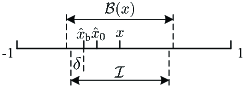
We first construct a time-invariant set ℐ ℐ \mathcal{I} x 𝑥 x x ∈ ℐ ⊂ ℬ ( x ) 𝑥 ℐ ℬ 𝑥 x\in\mathcal{I}\subset\mathcal{B}(x) δ 𝛿 \delta
inf v ∈ ∂ ℬ ( x ) , t ≥ 0 | v − x ~ 0 ( t ) | = inf v ∈ ∂ ℬ ( x ) | v − x ^ b | > δ > 0 , subscript infimum formulae-sequence 𝑣 ℬ 𝑥 𝑡 0 𝑣 superscript ~ 𝑥 0 𝑡 subscript infimum 𝑣 ℬ 𝑥 𝑣 subscript ^ 𝑥 b 𝛿 0 \inf_{v\in\partial\mathcal{B}(x),t\geq 0}\left|v-\tilde{x}^{0}(t)\right|=\inf_{v\in\partial\mathcal{B}(x)}\left|v-\hat{x}_{\text{b}}\right|>\delta>0, (51)
where x ^ b = x ~ 0 ( t b ) subscript ^ 𝑥 b superscript ~ 𝑥 0 subscript 𝑡 b \hat{x}_{\text{b}}=\tilde{x}^{0}(t_{\text{b}}) 𝝍 ~ 0 ( t ) superscript ~ 𝝍 0 𝑡 \tilde{\boldsymbol{\psi}}^{0}(t) 7 t ≥ t b 𝑡 subscript 𝑡 𝑏 t\geq t_{b} 𝝍 ~ 0 ( t ) superscript ~ 𝝍 0 𝑡 \tilde{\boldsymbol{\psi}}^{0}(t) 49 β 𝛽 \beta x 𝑥 x t 𝑡 t ℐ ℐ \mathcal{I}
ℐ = ( x − | x − x ^ b | − δ , x + | x − x ^ b | + δ ) ⊂ ℬ ( x ) . ℐ 𝑥 𝑥 subscript ^ 𝑥 b 𝛿 𝑥 𝑥 subscript ^ 𝑥 b 𝛿 ℬ 𝑥 \displaystyle\mathcal{I}=\Big{(}x-|x-\hat{x}_{\text{b}}|-\delta,~{}x+|x-\hat{x}_{\text{b}}|+\delta\Big{)}\subset\mathcal{B}(x). (52)
An example of the invariant set ℐ ℐ \mathcal{I} 7
Figure 7: An illustration of the invariant set ℐ ℐ \mathcal{I}
Then, we will establish a sufficient condition in Lemma 1 x ^ n ∈ ℐ for n ≥ 0 subscript ^ 𝑥 𝑛 ℐ for 𝑛 0 \hat{x}_{n}\!\in\!\mathcal{I}~{}\text{for}~{}n\!\geq\!0 [22 ] , we can obtain that { x ^ n } subscript ^ 𝑥 𝑛 \{\hat{x}_{n}\} x 𝑥 x 1
•
Pick T > 0 𝑇 0 T>0 𝝍 ~ 0 ( t ) , t ≥ 0 superscript ~ 𝝍 0 𝑡 𝑡
0 \tilde{\boldsymbol{\psi}}^{0}(t),t\geq 0 49 𝝍 ~ 0 ( 0 ) = [ β ^ 0 re , β ^ 0 im , x ^ 0 ] T superscript ~ 𝝍 0 0 superscript subscript superscript ^ 𝛽 re 0 subscript superscript ^ 𝛽 im 0 subscript ^ 𝑥 0
T \tilde{\boldsymbol{\psi}}^{0}(0)\!=\![\hat{\beta}^{\text{re}}_{0},\hat{\beta}^{\text{im}}_{0},\hat{x}_{0}]^{\text{T}} inf v ∈ ∂ ℬ | v − x ~ 0 ( t ) | ≥ 2 δ subscript infimum 𝑣 ℬ 𝑣 superscript ~ 𝑥 0 𝑡 2 𝛿 \inf_{v\in\partial\mathcal{B}}\left|v\!-\!\tilde{x}^{0}(t)\right|\geq 2\delta t ≥ T 𝑡 𝑇 t\geq T t ≥ t b 𝑡 subscript 𝑡 𝑏 t\geq t_{b} x ~ 0 ( t ) superscript ~ 𝑥 0 𝑡 \tilde{x}^{0}(t) x 𝑥 x t 𝑡 t T 𝑇 T
T = arg min t ∈ [ t b , ∞ ] | | [ ∫ t b t 𝐟 ( 𝝍 ~ 0 ( v ) , 𝝍 ) 𝑑 v ] 3 | − δ | , 𝑇 subscript 𝑡 subscript 𝑡 b subscript delimited-[] superscript subscript subscript 𝑡 b 𝑡 𝐟 superscript ~ 𝝍 0 𝑣 𝝍 differential-d 𝑣 3 𝛿 \displaystyle T=\arg\min\limits_{t\in[t_{\text{b}},\infty]}\left|~{}\!\!\left|\!\left[\int_{t_{\text{b}}}^{t}\mathbf{f}\left(\tilde{\boldsymbol{\psi}}^{0}(v),\boldsymbol{\psi}\right)dv\right]_{3}\right|-\delta\right|, (53)
where [ ⋅ ] i subscript delimited-[] ⋅ 𝑖 [\cdot]_{i} i 𝑖 i
•
Let T 0 = Δ 0 subscript 𝑇 0 Δ 0 T_{0}\overset{\Delta}{=}0 T m + 1 = Δ min { t i : t i ≥ T n + T , i ≥ 0 } subscript 𝑇 𝑚 1 Δ : subscript 𝑡 𝑖 formulae-sequence subscript 𝑡 𝑖 subscript 𝑇 𝑛 𝑇 𝑖 0 T_{m+1}\overset{\Delta}{=}\min\left\{t_{i}:t_{i}\geq T_{n}+T,i\geq 0\right\} m ≥ 0 𝑚 0 m\geq 0 T m + 1 − T m ∈ [ T , T + a 1 ] subscript 𝑇 𝑚 1 subscript 𝑇 𝑚 𝑇 𝑇 subscript 𝑎 1 T_{m+1}-T_{m}\in[T,T+a_{1}] T m = t n ~ ( m ) subscript 𝑇 𝑚 subscript 𝑡 ~ 𝑛 𝑚 T_{m}=t_{\tilde{n}(m)} n ~ ( m ) ↑ ∞ ↑ ~ 𝑛 𝑚 \tilde{n}(m)\uparrow\infty n ~ ( 0 ) = 0 ~ 𝑛 0 0 \tilde{n}(0)=0 𝝍 ~ n ~ ( m ) ( t ) superscript ~ 𝝍 ~ 𝑛 𝑚 𝑡 \tilde{\boldsymbol{\psi}}^{\tilde{n}(m)}(t) 49 t ∈ I m = Δ [ T m , T m + 1 ] 𝑡 subscript 𝐼 𝑚 Δ subscript 𝑇 𝑚 subscript 𝑇 𝑚 1 t\in I_{m}\overset{\Delta}{=}\left[T_{m},T_{m+1}\right] 𝝍 ~ n ~ ( m ) ( T m ) = 𝝍 ¯ ( T m ) superscript ~ 𝝍 ~ 𝑛 𝑚 subscript 𝑇 𝑚 ¯ 𝝍 subscript 𝑇 𝑚 \tilde{\boldsymbol{\psi}}^{\tilde{n}(m)}(T_{m})=\bar{\boldsymbol{\psi}}(T_{m}) m ≥ 0 𝑚 0 m\geq 0
Hence, we can obtain the following lemma:
Lemma 1 .
If sup t ∈ I m | x ¯ ( t ) − x ~ n ~ ( m ) ( t ) | ≤ δ 𝑡 subscript 𝐼 𝑚 supremum ¯ 𝑥 𝑡 superscript ~ 𝑥 ~ 𝑛 𝑚 𝑡 𝛿 \underset{t\in I_{m}}{\sup}\left|\bar{x}(t)-\tilde{x}^{\tilde{n}(m)}(t)\right|\leq\delta m ≥ 0 𝑚 0 m\geq 0 x ^ n ∈ ℐ for all n ≥ 0 subscript ^ 𝑥 𝑛 ℐ for all 𝑛 0 \hat{x}_{n}\in\mathcal{I}~{}\text{for all}~{}n\geq 0
Step 3: We will derive the probability lower bound for the condition in Lemma 1 P ( x ^ n → x | x ^ 0 ∈ ℬ ( x ) ) 𝑃 → subscript ^ 𝑥 𝑛 conditional 𝑥 subscript ^ 𝑥 0 ℬ 𝑥 P\left(\left.\hat{x}_{n}\!\rightarrow\!x\right|\hat{x}_{0}\!\in\!\mathcal{B}\left(x\right)\right)
We will derive the probability lower bound for the condition in Lemma 1
Lemma 2 .
If (i) the initial point satisfies x ^ 0 ∈ ℬ ( x ) subscript ^ 𝑥 0 ℬ 𝑥 \hat{x}_{0}\in\mathcal{B}(x) a n subscript 𝑎 𝑛 a_{n} 26 α > 0 𝛼 0 \alpha>0 N 0 ≥ 0 subscript 𝑁 0 0 N_{0}\geq 0 C > 0 𝐶 0 C>0
P ( x ^ n ∈ ℐ , ∀ n ≥ 0 ) ≥ 1 − 6 e − C | s | 2 α 2 σ 0 2 . 𝑃 formulae-sequence subscript ^ 𝑥 𝑛 ℐ for-all 𝑛 0 1 6 superscript 𝑒 𝐶 superscript 𝑠 2 superscript 𝛼 2 superscript subscript 𝜎 0 2 \displaystyle P\left(\hat{x}_{n}\in\mathcal{I},\forall n\geq 0\right)\geq 1-6e^{-\frac{C|s|^{2}}{\alpha^{2}\sigma_{0}^{2}}}. (54)
Finally, by applying Lemma 2 [22 ] , we can obtain
P ( x ^ n → x | x ^ 0 ∈ ℬ ) ≥ 𝑃 → subscript ^ 𝑥 𝑛 conditional 𝑥 subscript ^ 𝑥 0 ℬ absent \displaystyle P\left(\left.\hat{x}_{n}\rightarrow x\right|\hat{x}_{0}\in\mathcal{B}\right)\geq P ( x ^ n ∈ ℐ , ∀ n ≥ 0 ) 𝑃 formulae-sequence subscript ^ 𝑥 𝑛 ℐ for-all 𝑛 0 \displaystyle~{}P\left(\hat{x}_{n}\in\mathcal{I},\forall n\geq 0\right) (55)
≥ \displaystyle\geq 1 − 6 e − C | s | 2 α 2 σ 0 2 , 1 6 superscript 𝑒 𝐶 superscript 𝑠 2 superscript 𝛼 2 superscript subscript 𝜎 0 2 \displaystyle~{}1-6e^{-\frac{C|{s}|^{2}}{\alpha^{2}\sigma_{0}^{2}}},
which completes the proof of Theorem 2
Appendix C Proof of Theorem 3
When the step-size a n subscript 𝑎 𝑛 a_{n} 26 α > 0 𝛼 0 \alpha>0 N 0 ≥ 0 subscript 𝑁 0 0 N_{0}\geq 0 [19 , Section 6.6] has proposed the sufficient conditions to prove the asymptotic normality of n ( x ^ n − x ) 𝑛 subscript ^ 𝑥 𝑛 𝑥 \sqrt{n}\left(\hat{x}_{n}-x\right) n ( x ^ n − x ) → 𝑑 𝒩 ( 0 , Σ x ) 𝑛 subscript ^ 𝑥 𝑛 𝑥 𝑑 → 𝒩 0 subscript Σ 𝑥 \sqrt{n}\left(\hat{x}_{n}-x\right)\overset{d}{\rightarrow}\mathcal{N}\left(0,\Sigma_{x}\right) 𝝍 ^ n → 𝝍 → subscript ^ 𝝍 𝑛 𝝍 \hat{\boldsymbol{\psi}}_{n}\rightarrow\boldsymbol{\psi} Σ Σ \Sigma
1)
Equation (29 σ 𝜎 \sigma { ℱ n : n ≥ 0 } conditional-set subscript ℱ 𝑛 𝑛 0 \{\mathcal{F}_{n}:n\geq 0\} ℱ m ⊂ ℱ n subscript ℱ 𝑚 subscript ℱ 𝑛 \mathcal{F}_{m}\!\subset\!\mathcal{F}_{n} m < n 𝑚 𝑛 m\!<\!n 𝐳 ^ n subscript ^ 𝐳 𝑛 \hat{\mathbf{z}}_{n} ℱ n subscript ℱ 𝑛 \mathcal{F}_{n} ℱ n − 1 subscript ℱ 𝑛 1 \mathcal{F}_{n-1} A σ 𝜎 \sigma { 𝒢 n : n ≥ 0 } conditional-set subscript 𝒢 𝑛 𝑛 0 \{\mathcal{G}_{n}:n\geq 0\} 𝐳 ^ n subscript ^ 𝐳 𝑛 \hat{\mathbf{z}}_{n} 𝒢 n subscript 𝒢 𝑛 \mathcal{G}_{n} 𝔼 [ 𝐳 ^ n | 𝒢 n ] = 𝐳 ^ n 𝔼 delimited-[] conditional subscript ^ 𝐳 𝑛 subscript 𝒢 𝑛 subscript ^ 𝐳 𝑛 \mathbb{E}\left[\left.\hat{\mathbf{z}}_{n}\right|\mathcal{G}_{n}\right]=\hat{\mathbf{z}}_{n} 𝒢 n − 1 subscript 𝒢 𝑛 1 \mathcal{G}_{n-1} 𝔼 [ 𝐳 ^ n | 𝒢 n − 1 ] = 𝔼 [ 𝐳 ^ n ] = 𝟎 𝔼 delimited-[] conditional subscript ^ 𝐳 𝑛 subscript 𝒢 𝑛 1 𝔼 delimited-[] subscript ^ 𝐳 𝑛 0 \mathbb{E}\left[\left.\hat{\mathbf{z}}_{n}\right|\mathcal{G}_{n-1}\right]=\mathbb{E}\left[\hat{\mathbf{z}}_{n}\right]=\mathbf{0}
2)
x ^ n subscript ^ 𝑥 𝑛 \hat{x}_{n} x 𝑥 x n → ∞ → 𝑛 n\rightarrow\infty 𝝍 ^ n → 𝝍 → subscript ^ 𝝍 𝑛 𝝍 \hat{\boldsymbol{\psi}}_{n}\rightarrow\boldsymbol{\psi} x ^ n subscript ^ 𝑥 𝑛 \hat{x}_{n} x 𝑥 x n → ∞ → 𝑛 n\rightarrow\infty
3)
The stable condition:
20 𝐟 ( 𝝍 ^ n − 1 , 𝝍 ) 𝐟 subscript ^ 𝝍 𝑛 1 𝝍 \mathbf{f}\left(\hat{\boldsymbol{\psi}}_{n-1},\boldsymbol{\psi}\right)
𝐟 ( 𝝍 ^ n − 1 , 𝝍 ) = 𝐂 1 ( 𝝍 ^ n − 1 − 𝝍 ) + [ o ( ‖ 𝝍 ^ n − 1 − 𝝍 ‖ 2 ) o ( ‖ 𝝍 ^ n − 1 − 𝝍 ‖ 2 ) o ( ‖ 𝝍 ^ n − 1 − 𝝍 ‖ 2 ) ] , 𝐟 subscript ^ 𝝍 𝑛 1 𝝍 subscript 𝐂 1 subscript ^ 𝝍 𝑛 1 𝝍 delimited-[] matrix 𝑜 subscript norm subscript ^ 𝝍 𝑛 1 𝝍 2 𝑜 subscript norm subscript ^ 𝝍 𝑛 1 𝝍 2 𝑜 subscript norm subscript ^ 𝝍 𝑛 1 𝝍 2 \displaystyle\!\!\!\!\!\!\mathbf{f}\left(\hat{\boldsymbol{\psi}}_{n-1},\boldsymbol{\psi}\right)\!=\!\mathbf{C}_{1}\left(\hat{\boldsymbol{\psi}}_{n-1}-\boldsymbol{\psi}\right)\!+\!\left[\begin{matrix}o(\|\hat{\boldsymbol{\psi}}_{n-1}-\boldsymbol{\psi}\|_{2})\\
o(\|\hat{\boldsymbol{\psi}}_{n-1}-\boldsymbol{\psi}\|_{2})\\
o(\|\hat{\boldsymbol{\psi}}_{n-1}-\boldsymbol{\psi}\|_{2})\end{matrix}\right]\!\!, (56)
where 𝐂 1 subscript 𝐂 1 \mathbf{C}_{1}
𝐂 1 = ∂ 𝐟 ( 𝝍 ^ n − 1 , 𝝍 ) ∂ 𝝍 ^ n − 1 T | 𝝍 ^ n − 1 = 𝝍 = − [ 1 0 0 0 1 0 0 0 1 ] . subscript 𝐂 1 evaluated-at 𝐟 subscript ^ 𝝍 𝑛 1 𝝍 superscript subscript ^ 𝝍 𝑛 1 T subscript ^ 𝝍 𝑛 1 𝝍 delimited-[] matrix 1 0 0 0 1 0 0 0 1 \displaystyle\mathbf{C}_{1}=\left.\frac{\partial\mathbf{f}\left(\hat{\boldsymbol{\psi}}_{n-1},\boldsymbol{\psi}\right)}{\partial\hat{\boldsymbol{\psi}}_{n-1}^{\text{T}}}\right|_{\hat{\boldsymbol{\psi}}_{n-1}=\boldsymbol{\psi}}=-\left[\begin{matrix}1&0&0\\
0&1&0\\
0&0&1\end{matrix}\right]. (57)
Then we get the stable condition that
𝐀 = 𝐂 1 ⋅ α + 1 2 = − [ α − 1 2 0 0 0 α − 1 2 0 0 0 α − 1 2 ] ≺ 0 , 𝐀 ⋅ subscript 𝐂 1 𝛼 1 2 delimited-[] matrix 𝛼 1 2 0 0 0 𝛼 1 2 0 0 0 𝛼 1 2 precedes 0 \displaystyle\mathbf{A}\!=\!\mathbf{C}_{1}\cdot\alpha+\frac{1}{2}\!=\!-\!\left[\begin{matrix}\alpha\!-\!\frac{1}{2}&0&0\\
0&\alpha\!-\!\frac{1}{2}&0\\
0&0&\alpha\!-\!\frac{1}{2}\end{matrix}\right]\prec 0, (58)
which results in α > 1 2 𝛼 1 2 \alpha>\frac{1}{2}
4)
The constraints for the noise vector 𝐳 ^ n subscript ^ 𝐳 𝑛 \hat{\mathbf{z}}_{n}
𝔼 [ ‖ 𝐳 ^ n ‖ 2 2 ] = tr ( 𝐈 ( 𝝍 ^ n − 1 , 𝐖 n ) − 1 ) < ∞ , 𝔼 delimited-[] superscript subscript norm subscript ^ 𝐳 𝑛 2 2 tr 𝐈 superscript subscript ^ 𝝍 𝑛 1 subscript 𝐖 𝑛 1 \mathbb{E}\left[\left\|\hat{\mathbf{z}}_{n}\right\|_{2}^{2}\right]=\operatorname{tr}(\mathbf{I}(\hat{\boldsymbol{\psi}}_{n\!-\!1},\!\mathbf{W}_{n})^{-1})<\infty, (59)
and
lim v → ∞ sup n ≥ 1 ∫ ‖ z ^ n ‖ 2 > v ‖ 𝐳 ^ n ‖ 2 2 p ( 𝐳 ^ n ) 𝑑 𝐳 ^ n = 0 . → 𝑣 𝑛 1 supremum subscript subscript norm subscript ^ 𝑧 𝑛 2 𝑣 superscript subscript norm subscript ^ 𝐳 𝑛 2 2 𝑝 subscript ^ 𝐳 𝑛 differential-d subscript ^ 𝐳 𝑛
0 \underset{v\rightarrow\infty}{\lim}\ \ \underset{n\geq 1}{\sup}\ \ \int\limits_{\left\|\hat{z}_{n}\right\|_{2}>v}\left\|\hat{\mathbf{z}}_{n}\right\|_{2}^{2}p(\hat{\mathbf{z}}_{n})d\hat{\mathbf{z}}_{n}=0. (60)
Let
𝐁 = 𝐁 absent \displaystyle\mathbf{B}= lim n → ∞ 𝝍 ^ n → 𝝍 𝔼 [ 𝐳 ^ n 𝐳 ^ n T ] subscript matrix → 𝑛 → subscript ^ 𝝍 𝑛 𝝍 𝔼 delimited-[] subscript ^ 𝐳 𝑛 superscript subscript ^ 𝐳 𝑛 T \displaystyle~{}\lim_{\begin{matrix}n\rightarrow\infty\\
\hat{\boldsymbol{\psi}}_{n}\rightarrow\boldsymbol{\psi}\end{matrix}}\mathbb{E}\left[\hat{\mathbf{z}}_{n}\hat{\mathbf{z}}_{n}^{\text{T}}\right] (61)
= ( a ) 𝑎 \displaystyle\overset{(a)}{=} lim n → ∞ 𝝍 ^ n → 𝝍 𝐈 ( 𝝍 ^ n , 𝐖 n + 1 ) − 1 = 𝐈 ( 𝝍 , 𝐖 ∗ ) − 1 , subscript matrix → 𝑛 → subscript ^ 𝝍 𝑛 𝝍 𝐈 superscript subscript ^ 𝝍 𝑛 subscript 𝐖 𝑛 1 1 𝐈 superscript 𝝍 superscript 𝐖 1 \displaystyle~{}\lim_{\begin{matrix}n\rightarrow\infty\\
\hat{\boldsymbol{\psi}}_{n}\rightarrow\boldsymbol{\psi}\end{matrix}}\mathbf{I}(\hat{\boldsymbol{\psi}}_{n},\!\mathbf{W}_{n\!+\!1})^{-1}=\mathbf{I}(\boldsymbol{\psi},\mathbf{W}^{*})^{-1},
where step ( a ) 𝑎 (a) 31
Then, from Theorem 6.6.1 [19 , Section 6.6] , we have
n + N 0 ( 𝝍 ^ n − 𝝍 ) → 𝑑 𝒩 ( 0 , 𝚺 ) , 𝑛 subscript 𝑁 0 subscript ^ 𝝍 𝑛 𝝍 𝑑 → 𝒩 0 𝚺 \displaystyle\sqrt{n+N_{0}}\left(\hat{\boldsymbol{\psi}}_{n}-\boldsymbol{\psi}\right)\overset{d}{\rightarrow}\mathcal{N}\left(0,\boldsymbol{\Sigma}\right),
where
𝚺 = 𝚺 absent \displaystyle\boldsymbol{\Sigma}= α 2 ⋅ ∫ 0 ∞ e 𝐀 v 𝐁 e 𝐀 H v 𝑑 v ⋅ superscript 𝛼 2 superscript subscript 0 superscript 𝑒 𝐀 𝑣 𝐁 superscript 𝑒 superscript 𝐀 H 𝑣 differential-d 𝑣 \displaystyle~{}\alpha^{2}\cdot\int_{0}^{\infty}e^{\mathbf{A}v}\mathbf{B}e^{\mathbf{A}^{\text{H}}v}dv (62)
= \displaystyle= α 2 2 α − 1 𝐈 ( 𝝍 , 𝐖 ∗ ) − 1 . superscript 𝛼 2 2 𝛼 1 𝐈 superscript 𝝍 superscript 𝐖 1 \displaystyle~{}\frac{\alpha^{2}}{2\alpha-1}\mathbf{I}(\boldsymbol{\psi},\mathbf{W}^{*})^{-1}.
Due to that lim n → ∞ ( n + N 0 ) / n = 1 subscript → 𝑛 𝑛 subscript 𝑁 0 𝑛 1 \lim_{n\rightarrow\infty}\sqrt{{(n+N_{0})}/{n}}=1
n ( 𝝍 ^ n − 𝝍 ) → n ⋅ n + N 0 n ( 𝝍 ^ n − 𝝍 ) → 𝑑 𝒩 ( 0 , 𝚺 ) , → 𝑛 subscript ^ 𝝍 𝑛 𝝍 ⋅ 𝑛 𝑛 subscript 𝑁 0 𝑛 subscript ^ 𝝍 𝑛 𝝍 𝑑 → 𝒩 0 𝚺 \displaystyle\sqrt{n}\left(\hat{\boldsymbol{\psi}}_{n}-\boldsymbol{\psi}\right)\rightarrow\sqrt{n}\cdot\sqrt{\frac{n+N_{0}}{n}}\left(\hat{\boldsymbol{\psi}}_{n}-\boldsymbol{\psi}\right)\overset{d}{\rightarrow}\mathcal{N}\left(0,\boldsymbol{\Sigma}\right),
as n → ∞ → 𝑛 n\rightarrow\infty
n ( x ^ n − x ) → 𝑑 𝒩 ( 0 , [ 𝚺 ] 3 , 3 ) . 𝑛 subscript ^ 𝑥 𝑛 𝑥 𝑑 → 𝒩 0 subscript delimited-[] 𝚺 3 3
\displaystyle\sqrt{n}\left(\hat{x}_{n}-x\right)\overset{d}{\rightarrow}\mathcal{N}\left(0,\left[\boldsymbol{\Sigma}\right]_{3,3}\right). (63)
By adapting α 𝛼 \alpha 62 [ 𝚺 ] 3 , 3 subscript delimited-[] 𝚺 3 3
\left[\boldsymbol{\Sigma}\right]_{3,3} [ 𝐈 ( 𝝍 , 𝐖 ∗ ) − 1 ] 3 , 3 subscript delimited-[] 𝐈 superscript 𝝍 superscript 𝐖 1 3 3
\left[\mathbf{I}(\boldsymbol{\psi},\mathbf{W}^{*})^{-1}\right]_{3,3} III-A α = 1 𝛼 1 \alpha=1
By assuming α = 1 𝛼 1 \alpha=1
lim n → ∞ n 𝔼 [ ( x ^ n − x ) 2 | 𝝍 ^ n → 𝝍 ] = [ 𝐈 ( 𝝍 , 𝐖 ∗ ) − 1 ] 3 , 3 . subscript → 𝑛 𝑛 𝔼 delimited-[] → conditional superscript subscript ^ 𝑥 𝑛 𝑥 2 subscript ^ 𝝍 𝑛 𝝍 subscript delimited-[] 𝐈 superscript 𝝍 superscript 𝐖 1 3 3
\lim_{n\rightarrow\infty}~{}n~{}\mathbb{E}\left[\left(\hat{x}_{n}-x\right)^{2}\big{|}\hat{\boldsymbol{\psi}}_{n}\rightarrow\boldsymbol{\psi}\right]=\left[\mathbf{I}(\boldsymbol{\psi},\mathbf{W}^{*})^{-1}\right]_{3,3}.
Appendix D Proof of Lemma 1
When m = 0 𝑚 0 m=0 x ~ n ~ ( 0 ) ( T 0 ) = x ¯ ( T 0 ) = x ^ 0 superscript ~ 𝑥 ~ 𝑛 0 subscript 𝑇 0 ¯ 𝑥 subscript 𝑇 0 subscript ^ 𝑥 0 \tilde{x}^{\tilde{n}(0)}(T_{0})=\bar{x}(T_{0})=\hat{x}_{0} x ^ 0 < x subscript ^ 𝑥 0 𝑥 \hat{x}_{0}<x x ^ 0 > x subscript ^ 𝑥 0 𝑥 \hat{x}_{0}>x
Case 1 (x ^ 0 < x subscript ^ 𝑥 0 𝑥 \hat{x}_{0}<x x ¯ ( t ) ∈ ℐ = ( x − | x − x ^ b | − δ , x + | x − x ^ b | + δ ) ¯ 𝑥 𝑡 ℐ 𝑥 𝑥 subscript ^ 𝑥 𝑏 𝛿 𝑥 𝑥 subscript ^ 𝑥 𝑏 𝛿 \bar{x}(t)\in\mathcal{I}=\Big{(}x-|x-\hat{x}_{b}|-\delta,~{}x+|x-\hat{x}_{b}|+\delta\Big{)} t ∈ I 0 𝑡 subscript 𝐼 0 t\in I_{0}
If | x ¯ ( t ) − x ~ n ~ ( 0 ) ( t ) | ≤ δ ¯ 𝑥 𝑡 superscript ~ 𝑥 ~ 𝑛 0 𝑡 𝛿 \left|\bar{x}(t)-\tilde{x}^{\tilde{n}(0)}(t)\right|\leq\delta t ∈ I 0 𝑡 subscript 𝐼 0 t\in I_{0}
− δ ≤ x ¯ ( t ) − x ~ n ~ ( 0 ) ( t ) ≤ δ . 𝛿 ¯ 𝑥 𝑡 superscript ~ 𝑥 ~ 𝑛 0 𝑡 𝛿 -\delta\leq\bar{x}(t)-\tilde{x}^{\tilde{n}(0)}(t)\leq\delta. (64)
What’s more, due to the definition of x ^ b subscript ^ 𝑥 b \hat{x}_{\text{b}} 51
x ^ b ≤ x , x ~ n ~ ( 0 ) ( t ) − x ^ b ≥ 0 , x − x ~ n ~ ( 0 ) ( t ) ≥ 0 , formulae-sequence subscript ^ 𝑥 b 𝑥 formulae-sequence superscript ~ 𝑥 ~ 𝑛 0 𝑡 subscript ^ 𝑥 b 0 𝑥 superscript ~ 𝑥 ~ 𝑛 0 𝑡 0 \hat{x}_{\text{b}}\leq x,\tilde{x}^{\tilde{n}(0)}(t)-\hat{x}_{\text{b}}\geq 0,x-\tilde{x}^{\tilde{n}(0)}(t)\geq 0, (65)
for all t ∈ I 0 𝑡 subscript 𝐼 0 t\in I_{0} 64 65
x ¯ ( t ) − ( x − | x − x ^ b | − δ ) ¯ 𝑥 𝑡 𝑥 𝑥 subscript ^ 𝑥 𝑏 𝛿 \displaystyle~{}\bar{x}(t)-(x-|x-\hat{x}_{b}|-\delta) (66)
= \displaystyle= x ¯ ( t ) − ( x ^ b − δ ) ¯ 𝑥 𝑡 subscript ^ 𝑥 b 𝛿 \displaystyle~{}\bar{x}(t)-(\hat{x}_{\text{b}}-\delta)
= \displaystyle= [ x ¯ ( t ) − x ~ n ~ ( 0 ) ( t ) ] + [ x ~ n ~ ( 0 ) ( t ) − x ^ b ] + δ ≥ 0 , delimited-[] ¯ 𝑥 𝑡 superscript ~ 𝑥 ~ 𝑛 0 𝑡 delimited-[] superscript ~ 𝑥 ~ 𝑛 0 𝑡 subscript ^ 𝑥 b 𝛿 0 \displaystyle~{}\left[\bar{x}(t)-\tilde{x}^{\tilde{n}(0)}(t)\right]+\left[\tilde{x}^{\tilde{n}(0)}(t)-\hat{x}_{\text{b}}\right]+\delta\geq 0,
and
( x + | x − x ^ b | + δ ) − x ¯ ( t ) 𝑥 𝑥 subscript ^ 𝑥 b 𝛿 ¯ 𝑥 𝑡 \displaystyle~{}(x+|x-\hat{x}_{\text{b}}|+\delta)-\bar{x}(t) (67)
= \displaystyle= ( 2 x − x ^ b + δ ) − x ¯ ( t ) 2 𝑥 subscript ^ 𝑥 b 𝛿 ¯ 𝑥 𝑡 \displaystyle~{}(2x-\hat{x}_{\text{b}}+\delta)-\bar{x}(t)
= \displaystyle= ( x − x ^ b ) + [ x − x ¯ ( t ) ] + δ 𝑥 subscript ^ 𝑥 b delimited-[] 𝑥 ¯ 𝑥 𝑡 𝛿 \displaystyle~{}\left(x-\hat{x}_{\text{b}}\right)+\left[x-\bar{x}(t)\right]+\delta
= \displaystyle= ( x − x ^ b ) + [ x − x ~ n ~ ( 0 ) ( t ) ] + [ x ~ n ~ ( 0 ) ( t ) − x ¯ ( t ) ] + δ 𝑥 subscript ^ 𝑥 b delimited-[] 𝑥 superscript ~ 𝑥 ~ 𝑛 0 𝑡 delimited-[] superscript ~ 𝑥 ~ 𝑛 0 𝑡 ¯ 𝑥 𝑡 𝛿 \displaystyle~{}\left(x-\hat{x}_{\text{b}}\right)+\left[x-\tilde{x}^{\tilde{n}(0)}(t)\right]+\left[\tilde{x}^{\tilde{n}(0)}(t)-\bar{x}(t)\right]+\delta
≥ \displaystyle\geq 0 , 0 \displaystyle~{}0,
which result in x ¯ ( t ) ∈ ℐ ¯ 𝑥 𝑡 ℐ \bar{x}(t)\in\mathcal{I} t ∈ I 0 𝑡 subscript 𝐼 0 t\in I_{0}
Then, we consider the initial value x ¯ ( T 1 ) ¯ 𝑥 subscript 𝑇 1 \bar{x}(T_{1}) I 1 subscript 𝐼 1 I_{1} T 𝑇 T 53
x − x ^ b ≥ x ~ n ~ ( 0 ) ( T 1 ) − x ^ b ≥ x ~ n ~ ( 0 ) ( T ) − x ^ b ≥ δ . 𝑥 subscript ^ 𝑥 b superscript ~ 𝑥 ~ 𝑛 0 subscript 𝑇 1 subscript ^ 𝑥 b superscript ~ 𝑥 ~ 𝑛 0 𝑇 subscript ^ 𝑥 b 𝛿 \displaystyle x-\hat{x}_{\text{b}}\geq\tilde{x}^{\tilde{n}(0)}(T_{1})-\hat{x}_{\text{b}}\geq\tilde{x}^{\tilde{n}(0)}(T)-\hat{x}_{\text{b}}\geq\delta. (68)
By using (64 65 68
x ¯ ( T 1 ) − ( x − | x − x ^ b | ) ¯ 𝑥 subscript 𝑇 1 𝑥 𝑥 subscript ^ 𝑥 b \displaystyle~{}\bar{x}(T_{1})-(x-|x-\hat{x}_{\text{b}}|) (69)
= \displaystyle= x ¯ ( T 1 ) − x ^ b ¯ 𝑥 subscript 𝑇 1 subscript ^ 𝑥 b \displaystyle~{}\bar{x}(T_{1})-\hat{x}_{\text{b}}
= \displaystyle= [ x ¯ ( T 1 ) − x ~ n ~ ( 0 ) ( T 1 ) ] + [ x ~ n ~ ( 0 ) ( T 1 ) − x ^ b ] ≥ 0 , delimited-[] ¯ 𝑥 subscript 𝑇 1 superscript ~ 𝑥 ~ 𝑛 0 subscript 𝑇 1 delimited-[] superscript ~ 𝑥 ~ 𝑛 0 subscript 𝑇 1 subscript ^ 𝑥 b 0 \displaystyle~{}\left[\bar{x}(T_{1})-\tilde{x}^{\tilde{n}(0)}(T_{1})\right]+\left[\tilde{x}^{\tilde{n}(0)}(T_{1})-\hat{x}_{\text{b}}\right]\geq 0,
and
( x + | x − x ^ b | ) − x ¯ ( T 1 ) 𝑥 𝑥 subscript ^ 𝑥 b ¯ 𝑥 subscript 𝑇 1 \displaystyle~{}(x+|x-\hat{x}_{\text{b}}|)-\bar{x}(T_{1}) (70)
= \displaystyle= ( 2 x − x ^ b ) − x ¯ ( T 1 ) 2 𝑥 subscript ^ 𝑥 b ¯ 𝑥 subscript 𝑇 1 \displaystyle~{}(2x-\hat{x}_{\text{b}})-\bar{x}(T_{1})
= \displaystyle= ( x − x ^ b ) + [ x − x ¯ ( T 1 ) ] 𝑥 subscript ^ 𝑥 b delimited-[] 𝑥 ¯ 𝑥 subscript 𝑇 1 \displaystyle~{}\left(x-\hat{x}_{\text{b}}\right)+\left[x-\bar{x}(T_{1})\right]
= \displaystyle= ( x − x ^ b ) + [ x − x ~ n ~ ( 0 ) ( T 1 ) ] + [ x ~ n ~ ( 0 ) ( T 1 ) − x ¯ ( T 1 ) ] 𝑥 subscript ^ 𝑥 b delimited-[] 𝑥 superscript ~ 𝑥 ~ 𝑛 0 subscript 𝑇 1 delimited-[] superscript ~ 𝑥 ~ 𝑛 0 subscript 𝑇 1 ¯ 𝑥 subscript 𝑇 1 \displaystyle~{}\left(x-\hat{x}_{\text{b}}\right)+\left[x-\tilde{x}^{\tilde{n}(0)}(T_{1})\right]+\left[\tilde{x}^{\tilde{n}(0)}(T_{1})-\bar{x}(T_{1})\right]
≥ \displaystyle\geq 0 , 0 \displaystyle~{}0,
which result in x ¯ ( T 1 ) ∈ [ x − | x − x ^ b | , x + | x − x ^ b | ] ¯ 𝑥 subscript 𝑇 1 𝑥 𝑥 subscript ^ 𝑥 b 𝑥 𝑥 subscript ^ 𝑥 b \bar{x}(T_{1})\in\big{[}x-|x-\hat{x}_{\text{b}}|,~{}x+|x-\hat{x}_{\text{b}}|\big{]}
Case 2 (x ^ 0 > x subscript ^ 𝑥 0 𝑥 \hat{x}_{0}>x 66 67 69 70 x ¯ ( t ) ∈ ℐ ¯ 𝑥 𝑡 ℐ \bar{x}(t)\in\mathcal{I} t ∈ I 0 𝑡 subscript 𝐼 0 t\in I_{0} x ¯ ( T 1 ) ∈ [ x − | x − x ^ b | , x + | x − x ^ b | ] ¯ 𝑥 subscript 𝑇 1 𝑥 𝑥 subscript ^ 𝑥 b 𝑥 𝑥 subscript ^ 𝑥 b \bar{x}(T_{1})\in\big{[}x-|x-\hat{x}_{\text{b}}|,~{}x+|x-\hat{x}_{\text{b}}|\big{]}
When m = 1 𝑚 1 m=1 x ~ n ~ ( 1 ) ( T 1 ) = x ¯ ( T 1 ) ∈ [ x − | x − x ^ b | , x + | x − x ^ b | ] superscript ~ 𝑥 ~ 𝑛 1 subscript 𝑇 1 ¯ 𝑥 subscript 𝑇 1 𝑥 𝑥 subscript ^ 𝑥 b 𝑥 𝑥 subscript ^ 𝑥 b \tilde{x}^{\tilde{n}(1)}(T_{1})=\bar{x}(T_{1})\in\big{[}x-|x-\hat{x}_{\text{b}}|,~{}x+|x-\hat{x}_{\text{b}}|\big{]} x ¯ ( T 1 ) < x ¯ 𝑥 subscript 𝑇 1 𝑥 \bar{x}(T_{1})<x | x ¯ ( t ) − x ~ n ~ ( 1 ) ( t ) | ≤ δ ¯ 𝑥 𝑡 superscript ~ 𝑥 ~ 𝑛 1 𝑡 𝛿 \left|\bar{x}(t)-\tilde{x}^{\tilde{n}(1)}(t)\right|\leq\delta t ∈ I 1 𝑡 subscript 𝐼 1 t\in I_{1} x ¯ ( T 1 ) ≥ x ^ b ¯ 𝑥 subscript 𝑇 1 subscript ^ 𝑥 b \bar{x}(T_{1})\geq\hat{x}_{\text{b}} x ~ n ~ ( 1 ) ( t ) − x ^ b ≥ 0 superscript ~ 𝑥 ~ 𝑛 1 𝑡 subscript ^ 𝑥 b 0 \tilde{x}^{\tilde{n}(1)}(t)-\hat{x}_{\text{b}}\geq 0 x − x ~ n ~ ( 1 ) ( t ) ≥ 0 𝑥 superscript ~ 𝑥 ~ 𝑛 1 𝑡 0 x-\tilde{x}^{\tilde{n}(1)}(t)\geq 0
x − x ^ b ≥ x ~ n ~ ( 1 ) ( T 2 ) − x ^ b ≥ x ~ n ~ ( 1 ) ( T 1 + T ) − x ^ b ≥ δ . 𝑥 subscript ^ 𝑥 b superscript ~ 𝑥 ~ 𝑛 1 subscript 𝑇 2 subscript ^ 𝑥 b superscript ~ 𝑥 ~ 𝑛 1 subscript 𝑇 1 𝑇 subscript ^ 𝑥 b 𝛿 \displaystyle x-\hat{x}_{\text{b}}\geq\tilde{x}^{\tilde{n}(1)}(T_{2})-\hat{x}_{\text{b}}\geq\tilde{x}^{\tilde{n}(1)}(T_{1}+T)-\hat{x}_{\text{b}}\geq\delta.
Similar to (66 67 69 70 x ¯ ( t ) ∈ ℐ for all t ∈ I 1 ¯ 𝑥 𝑡 ℐ for all 𝑡 subscript 𝐼 1 \bar{x}(t)\in\mathcal{I}~{}\text{for all}~{}t\in I_{1} x ¯ ( T 2 ) ∈ [ x − | x − x ^ b | , x + | x − x ^ b | ] ¯ 𝑥 subscript 𝑇 2 𝑥 𝑥 subscript ^ 𝑥 b 𝑥 𝑥 subscript ^ 𝑥 b \bar{x}(T_{2})\in\big{[}x-|x-\hat{x}_{\text{b}}|,~{}x+|x-\hat{x}_{\text{b}}|\big{]} x ¯ ( T 1 ) > x ¯ 𝑥 subscript 𝑇 1 𝑥 \bar{x}(T_{1})>x
Hence, we can use the same method to prove the cases of m ≥ 2 𝑚 2 m\geq 2 x ¯ ( t ) ∈ ℐ ¯ 𝑥 𝑡 ℐ \bar{x}(t)\in\mathcal{I} t ∈ I m 𝑡 subscript 𝐼 𝑚 t\in I_{m} m ≥ 0 𝑚 0 m\geq 0 x ¯ ( t n ) = x ^ n ¯ 𝑥 subscript 𝑡 𝑛 subscript ^ 𝑥 𝑛 \bar{x}(t_{n})=\hat{x}_{n} n ≥ 0 𝑛 0 n\geq 0 x ^ n ∈ ℐ for all n ≥ 0 subscript ^ 𝑥 𝑛 ℐ for all 𝑛 0 \hat{x}_{n}\in\mathcal{I}~{}\text{for all}~{}n\geq 0
Appendix E Proof of Lemma 2
The following lemmas are needed to prove Lemma 2
Lemma 3 .
Given T 𝑇 T 53
n T = Δ inf { i ∈ ℤ : t n + i ≥ t n + T } . subscript 𝑛 𝑇 Δ infimum conditional-set 𝑖 ℤ subscript 𝑡 𝑛 𝑖 subscript 𝑡 𝑛 𝑇 \displaystyle n_{T}\overset{\Delta}{=}\inf\left\{i\in\mathbb{Z}:t_{n+i}\geq t_{n}+T\right\}. (71)
If there exists a constant C > 0 𝐶 0 C>0
‖ 𝝍 ¯ ( t n + m ) − 𝝍 ~ n ( t n + m ) ‖ 2 subscript norm ¯ 𝝍 subscript 𝑡 𝑛 𝑚 superscript ~ 𝝍 𝑛 subscript 𝑡 𝑛 𝑚 2 \displaystyle~{}\left\|\bar{\boldsymbol{\psi}}(t_{n+m})-\tilde{\boldsymbol{\psi}}^{n}(t_{n+m})\right\|_{2} (72)
≤ \displaystyle\leq L ∑ i = 1 m a n + i ‖ 𝝍 ¯ ( t n + i − 1 ) − 𝝍 ~ n ( t n + i − 1 ) ‖ 2 + C , 𝐿 superscript subscript 𝑖 1 𝑚 subscript 𝑎 𝑛 𝑖 subscript norm ¯ 𝝍 subscript 𝑡 𝑛 𝑖 1 superscript ~ 𝝍 𝑛 subscript 𝑡 𝑛 𝑖 1 2 𝐶 \displaystyle~{}L\sum_{i=1}^{m}a_{n+i}\left\|\bar{\boldsymbol{\psi}}(t_{n+i-1})-\tilde{\boldsymbol{\psi}}^{n}(t_{n+i-1})\right\|_{2}+C,
for all n ≥ 0 𝑛 0 n\geq 0 1 ≤ m ≤ n T 1 𝑚 subscript 𝑛 𝑇 1\leq m\leq n_{T}
sup t ∈ [ t n , t n + n T ] ‖ 𝝍 ¯ ( t ) − 𝝍 ~ n ( t ) ‖ 2 ≤ C 𝐟 a n + 1 2 + C e L ( T + a 1 ) , 𝑡 subscript 𝑡 𝑛 subscript 𝑡 𝑛 subscript 𝑛 𝑇 supremum subscript norm ¯ 𝝍 𝑡 superscript ~ 𝝍 𝑛 𝑡 2 subscript 𝐶 𝐟 subscript 𝑎 𝑛 1 2 𝐶 superscript 𝑒 𝐿 𝑇 subscript 𝑎 1 \displaystyle\underset{t\in\left[t_{n},t_{n+n_{T}}\right]}{\sup}\left\|\bar{\boldsymbol{\psi}}(t)-\tilde{\boldsymbol{\psi}}^{n}(t)\right\|_{2}\leq\frac{C_{\mathbf{f}}a_{n+1}}{2}+Ce^{L(T+a_{1})}, (73)
where L 𝐿 L C 𝐟 subscript 𝐶 𝐟 C_{\mathbf{f}} 78 79
Lemma 4 (Lemma 4 [18 ] ).
If { M i : i = 1 , 2 , … } conditional-set subscript 𝑀 𝑖 𝑖 1 2 …
\{M_{i}:i=1,2,\ldots\} M i subscript 𝑀 𝑖 M_{i} M i subscript 𝑀 𝑖 M_{i} i 𝑖 i
P ( sup 0 ≤ i ≤ k | M i | > η ) ≤ 2 exp { − η 2 2 Var [ M k ] } , 𝑃 0 𝑖 𝑘 supremum subscript 𝑀 𝑖 𝜂 2 superscript 𝜂 2 2 Var subscript 𝑀 𝑘 \displaystyle P\left(\underset{0\leq i\leq k}{\sup}\left|M_{i}\right|>\eta\right)\leq 2\exp\left\{-\frac{\eta^{2}}{2\operatorname{Var}\left[M_{k}\right]}\right\}, (74)
for any η > 0 𝜂 0 \eta>0
Lemma 5 (Lemma 5 [18 ] ).
If given a constant C > 0 𝐶 0 C>0
G ( v ) = 1 v exp [ − C v ] , 𝐺 𝑣 1 𝑣 𝐶 𝑣 \displaystyle G(v)=\frac{1}{v}\exp\left[-\frac{C}{v}\right], (75)
is increasing for all 0 < v < C 0 𝑣 𝐶 0<v<C
Let 𝝃 0 = Δ 𝟎 subscript 𝝃 0 Δ 0 \boldsymbol{\xi}_{0}\overset{\Delta}{=}\mathbf{0} 𝝃 n = Δ ∑ m = 1 n a m 𝐳 ^ m subscript 𝝃 𝑛 Δ superscript subscript 𝑚 1 𝑛 subscript 𝑎 𝑚 subscript ^ 𝐳 𝑚 \boldsymbol{\xi}_{n}\overset{\Delta}{=}\sum_{m=1}^{n}a_{m}\mathbf{\hat{z}}_{m} n ≥ 1 𝑛 1 n\geq 1 𝐳 ^ m subscript ^ 𝐳 𝑚 \mathbf{\hat{z}}_{m} 30 48 50 t n + m , 1 ≤ m ≤ n T subscript 𝑡 𝑛 𝑚 1
𝑚 subscript 𝑛 𝑇 t_{n+m},1\leq m\leq n_{T}
𝝍 ¯ ( t n + m ) = ¯ 𝝍 subscript 𝑡 𝑛 𝑚 absent \displaystyle\bar{\boldsymbol{\psi}}(t_{n+m})= 𝝍 ¯ ( t n ) + ∑ i = 1 m a n + i 𝐟 ( 𝝍 ¯ ( t n + i − 1 ) , 𝝍 ) ¯ 𝝍 subscript 𝑡 𝑛 superscript subscript 𝑖 1 𝑚 subscript 𝑎 𝑛 𝑖 𝐟 ¯ 𝝍 subscript 𝑡 𝑛 𝑖 1 𝝍 \displaystyle~{}\bar{\boldsymbol{\psi}}(t_{n})+\sum_{i=1}^{m}a_{n+i}\mathbf{f}\left(\bar{\boldsymbol{\psi}}(t_{n+i-1}),\boldsymbol{\psi}\right) (76)
+ ( 𝝃 n + m − 𝝃 n ) , subscript 𝝃 𝑛 𝑚 subscript 𝝃 𝑛 \displaystyle~{}+(\boldsymbol{\xi}_{n+m}-\boldsymbol{\xi}_{n}),
and
𝝍 ~ n ( t n + m ) = superscript ~ 𝝍 𝑛 subscript 𝑡 𝑛 𝑚 absent \displaystyle\tilde{\boldsymbol{\psi}}^{n}(t_{n+m})= 𝝍 ~ n ( t n ) + ∫ t n t n + m 𝐟 ( 𝝍 ~ n ( v ) , 𝝍 ) 𝑑 v superscript ~ 𝝍 𝑛 subscript 𝑡 𝑛 superscript subscript subscript 𝑡 𝑛 subscript 𝑡 𝑛 𝑚 𝐟 superscript ~ 𝝍 𝑛 𝑣 𝝍 differential-d 𝑣 \displaystyle~{}\tilde{\boldsymbol{\psi}}^{n}(t_{n})+\int_{t_{n}}^{t_{n+m}}\mathbf{f}\left(\tilde{\boldsymbol{\psi}}^{n}(v),\boldsymbol{\psi}\right)dv (77)
= \displaystyle= 𝝍 ~ n ( t n ) + ∑ i = 1 m a n + i 𝐟 ( 𝝍 ~ n ( t n + i − 1 ) , 𝝍 ) superscript ~ 𝝍 𝑛 subscript 𝑡 𝑛 superscript subscript 𝑖 1 𝑚 subscript 𝑎 𝑛 𝑖 𝐟 superscript ~ 𝝍 𝑛 subscript 𝑡 𝑛 𝑖 1 𝝍 \displaystyle~{}\tilde{\boldsymbol{\psi}}^{n}(t_{n})+\sum_{i=1}^{m}a_{n+i}\mathbf{f}\left(\tilde{\boldsymbol{\psi}}^{n}(t_{n+i-1}),\boldsymbol{\psi}\right)
+ ∫ t n t n + m [ 𝐟 ( 𝝍 ~ n ( v ) , 𝝍 ) − 𝐟 ( 𝝍 ~ n ( v ¯ ) , 𝝍 ) ] 𝑑 v , superscript subscript subscript 𝑡 𝑛 subscript 𝑡 𝑛 𝑚 delimited-[] 𝐟 superscript ~ 𝝍 𝑛 𝑣 𝝍 𝐟 superscript ~ 𝝍 𝑛 ¯ 𝑣 𝝍 differential-d 𝑣 \displaystyle~{}+\int_{t_{n}}^{t_{n+m}}\left[\mathbf{f}\left(\tilde{\boldsymbol{\psi}}^{n}(v),\boldsymbol{\psi}\right)-\mathbf{f}\left(\tilde{\boldsymbol{\psi}}^{n}(\underline{v}),\boldsymbol{\psi}\right)\right]dv,
where v ¯ = Δ max { t n : t n ≤ v , n ≥ 0 } ¯ 𝑣 Δ : subscript 𝑡 𝑛 formulae-sequence subscript 𝑡 𝑛 𝑣 𝑛 0 \underline{v}\overset{\Delta}{=}\max\left\{t_{n}:t_{n}\leq v,n\geq 0\right\} v ≥ 0 𝑣 0 v\geq 0
To bound ∫ t n t n + m [ 𝐟 ( 𝝍 ~ n ( v ) , 𝝍 ) − 𝐟 ( 𝝍 ~ n ( v ¯ ) , 𝝍 ) ] 𝑑 v superscript subscript subscript 𝑡 𝑛 subscript 𝑡 𝑛 𝑚 delimited-[] 𝐟 superscript ~ 𝝍 𝑛 𝑣 𝝍 𝐟 superscript ~ 𝝍 𝑛 ¯ 𝑣 𝝍 differential-d 𝑣 \int_{t_{n}}^{t_{n+m}}\left[\mathbf{f}\left(\tilde{\boldsymbol{\psi}}^{n}(v),\boldsymbol{\psi}\right)-\mathbf{f}\left(\tilde{\boldsymbol{\psi}}^{n}(\underline{v}),\boldsymbol{\psi}\right)\right]dv 77 𝐟 ( 𝐯 , 𝝍 ) 𝐟 𝐯 𝝍 \mathbf{f}(\mathbf{v},\boldsymbol{\psi}) 𝐯 𝐯 \mathbf{v}
L = Δ sup 𝐯 1 ≠ 𝐯 2 ‖ 𝐟 ( 𝐯 1 , 𝝍 ) − 𝐟 ( 𝐯 2 , 𝝍 ) ‖ 2 ‖ 𝐯 1 − 𝐯 2 ‖ 2 . 𝐿 Δ subscript 𝐯 1 subscript 𝐯 2 supremum subscript norm 𝐟 subscript 𝐯 1 𝝍 𝐟 subscript 𝐯 2 𝝍 2 subscript norm subscript 𝐯 1 subscript 𝐯 2 2 L\overset{\Delta}{=}\underset{\mathbf{v}_{1}\neq\mathbf{v}_{2}}{\sup}\frac{\left\|\mathbf{f}(\mathbf{v}_{1},\boldsymbol{\psi})-\mathbf{f}(\mathbf{v}_{2},\boldsymbol{\psi})\right\|_{2}}{\left\|\mathbf{v}_{1}-\mathbf{v}_{2}\right\|_{2}}. (78)
Similar to (40 t ≥ t n 𝑡 subscript 𝑡 𝑛 t\geq t_{n} 0 < C 𝐟 < ∞ 0 subscript 𝐶 𝐟 0<C_{\mathbf{f}}<\infty
‖ 𝐟 ( 𝝍 ~ n ( t ) , 𝝍 ) ‖ 2 ≤ C 𝐟 . subscript norm 𝐟 superscript ~ 𝝍 𝑛 𝑡 𝝍 2 subscript 𝐶 𝐟 \displaystyle\left\|\mathbf{f}\left(\tilde{\boldsymbol{\psi}}^{n}(t),\boldsymbol{\psi}\right)\right\|_{2}\leq C_{\mathbf{f}}. (79)
Hence, we have
‖ ∫ t n t n + m [ 𝐟 ( 𝝍 ~ n ( v ) , 𝝍 ) − 𝐟 ( 𝝍 ~ n ( v ¯ ) , 𝝍 ) ] 𝑑 v ‖ 2 subscript norm superscript subscript subscript 𝑡 𝑛 subscript 𝑡 𝑛 𝑚 delimited-[] 𝐟 superscript ~ 𝝍 𝑛 𝑣 𝝍 𝐟 superscript ~ 𝝍 𝑛 ¯ 𝑣 𝝍 differential-d 𝑣 2 \displaystyle\left\|\int_{t_{n}}^{t_{n+m}}\left[\mathbf{f}\left(\tilde{\boldsymbol{\psi}}^{n}(v),\boldsymbol{\psi}\right)-\mathbf{f}\left(\tilde{\boldsymbol{\psi}}^{n}(\underline{v}),\boldsymbol{\psi}\right)\right]dv\right\|_{2} (80)
≤ \displaystyle\leq ∫ t n t n + m ‖ 𝐟 ( 𝝍 ~ n ( v ) , 𝝍 ) − 𝐟 ( 𝝍 ~ n ( v ¯ ) , 𝝍 ) ‖ 2 𝑑 v superscript subscript subscript 𝑡 𝑛 subscript 𝑡 𝑛 𝑚 subscript norm 𝐟 superscript ~ 𝝍 𝑛 𝑣 𝝍 𝐟 superscript ~ 𝝍 𝑛 ¯ 𝑣 𝝍 2 differential-d 𝑣 \displaystyle\int_{t_{n}}^{t_{n+m}}\left\|\mathbf{f}\left(\tilde{\boldsymbol{\psi}}^{n}(v),\boldsymbol{\psi}\right)-\mathbf{f}\left(\tilde{\boldsymbol{\psi}}^{n}(\underline{v}),\boldsymbol{\psi}\right)\right\|_{2}dv
≤ ( a ) 𝑎 \displaystyle\overset{(a)}{\leq} ∫ t n t n + m L ‖ 𝝍 ~ n ( v ) − 𝝍 ~ n ( v ¯ ) ‖ 2 𝑑 v superscript subscript subscript 𝑡 𝑛 subscript 𝑡 𝑛 𝑚 𝐿 subscript norm superscript ~ 𝝍 𝑛 𝑣 superscript ~ 𝝍 𝑛 ¯ 𝑣 2 differential-d 𝑣 \displaystyle\int_{t_{n}}^{t_{n+m}}L\left\|\tilde{\boldsymbol{\psi}}^{n}(v)-\tilde{\boldsymbol{\psi}}^{n}(\underline{v})\right\|_{2}dv
≤ ( b ) 𝑏 \displaystyle\overset{(b)}{\leq} ∫ t n t n + m L ‖ ∫ v ¯ v 𝐟 ( 𝝍 ~ n ( s ) , 𝝍 ) 𝑑 s ‖ 2 𝑑 v superscript subscript subscript 𝑡 𝑛 subscript 𝑡 𝑛 𝑚 𝐿 subscript norm superscript subscript ¯ 𝑣 𝑣 𝐟 superscript ~ 𝝍 𝑛 𝑠 𝝍 differential-d 𝑠 2 differential-d 𝑣 \displaystyle\int_{t_{n}}^{t_{n+m}}L\left\|\int_{\underline{v}}^{v}\mathbf{f}\left(\tilde{\boldsymbol{\psi}}^{n}(s),\boldsymbol{\psi}\right)ds\right\|_{2}dv
≤ \displaystyle\leq ∫ t n t n + m ∫ v ¯ v L ‖ 𝐟 ( 𝝍 ~ n ( s ) , 𝝍 ) ‖ 2 𝑑 s 𝑑 v superscript subscript subscript 𝑡 𝑛 subscript 𝑡 𝑛 𝑚 superscript subscript ¯ 𝑣 𝑣 𝐿 subscript norm 𝐟 superscript ~ 𝝍 𝑛 𝑠 𝝍 2 differential-d 𝑠 differential-d 𝑣 \displaystyle\int_{t_{n}}^{t_{n+m}}\int_{\underline{v}}^{v}L\left\|\mathbf{f}\left(\tilde{\boldsymbol{\psi}}^{n}(s),\boldsymbol{\psi}\right)\right\|_{2}dsdv
≤ ( c ) 𝑐 \displaystyle\overset{(c)}{\leq} ∫ t n t n + m ∫ v ¯ v C 𝐟 L 𝑑 s 𝑑 v = ∫ t n t n + m C 𝐟 L ( v − v ¯ ) 𝑑 v superscript subscript subscript 𝑡 𝑛 subscript 𝑡 𝑛 𝑚 superscript subscript ¯ 𝑣 𝑣 subscript 𝐶 𝐟 𝐿 differential-d 𝑠 differential-d 𝑣 superscript subscript subscript 𝑡 𝑛 subscript 𝑡 𝑛 𝑚 subscript 𝐶 𝐟 𝐿 𝑣 ¯ 𝑣 differential-d 𝑣 \displaystyle\int_{t_{n}}^{t_{n+m}}\int_{\underline{v}}^{v}C_{\mathbf{f}}Ldsdv=\int_{t_{n}}^{t_{n+m}}C_{\mathbf{f}}L(v-\underline{v})dv
= \displaystyle= ∑ i = 1 m ∫ t n + i − 1 t n + i C 𝐟 L ( v − t n + i − 1 ) 𝑑 v superscript subscript 𝑖 1 𝑚 superscript subscript subscript 𝑡 𝑛 𝑖 1 subscript 𝑡 𝑛 𝑖 subscript 𝐶 𝐟 𝐿 𝑣 subscript 𝑡 𝑛 𝑖 1 differential-d 𝑣 \displaystyle\sum_{i=1}^{m}\int_{t_{n+i-1}}^{t_{n+i}}C_{\mathbf{f}}L(v-t_{n+i-1})dv
= \displaystyle= ∑ i = 1 m C 𝐟 L ( t n + i − t n + i − 1 ) 2 2 = C 𝐟 L 2 ∑ i = 1 m a n + i 2 , superscript subscript 𝑖 1 𝑚 subscript 𝐶 𝐟 𝐿 superscript subscript 𝑡 𝑛 𝑖 subscript 𝑡 𝑛 𝑖 1 2 2 subscript 𝐶 𝐟 𝐿 2 superscript subscript 𝑖 1 𝑚 superscript subscript 𝑎 𝑛 𝑖 2 \displaystyle\sum_{i=1}^{m}\frac{C_{\mathbf{f}}L(t_{n+i}-t_{n+i-1})^{2}}{2}=\frac{C_{\mathbf{f}}L}{2}\sum_{i=1}^{m}a_{n+i}^{2},
where step ( a ) 𝑎 (a) 78 ( b ) 𝑏 (b) 50 ( c ) 𝑐 (c) 79 𝝍 ~ n ( t n + m ) superscript ~ 𝝍 𝑛 subscript 𝑡 𝑛 𝑚 \tilde{\boldsymbol{\psi}}^{n}(t_{n+m}) 77 𝝍 ¯ ( t n + m ) ¯ 𝝍 subscript 𝑡 𝑛 𝑚 \bar{\boldsymbol{\psi}}(t_{n+m}) 76 78 80 n ≥ 0 , 1 ≤ m ≤ n T formulae-sequence 𝑛 0 1 𝑚 subscript 𝑛 𝑇 n\geq 0,1\leq m\leq n_{T}
‖ 𝝍 ¯ ( t n + m ) − 𝝍 ~ n ( t n + m ) ‖ 2 subscript norm ¯ 𝝍 subscript 𝑡 𝑛 𝑚 superscript ~ 𝝍 𝑛 subscript 𝑡 𝑛 𝑚 2 \displaystyle\left\|\bar{\boldsymbol{\psi}}(t_{n+m})-\tilde{\boldsymbol{\psi}}^{n}(t_{n+m})\right\|_{2} (81)
≤ \displaystyle\leq L ∑ i = 1 m a n + i ‖ 𝝍 ¯ ( t n + i − 1 ) − 𝝍 ~ n ( t n + i − 1 ) ‖ 2 𝐿 superscript subscript 𝑖 1 𝑚 subscript 𝑎 𝑛 𝑖 subscript norm ¯ 𝝍 subscript 𝑡 𝑛 𝑖 1 superscript ~ 𝝍 𝑛 subscript 𝑡 𝑛 𝑖 1 2 \displaystyle L\sum_{i=1}^{m}a_{n+i}\left\|\bar{\boldsymbol{\psi}}(t_{n+i-1})-\tilde{\boldsymbol{\psi}}^{n}(t_{n+i-1})\right\|_{2}
+ C 𝐟 L 2 ∑ i = 1 m a n + i 2 + ‖ 𝝃 n + m − 𝝃 n ‖ 2 subscript 𝐶 𝐟 𝐿 2 superscript subscript 𝑖 1 𝑚 superscript subscript 𝑎 𝑛 𝑖 2 subscript norm subscript 𝝃 𝑛 𝑚 subscript 𝝃 𝑛 2 \displaystyle+\frac{C_{\mathbf{f}}L}{2}\sum_{i=1}^{m}a_{n+i}^{2}+\left\|\boldsymbol{\xi}_{n+m}-\boldsymbol{\xi}_{n}\right\|_{2}
≤ \displaystyle\leq L ∑ i = 1 m a n + i ‖ 𝝍 ¯ ( t n + i − 1 ) − 𝝍 ~ n ( t n + i − 1 ) ‖ 2 𝐿 superscript subscript 𝑖 1 𝑚 subscript 𝑎 𝑛 𝑖 subscript norm ¯ 𝝍 subscript 𝑡 𝑛 𝑖 1 superscript ~ 𝝍 𝑛 subscript 𝑡 𝑛 𝑖 1 2 \displaystyle L\sum_{i=1}^{m}a_{n+i}\left\|\bar{\boldsymbol{\psi}}(t_{n+i-1})-\tilde{\boldsymbol{\psi}}^{n}(t_{n+i-1})\right\|_{2}
+ C 𝐟 L 2 ∑ i = 1 n T a n + i 2 + sup 1 ≤ m ≤ n T ‖ 𝝃 n + m − 𝝃 n ‖ 2 . subscript 𝐶 𝐟 𝐿 2 superscript subscript 𝑖 1 subscript 𝑛 𝑇 superscript subscript 𝑎 𝑛 𝑖 2 1 𝑚 subscript 𝑛 𝑇 supremum subscript norm subscript 𝝃 𝑛 𝑚 subscript 𝝃 𝑛 2 \displaystyle+\frac{C_{\mathbf{f}}L}{2}\sum_{i=1}^{n_{T}}a_{n+i}^{2}+\underset{1\leq m\leq n_{T}}{\sup}\left\|\boldsymbol{\xi}_{n+m}-\boldsymbol{\xi}_{n}\right\|_{2}.
Applying Lemma 3 81
C = C 𝐟 L 2 ∑ i = 1 n T a n + i 2 + sup 1 ≤ m ≤ n T ‖ 𝝃 n + m − 𝝃 n ‖ 2 , 𝐶 subscript 𝐶 𝐟 𝐿 2 superscript subscript 𝑖 1 subscript 𝑛 𝑇 superscript subscript 𝑎 𝑛 𝑖 2 1 𝑚 subscript 𝑛 𝑇 supremum subscript norm subscript 𝝃 𝑛 𝑚 subscript 𝝃 𝑛 2 \displaystyle C=\frac{C_{\mathbf{f}}L}{2}\sum_{i=1}^{n_{T}}a_{n+i}^{2}+\underset{1\leq m\leq n_{T}}{\sup}\left\|\boldsymbol{\xi}_{n+m}-\boldsymbol{\xi}_{n}\right\|_{2},
yields
sup t ∈ [ t n , t n + n T ] ‖ 𝝍 ¯ ( t ) − 𝝍 ~ n ( t ) ‖ 2 𝑡 subscript 𝑡 𝑛 subscript 𝑡 𝑛 subscript 𝑛 𝑇 supremum subscript norm ¯ 𝝍 𝑡 superscript ~ 𝝍 𝑛 𝑡 2 \displaystyle~{}\underset{t\in\left[t_{n},t_{n+n_{T}}\right]}{\sup}\left\|\bar{\boldsymbol{\psi}}(t)-\tilde{\boldsymbol{\psi}}^{n}(t)\right\|_{2} (82)
≤ \displaystyle\leq C e { C 𝐟 L 2 [ b ( n ) − b ( n + n T ) ] \displaystyle~{}C_{e}\left\{\frac{C_{\mathbf{f}}L}{2}\big{[}b(n)-b(n+n_{T})\big{]}\right.
+ sup 1 ≤ m ≤ n T ∥ 𝝃 n + m − 𝝃 n ∥ 2 } + C 𝐟 a n + 1 2 , \displaystyle\left.+\underset{1\leq m\leq n_{T}}{\sup}\left\|\boldsymbol{\xi}_{n+m}-\boldsymbol{\xi}_{n}\right\|_{2}\right\}+\frac{C_{\mathbf{f}}a_{n+1}}{2},
where C e = Δ e L ( T + a 1 ) subscript 𝐶 𝑒 Δ superscript 𝑒 𝐿 𝑇 subscript 𝑎 1 C_{e}\overset{\Delta}{=}e^{L(T+a_{1})} b ( n ) = Δ ∑ i > n a i 2 𝑏 𝑛 Δ subscript 𝑖 𝑛 superscript subscript 𝑎 𝑖 2 b(n)\overset{\Delta}{=}\sum_{i>n}a_{i}^{2} n = n ~ ( m ) 𝑛 ~ 𝑛 𝑚 n=\tilde{n}(m) 82 n + n T = n ~ ( m + 1 ) 𝑛 subscript 𝑛 𝑇 ~ 𝑛 𝑚 1 n+n_{T}=\tilde{n}(m+1) T m + 1 = t n ~ ( m + 1 ) subscript 𝑇 𝑚 1 subscript 𝑡 ~ 𝑛 𝑚 1 T_{m+1}=t_{\tilde{n}(m+1)} Step 2 of Appendix B
sup t ∈ I m ‖ 𝝍 ¯ ( t ) − 𝝍 ~ n ~ ( m ) ( t ) ‖ 2 𝑡 subscript 𝐼 𝑚 supremum subscript norm ¯ 𝝍 𝑡 superscript ~ 𝝍 ~ 𝑛 𝑚 𝑡 2 \displaystyle~{}\underset{t\in I_{m}}{\sup}\left\|\bar{\boldsymbol{\psi}}(t)-\tilde{\boldsymbol{\psi}}^{\tilde{n}(m)}(t)\right\|_{2} (83)
≤ \displaystyle\leq C e { C 𝐟 L 2 [ b ( n ~ ( m ) ) − b ( n ~ ( m + 1 ) ) ] \displaystyle~{}C_{e}\left\{\frac{C_{\mathbf{f}}L}{2}\big{[}b(\tilde{n}(m))-b(\tilde{n}(m+1))\big{]}\right.
+ sup n ~ ( m ) ≤ k ≤ n ~ ( m + 1 ) ∥ 𝝃 k − 𝝃 n ~ ( m ) ∥ 2 } + C 𝐟 a n ~ ( m ) + 1 2 . \displaystyle\left.+\underset{\tilde{n}(m)\leq k\leq\tilde{n}(m+1)}{\sup}\left\|\boldsymbol{\xi}_{k}-\boldsymbol{\xi}_{\tilde{n}(m)}\right\|_{2}\right\}+\frac{C_{\mathbf{f}}a_{\tilde{n}(m)+1}}{2}.
Suppose that the step size { a n : n > 0 } conditional-set subscript 𝑎 𝑛 𝑛 0 \{a_{n}:n>0\}
C e C 𝐟 L 2 [ b ( n ~ ( m ) ) − b ( n ~ ( m + 1 ) ) ] + C 𝐟 a n ~ ( m ) + 1 2 < δ 2 , subscript 𝐶 𝑒 subscript 𝐶 𝐟 𝐿 2 delimited-[] 𝑏 ~ 𝑛 𝑚 𝑏 ~ 𝑛 𝑚 1 subscript 𝐶 𝐟 subscript 𝑎 ~ 𝑛 𝑚 1 2 𝛿 2 C_{e}\frac{C_{\mathbf{f}}L}{2}\big{[}b(\tilde{n}(m))-b(\tilde{n}(m+1))\big{]}+\frac{C_{\mathbf{f}}a_{\tilde{n}(m)+1}}{2}<\frac{\delta}{2}, (84)
for m ≥ 0 𝑚 0 m\geq 0
Given sup t ∈ I m | x ¯ ( t ) − x ~ n ~ ( m ) ( t ) | > δ 𝑡 subscript 𝐼 𝑚 supremum ¯ 𝑥 𝑡 superscript ~ 𝑥 ~ 𝑛 𝑚 𝑡 𝛿 \underset{t\in I_{m}}{\sup}\left|\bar{x}(t)-\tilde{x}^{\tilde{n}(m)}(t)\right|\!>\!\delta 83 84
sup n ~ ( m ) ≤ k ≤ n ~ ( m + 1 ) ‖ 𝝃 k − 𝝃 n ~ ( m ) ‖ 2 ~ 𝑛 𝑚 𝑘 ~ 𝑛 𝑚 1 supremum subscript norm subscript 𝝃 𝑘 subscript 𝝃 ~ 𝑛 𝑚 2 \displaystyle~{}\underset{\tilde{n}(m)\leq k\leq\tilde{n}(m+1)}{\sup}\left\|\boldsymbol{\xi}_{k}-\boldsymbol{\xi}_{\tilde{n}(m)}\right\|_{2}
≥ \displaystyle\geq 1 C e ( sup t ∈ I m ∥ 𝝍 ¯ ( t ) − 𝝍 ~ n ~ ( m ) ( t ) ∥ 2 − C 𝐟 L 2 [ b ( n ~ ( m ) ) \displaystyle~{}\frac{1}{C_{e}}\left(\underset{t\in I_{m}}{\sup}\left\|\bar{\boldsymbol{\psi}}(t)-\tilde{\boldsymbol{\psi}}^{\tilde{n}(m)}(t)\right\|_{2}-\frac{C_{\mathbf{f}}L}{2}\big{[}b(\tilde{n}(m))\right.
− b ( n ~ ( m + 1 ) ) ] − C 𝐟 a n ~ ( m ) + 1 2 ) \displaystyle\left.-b(\tilde{n}(m+1))\big{]}-\frac{C_{\mathbf{f}}a_{\tilde{n}(m)+1}}{2}\right)
> \displaystyle> 1 C e ( sup t ∈ I m | x ¯ ( t ) − x ~ n ~ ( m ) ( t ) | − δ 2 ) 1 subscript 𝐶 𝑒 𝑡 subscript 𝐼 𝑚 supremum ¯ 𝑥 𝑡 superscript ~ 𝑥 ~ 𝑛 𝑚 𝑡 𝛿 2 \displaystyle~{}\frac{1}{C_{e}}\left(\underset{t\in I_{m}}{\sup}\left|\bar{x}(t)-\tilde{x}^{\tilde{n}(m)}(t)\right|-\frac{\delta}{2}\right)
> \displaystyle> δ 2 C e . 𝛿 2 subscript 𝐶 𝑒 \displaystyle~{}\frac{\delta}{2C_{e}}.
Then, we get
P ( sup t ∈ I m | x ¯ ( t ) − x ~ n ~ ( m ) ( t ) | > δ | \displaystyle~{}P\left(\left.\underset{t\in I_{m}}{\sup}\left|\bar{x}(t)-\tilde{x}^{\tilde{n}(m)}(t)\right|>\delta\right|\right. (85)
sup t ∈ I i | x ¯ ( t ) − x ~ n ~ ( i ) ( t ) | ≤ δ , 0 ≤ i < m ) \displaystyle~{}~{}~{}~{}~{}~{}\left.\underset{t\in I_{i}}{\sup}\left|\bar{x}(t)-\tilde{x}^{\tilde{n}(i)}(t)\right|\leq\delta,0\leq i<m\right)
≤ \displaystyle{\leq} P ( sup n ~ ( m ) ≤ k ≤ n ~ ( m + 1 ) ∥ 𝝃 k − 𝝃 n ~ ( m ) ∥ 2 > δ 2 C e | \displaystyle P\left(\left.\underset{\tilde{n}(m)\leq k\leq\tilde{n}(m+1)}{\sup}\left\|\boldsymbol{\xi}_{k}-\boldsymbol{\xi}_{\tilde{n}(m)}\right\|_{2}>\frac{\delta}{2C_{e}}\right|\right.
sup t ∈ I i | x ¯ ( t ) − x ~ n ~ ( i ) ( t ) | ≤ δ , 0 ≤ i < m ) \displaystyle~{}~{}~{}~{}~{}~{}\left.\underset{t\in I_{i}}{\sup}\left|\bar{x}(t)-\tilde{x}^{\tilde{n}(i)}(t)\right|\leq\delta,0\leq i<m\right)
= ( a ) 𝑎 \displaystyle\overset{(a)}{=} P ( sup n ~ ( m ) ≤ k ≤ n ~ ( m + 1 ) ‖ 𝝃 k − 𝝃 n ~ ( m ) ‖ 2 > δ 2 C e ) , 𝑃 ~ 𝑛 𝑚 𝑘 ~ 𝑛 𝑚 1 supremum subscript norm subscript 𝝃 𝑘 subscript 𝝃 ~ 𝑛 𝑚 2 𝛿 2 subscript 𝐶 𝑒 \displaystyle~{}P\left(\underset{\tilde{n}(m)\leq k\leq\tilde{n}(m+1)}{\sup}\left\|\boldsymbol{\xi}_{k}-\boldsymbol{\xi}_{\tilde{n}(m)}\right\|_{2}>\frac{\delta}{2C_{e}}\right),
where step ( a ) 𝑎 (a) 𝝃 k − 𝝃 n ~ ( m ) , n ~ ( m ) ≤ k ≤ n ~ ( m + 1 ) subscript 𝝃 𝑘 subscript 𝝃 ~ 𝑛 𝑚 ~ 𝑛 𝑚
𝑘 ~ 𝑛 𝑚 1 \boldsymbol{\xi}_{k}-\boldsymbol{\xi}_{\tilde{n}(m)},\tilde{n}(m)\leq k\leq\tilde{n}(m+1) x ^ n , 0 ≤ n ≤ n ~ ( m ) subscript ^ 𝑥 𝑛 0
𝑛 ~ 𝑛 𝑚 \hat{x}_{n},0\leq n\leq\tilde{n}(m)
The lower bound of the probability that the sequence { x ^ n : n ≥ 0 } conditional-set subscript ^ 𝑥 𝑛 𝑛 0 \{\hat{x}_{n}:n\geq 0\} ℐ ℐ \mathcal{I}
P ( x ^ n ∈ ℐ , ∀ n ≥ 0 ) 𝑃 formulae-sequence subscript ^ 𝑥 𝑛 ℐ for-all 𝑛 0 \displaystyle P\left(\hat{x}_{n}\in\mathcal{I},\forall n\geq 0\right)
≥ ( a ) 𝑎 \displaystyle\overset{(a)}{\geq} P ( sup t ∈ I m | x ¯ ( t ) − x ~ n ~ ( m ) ( t ) | ≤ δ , ∀ m ≥ 0 ) 𝑃 formulae-sequence 𝑡 subscript 𝐼 𝑚 supremum ¯ 𝑥 𝑡 superscript ~ 𝑥 ~ 𝑛 𝑚 𝑡 𝛿 for-all 𝑚 0 \displaystyle P\left(\underset{t\in I_{m}}{\sup}\left|\bar{x}(t)-\tilde{x}^{\tilde{n}(m)}(t)\right|\leq\delta,\forall m\geq 0\right)
≥ ( b ) 𝑏 \displaystyle\overset{(b)}{\geq} 1 − ∑ m ≥ 0 P ( sup t ∈ I m | x ¯ ( t ) − x ~ n ~ ( m ) ( t ) | > δ | \displaystyle 1-\sum_{m\geq 0}P\left(\left.\underset{t\in I_{m}}{\sup}\left|\bar{x}(t)-\tilde{x}^{\tilde{n}(m)}(t)\right|>\delta\right|\right. (86)
sup t ∈ I i | x ¯ ( t ) − x ~ n ~ ( i ) ( t ) | ≤ δ , 0 ≤ i < m ) \displaystyle~{}~{}~{}~{}~{}~{}~{}~{}~{}~{}~{}~{}~{}~{}~{}\left.\underset{t\in I_{i}}{\sup}\left|\bar{x}(t)-\tilde{x}^{\tilde{n}(i)}(t)\right|\leq\delta,0\leq i<m\right)
≥ ( c ) 𝑐 \displaystyle\overset{(c)}{\geq} 1 − ∑ m ≥ 0 P ( sup n ~ ( m ) ≤ k ≤ n ~ ( m + 1 ) ‖ 𝝃 k − 𝝃 n ~ ( m ) ‖ 2 > δ 2 C e ) , 1 subscript 𝑚 0 𝑃 ~ 𝑛 𝑚 𝑘 ~ 𝑛 𝑚 1 supremum subscript norm subscript 𝝃 𝑘 subscript 𝝃 ~ 𝑛 𝑚 2 𝛿 2 subscript 𝐶 𝑒 \displaystyle 1-\sum_{m\geq 0}P\Bigg{(}\underset{\tilde{n}(m)\leq k\leq\tilde{n}(m+1)}{\sup}\left\|\boldsymbol{\xi}_{k}-\boldsymbol{\xi}_{\tilde{n}(m)}\right\|_{2}>\frac{\delta}{2C_{e}}\Bigg{)},
where step ( a ) 𝑎 (a) 1 ( b ) 𝑏 (b) [22 ] , and step ( c ) 𝑐 (c) 85 ∥ ⋅ ∥ ∞ \left\|\cdot\right\|_{\infty} ‖ 𝐮 ‖ ∞ = max l | [ 𝐮 ] l | subscript norm 𝐮 subscript 𝑙 subscript delimited-[] 𝐮 𝑙 \left\|\mathbf{u}\right\|_{\infty}=\max_{l}|[\mathbf{u}]_{l}| 𝐮 ∈ ℝ D 𝐮 superscript ℝ 𝐷 \mathbf{u}\in\mathbb{R}^{D} ‖ 𝐮 ‖ 2 ≤ D ‖ 𝐮 ‖ ∞ subscript norm 𝐮 2 𝐷 subscript norm 𝐮 \left\|\mathbf{u}\right\|_{2}\leq\sqrt{D}\left\|\mathbf{u}\right\|_{\infty}
P ( sup n ~ ( m ) ≤ k ≤ n ~ ( m + 1 ) ‖ 𝝃 k − 𝝃 n ~ ( m ) ‖ 2 > δ 2 C e ) 𝑃 ~ 𝑛 𝑚 𝑘 ~ 𝑛 𝑚 1 supremum subscript norm subscript 𝝃 𝑘 subscript 𝝃 ~ 𝑛 𝑚 2 𝛿 2 subscript 𝐶 𝑒 \displaystyle~{}P\left(\underset{\tilde{n}(m)\leq k\leq\tilde{n}(m+1)}{\sup}\left\|\boldsymbol{\xi}_{k}-\boldsymbol{\xi}_{\tilde{n}(m)}\right\|_{2}>\frac{\delta}{2C_{e}}\right)
≤ \displaystyle\leq P ( sup n ~ ( m ) ≤ k ≤ n ~ ( m + 1 ) ‖ 𝝃 k − 𝝃 n ~ ( m ) ‖ ∞ > δ 2 3 C e ) 𝑃 ~ 𝑛 𝑚 𝑘 ~ 𝑛 𝑚 1 supremum subscript norm subscript 𝝃 𝑘 subscript 𝝃 ~ 𝑛 𝑚 𝛿 2 3 subscript 𝐶 𝑒 \displaystyle~{}P\left(\underset{\tilde{n}(m)\leq k\leq\tilde{n}(m+1)}{\sup}\left\|\boldsymbol{\xi}_{k}-\boldsymbol{\xi}_{\tilde{n}(m)}\right\|_{\infty}>\frac{\delta}{2\sqrt{3}C_{e}}\right) (87)
= \displaystyle= P ( sup n ~ ( m ) ≤ k ≤ n ~ ( m + 1 ) max 1 ≤ l ≤ 3 | [ 𝝃 k ] l − [ 𝝃 n ~ ( m ) ] l | > δ 2 3 C e ) 𝑃 ~ 𝑛 𝑚 𝑘 ~ 𝑛 𝑚 1 supremum subscript 1 𝑙 3 subscript delimited-[] subscript 𝝃 𝑘 𝑙 subscript delimited-[] subscript 𝝃 ~ 𝑛 𝑚 𝑙 𝛿 2 3 subscript 𝐶 𝑒 \displaystyle~{}P\left(\underset{\tilde{n}(m)\leq k\leq\tilde{n}(m+1)}{\sup}\max_{1\leq l\leq 3}\left|\big{[}\boldsymbol{\xi}_{k}\big{]}_{l}-\big{[}\boldsymbol{\xi}_{\tilde{n}(m)}\big{]}_{l}\right|>\frac{\delta}{2\sqrt{3}C_{e}}\right)
= \displaystyle= P ( max 1 ≤ l ≤ 3 sup n ~ ( m ) ≤ k ≤ n ~ ( m + 1 ) | [ 𝝃 k ] l − [ 𝝃 n ~ ( m ) ] l | > δ 2 3 C e ) 𝑃 subscript 1 𝑙 3 ~ 𝑛 𝑚 𝑘 ~ 𝑛 𝑚 1 supremum subscript delimited-[] subscript 𝝃 𝑘 𝑙 subscript delimited-[] subscript 𝝃 ~ 𝑛 𝑚 𝑙 𝛿 2 3 subscript 𝐶 𝑒 \displaystyle~{}P\left(\max_{1\leq l\leq 3}\underset{\tilde{n}(m)\leq k\leq\tilde{n}(m+1)}{\sup}\left|\big{[}\boldsymbol{\xi}_{k}\big{]}_{l}-\big{[}\boldsymbol{\xi}_{\tilde{n}(m)}\big{]}_{l}\right|>\frac{\delta}{2\sqrt{3}C_{e}}\right)
≤ \displaystyle\leq ∑ l = 1 3 P ( sup n ~ ( m ) ≤ k ≤ n ~ ( m + 1 ) | [ 𝝃 k ] l − [ 𝝃 n ~ ( m ) ] l | > δ 2 3 C e ) . superscript subscript 𝑙 1 3 𝑃 ~ 𝑛 𝑚 𝑘 ~ 𝑛 𝑚 1 supremum subscript delimited-[] subscript 𝝃 𝑘 𝑙 subscript delimited-[] subscript 𝝃 ~ 𝑛 𝑚 𝑙 𝛿 2 3 subscript 𝐶 𝑒 \displaystyle~{}\sum_{l=1}^{3}P\left(\underset{\tilde{n}(m)\leq k\leq\tilde{n}(m+1)}{\sup}\left|\big{[}\boldsymbol{\xi}_{k}\big{]}_{l}-\big{[}\boldsymbol{\xi}_{\tilde{n}(m)}\big{]}_{l}\right|>\frac{\delta}{2\sqrt{3}C_{e}}\right).
With the increasing σ 𝜎 \sigma { 𝒢 n : n ≥ 0 } conditional-set subscript 𝒢 𝑛 𝑛 0 \{\!\mathcal{G}_{n}\!:\!n\!\geq\!0\!\} A n ≥ 0 𝑛 0 n\geq 0
1)
𝝃 n = ∑ m = 1 n a m 𝐳 ^ m ∼ 𝒩 ( 0 , ∑ m = 1 n a m 2 𝐈 ( 𝝍 ^ m − 1 , 𝐖 m ) − 1 ) subscript 𝝃 𝑛 superscript subscript 𝑚 1 𝑛 subscript 𝑎 𝑚 subscript ^ 𝐳 𝑚 similar-to 𝒩 0 superscript subscript 𝑚 1 𝑛 superscript subscript 𝑎 𝑚 2 𝐈 superscript subscript ^ 𝝍 𝑚 1 subscript 𝐖 𝑚 1 \boldsymbol{\xi}_{n}\!=\!\sum_{m=1}^{n}a_{m}\hat{\mathbf{z}}_{m}\sim\mathcal{N}(0,\sum_{m=1}^{n}a_{m}^{2}\mathbf{I}(\hat{\boldsymbol{\psi}}_{m\!-\!1},\!\mathbf{W}_{m})^{-1})
2)
𝝃 n subscript 𝝃 𝑛 \boldsymbol{\xi}_{n} 𝒢 n subscript 𝒢 𝑛 \mathcal{G}_{n} 𝔼 [ 𝝃 n | 𝒢 n ] = 𝝃 n 𝔼 delimited-[] conditional subscript 𝝃 𝑛 subscript 𝒢 𝑛 subscript 𝝃 𝑛 \mathbb{E}\left[\left.\boldsymbol{\xi}_{n}\right|\mathcal{G}_{n}\right]=\boldsymbol{\xi}_{n}
3)
𝔼 [ ‖ 𝝃 n ‖ 2 2 ] = ∑ m = 1 n a m 2 tr ( 𝐈 ( 𝝍 ^ m − 1 , 𝐖 m ) − 1 ) < ∞ 𝔼 delimited-[] subscript superscript norm subscript 𝝃 𝑛 2 2 superscript subscript 𝑚 1 𝑛 superscript subscript 𝑎 𝑚 2 tr 𝐈 superscript subscript ^ 𝝍 𝑚 1 subscript 𝐖 𝑚 1 \mathbb{E}\left[\left\|\boldsymbol{\xi}_{n}\right\|^{2}_{2}\right]=\sum_{m=1}^{n}a_{m}^{2}\operatorname{tr}\Big{(}\mathbf{I}(\hat{\boldsymbol{\psi}}_{m\!-\!1},\!\mathbf{W}_{m})^{-1}\Big{)}<\infty
4)
𝔼 [ 𝝃 n | 𝒢 m ] = 𝝃 m 𝔼 delimited-[] conditional subscript 𝝃 𝑛 subscript 𝒢 𝑚 subscript 𝝃 𝑚 \mathbb{E}\left[\left.\boldsymbol{\xi}_{n}\right|\mathcal{G}_{m}\right]=\boldsymbol{\xi}_{m} 0 ≤ m < n 0 𝑚 𝑛 0\leq m<n
Therefore, [ 𝝃 n ] l , l = 1 , 2 , 3 formulae-sequence subscript delimited-[] subscript 𝝃 𝑛 𝑙 𝑙
1 2 3
\left[\boldsymbol{\xi}_{n}\right]_{l},l=1,2,3 𝒢 n subscript 𝒢 𝑛 \mathcal{G}_{n}
Var [ [ 𝝃 n + m ] l − [ 𝝃 n ] l ] = Var subscript delimited-[] subscript 𝝃 𝑛 𝑚 𝑙 subscript delimited-[] subscript 𝝃 𝑛 𝑙 absent \displaystyle\operatorname{Var}\left[\big{[}\boldsymbol{\xi}_{n+m}\big{]}_{l}-\big{[}\boldsymbol{\xi}_{n}\big{]}_{l}\right]= ∑ i = n + 1 n + m a i 2 [ 𝐈 ( 𝝍 ^ i − 1 , 𝐖 i ) − 1 ] l , l superscript subscript 𝑖 𝑛 1 𝑛 𝑚 superscript subscript 𝑎 𝑖 2 subscript delimited-[] 𝐈 superscript subscript ^ 𝝍 𝑖 1 subscript 𝐖 𝑖 1 𝑙 𝑙
\displaystyle~{}\sum_{i=n+1}^{n+m}a_{i}^{2}\left[\mathbf{I}(\hat{\boldsymbol{\psi}}_{i\!-\!1},\!\mathbf{W}_{i})^{-1}\right]_{l,l}
≤ \displaystyle\leq ∑ i = n + 1 n + m a i 2 C 𝐈 σ 0 2 | s | 2 superscript subscript 𝑖 𝑛 1 𝑛 𝑚 superscript subscript 𝑎 𝑖 2 subscript 𝐶 𝐈 superscript subscript 𝜎 0 2 superscript 𝑠 2 \displaystyle~{}\sum_{i=n+1}^{n+m}a_{i}^{2}\frac{C_{\mathbf{I}}\sigma_{0}^{2}}{|{s}|^{2}} (88)
= \displaystyle= C 𝐈 σ 0 2 | s | 2 [ b ( n ) − b ( n + m ) ] , subscript 𝐶 𝐈 superscript subscript 𝜎 0 2 superscript 𝑠 2 delimited-[] 𝑏 𝑛 𝑏 𝑛 𝑚 \displaystyle~{}\frac{C_{\mathbf{I}}\sigma_{0}^{2}}{|{s}|^{2}}\big{[}b(n)-b(n+m)\big{]},
where C 𝐈 = Δ max l max i ≥ 1 | s | 2 σ 0 2 [ 𝐈 ( 𝝍 ^ i − 1 , 𝐖 i ) − 1 ] l , l subscript 𝐶 𝐈 Δ subscript 𝑙 subscript 𝑖 1 superscript 𝑠 2 superscript subscript 𝜎 0 2 subscript delimited-[] 𝐈 superscript subscript ^ 𝝍 𝑖 1 subscript 𝐖 𝑖 1 𝑙 𝑙
C_{\mathbf{I}}\!\overset{\Delta}{=}\!\max_{l}\max_{i\geq 1}\frac{|{s}|^{2}}{\sigma_{0}^{2}}\big{[}\mathbf{I}(\hat{\boldsymbol{\psi}}_{i\!-\!1},\!\mathbf{W}_{i})^{-1}\big{]}_{l,l} η = δ 2 3 C e 𝜂 𝛿 2 3 subscript 𝐶 𝑒 \eta\!=\!\frac{\delta}{2\sqrt{3}C_{e}} M i = [ 𝝃 n ~ ( m ) + i ] l − [ 𝝃 n ~ ( m ) ] l , l = 1 , 2 , 3 formulae-sequence subscript 𝑀 𝑖 subscript delimited-[] subscript 𝝃 ~ 𝑛 𝑚 𝑖 𝑙 subscript delimited-[] subscript 𝝃 ~ 𝑛 𝑚 𝑙 𝑙 1 2 3
M_{i}\!=\!\big{[}\boldsymbol{\xi}_{\tilde{n}(m)+i}\big{]}_{l}-\big{[}\boldsymbol{\xi}_{\tilde{n}(m)}\big{]}_{l},l\!=\!1,2,3 k = n ~ ( m + 1 ) − n ~ ( m ) 𝑘 ~ 𝑛 𝑚 1 ~ 𝑛 𝑚 k={\tilde{n}(m+1)-\tilde{n}(m)} 4 E E
P ( sup n ~ ( m ) ≤ k ≤ n ~ ( m + 1 ) | [ 𝝃 k ] l − [ 𝝃 n ~ ( m ) ] l | > δ 2 3 C e ) 𝑃 ~ 𝑛 𝑚 𝑘 ~ 𝑛 𝑚 1 supremum subscript delimited-[] subscript 𝝃 𝑘 𝑙 subscript delimited-[] subscript 𝝃 ~ 𝑛 𝑚 𝑙 𝛿 2 3 subscript 𝐶 𝑒 \displaystyle~{}P\left(\underset{\tilde{n}(m)\leq k\leq\tilde{n}(m+1)}{\sup}\left|\big{[}\boldsymbol{\xi}_{k}\big{]}_{l}-\big{[}\boldsymbol{\xi}_{\tilde{n}(m)}\big{]}_{l}\right|>\frac{\delta}{2\sqrt{3}C_{e}}\right)
≤ \displaystyle\leq 2 exp { − δ 2 24 C e 2 Var [ [ 𝝃 n ~ ( m ) + i ] l − [ 𝝃 n ~ ( m ) ] l ] } 2 superscript 𝛿 2 24 superscript subscript 𝐶 𝑒 2 Var subscript delimited-[] subscript 𝝃 ~ 𝑛 𝑚 𝑖 𝑙 subscript delimited-[] subscript 𝝃 ~ 𝑛 𝑚 𝑙 \displaystyle~{}2\exp\left\{-\frac{\delta^{2}}{24C_{e}^{2}\operatorname{Var}\left[\big{[}\boldsymbol{\xi}_{\tilde{n}(m)+i}\big{]}_{l}-\big{[}\boldsymbol{\xi}_{\tilde{n}(m)}\big{]}_{l}\right]}\right\} (89)
≤ \displaystyle\leq 2 exp { − δ 2 | s | 2 24 C 𝐈 C e 2 [ b ( n ~ ( m ) ) − b ( n ~ ( m + 1 ) ) ] σ 0 2 } . 2 superscript 𝛿 2 superscript 𝑠 2 24 subscript 𝐶 𝐈 superscript subscript 𝐶 𝑒 2 delimited-[] 𝑏 ~ 𝑛 𝑚 𝑏 ~ 𝑛 𝑚 1 superscript subscript 𝜎 0 2 \displaystyle~{}2\exp\left\{-\frac{\delta^{2}|{s}|^{2}}{24C_{\mathbf{I}}C_{e}^{2}\big{[}b(\tilde{n}(m))-b(\tilde{n}(m+1))\big{]}\sigma_{0}^{2}}\right\}.
Combining (E E E
P ( x ^ n ∈ ℐ , ∀ n ≥ 0 ) 𝑃 formulae-sequence subscript ^ 𝑥 𝑛 ℐ for-all 𝑛 0 \displaystyle~{}P\left(\hat{x}_{n}\in\mathcal{I},\forall n\geq 0\right) (90)
≥ \displaystyle\geq 1 − 6 ∑ m ≥ 0 exp { − δ 2 | s | 2 24 C 𝐈 C e 2 [ b ( n ~ ( m ) ) − b ( n ~ ( m + 1 ) ) ] σ 0 2 } . 1 6 subscript 𝑚 0 superscript 𝛿 2 superscript 𝑠 2 24 subscript 𝐶 𝐈 superscript subscript 𝐶 𝑒 2 delimited-[] 𝑏 ~ 𝑛 𝑚 𝑏 ~ 𝑛 𝑚 1 superscript subscript 𝜎 0 2 \displaystyle~{}1-6\sum_{m\geq 0}\exp\left\{-\frac{\delta^{2}|{s}|^{2}}{24C_{\mathbf{I}}C_{e}^{2}\big{[}b(\tilde{n}(m))-b(\tilde{n}(m+1))\big{]}\sigma_{0}^{2}}\right\}.
To use Lemma 5 a n subscript 𝑎 𝑛 a_{n}
b ( 0 ) = ∑ i > 0 a i 2 ≤ δ 2 | s | 2 24 C 𝐈 C e 2 σ 0 2 . 𝑏 0 subscript 𝑖 0 superscript subscript 𝑎 𝑖 2 superscript 𝛿 2 superscript 𝑠 2 24 subscript 𝐶 𝐈 superscript subscript 𝐶 𝑒 2 superscript subscript 𝜎 0 2 b(0)=\sum_{i>0}a_{i}^{2}\leq\frac{\delta^{2}|{s}|^{2}}{24C_{\mathbf{I}}C_{e}^{2}\sigma_{0}^{2}}. (91)
Then, from Lemma 5
exp { − δ 2 | s | 2 24 C 𝐈 C e 2 [ b ( n ~ ( m ) ) − b ( n ~ ( m + 1 ) ) ] σ 0 2 } b ( n ~ ( m ) ) − b ( n ~ ( m + 1 ) ) superscript 𝛿 2 superscript 𝑠 2 24 subscript 𝐶 𝐈 superscript subscript 𝐶 𝑒 2 delimited-[] 𝑏 ~ 𝑛 𝑚 𝑏 ~ 𝑛 𝑚 1 superscript subscript 𝜎 0 2 𝑏 ~ 𝑛 𝑚 𝑏 ~ 𝑛 𝑚 1 \displaystyle~{}\frac{\exp\left\{-\frac{\delta^{2}|{s}|^{2}}{24C_{\mathbf{I}}C_{e}^{2}\big{[}b(\tilde{n}(m))-b(\tilde{n}(m+1))\big{]}\sigma_{0}^{2}}\right\}}{b(\tilde{n}(m))-b(\tilde{n}(m+1))}
≤ \displaystyle\leq exp { − δ 2 | s | 2 24 C 𝐈 C e 2 b ( 0 ) σ 0 2 } b ( 0 ) , superscript 𝛿 2 superscript 𝑠 2 24 subscript 𝐶 𝐈 superscript subscript 𝐶 𝑒 2 𝑏 0 superscript subscript 𝜎 0 2 𝑏 0 \displaystyle~{}\frac{\exp\left\{-\frac{\delta^{2}|{s}|^{2}}{24C_{\mathbf{I}}C_{e}^{2}b(0)\sigma_{0}^{2}}\right\}}{b(0)},
for b ( n ~ ( m ) ) − b ( n ~ ( m + 1 ) ) < b ( n ~ ( m ) ) ≤ b ( 0 ) 𝑏 ~ 𝑛 𝑚 𝑏 ~ 𝑛 𝑚 1 𝑏 ~ 𝑛 𝑚 𝑏 0 b(\tilde{n}(m))-b(\tilde{n}(m+1))<b(\tilde{n}(m))\leq b(0)
∑ m ≥ 0 exp { − δ 2 | s | 2 24 C 𝐈 C e 2 [ b ( n ~ ( m ) ) − b ( n ~ ( m + 1 ) ) ] σ 0 2 } subscript 𝑚 0 superscript 𝛿 2 superscript 𝑠 2 24 subscript 𝐶 𝐈 superscript subscript 𝐶 𝑒 2 delimited-[] 𝑏 ~ 𝑛 𝑚 𝑏 ~ 𝑛 𝑚 1 superscript subscript 𝜎 0 2 \displaystyle\sum_{m\geq 0}\exp\left\{-\frac{\delta^{2}|{s}|^{2}}{24C_{\mathbf{I}}C_{e}^{2}\big{[}b(\tilde{n}(m))-b(\tilde{n}(m+1))\big{]}\sigma_{0}^{2}}\right\} (92)
≤ \displaystyle\leq ∑ m ≥ 0 [ b ( n ~ ( m ) ) − b ( n ~ ( m + 1 ) ) ] ⋅ exp { − δ 2 | s | 2 24 C 𝐈 C e 2 b ( 0 ) σ 0 2 } b ( 0 ) subscript 𝑚 0 ⋅ delimited-[] 𝑏 ~ 𝑛 𝑚 𝑏 ~ 𝑛 𝑚 1 superscript 𝛿 2 superscript 𝑠 2 24 subscript 𝐶 𝐈 superscript subscript 𝐶 𝑒 2 𝑏 0 superscript subscript 𝜎 0 2 𝑏 0 \displaystyle\sum_{m\geq 0}\left[b(\tilde{n}(m))-b(\tilde{n}(m+1))\right]\cdot\frac{\exp\left\{-\frac{\delta^{2}|{s}|^{2}}{24C_{\mathbf{I}}C_{e}^{2}b(0)\sigma_{0}^{2}}\right\}}{b(0)}
= \displaystyle= b ( 0 ) ⋅ exp { − δ 2 | s | 2 24 C 𝐈 C e 2 b ( 0 ) σ 0 2 } b ( 0 ) = exp { − δ 2 | s | 2 24 C 𝐈 C e 2 b ( 0 ) σ 0 2 } . ⋅ 𝑏 0 superscript 𝛿 2 superscript 𝑠 2 24 subscript 𝐶 𝐈 superscript subscript 𝐶 𝑒 2 𝑏 0 superscript subscript 𝜎 0 2 𝑏 0 superscript 𝛿 2 superscript 𝑠 2 24 subscript 𝐶 𝐈 superscript subscript 𝐶 𝑒 2 𝑏 0 superscript subscript 𝜎 0 2 \displaystyle b(0)\cdot\frac{\exp\left\{-\frac{\delta^{2}|{s}|^{2}}{24C_{\mathbf{I}}C_{e}^{2}b(0)\sigma_{0}^{2}}\right\}}{b(0)}=\exp\left\{-\frac{\delta^{2}|{s}|^{2}}{24C_{\mathbf{I}}C_{e}^{2}b(0)\sigma_{0}^{2}}\right\}.
As C e = e L ( T + a 1 ) subscript 𝐶 𝑒 superscript 𝑒 𝐿 𝑇 subscript 𝑎 1 C_{e}=e^{L(T+a_{1})} b ( 0 ) = ∑ i > 0 a i 2 𝑏 0 subscript 𝑖 0 superscript subscript 𝑎 𝑖 2 b(0)=\sum_{i>0}a_{i}^{2} a n , T , L subscript 𝑎 𝑛 𝑇 𝐿
a_{n},T,L 26 53 78
δ 2 | s | 2 24 C 𝐈 C e 2 b ( 0 ) σ 0 2 = superscript 𝛿 2 superscript 𝑠 2 24 subscript 𝐶 𝐈 superscript subscript 𝐶 𝑒 2 𝑏 0 superscript subscript 𝜎 0 2 absent \displaystyle\frac{\delta^{2}|{s}|^{2}}{24C_{\mathbf{I}}C_{e}^{2}b(0)\sigma_{0}^{2}}= δ 2 | s | 2 24 C 𝐈 e 2 L ( T + α N 0 + 1 ) σ 0 2 ∑ i ≥ 1 α 2 ( i + N 0 ) 2 superscript 𝛿 2 superscript 𝑠 2 24 subscript 𝐶 𝐈 superscript 𝑒 2 𝐿 𝑇 𝛼 subscript 𝑁 0 1 superscript subscript 𝜎 0 2 subscript 𝑖 1 superscript 𝛼 2 superscript 𝑖 subscript 𝑁 0 2 \displaystyle~{}\frac{\delta^{2}|{s}|^{2}}{24C_{\mathbf{I}}e^{2L(T+\frac{\alpha}{N_{0}+1})}\sigma_{0}^{2}\sum\limits_{i\geq 1}\frac{\alpha^{2}}{(i+N_{0})^{2}}} (93)
= \displaystyle= δ 2 ∑ i ≥ 1 24 C 𝐈 e 2 L ( T + α N 0 + 1 ) ( i + N 0 ) 2 ⋅ | s | 2 α 2 σ 0 2 . ⋅ superscript 𝛿 2 subscript 𝑖 1 24 subscript 𝐶 𝐈 superscript 𝑒 2 𝐿 𝑇 𝛼 subscript 𝑁 0 1 superscript 𝑖 subscript 𝑁 0 2 superscript 𝑠 2 superscript 𝛼 2 superscript subscript 𝜎 0 2 \displaystyle~{}\frac{\delta^{2}}{\sum\limits_{i\geq 1}\frac{24C_{\mathbf{I}}e^{2L(T+\frac{\alpha}{N_{0}+1})}}{(i+N_{0})^{2}}}\!\cdot\!\frac{|{s}|^{2}}{\alpha^{2}\sigma_{0}^{2}}.
In (93 0 < δ < inf v ∈ ∂ ℬ | v − x ^ b | 0 bra 𝛿 bra subscript infimum 𝑣 ℬ 𝑣 subscript ^ 𝑥 b 0<\delta<\inf_{v\in\partial\mathcal{B}}\left|v-\hat{x}_{\text{b}}\right| 84 91 N 0 ≥ 0 subscript 𝑁 0 0 N_{0}\geq 0 84 91
To ensures that x ^ 0 + a 1 [ 𝐟 ( 𝝍 ^ 0 , 𝝍 ) ] 3 subscript ^ 𝑥 0 subscript 𝑎 1 subscript delimited-[] 𝐟 subscript ^ 𝝍 0 𝝍 3 \hat{x}_{0}+a_{1}\left[\mathbf{f}\left(\hat{\boldsymbol{\psi}}_{0},\boldsymbol{\psi}\right)\right]_{3} ℬ ( x ) ℬ 𝑥 \mathcal{B}(x) a 1 subscript 𝑎 1 a_{1}
| x ^ 0 + a 1 [ 𝐟 ( 𝝍 ^ 0 , 𝝍 ) ] 3 − x | < λ M d , subscript ^ 𝑥 0 subscript 𝑎 1 subscript delimited-[] 𝐟 subscript ^ 𝝍 0 𝝍 3 𝑥 𝜆 𝑀 𝑑 \displaystyle\left|\hat{x}_{0}+a_{1}\left[\mathbf{f}\left(\hat{\boldsymbol{\psi}}_{0},\boldsymbol{\psi}\right)\right]_{3}-x\right|<\frac{\lambda}{Md},
we can obtain the maximum α 𝛼 \alpha
α max = ( N 0 + 1 ) ( λ M d − | x − x ^ 0 | ) | [ 𝐟 ( 𝝍 ^ 0 , 𝝍 ) ] 3 | . subscript 𝛼 subscript 𝑁 0 1 𝜆 𝑀 𝑑 𝑥 subscript ^ 𝑥 0 subscript delimited-[] 𝐟 subscript ^ 𝝍 0 𝝍 3 \displaystyle\alpha_{\max}=\frac{(N_{0}+1)\left(\frac{\lambda}{Md}-\left|x-\hat{x}_{0}\right|\right)}{\left|\left[\mathbf{f}\left(\hat{\boldsymbol{\psi}}_{0},\boldsymbol{\psi}\right)\right]_{3}\right|}.
Hence, from (93
δ 2 | s | 2 24 C 𝐈 C e 2 b ( 0 ) σ 0 2 ⋅ α 2 σ 0 2 | s | 2 ≥ δ 2 ∑ i ≥ 1 24 C 𝐈 e 2 L ( T + α max N 0 + 1 ) ( i + N 0 ) 2 = Δ C . ⋅ superscript 𝛿 2 superscript 𝑠 2 24 subscript 𝐶 𝐈 superscript subscript 𝐶 𝑒 2 𝑏 0 superscript subscript 𝜎 0 2 superscript 𝛼 2 superscript subscript 𝜎 0 2 superscript 𝑠 2 superscript 𝛿 2 subscript 𝑖 1 24 subscript 𝐶 𝐈 superscript 𝑒 2 𝐿 𝑇 subscript 𝛼 subscript 𝑁 0 1 superscript 𝑖 subscript 𝑁 0 2 Δ 𝐶 \displaystyle\frac{\delta^{2}|{s}|^{2}}{24C_{\mathbf{I}}C_{e}^{2}b(0)\sigma_{0}^{2}}\!\cdot\!\frac{\alpha^{2}\sigma_{0}^{2}}{|{s}|^{2}}\geq\frac{\delta^{2}}{\sum\limits_{i\geq 1}\frac{24C_{\mathbf{I}}e^{2L(T+\frac{\alpha_{\max}}{N_{0}+1})}}{(i+N_{0})^{2}}}\overset{\Delta}{=}C. (94)
Combining (90 92 94
P ( x ^ n ∈ ℐ , ∀ n ≥ 0 ) ≥ 1 − 6 e − C | s | 2 α 2 σ 0 2 , 𝑃 formulae-sequence subscript ^ 𝑥 𝑛 ℐ for-all 𝑛 0 1 6 superscript 𝑒 𝐶 superscript 𝑠 2 superscript 𝛼 2 superscript subscript 𝜎 0 2 \displaystyle P\left(\hat{x}_{n}\in\mathcal{I},\forall n\geq 0\right)\geq 1-6e^{-\frac{C|{s}|^{2}}{\alpha^{2}\sigma_{0}^{2}}},
which completes the proof.
Appendix F Proof of Lemma 3
Apply the discrete Gronwall inequality [24 ] , leading (72
‖ 𝝍 ¯ ( t n + m ) − 𝝍 ~ n ( t n + m ) ‖ 2 ≤ C e L ∑ i = 1 m a n + i . subscript norm ¯ 𝝍 subscript 𝑡 𝑛 𝑚 superscript ~ 𝝍 𝑛 subscript 𝑡 𝑛 𝑚 2 𝐶 superscript 𝑒 𝐿 superscript subscript 𝑖 1 𝑚 subscript 𝑎 𝑛 𝑖 \displaystyle\left\|\bar{\boldsymbol{\psi}}(t_{n+m})-\tilde{\boldsymbol{\psi}}^{n}(t_{n+m})\right\|_{2}\leq Ce^{L\sum_{i=1}^{m}a_{n+i}}. (95)
Since 1 ≤ m ≤ n T 1 𝑚 subscript 𝑛 𝑇 1\leq m\leq n_{T} n T = inf { i ∈ ℤ : t n + i ≥ t n + T } subscript 𝑛 𝑇 infimum conditional-set 𝑖 ℤ subscript 𝑡 𝑛 𝑖 subscript 𝑡 𝑛 𝑇 n_{T}=\inf\left\{i\in\mathbb{Z}:t_{n+i}\geq t_{n}+T\right\}
∑ i = 1 m a n + i = t n + m − t n ≤ T + a n + n T ≤ T + a 1 . superscript subscript 𝑖 1 𝑚 subscript 𝑎 𝑛 𝑖 subscript 𝑡 𝑛 𝑚 subscript 𝑡 𝑛 𝑇 subscript 𝑎 𝑛 subscript 𝑛 𝑇 𝑇 subscript 𝑎 1 \displaystyle\sum_{i=1}^{m}a_{n+i}=t_{n+m}-t_{n}\leq T+a_{n+n_{T}}\leq T+a_{1}. (96)
By combining (95 96
‖ 𝝍 ¯ ( t n + m ) − 𝝍 ~ n ( t n + m ) ‖ 2 ≤ subscript norm ¯ 𝝍 subscript 𝑡 𝑛 𝑚 superscript ~ 𝝍 𝑛 subscript 𝑡 𝑛 𝑚 2 absent \displaystyle\left\|\bar{\boldsymbol{\psi}}(t_{n+m})-\tilde{\boldsymbol{\psi}}^{n}(t_{n+m})\right\|_{2}\leq C e L ( T + a 1 ) . 𝐶 superscript 𝑒 𝐿 𝑇 subscript 𝑎 1 \displaystyle~{}Ce^{L(T+a_{1})}. (97)
For ∀ t ∈ [ t n + m − 1 , t n + m ] , 1 ≤ m ≤ n T formulae-sequence for-all 𝑡 subscript 𝑡 𝑛 𝑚 1 subscript 𝑡 𝑛 𝑚 1 𝑚 subscript 𝑛 𝑇 \forall t\in[t_{n+m-1},t_{n+m}],1\leq m\leq n_{T} 48
𝝍 ¯ ( t ) ¯ 𝝍 𝑡 \displaystyle\bar{\boldsymbol{\psi}}(t) = 𝝍 ¯ ( t n + m − 1 ) + ( t − t n + m − 1 ) [ 𝝍 ¯ ( t n + m ) − 𝝍 ¯ ( t n + m − 1 ) ] a n + m absent ¯ 𝝍 subscript 𝑡 𝑛 𝑚 1 𝑡 subscript 𝑡 𝑛 𝑚 1 delimited-[] ¯ 𝝍 subscript 𝑡 𝑛 𝑚 ¯ 𝝍 subscript 𝑡 𝑛 𝑚 1 subscript 𝑎 𝑛 𝑚 \displaystyle=\bar{\boldsymbol{\psi}}(t_{n+m-1})+\frac{(t-t_{n+m-1})\left[\bar{\boldsymbol{\psi}}(t_{n+m})-\bar{\boldsymbol{\psi}}(t_{n+m-1})\right]}{a_{n+m}}
= γ 𝝍 ¯ ( t n + m − 1 ) + ( 1 − γ ) 𝝍 ¯ ( t n + m ) , absent 𝛾 ¯ 𝝍 subscript 𝑡 𝑛 𝑚 1 1 𝛾 ¯ 𝝍 subscript 𝑡 𝑛 𝑚 \displaystyle=\gamma\bar{\boldsymbol{\psi}}(t_{n+m-1})+(1-\gamma)\bar{\boldsymbol{\psi}}(t_{n+m}),
where γ = t n + m − t a n + m ∈ [ 0 , 1 ] 𝛾 subscript 𝑡 𝑛 𝑚 𝑡 subscript 𝑎 𝑛 𝑚 0 1 \gamma=\frac{t_{n+m}-t}{a_{n+m}}\in[0,1] 98 ( a ) 𝑎 (a) 𝝍 ~ n ( t ) superscript ~ 𝝍 𝑛 𝑡 \tilde{\boldsymbol{\psi}}^{n}(t) 50 ( b ) 𝑏 (b) 97 ( c ) 𝑐 (c) 79 ( d ) 𝑑 (d) γ = t n + m − t a n + m 𝛾 subscript 𝑡 𝑛 𝑚 𝑡 subscript 𝑎 𝑛 𝑚 \gamma=\frac{t_{n+m}-t}{a_{n+m}}
‖ 𝝍 ¯ ( t ) − 𝝍 ~ n ( t ) ‖ 2 subscript norm ¯ 𝝍 𝑡 superscript ~ 𝝍 𝑛 𝑡 2 \displaystyle~{}\left\|\bar{\boldsymbol{\psi}}(t)-\tilde{\boldsymbol{\psi}}^{n}(t)\right\|_{2} (98)
= \displaystyle= ‖ γ ( 𝝍 ¯ ( t n + m − 1 ) − 𝝍 ~ n ( t ) ) + ( 1 − γ ) ( 𝝍 ¯ ( t n + m ) − 𝝍 ~ n ( t ) ) ‖ 2 subscript norm 𝛾 ¯ 𝝍 subscript 𝑡 𝑛 𝑚 1 superscript ~ 𝝍 𝑛 𝑡 1 𝛾 ¯ 𝝍 subscript 𝑡 𝑛 𝑚 superscript ~ 𝝍 𝑛 𝑡 2 \displaystyle~{}\left\|\gamma\left(\bar{\boldsymbol{\psi}}(t_{n+m-1})-\tilde{\boldsymbol{\psi}}^{n}(t)\right)+(1-\gamma)\left(\bar{\boldsymbol{\psi}}(t_{n+m})-\tilde{\boldsymbol{\psi}}^{n}(t)\right)\right\|_{2}
= ( a ) 𝑎 \displaystyle\overset{(a)}{=} ‖ γ [ 𝝍 ¯ ( t n + m − 1 ) − 𝝍 ~ n ( t n + m − 1 ) − ∫ t n + m − 1 t 𝐟 ( 𝝍 ~ n ( s ) , 𝝍 ) 𝑑 s ] + ( 1 − γ ) [ 𝝍 ¯ ( t n + m ) − 𝝍 ~ n ( t n + m ) − ∫ t n + m t 𝐟 ( 𝝍 ~ n ( s ) , 𝝍 ) 𝑑 s ] ‖ 2 subscript norm 𝛾 delimited-[] ¯ 𝝍 subscript 𝑡 𝑛 𝑚 1 superscript ~ 𝝍 𝑛 subscript 𝑡 𝑛 𝑚 1 superscript subscript subscript 𝑡 𝑛 𝑚 1 𝑡 𝐟 superscript ~ 𝝍 𝑛 𝑠 𝝍 differential-d 𝑠 1 𝛾 delimited-[] ¯ 𝝍 subscript 𝑡 𝑛 𝑚 superscript ~ 𝝍 𝑛 subscript 𝑡 𝑛 𝑚 superscript subscript subscript 𝑡 𝑛 𝑚 𝑡 𝐟 superscript ~ 𝝍 𝑛 𝑠 𝝍 differential-d 𝑠 2 \displaystyle~{}\left\|\gamma\left[\bar{\boldsymbol{\psi}}(t_{n+m-1})-\tilde{\boldsymbol{\psi}}^{n}(t_{n+m-1})-\int_{t_{n+m-1}}^{t}\mathbf{f}\left(\tilde{\boldsymbol{\psi}}^{n}(s),\boldsymbol{\psi}\right)ds\right]+(1-\gamma)\left[\bar{\boldsymbol{\psi}}(t_{n+m})-\tilde{\boldsymbol{\psi}}^{n}(t_{n+m})-\int_{t_{n+m}}^{t}\mathbf{f}\left(\tilde{\boldsymbol{\psi}}^{n}(s),\boldsymbol{\psi}\right)ds\right]\right\|_{2}
≤ \displaystyle\leq γ ‖ ∫ t n + m − 1 t 𝐟 ( 𝝍 ~ n ( s ) , 𝝍 ) 𝑑 s ‖ 2 + ( 1 − γ ) ‖ ∫ t n + m t 𝐟 ( 𝝍 ~ n ( s ) , 𝝍 ) 𝑑 s ‖ 2 + γ ‖ 𝝍 ¯ ( t n + m − 1 ) − 𝝍 ~ n ( t n + m − 1 ) ‖ 2 𝛾 subscript norm superscript subscript subscript 𝑡 𝑛 𝑚 1 𝑡 𝐟 superscript ~ 𝝍 𝑛 𝑠 𝝍 differential-d 𝑠 2 1 𝛾 subscript norm superscript subscript subscript 𝑡 𝑛 𝑚 𝑡 𝐟 superscript ~ 𝝍 𝑛 𝑠 𝝍 differential-d 𝑠 2 𝛾 subscript norm ¯ 𝝍 subscript 𝑡 𝑛 𝑚 1 superscript ~ 𝝍 𝑛 subscript 𝑡 𝑛 𝑚 1 2 \displaystyle~{}\gamma\left\|\int_{t_{n+m-1}}^{t}\mathbf{f}\left(\tilde{\boldsymbol{\psi}}^{n}(s),\boldsymbol{\psi}\right)ds\right\|_{2}+(1-\gamma)\left\|\int_{t_{n+m}}^{t}\mathbf{f}\left(\tilde{\boldsymbol{\psi}}^{n}(s),\boldsymbol{\psi}\right)ds\right\|_{2}+\gamma\left\|\bar{\boldsymbol{\psi}}(t_{n+m-1})-\tilde{\boldsymbol{\psi}}^{n}(t_{n+m-1})\right\|_{2}
+ ( 1 − γ ) ‖ 𝝍 ¯ ( t n + m ) − 𝝍 ~ n ( t n + m ) ‖ 2 1 𝛾 subscript norm ¯ 𝝍 subscript 𝑡 𝑛 𝑚 superscript ~ 𝝍 𝑛 subscript 𝑡 𝑛 𝑚 2 \displaystyle~{}+(1-\gamma)\left\|\bar{\boldsymbol{\psi}}(t_{n+m})-\tilde{\boldsymbol{\psi}}^{n}(t_{n+m})\right\|_{2}
≤ ( b ) 𝑏 \displaystyle\overset{(b)}{\leq} γ ∫ t n + m − 1 t ‖ 𝐟 ( 𝝍 ~ n ( s ) , 𝝍 ) ‖ 2 𝑑 s + ( 1 − γ ) ∫ t t n + m ‖ 𝐟 ( 𝝍 ~ n ( s ) , 𝝍 ) ‖ 2 𝑑 s + C e L ( T + a 1 ) 𝛾 superscript subscript subscript 𝑡 𝑛 𝑚 1 𝑡 subscript norm 𝐟 superscript ~ 𝝍 𝑛 𝑠 𝝍 2 differential-d 𝑠 1 𝛾 superscript subscript 𝑡 subscript 𝑡 𝑛 𝑚 subscript norm 𝐟 superscript ~ 𝝍 𝑛 𝑠 𝝍 2 differential-d 𝑠 𝐶 superscript 𝑒 𝐿 𝑇 subscript 𝑎 1 \displaystyle~{}\gamma\int_{t_{n+m-1}}^{t}\left\|\mathbf{f}\left(\tilde{\boldsymbol{\psi}}^{n}(s),\boldsymbol{\psi}\right)\right\|_{2}ds+(1-\gamma)\int_{t}^{t_{n+m}}\left\|\mathbf{f}\left(\tilde{\boldsymbol{\psi}}^{n}(s),\boldsymbol{\psi}\right)\right\|_{2}ds+Ce^{L(T+a_{1})}
≤ ( c ) 𝑐 \displaystyle\overset{(c)}{\leq} C 𝐟 γ ( t − t n + m − 1 ) + C 𝐟 ( 1 − γ ) ( t n + m − t ) + C e L ( T + a 1 ) subscript 𝐶 𝐟 𝛾 𝑡 subscript 𝑡 𝑛 𝑚 1 subscript 𝐶 𝐟 1 𝛾 subscript 𝑡 𝑛 𝑚 𝑡 𝐶 superscript 𝑒 𝐿 𝑇 subscript 𝑎 1 \displaystyle~{}C_{\mathbf{f}}\gamma(t-t_{n+m-1})+C_{\mathbf{f}}(1-\gamma)(t_{n+m}-t)+Ce^{L(T+a_{1})}
≤ ( d ) 𝑑 \displaystyle\overset{(d)}{\leq} 2 C 𝐟 a n + m γ ( 1 − γ ) + C e L ( T + a 1 ) ≤ C 𝐟 a n + m 2 + C e L ( T + a 1 ) 2 subscript 𝐶 𝐟 subscript 𝑎 𝑛 𝑚 𝛾 1 𝛾 𝐶 superscript 𝑒 𝐿 𝑇 subscript 𝑎 1 subscript 𝐶 𝐟 subscript 𝑎 𝑛 𝑚 2 𝐶 superscript 𝑒 𝐿 𝑇 subscript 𝑎 1 \displaystyle~{}2C_{\mathbf{f}}a_{n+m}\gamma(1-\gamma)+Ce^{L(T+a_{1})}\leq\frac{C_{\mathbf{f}}a_{n+m}}{2}+Ce^{L(T+a_{1})}
≤ \displaystyle\leq sup 1 ≤ m ≤ n T C 𝐟 a n + m 2 + C e L ( T + a 1 ) = C 𝐟 a n + 1 2 + C e L ( T + a 1 ) . 1 𝑚 subscript 𝑛 𝑇 supremum subscript 𝐶 𝐟 subscript 𝑎 𝑛 𝑚 2 𝐶 superscript 𝑒 𝐿 𝑇 subscript 𝑎 1 subscript 𝐶 𝐟 subscript 𝑎 𝑛 1 2 𝐶 superscript 𝑒 𝐿 𝑇 subscript 𝑎 1 \displaystyle~{}\underset{1\leq m\leq n_{T}}{\sup}\frac{C_{\mathbf{f}}a_{n+m}}{2}+Ce^{L(T+a_{1})}=\frac{C_{\mathbf{f}}a_{n+1}}{2}+Ce^{L(T+a_{1})}.
Therefore, from (98
sup t ∈ [ t n , t n + n T ] ‖ 𝝍 ¯ ( t ) − 𝝍 ~ n ( t ) ‖ 2 ≤ C 𝐟 a n + 1 2 + C e L ( T + a 1 ) , 𝑡 subscript 𝑡 𝑛 subscript 𝑡 𝑛 subscript 𝑛 𝑇 supremum subscript norm ¯ 𝝍 𝑡 superscript ~ 𝝍 𝑛 𝑡 2 subscript 𝐶 𝐟 subscript 𝑎 𝑛 1 2 𝐶 superscript 𝑒 𝐿 𝑇 subscript 𝑎 1 \displaystyle\underset{t\in\left[t_{n},t_{n+n_{T}}\right]}{\sup}\left\|\bar{\boldsymbol{\psi}}(t)-\tilde{\boldsymbol{\psi}}^{n}(t)\right\|_{2}\leq\frac{C_{\mathbf{f}}a_{n+1}}{2}+Ce^{L(T+a_{1})},
which completes the proof.