A Log-Euclidean and Total Variation based Variational Framework for Computational Sonography

Abstract

We propose a spatial compounding technique and variational framework to improve 3D ultrasound image quality by compositing multiple ultrasound volumes acquired from different probe orientations. In the composite volume, instead of intensity values, we estimate a tensor at every voxel. The resultant tensor image encapsulates the directional information of the underlying imaging data and can be used to generate ultrasound volumes from arbitrary, potentially unseen, probe positions. Extending the work of Hennersperger et al.[1], we introduce a log-Euclidean framework to ensure that the tensors are positive-definite, eventually ensuring non-negative images. Additionally, we regularise the underpinning ill-posed variational problem while preserving edge information by relying on a total variation penalisation of the tensor field in the log domain. We present results on in vivo human data to show the efficacy of the approach.

1 Introduction

Ultrasound (US) probes used in diagnostic medicine emit sound in the frequency range 1 to 20 MHz and receive echoes reflected back from the tissues being imaged. The strength of the signal and the time taken to return back to the probe is used to produce the images. The degree of sound reflection depends on surface structure and angle between tissue surface and US beam. The position and orientation of the probe therefore plays an important role in the appearance of US images. The complex physics of US image formation makes images highly direction dependent. It is therefore customary for the ultrasonographer to capture a variety of images of the same object by translating the ultrasound probe over the body surface. From an image computing perspective, the resulting redundancy of images calls for a method to compound the data into a single model of the imaged object.

There is a wide variety of existing approaches to ultrasound spatial compounding. Statistical approaches (like averaging and median) have been applied over all the voxels across the source images to generate the composite volume[2]. Optimal stitching seam has been proposed to merge overlapping 3D ultrasound volumes. For instance, Kutarnia et al.[3] treats seam selection as a voxel labeling problem where each label corresponds to one source volume. The optimal labeling, which defines the seams, is solved using graphcut so as to minimize the intensity and gradient difference between adjacent volume selections. Recently, computational sonography[1] was suggested to provide a richer signal representation based on the reconstruction of tensor fields that preserves the directionality components of the anatomy-specific and direction-depend source images, as opposed to traditional intensity volume reconstruction.

Our contributions, in this work, are the following. First, given a set of previously aligned ultrasound volumes, we propose a novel spatial compounding technique and log-Euclidean variational framework to generate a composite image from multiple ultrasound volumes. Image registration is used to align the input images in a common reference space. The reconstructed composite image has a richer representation than each individual ultrasound images. It encapsulates, using a tensor representation, the directionality component of the signal as captured by the different probe orientations from the input images. Similar to the previous work of Hennersperger et al.[1], the tensor representation allows to generate images under any arbitrary, potentially unseen, direction of the probe. However, unlike the previous work, our tensor representation is guaranteed to be positive-definite, thereby ensuring generation of non-negative images. Second, we regularise the underpinning ill-posed variational problem while preserving edge information by relying on a total variation penalisation of the tensor field in the log domain. Finally, we demonstrate the performance of the method on real dataset.

The paper is structured as follows. In Section 2, we present the image alignment steps. In Section 3, we briefly cover the mathematical background. In Section 4, we introduced our spatial compounding approach. Finally, in Section 5, we discuss the experiments and results.

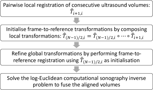
Figure 1: Overview of the method. Left: Schematic representation of the multiview acquisition. Right: Proposed flowchart.

2 Image Alignment

As illustrated in Figure 1, given a set of $N$ ultrasound volumes, we register them, using rigid transformations, to a common reference frame before we apply our spatial compounding technique. We choose the middle image of the sequence, i.e. the $(N-1)/2$ frame, as the reference image. All the images are registered to the middle image. However, direct registration between the $i$th image, where $1\leq i\leq N$, to the centre image may be difficult considering the wide difference in orientation between the images. To address this we follow the steps below to register the $i$th image and the $(N-1)/2$th image:

1. In the first step, we register neighbouring images using NiftyReg[4, 5]. We obtain $\hat{T}_{i+1,i}$ as the transformation from the $i$th image to the $(i+1)$th image, where $1\leq i<N$.

2. We initialize the transformation $T_{(N-1)/2,i}$ by composing all the intermediate transformations calculated in the previous step: $\hat{T}_{(N-1)/2,i}=\hat{T}_{(N-1)/2,((N-1)/2)-1}\circ\cdots\circ\hat{T}_{i+2,i+1}\circ\hat{T}_{i+1,i}$.

3. We refine the transformation $T_{(N-1)/2,i}$ by registering, again using NiftyReg[4, 5], the $i^{\textrm{th}}$ image and the $(N-1)/2^{\textrm{th}}$ image, starting from the transformation $\hat{T}_{(N-1)/2,i}$ from the previous step.

While this simple approach performed well in the presented experiments, further work will evaluate more elaborate registration approaches where global consistency would be achieved by registering all possible pairs of ultrasound volumes in a bundle-adjustment fashion[6] or by relying on joint registration method[7].

3 Mathematical Preliminaries

3.1 Duplication Matrix

Let $A$ be a $k\times k$ matrix. The operator $\operatorname*{vec}$ stacks the columns of a matrix into a vector. The operator $\operatorname*{unvec}$ does the inverse with $\operatorname*{unvec}({\operatorname*{vec}({A})})=A$. If $A$ is symmetric, $\operatorname*{vec}(A)$ contains duplicate information. It is therefore convenient to also consider half-vectorisation, $\operatorname*{vech}({A})$, by eliminating all supra-diagonal elements of $A$. The duplication operator[8] $\mathcal{D}:\mathbb{R}^{(k(k+1)/2)\times 1}\to\mathbb{R}^{(k^{2})\times 1}$ duplicates elements of a vector $U=\operatorname*{vech}({A})$, such that $\mathcal{D}(\operatorname*{vech}({A}))=\operatorname*{vec}({A})$. In our context where $k=3$, we obtain

$$\operatorname*{vech}({A}) =(a_{11},a_{21},a_{31},a_{22},a_{32},a_{33})^{T}$$ (1)

$$\operatorname*{vec}({A}) =(a_{11},a_{21},a_{31},a_{12},a_{22},a_{32},a_{13},a_{23},a_{33})^{T}=\mathcal{D}\cdot\operatorname*{vech}({A})$$ (2)

$$\mathcal{D} =\begin{bmatrix}1&0&0&0&0&0\\ 0&1&0&0&0&0\\ 0&0&1&0&0&0\\ 0&1&0&0&0&0\\ 0&0&0&1&0&0\\ 0&0&0&0&1&0\\ 0&0&1&0&0&0\\ 0&0&0&0&1&0\\ 0&0&0&0&0&1\\ \end{bmatrix}$$ (3)

3.2 Derivative of the Matrix Exponential

Let $M$ be a diagonalisable matrix (such as a symmetric matrice). The derivative of the matrix exponential, $M\mapsto\exp(M)$, is provided in Kalbfleisch et al.[9] and Najfeld et al.[10] as:

$$\frac{d\exp(M)}{dM}=(V\otimes V^{-T})\cdot\operatorname*{diag}({\operatorname*{vec}({L_{\exp}(\lambda)})})\cdot(V^{-1}\otimes V^{T}),$$ (4)

where $\otimes$ is the Kronecker product, $M=V\Lambda V^{-1}$ is the eigen decomposition of the matrix $M$, $\lambda$ is the vector of eigenvalues (i.e. $\Lambda=\operatorname*{diag}({\lambda})$) and $L_{\exp}(\lambda)$ is the Loewner matrix of the exponential and the vector of eigenvalues. We have:

$$L_{\exp}(\lambda)=\frac{\exp(\lambda)\oplus 1-1\oplus\exp(\lambda)}{\lambda\oplus 1-1\oplus\lambda},$$ (5)

where

$$[L_{\exp}(\lambda)]_{ij}=\left\{\begin{array}[]{ll}\exp(\lambda_{i})&\mbox{if }i=j\\ \frac{(\exp(\lambda_{i})-\exp(\lambda_{j}))}{(\lambda_{i}-\lambda_{j})}&\mbox{if }i\neq j\end{array}\right.$$ (6)

and where $\oplus$ is the Kronecker sum, i.e. $P\oplus Q=P\otimes\operatorname{Id}+\operatorname{Id}\otimes Q$. We note that using a simple Taylor expansion we obtain numerically well-behaved formulas in case of equal or minor differences between eigen values:

$$\frac{\exp(\lambda+\epsilon)-\exp(\lambda)}{\lambda+\epsilon-\lambda}=\exp(\lambda)(1+\frac{\epsilon}{2}+\frac{\epsilon^{2}}{6}+\dots)$$ (7)

Alternatively, one may also resort to one of the formulas provided by Najfeld et al.[10] for the generic case in which $M$ need not be differentiable:

$$\frac{d\exp(M)}{dM} =(\operatorname{Id}\otimes\exp(M))\frac{1-\exp(-\operatorname{ad}_{M})}{\operatorname{ad}_{M}}$$ (8)

$$=(\exp(M/2)^{T}\otimes\exp(M/2))\operatorname{sinch}(-\operatorname{ad}_{M/2})$$ (9)

with $\operatorname{ad}_{M}=(-M^{T})\oplus M$ providing the adjoint action of a matrix $M$.

4 Log-Euclidean Computational Sonography

Given a set of transformed ultrasound volumes, we obtain a composite volume where each voxel is a $3\times 3$ tensor by minimizing the following term as suggested in Hennersperger et al.[1],

$$\operatorname*{arg\,min}_{Q_{j}}\sum_{i}\sum_{j}(v_{i}^{T}Q_{j}v_{i}-I_{ij})^{2},$$ (10)

where $Q_{j}$ is the symmetric tensor at voxel location $j$, $1\leq j\leq m$, m is the number of voxels, $1\leq i\leq n$, $n$ is the number of images, $v_{i}$ is the directional vector or probe direction of the $i$th ultrasound volume and $I_{ij}$ is the voxel intensity. As pointed out in Hennersperger et al.[1], solving the above equation without specific constraints on $Q_{j}$ may lead to a non positive definite tensor. To ensure a positive definite tensor $Q_{j}$, we re-write the above equation using the log-Euclidean approach of Arsigny et al.[11]. With this approach, positive definite tensors $Q_{j}$ are parameterised with arbitrary symmetric matrices $S_{j}$ through the use of the matrix exponential $Q_{j}=\exp(S_{j})$. The operators $\operatorname*{unvec}$ and $\mathcal{D}$ enables us to write the symmetric $3\times 3$ matrices $S_{j}$ in a parametric form without redundancies using a vector $X_{j}\in\mathbb{R}^{6\times 1}$: $S_{j}=\operatorname*{unvec}({\mathcal{D}\cdot X_{j}})$.

We additionally introduce a robust loss function $\rho$ and a total variation penalisation term to regularise the ill-posed problem while preserving edge information. We obtain the following variational problem:

$$\operatorname*{arg\,min}_{X_{j}}\sum_{i}\sum_{j}\rho((v_{i}^{T}\exp(\operatorname*{unvec}({\mathcal{D}\cdot X_{j}}))v_{i}-I_{ij})^{2})+\lambda\cdot\operatorname*{TV}({X_{j}}).$$ (11)

A smooth approximation of the total variation regularisation term can be provided by relying on the Huber loss function, as exemplified in the 1D case below:

$$\operatorname*{TV^{H}}(x)=\begin{cases}\tfrac{1}{2}(\nabla x)^{2}&\text{if }|\nabla x|\leq\delta\\ \delta(|\nabla x|-\tfrac{1}{2}\delta)&\text{otherwise}\end{cases}$$ (12)

Equation (11) becomes a non-linear least squares problem that can efficiently be solved if one can compute the Jacobian of the residuals. In this work, we make use of the Levenbeg-Marquardt algorithm[12] available in the Ceres Solver library[13]. The first term of (11) can be rewritten using

$$f(X_{j})=\Phi(\exp(\operatorname*{unvec}({\mathcal{D}\cdot X_{j}}))),$$ (13)

where

$$\Phi(A_{j})=v_{i}^{T}A_{j}v_{i}-I_{ij}.$$ (14)

Using the chain rule, the Jacobian of $f$ is given as,

$$J_{f}(X)=J_{\Phi}(\exp(\operatorname*{unvec}({\mathcal{D}\cdot X})))\cdot J_{\exp}(\operatorname*{unvec}({\mathcal{D}\cdot X}))\cdot J_{\operatorname*{unvec}}{(\mathcal{D}\cdot X)}\cdot J_{\mathcal{D}}\cdot X=v_{i}\otimes v_{i}\cdot\frac{d\exp(M)}{dM}\cdot 1\cdot\mathcal{D}.$$ (15)

Combining the terms, the Jacobian of $f$ is given as,

$$J_{f}(X)=(v_{i}\otimes v_{i})\cdot(V\otimes V^{-T})\cdot\operatorname*{diag}({\operatorname*{vec}({L_{\exp}(\lambda)})})\cdot(V^{-1}\otimes V^{T})\cdot\mathcal{D}.$$ (16)

We highlight that even though the model (11) provided interesting results in our experiment, future work would need to model more realistically the physics of ultrasound image acquisition including signal attenuation, and scattering. This could, in the first instance, be done using an effective but computationally tractable model such as the one presented by Wein et al.[14] for CT-Ultrasound registration.

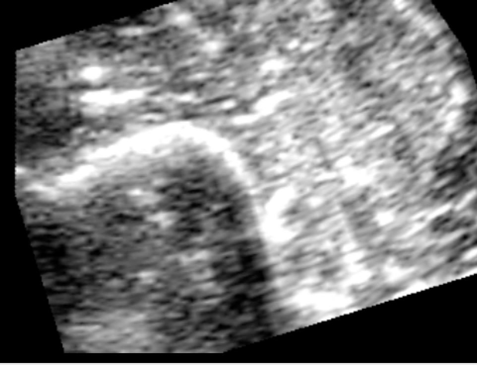
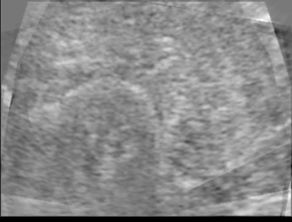
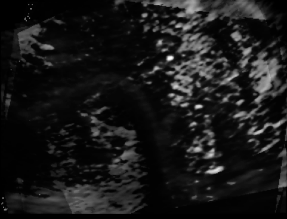
(a) Dataset 1 - 2nd image out of a sequence of nine images

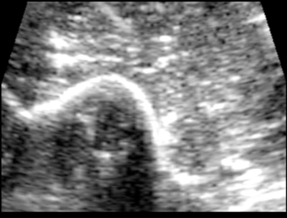
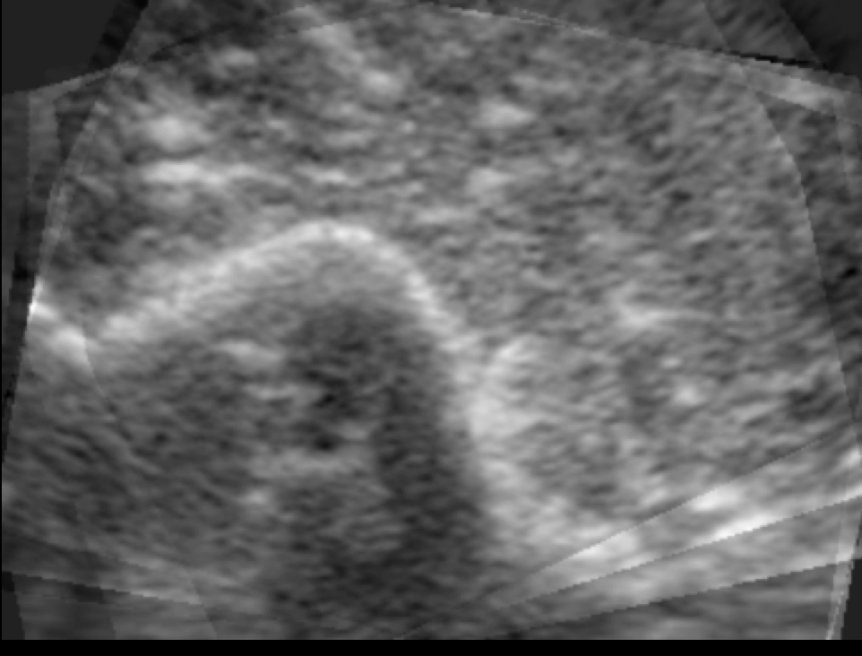
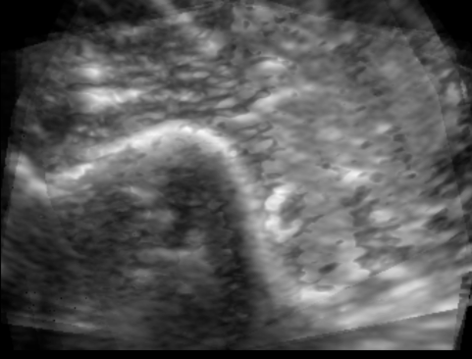
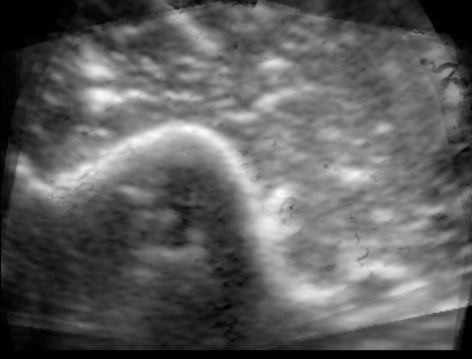
(b) Dataset 1 - 5th image out of a sequence of nine images

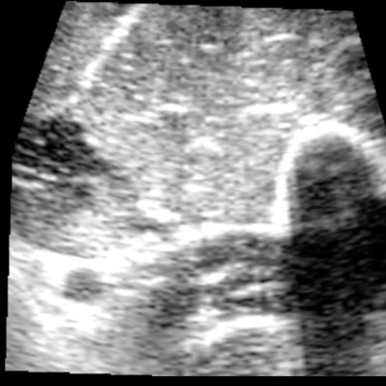
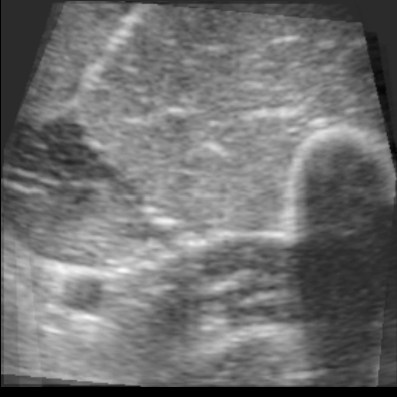
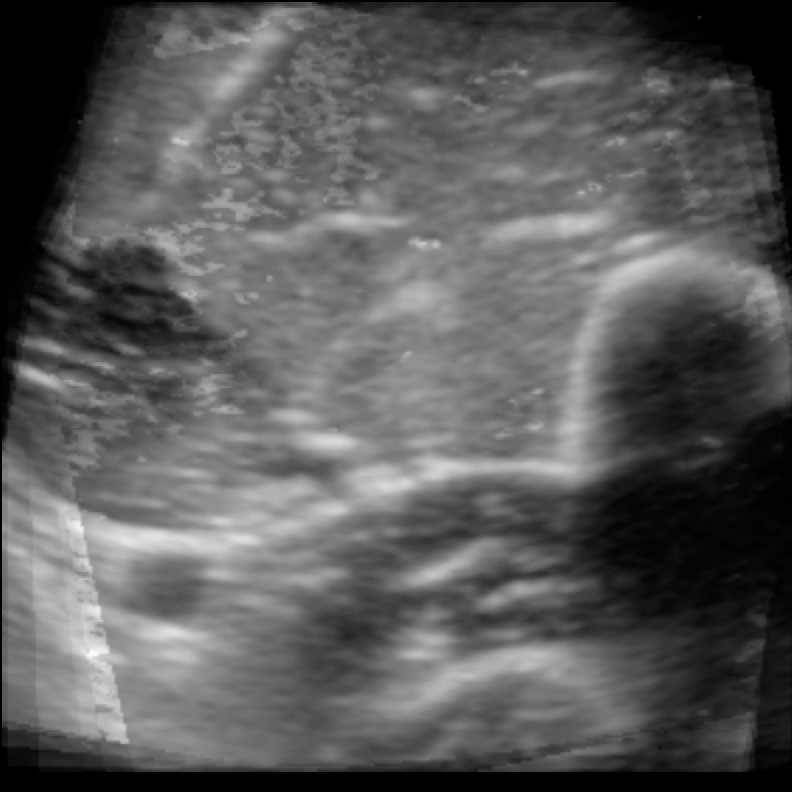
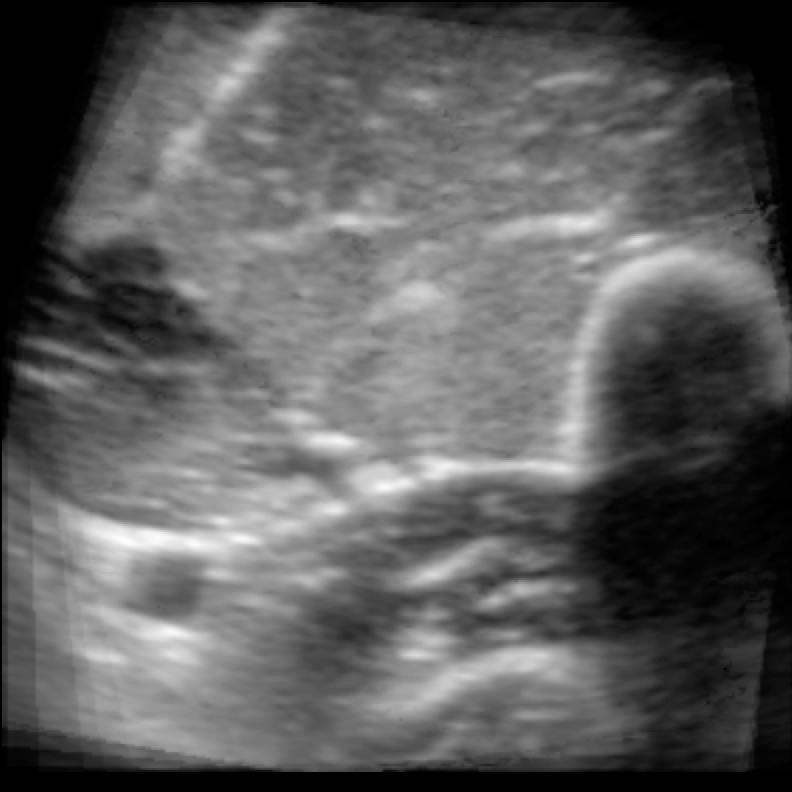
(c) Dataset 2 - 6th image out of a sequence of nine images

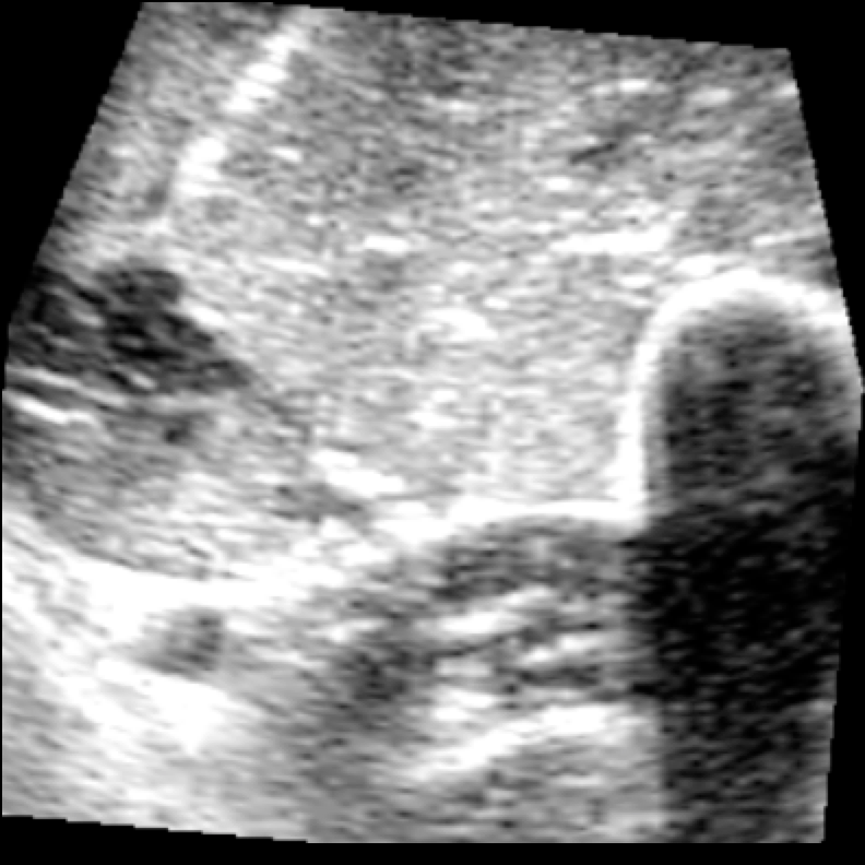
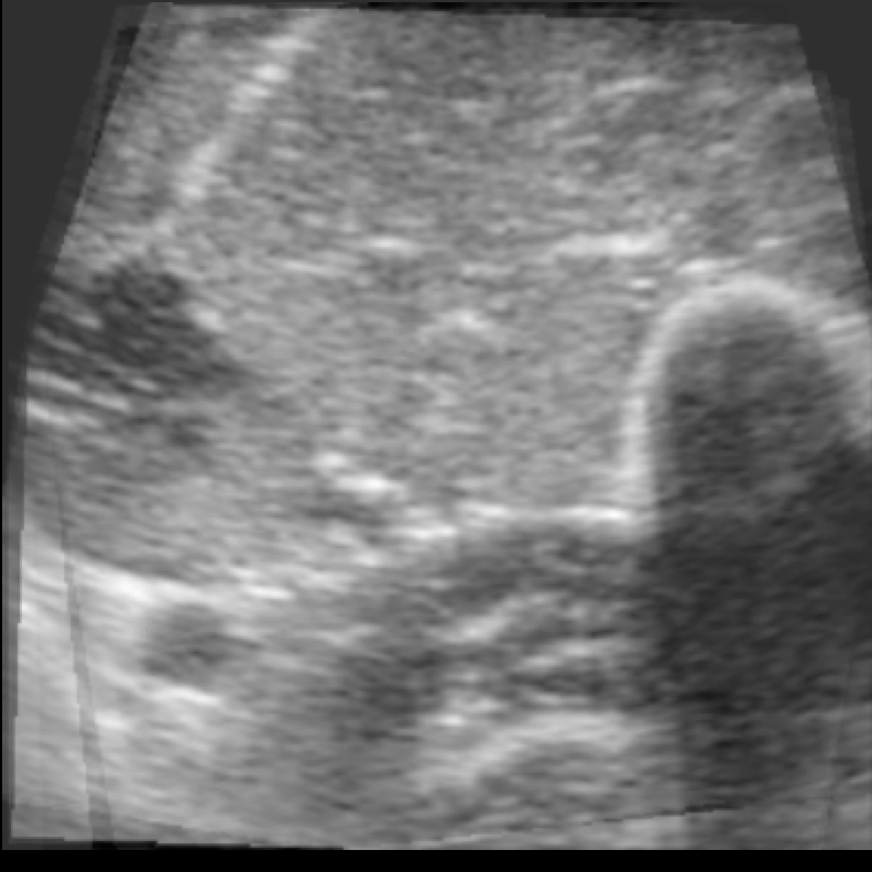
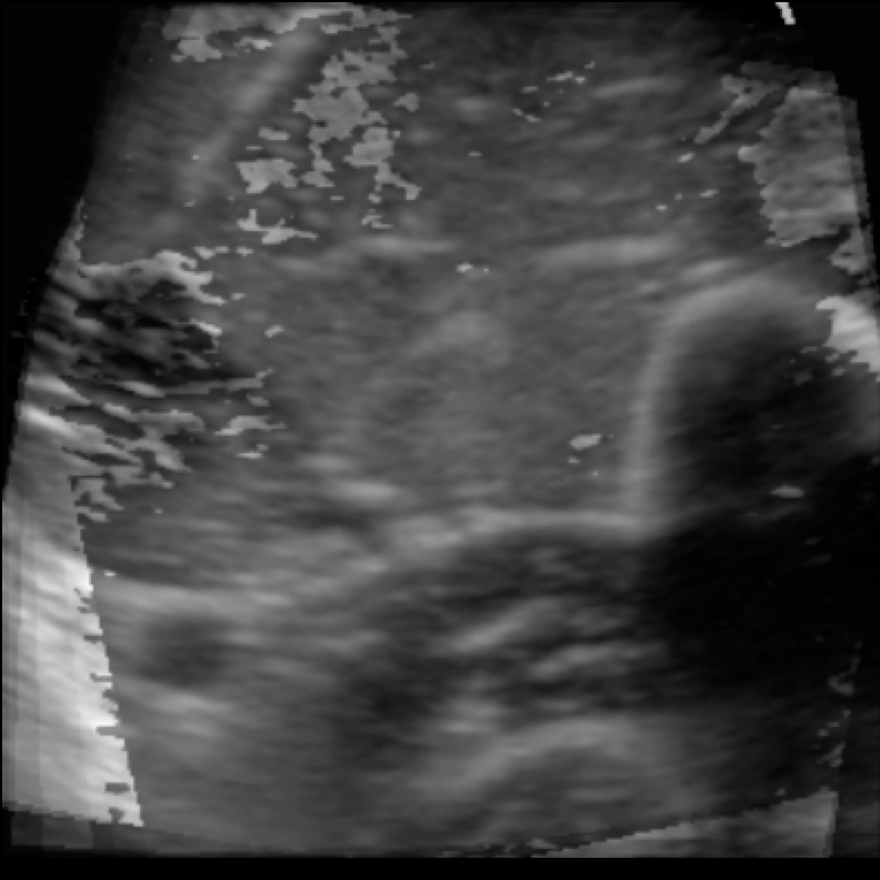
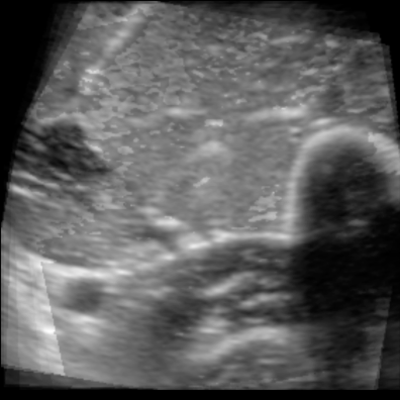
(d) Dataset 2 - 7th image out of a sequence of nine images

Figure 2: The four column from left to right are as follows: (1) Leave-one-out image, (2) Hennersperger et al.[1], (3) Our method $\lambda$ = 0 and, (4) Our method $\lambda$ = 10.

5 Results

We evaluated the proposed method on in vivo human datasets. The ultrasound datasets were acquired from two volunteers. Consent was obtained before ultrasound acquisition. Ultrasound acquisition was performed using a Voluson E10 ultrasound system with an eM6C curved matrix electronic 4D transducer (GE Healthcare, Chicago, Il). Each dataset contained nine (N = 9) volumes. The probe was gradually translated over the body surface whilst tilting to maintain the target body part in the field of view. We use peak signal to noise ratio (PSNR) as the evaluation metric.

Table 1: PSNR Leave-one-out results (in dB).

Dataset	Hennersperger et al.[1]	Our method
		$\lambda$ = 0	$\lambda$ = 1	$\lambda$ = 10	$\lambda$ = 100
1	18.8	16.1	21.2	21.6	13.6
2	17.5	17.7	21.8	22.6	22.9

The two parameters in (11) are $\lambda$ and $\delta$. $\lambda$ is the scale factor and $\delta$ is the constant in the Huber loss function. $\lambda$ is evaluated for the following set of values: 0, 1, 10 and 100. The constant $\delta$ was set to a small positive value ($\delta=0.01$).

We used leave-one-out strategy to evaluate the performance of the method. In each round of the leave-one-out we leave out one of the images from the set of N images. We then estimate the tensor image using the rest of the N-1 images. The estimated tensor image is used to generate the projection image along the direction of the left out image. The projection image is then compared to the left out image using the PSNR metric. This is iterated over all the images in the set. The results are averaged over all the round to estimate the overall error, see Table 1. Table 1 shows that our method performs better than Hennersperger et al.[1]. As per the leave-one-out rounds in Table 1, $\lambda$ = 10 is the best parameter setting. Some of the leave-one-out results are shown in Figure 2. In Figure 2, the images on the left columns are the leave-one-out images, the second to left column are the output images using Hennersperger et al.[1], the third to left column are the output images using our method with parameter $\lambda$ = 0, and the last column at the right are the output images using our method with parameter $\lambda$ = 10.

6 Conclusion

We propose a spatial compounding technique to improve the 3D ultrasound image quality by compositing multiple ultrasound volumes acquired from different probe orientations. Our compounding technique uses a tensor representation which is sensitive to the probe orientation. The proposed method has a better PSNR than Hennersperger et al.[1] which uses similar tensor based representation. The log-Euclidean framework ensures that the tensors are positive definite, enforcing a non-negative image. The additional total variation term is used for spacial regularisation. The initial results of the proposed method are promising. Future work will focus on improving the validation of our methods, on introducing more realistic models of signal attenuation and on providing a combined method to jointly optimise the image alignment and the tensor model fitting.

- [1] Hennersperger, C., Baust, M., Mateus, D., and Navab, N., “Computational sonography,” Medical Image Computing and Computer-Assisted Intervention - MICCAI 2015 - 18th International Conference Munich, Germany, October 5-9, 2015, Proceedings, Part II , 459–466 (2015).
- [2] Wachinger, C., Wein, W., and Navab, N., “Three-dimensional ultrasound mosaicing,” MICCAI (2) , 327–335 (2007).
- [3] Kutarnia, J. and Pedersen, P. C., “3D seam selection techniques with application to improved ultrasound mosaicing,” Medical Imaging 2013: Image Processing, Lake Buena Vista (Orlando Area), Florida, USA, February 10-12, 2013 , 866949 (2013).
- [4] Ourselin, S., Roche, A., Prima, S., and Ayache, N., “Block matching: A general framework to improve robustness of rigid registration of medical images,” Medical Image Computing and Computer-Assisted Intervention - MICCAI 2000, Third International Conference, Pittsburgh, Pennsylvania, USA, October 11-14, 2000, Proceedings , 557–566 (2000).
- [5] Modat, M., Cash, D. M., Daga, P., Winston, G. P., Duncan, J. S., and Ourselin, S., “Global image registration using a symmetric block-matching approach,” Journal of Medical Imaging 1, 1 – 1 – 6 (2014).
- [6] Vercauteren, T., Perchant, A., Malandain, G., Pennec, X., and Ayache, N., “Robust mosaicing with correction of motion distortions and tissue deformation for in vivo fibered microscopy,” Medical Image Analysis 10(5), 673–692 (2006).
- [7] Zöllei, L., Learned-Miller, E. G., Grimson, W. E. L., and Wells III, W. M., “Efficient population registration of 3d data,” CVBIA , 291–301 (2005).
- [8] Magnus, J. R. and Neudecker, H., “Symmetry, 0-1 matrices, and Jacobians: a review,” Econometric Theory 2, 157–190 (Aug. 1986).
- [9] Kalbfleisch, J. and Lawless, J., “The analysis of panel data under a Markov assumption,” Journal of the American Statistical Association 80(392) (1985).
- [10] Najfeld, I. and Havel, T. F., “Derivatives of the matrix exponential and their computation,” Advances in Applied Mathematics 16, 321–375 (Sept. 1995).
- [11] Arsigny, V., Fillard, P., Pennec, X., and Ayache, N., “Log-Euclidean metrics for fast and simple calculus on diffusion tensors,” Magnetic Resonance in Medicine 56, 411–421 (Aug. 2006).
- [12] Madsen, K., Nielsen, H. B., and Tingleff, O., “Methods for non-linear least squares problems (2nd ed.),” (2004).
- [13] Agarwal, S., Mierle, K., and Others, “Ceres solver.” http://ceres-solver.org.
- [14] Wein, W., Brunke, S., Khamene, A., Callstrom, M. R., and Navab, N., “Automatic CT-ultrasound registration for diagnostic imaging and image-guided intervention,” Medical Image Analysis 12(5), 577–585 (2008).