Heavy meson dissociation in a plasma with magnetic fields

Abstract

The fraction of heavy vector mesons detected after a heavy ion collision provides information about the possible formation of a plasma state. An interesting framework for estimating the degree of dissociation of heavy mesons in a plasma is the holographic approach. It has been recently shown that a consistent picture for the thermal behavior of charmonium and bottomonium states in a thermal medium emerges from holographic bottom up models. A crucial ingredient in this new approach is the appropriate description of decay constants, since they are related to the heights of the quasiparticle peaks of the finite temperature spectral function.

Here we extend this new holographic model in order to study the effect of magnetic fields on the thermal spectrum of heavy mesons. The motivation is that very large magnetic fields are present in non central heavy ion collisions and this could imply a change in the dissociation scenario. The thermal spectra of $c\bar{c}$ and $b\bar{b}\,$ S wave states is obtained for different temperatures and different values of the magnetic $eB$ field.

I Introduction

A consistent picture for the thermal behavior of heavy vector mesons in a plasma was obtained recently using holographic bottom up modelsBraga:2016wkm ; Braga:2017oqw ; Braga:2017bml . A central point in these works is the connection between the finite temperature spectral function and the zero temperature decay constants. The spectral function – that describes the thermal behavior of quasiparticles inside a thermal medium – is the imaginary part of the retarded Green’s function. At zero temperature, the essential part of the Green’s function has the following spectral decomposition in terms of masses $m_{n}$ and decay constants $f_{n}$ of the states:

$$\Pi(p^{2})\sim\sum_{n=1}^{\infty}\,\frac{f_{n}^{2}}{(-p^{2})-m_{n}^{2}+i\epsilon}\,.$$ (1)

The imaginary part of this expression is a sum of Dirac deltas with coefficients proportional to the square of the decay constants: $f_{n}^{2}\,\delta(-p^{2}-m_{n}^{2})$. At finite temperature, the quasi-particle states appear in the spectral function as smeared – finite size – peaks with a height that decrease as the temperature $T$ and/or the density $\mu$ of the medium increase. This analysis strongly suggests that in order to extend a hadronic model to finite temperature, the zero temperature case should provide a consistent description of decay constants.

Decay constants for mesons are associated with non-hadronic decay. They are proportional to the transition matrix from a state at excitation level $n$ to the hadronic vacuum: $\langle 0|\,J_{\mu}(0)\,|n\rangle=\epsilon_{\mu}f_{n}m_{n}$. Experimental data show that for heavy vector mesons the decay constants decrease monotonically with radial excitation level, as revised in Braga:2017oqw ; Braga:2017bml .

Holographic models, inspired in the AdS/CFT correspondenceMaldacena:1997re ; Gubser:1998bc ; Witten:1998qj , provide nice estimates for hadronic masses. However neither the hard wall Polchinski:2001tt ; BoschiFilho:2002ta ; BoschiFilho:2002vd , the soft wall Karch:2006pv or the D4-D8 Sakai:2004cn models provide decay constants decreasing with excitation level.

An alternative bottom up holographic model was developed in ref. Braga:2015jca in order to overcome this problem. The decay constants are obtained from two point correlators of gauge theory operators calculated at a finite value of the radial coordinate of AdS space. This way an extra energy parameter, associated with an ultraviolet (UV) energy scale, is introduced in the model. The extension of this model to finite temperature in Braga:2016wkm and finite density in Braga:2017oqw provided consistent pictures for the dissociation of heavy vector mesons is the plasma. An improved version of the model of ref. Braga:2015jca , that provides a better fit for the charmonium states at zero temperature and thus a better picture for the finite temperature and density cases, was then proposed in Braga:2017bml .

An interesting tool to investigate the possible existence of a plasma state in a heavy ion collision is to analyze the fraction of heavy vector mesons produced. The suppression of such particles indicates their dissociation in the mediumMatsui:1986dk (see also Satz:2005hx ). This effect corresponds to a decrease in the height of the quasi particle peaks of the spectral function. The influence of temperature and density of the medium in heavy vector meson spectral functions was studied in Braga:2016wkm ; Braga:2017oqw ; Braga:2017bml . However, there is another important factor that deserves consideration. In non central heavy ion collisions strong magnetic fields can be produced for short time scalesKharzeev:2007jp ; Fukushima:2008xe ; Skokov:2009qp .

The presence of a magnetic field $eB$ has important consequences for hadronic matter. Lattice results Bali:2011qj indicate a decrease in the QCD deconfinement temperature with increasing $eB$ field. Similar results show up also from the MIT bag modelFraga:2012fs and also from the holographic D4-D8 modelBallon-Bayona:2013cta . The effect of a magnetic field in the transition temperature of a plasma has been studied using holographic models in many works, as for example Mamo:2015dea ; Dudal:2015wfn ; Evans:2016jzo ; Li:2016gfn ; Ballon-Bayona:2017dvv ; Rodrigues:2017cha .

Here we extend the holographic bottom up model of Braga:2017bml in order to include the presence of a magnetic field. This way it is possible to investigate the change in the spectral function peaks that represent the quasiparticle heavy meson states as a function of the intensity of the $eB$ field. In section II we describe the model at zero temperature showing the results for masses and decay constants. Then, in section III we present the extension to finite temperature in the presence of a magnetic field. Section IV is devoted to show how to calculate the spectral functions. Finally, in section V we present the results as discuss their implication in terms of heavy vector meson dissociation.

II Holographic Model

The model proposed in ref.Braga:2017bml was conceived for describing charmonium states. At zero temperature the background geometry is the standard 5D anti-de Sitter space-time

$$ds^{2}\,\,=\,\,\frac{R^{2}}{z^{2}}(-dt^{2}+d\vec{x}\cdot d\vec{x}+dz^{2})\,.$$ (2)

The mesons are described by a vector field $V_{m}=(V_{\mu},V_{z})\,$ ($\mu=0,1,2,3$), which is dual to the gauge theory current $J^{\mu}=\bar{\psi}\gamma^{\mu}\psi\,$. The action is:

$$I\,=\,\int d^{4}xdz\,\sqrt{-g}\,\,e^{-\phi(z)}\,\left\{-\frac{1}{4g_{5}^{2}}F_{mn}F^{mn}\,\right\}\,\,,$$ (3)

where $F_{mn}=\partial_{m}V_{n}-\partial_{n}V_{m}$ and $\phi(z)$ is a background dilaton field that here we choose to have the form

$$\phi(z)=k^{2}z^{2}+Mz+\tanh\left(\frac{1}{Mz}-\frac{k}{\sqrt{\Gamma}}\right)\,,$$ (4)

in order to represent both charmonium and bottomonium states. The parameter $k$ represents the quark mass, $\Gamma$ the string tension of the strong quark anti-quark interaction and $M$ is a mass scale associated with non hadronic decay.

Choosing the gauge $V_{z}=0$ the equation of motion for the transverse (1,2,3) components of the field, denoted generically as $V$, in momentum space reads

$$\partial_{z}\left[e^{-B(z)}\partial_{z}V\right]-p^{2}e^{-B(z)}V=0,$$ (5)

where $B(z)$ is

$$B(z)=\log\left(\frac{z}{R}\right)+\phi(z)\,.$$ (6)

Equation of motion (5) presents a discrete spectrum of normalizable solutions, $V(p,z)=\Psi_{n}(z)$ that satisfy the boundary conditions $\Psi_{n}(z=0)=0$ for $p^{2}=-m_{n}^{2}$ where $m_{n}$ are the masses of the corresponding meson states. The eigenfunctions $\Psi_{n}(z)$ are normalized according to:

$$\int^{\infty}_{0}dz\ e^{-B(z)}\ \Psi_{n}(z)\Psi_{m}(z)=\delta_{mn}\,.$$ (7)

Decay constants are proportional to the transition matrix from the vector meson $n$ excited state to the vacuum: $\langle 0|\,J_{\mu}(0)\,|n\rangle=\epsilon_{\mu}f_{n}m_{n}$. They are calculated holographically in the same way as in the soft wall model:

$$f_{n}=\frac{1}{g_{5}m_{n}}\lim\limits_{z\rightarrow 0}\left(e^{-B(z)}\Psi_{n}(z)\right)\,.$$ (8)

The values of the parameters that describe charmonium and bottomonium are respectively:

$$k_{c}=1.2\,{\rm GeV};\,\,\sqrt{\Gamma_{c}}=0.55\,{\rm GeV};\,\,M_{c}=2.2\,{\rm GeV}\,;$$ (9)

$$k_{B}=2.45\,{\rm GeV};\,\,\sqrt{\Gamma_{B}}=1.55\,{\rm GeV};\,\,M_{B}=6.2\,{\rm GeV}\,.$$ (10)

The procedure to calculate masses and decay constants is to find the normalizable solutions $\Psi_{n}(z)$ of eq. (5), with the background of eq. (4), that vanish at $z=0$. Then the numerical solutions are used in eq. (8). Tables 1 and 2 show the results for charmonium and bottomonium respectively. For comparison, the experimental data from ref. (Agashe:2014kda ) is show inside parenthesis. Note that the decay constants decrease with radial excitation level.

Holographic (and experimental) Results for Charmonium
State	Mass (MeV)	Decay constants (MeV)
$\,\,\,\,1S\,\,\,\,$	$2943\,\,(3096.916\pm 0.011)$	$399\,(416\pm 5.3)$
$\,\,\,\,2S\,\,\,\,$	$3959\,\,(3686.109\pm 0.012)$	$255\,(296.1\pm 2.5)$
$\,\,\,\,3S\,\,\,\,$	$4757\,\,(4039\pm 1)$	$198\,(187.1\pm 7.6)$
$\,\,\,\,4S\,\,\,\,$	$5426\,\,(4421\pm 4)$	$169\,(160.8\pm 9.7)$

Table 1: Holographic masses and the corresponding decay constants for the Charmonium S-wave resonances. Experimental values inside parenthesis for comparison.

Holographic (and experimental) Results for Bottomonium
State	Mass (MeV)	Decay constants (MeV)
$\,\,\,\,1S\,\,\,\,$	$6905\,\,(9460.3\pm 0.26)$	$719\,(715.0\pm 2.4)$
$\,\,\,\,2S\,\,\,\,$	$8871\,(10023.26\pm 0.32)$	$521\,(497.4\pm 2.2)$
$\,\,\,\,3S\,\,\,\,$	$10442\,\,(10355.2\pm 0.5)$	$427\,(430.1\pm 1.9)$
$\,\,\,\,4S\,\,\,\,$	$11772\,(10579.4\pm 1.2)$	$375\,(340.7\pm 9.1)$

Table 2: Holographic masses and the corresponding decay constants for the Bottomonium S-wave resonances. Experimental values inside parenthesis for comparison.

III Plasma with magnetic field

Let us now extend the model to finite temperature and in the presence of magnetic field, assumed for simplicity to be constant in time and homogeneous in space. The extension to finite temperature is obtained replacing AdS space by a Schwarzschild AdS black hole. The presence of a magnetic field in the gauge theory side of gauge/gravity duality can also be represented geometrically in the gravity sideDHoker:2009mmn ; DHoker:2009ixq . The Einstein-Maxwell action is given by:

$$S=\frac{1}{16\pi G_{5}}\int d^{5}x\sqrt{-g}\left(R-F^{MN}F_{MN}+\frac{12}{L^{2}}\right)+S_{GH}$$ (11)

with $F_{MN}$ is the electromagnetic field strength, $R$ is the Ricci scalar and $\Lambda$=$\,-\frac{12}{L^{2}}$ is the negative cosmological constant. The second term in eq. (11) is the Gibbons-Hawking surface term.

The equations of motion obtained from eq.(11) are

$$R_{MN}= - \frac{4}{L^{2}}g_{MN}-\frac{g_{MN}}{3}F^{PQ}F_{PQ}+2F_{MP}F_{\,\,\,N}^{P},$$ (12)

$$\nabla_{M}F_{MN}=0.$$ (13)

In order to represent a magnetic field $eB$ we will use a Black hole solution studied in Dudal:2015wfn

$$ds^{2}\,\,=\,\,\frac{R^{2}}{z^{2}}\,\Big{(}-f(z)dt^{2}+\frac{dz^{2}}{f(z)}+(dx_{1}^{2}+dx_{2}^{2})d(z)+dx_{3}^{2}q(z)\Big{)}\,.$$ (14)

In this expression the factors are

$$f(z)=1-\frac{z^{4}}{z_{h}^{4}}+\frac{2}{3}\frac{e^{2}B^{2}z^{4}}{1.6^{2}}\ln\left(\frac{z}{z_{h}}\right)\,,$$ (15)

$$q(z)=1+\frac{8}{3}\frac{e^{2}B^{2}}{1.6^{2}}\int^{1/z}_{+\infty}dx\frac{\ln{(z_{h}z)}}{z^{3}(z^{2}-\frac{1}{z_{h}^{4}x^{2}})}.$$ (16)

$$d(z)=1-\frac{4}{3}\frac{e^{2}B^{2}}{1.6^{2}}\int^{1/z}_{+\infty}dx\frac{\ln{(z_{h}z)}}{z^{3}(z^{2}-\frac{1}{z_{h}^{4}x^{2}})}.$$ (17)

where $z_{h}$ is the horizon position and $eB$ is the boundary magnetic field that is in the $x_{3}$ direction. The temperature of the black hole and of the gauge theory is:

$$T=\frac{|f^{\prime}(z)|_{(z=z_{h})}}{4\pi}=\frac{1}{4\pi}\left|\frac{4}{z_{h}}-\frac{2}{3}e^{2}B^{2}z_{h}^{3}\right|\,.$$ (18)

We assume that the geometry is not modified by the presence of the dilaton background. So, the action has the same form of eq. (3) with the dilaton background $\phi(z)$ of eq. (4) but with metric the (14). Now the equations of motion have to be solved numerically. In the next section we discuss how to solve them with the appropriate boundary conditions using the membrane paradigm.

IV Spectral Function

The spectral functions for heavy vector mesons will be calculated using the membrane paradigm Iqbal:2008by (see also Finazzo:2015tta ). Let us see how this formalism works for a vector field $V_{\mu}$ in the bulk, dual to the electric current operator $J_{\mu}$. We consider a general black brane background of the form

$$ds^{2}=-g_{tt}dt^{2}+g_{zz}dz^{2}+g_{x_{1}x_{1}}dx^{2}_{1}+g_{x_{2}x_{2}}dx^{2}_{2}+g_{x_{3}x_{3}}dx^{2}_{3}\,,$$ (19)

where we assume the boundary is at a position $z=0$ and the horizon position $z=z_{h}$ is given by the root of $g_{tt}(z_{h})=0$. The bulk action for the vector field is

$$S=-\int d^{5}x\,\sqrt{-g}\frac{1}{4g_{5}^{2}\,h(z)}F^{mn}F_{mn}\,,$$ (20)

where $h(z)$ is a z-dependent coupling. The equation of motion that follows from this action is:

$$\partial^{m}\left(\frac{\sqrt{-g}}{h(z)}F_{mn}\right)=0\,.$$ (21)

The conjugate momentum to the gauge field with respect to a foliation by constant z-slices is given by:

$$j^{\mu}=-\frac{1}{h(z)}\sqrt{-g}F^{z\mu}\,.$$ (22)

We assume that the metric (19) satisfies $g_{x_{1}x_{1}}=g_{x_{2}x_{2}}$ that includes our case of interest: metric (14) that represents a magnetic field in the $x_{3}$ direction. We also assume solutions for the vector field that do not depend on the coordinates $x_{1}$ and $x_{2}$, like a plane wave with spatial momentum in the $x_{3}$ direction. Equations of motion (21) can be separated in two different channels: a longitudinal one involving fluctuations along $(t,x_{3})$ and a transverse channel involving fluctuations along spatial directions $(x_{1},x_{2})$. Using eq. (22), the components $t$, $x_{3}$ and $z$ of eq. (21) can be written respectively as

$$-\partial_{z}j^{t}-\frac{\sqrt{-g}}{h}g^{tt}g^{x_{3}x_{3}}\partial_{x_{3}}F_{x_{3}t}=0\,,$$ (23)

$$-\partial_{z}j^{x_{3}}+\frac{\sqrt{-g}}{h}g^{tt}g^{x_{3}x_{3}}\partial_{t}F_{x_{3}t}=0\,,$$ (24)

$$\partial_{x_{3}}j^{x_{3}}+\partial_{t}j^{t}=0\,.$$ (25)

From the Bianchi identity one finds the relation:

$$\partial_{z}F_{x_{3}t}-\frac{h(z)}{\sqrt{-g}}g_{zz}g_{x_{3}x_{3}}\partial_{t}j^{z}-\frac{h(z)}{\sqrt{-g}}g_{tt}g_{x_{3}x_{3}}\partial_{x_{3}}j^{t}=0\,.$$ (26)

Now, one can define a z-dependent ”conductivity” for the longitudinal channel given by:

$$\bar{\sigma}_{L}(\omega,\vec{p},z)=\frac{j^{x_{3}}(\omega,\vec{p},z)}{F_{x_{3}t}(\omega,\vec{p},z)}\,.$$ (27)

Taking a derivative of eq. (27) one finds:

$$\partial_{z}\bar{\sigma}_{L}=\frac{\partial_{z}j^{x_{3}}}{F_{x_{3}t}}-\frac{j^{x_{3}}}{F_{x_{3}t}^{2}}\partial_{z}F_{x_{3}t}\,.$$ (28)

Now using eqs. (23), (25) and (26) and considering a plane wave solution with momentum $p=(\omega,0,0,p_{3})$, the previous equation for $\bar{\sigma}_{L}$ becomes

$$\partial_{z}\bar{\sigma}_{L}=-i\omega\sqrt{\frac{g_{zz}}{g_{tt}}}\left[\Sigma_{L}(z)-\frac{\bar{\sigma}_{L}^{2}}{\Sigma_{L}(z)}\left(1-\frac{p_{3}^{2}}{\omega^{2}}\frac{g^{x_{3}x_{3}}}{g^{tt}}\right)\right]\,,$$ (29)

where

$$\Sigma_{L}(z)=\frac{1}{h(z)}\sqrt{\frac{-g}{g_{zz}g_{tt}}}g^{x_{3}x_{3}}\,.$$ (30)

Similarly, the transverse channel is governed by a dynamical equation

$$-\partial_{z}j^{x_{1}}-\frac{\sqrt{-g}}{h(z)}g^{tt}g^{x_{1}x_{1}}\partial_{t}F_{tx_{1}}+\frac{\sqrt{-g}}{h(z)}g^{x_{3}x_{3}}g^{x_{1}x_{1}}\partial_{x_{3}}F_{x_{3}x_{1}}=0\,.$$ (31)

and two constraints from the Bianchi identity

$$\partial_{z}F_{x_{1}t}-\frac{h(z)}{\sqrt{-g}}g_{zz}g_{x_{1}x_{1}}\partial_{t}j^{x_{1}} = 0\,,$$

$$\partial_{x_{3}}F_{tx_{1}}+\partial_{t}F_{x_{1}x_{3}} = 0\,.$$ (32)

One can define a z-dependent ”conductivity” also for the transverse channel:

$$\bar{\sigma}_{T}(\omega,\vec{p},z)=\frac{j^{x_{1}}(\omega,\vec{p},z)}{F_{x_{1}t}(\omega,\vec{p},z)}\,.$$ (33)

Following the same procedure used for the longitudinal channel, using eqs. (31-IV) one finds the equation for $\bar{\sigma}_{T}$:

$$\partial_{z}\bar{\sigma}_{T}=i\omega\sqrt{\frac{g_{zz}}{g_{tt}}}\left[\frac{\bar{\sigma}_{T}^{2}}{\Sigma_{T}(z)}-\Sigma_{T}(z)\left(1-\frac{p_{3}^{2}}{\omega^{2}}\frac{g^{x_{3}x_{3}}}{g^{tt}}\right)\right]\,.$$ (34)

where

$$\Sigma_{T}(z)=\frac{1}{h(z)}\sqrt{\frac{-g}{g_{zz}g_{tt}}}g^{x_{1}x_{1}}\,.$$ (35)

In the zero momentum limit, the equations (29) and (34) became respectively:

$$\partial_{z}\bar{\sigma}_{L}=i\omega\sqrt{\frac{g_{zz}}{g_{tt}}}\left[\frac{\bar{\sigma}_{L}^{2}}{\Sigma_{L}(z)}-\Sigma_{L}(z)\right]\,,$$ (36)

$$\partial_{z}\bar{\sigma}_{T}=i\omega\sqrt{\frac{g_{zz}}{g_{tt}}}\left[\frac{\bar{\sigma}_{T}^{2}}{\Sigma_{T}(z)}-\Sigma_{T}(z)\right]\,.$$ (37)

Using the Kubo’s formula it is possible relate the $z=0$ values of the five dimensional “conductivity” to the retarded Green’s function:

$$\sigma_{L}(\omega)=-\frac{G_{R}^{L}(\omega)}{i\omega}\equiv\bar{\sigma}_{L}(\omega,0)\,.$$ (38)

$$\sigma_{T}(\omega)=-\frac{G_{R}^{T}(\omega)}{i\omega}\equiv\bar{\sigma}_{T}(\omega,0)\,.$$ (39)

where $\sigma_{T}$ is the AC conductivity in transverse channel and $\sigma_{L}$ is the AC conductivity in longitudinal channel.

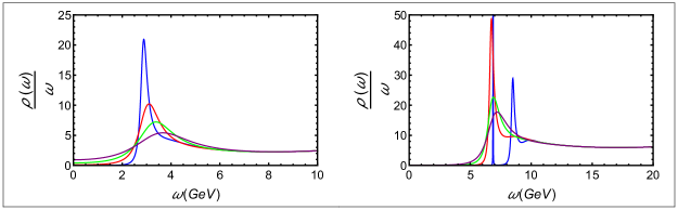
Figure 1: Spectral functions for charmonium (left panel) and bottomonium (right panel) at 4 representative values of the temperature: blue line T=195 MeV ; red line T =330 MeV; green line T = 465 MeV; purple line T = 600 MeV.

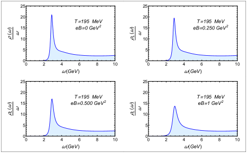
Figure 2: Spectral functions for charmonium at T= 195 MeV for different values of a magnetic field parallel to the polarization

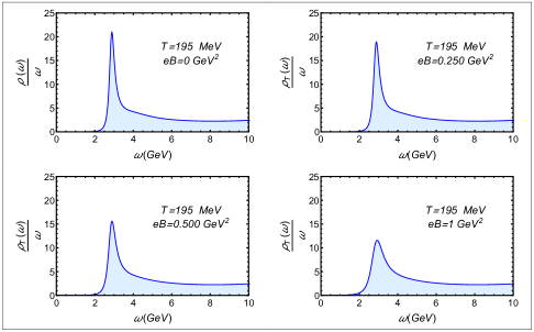
Figure 3: Spectral functions for charmonium at T= 195 MeV for different values of a magnetic field perpendicular to the polarization

In order to apply the membrane paradigm to the model of the previous section, we use the metric (14) and $h(z)=e^{\phi(z)}$, with $\phi(z)$ defined in eq. (4), in the flow equations (36) and (37). The anisotropic metric (14) leads to two different conductivities Rebhan:2011vd :

$$\partial_{z}\bar{\sigma}_{L}(\omega,z)=\frac{i\omega}{f(z)\bar{\Sigma}_{L}(z)}\left[\bar{\sigma}_{L}(\omega,z)^{2}-\bar{\Sigma}_{L}(z)^{2}\right]\,,$$ (40)

with $\bar{\Sigma}_{L}(z)=\frac{d(z)}{\sqrt{q(z)}}e^{-\phi(z)}/z$ and

$$\partial_{z}\bar{\sigma}_{T}(\omega,z)=\frac{i\omega}{f(z)\bar{\Sigma}_{T}(z)}\left[\bar{\sigma}_{T}(\omega,z)^{2}-\bar{\Sigma}_{T}(z)^{2}\right]\,,$$ (41)

with $\bar{\Sigma}_{T}(z)=\sqrt{q(z)}e^{-\phi(z)}/z$ . The equations can be solved requiring regularity at the horizon, one obtains the following conditions:

$$\bar{\sigma}_{L}(\omega,z_{h})=\bar{\Sigma}_{L}(z_{h})\,\,;\,\,\,\bar{\sigma}_{T}(\omega,z_{h})=\bar{\Sigma}_{T}(z_{h})\,.$$ (42)

The spectral function is obtained from the relation:

$$\rho(\omega)\equiv-Im\ G_{R}(\omega)=\omega Re\ \bar{\sigma}(\omega,0)\,.$$ (43)

Note that when the magnetic field is zero, the metric (14) became isotropic and the both flow equations (41) and (40) have the same form:

$$\partial_{z}\bar{\sigma}(\omega,z)=\frac{i\omega}{f(z)\bar{\Sigma}(z)}\left[\bar{\sigma}(\omega,z)^{2}-\bar{\Sigma}(z)^{2}\right]\,,$$ (44)

where $\bar{\sigma}=\bar{\sigma}_{T}=\bar{\sigma}_{L}$.

Figure 4: Spectral functions for bottomonium at T= 195 MeV for different values of a magnetic field parallel to the polarization

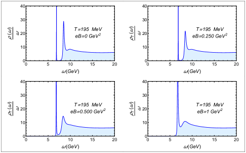
Figure 5: Spectral functions for bottomonium at T= 195 MeV for different values of a magnetic field perpendicular to the polarization

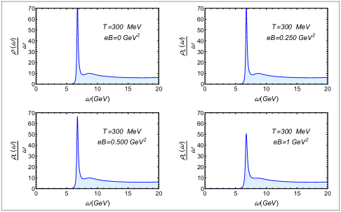
Figure 6: Spectral functions for bottomonium at T= 300 MeV for different values of a magnetic field parallel to the polarization

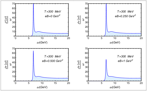
Figure 7: Spectral functions for bottomonium at T= 300 MeV for different values of a magnetic field perpendicular to the polarization

V Results and Discussion

The spectral functions for heavy vector mesons with polarization parallel (perpendicular) to the magnetic field are obtained evaluating numerically equations (40) (respectively (41)), with the boundary conditions (42) described in the previous section. The parameters used are the ones that provide the best fit in the zero temperature case of section II namely those of eq. (9) for charmonium and those of eq. (10) for bottomonium.

In order to have a clear picture of the thermal behavior of the spectra when there is no magnetic field, we show in figure 1 the charmonium and bottomonium spectra at four representative temperatures. One notes that for charmonium (left panel) there is a peak at $T=195$ MeV corresponding to the $1S$ state, the $J/\Psi$. At higher temperatures the peak decreases showing the dissociation process. For bottomonium there are two peaks at $T=195$ MeV. As the temperature increases the second state is strongly dissociated while the $1S$ state has a much smaller dissociation effect, compared with charmonium.

Then we show in figures 2 and 3 the cases of charmonium at a temperature of 195 MeV for magnetic fields parallel and perpendicular, respectively, to the polarization. This figures show that the dissociation effect increases with the magnetic field in both cases. When the magnetic field is perpendicular to the polarization of the meson the decrease in the spectral function peak is more noticeable then in the parallel case.

Figures 4 and 5 show the cases of bottomonium at $T=195$ MeV for magnetic fields parallel and perpendicular, respectively, to the polarization. One notes the clear dissociation of the second state as the effect of increasing magnetic fields. The cases of bottomonium at $T=300$ MeV are then presented in figures 6 and 7. The height of the peak of the first state, the $\Upsilon$, decreases as the magnetic field increases. As it happens with charmonium the dissociation effect produced by the magnetic field is stronger when it is perpendicular to the polarization direction.

The results provided by the model when there is no magnetic field are consistent with results for quarkonium dissociation temperatures using lattice QCD, potential models and other studies as presented in Adare:2014hje . For the case with magnetic field, there is a study, only for charmonium, using a holographic model in ref. Dudal:2014jfa . The main result found there is that for magnetic fields perpendicular to the polarization the dissociation is stronger than without the field, while for $eB$ fields parallel to the polarization the dissociation is weaker than without the field. Our result is different. In the presence of magnetic fields heavy vector mesons dissociate faster than without the field. The dissociation being faster for fields perpendicular to the polarization than for parallel fields.

It is important to stress the fact that our model, in contrast to ref. Dudal:2014jfa , reproduces the behavior of the decay constants obtained experimentally. As explained in the introduction, this is very important in order to find a consistent description of the thermal behavior.

Acknowledgments: N.B. is partially supported by CNPq (Brazil) under Grant No. 307641/2015-5 and L.F. is supported by CAPES (Brazil)

References

- (1) N. R. F. Braga, M. A. Martin Contreras and S. Diles, Eur. Phys. J. C 76, no. 11, 598 (2016) doi:10.1140/epjc/s10052-016-4447-4 [arXiv:1604.08296 [hep-ph]].
- (2) N. R. F. Braga and L. F. Ferreira, Phys. Lett. B 773, 313 (2017) doi:10.1016/j.physletb.2017.08.037 [arXiv:1704.05038 [hep-ph]].
- (3) N. R. F. Braga, L. F. Ferreira and A. Vega, Phys. Lett. B 774, 476 (2017) doi:10.1016/j.physletb.2017.10.013 [arXiv:1709.05326 [hep-ph]].
- (4) J. M. Maldacena, Adv. Theor. Math. Phys. 2, 231 (1998) [Int. J. Theor. Phys. 38, 1113 (1999)]. [arXiv:hep-th/9711200].
- (5) S. S. Gubser, I. R. Klebanov and A. M. Polyakov, Phys. Lett. B 428, 105 (1998). [arXiv:hep-th/9802109].
- (6) E. Witten, Adv. Theor. Math. Phys. 2, 253 (1998). [arXiv:hep-th/9802150].
- (7) J. Polchinski and M. J. Strassler, Phys. Rev. Lett. 88, 031601 (2002) [arXiv:hep-th/0109174].
- (8) H. Boschi-Filho and N. R. F. Braga, Eur. Phys. J. C 32, 529 (2004) [arXiv:hep-th/0209080].
- (9) H. Boschi-Filho and N. R. F. Braga, JHEP 0305, 009 (2003) [arXiv:hep-th/0212207].
- (10) A. Karch, E. Katz, D. T. Son and M. A. Stephanov, Phys. Rev. D 74, 015005 (2006) doi:10.1103/PhysRevD.74.015005 [hep-ph/0602229].
- (11) T. Sakai and S. Sugimoto, Prog. Theor. Phys. 113, 843 (2005) doi:10.1143/PTP.113.843 [hep-th/0412141].
- (12) N. R. F. Braga, M. A. Martin Contreras and S. Diles, Phys. Lett. B 763, 203 (2016) doi:10.1016/j.physletb.2016.10.046 [arXiv:1507.04708 [hep-th]].
- (13) T. Matsui and H. Satz, Phys. Lett. B 178, 416 (1986). doi:10.1016/0370-2693(86)91404-8.
- (14) H. Satz, J. Phys. G 32, R25 (2006) doi:10.1088/0954-3899/32/3/R01 [hep-ph/0512217].
- (15) D. E. Kharzeev, L. D. McLerran and H. J. Warringa, Nucl. Phys. A 803, 227 (2008) doi:10.1016/j.nuclphysa.2008.02.298 [arXiv:0711.0950 [hep-ph]].
- (16) K. Fukushima, D. E. Kharzeev and H. J. Warringa, Phys. Rev. D 78, 074033 (2008) doi:10.1103/PhysRevD.78.074033 [arXiv:0808.3382 [hep-ph]].
- (17) V. Skokov, A. Y. Illarionov and V. Toneev, Int. J. Mod. Phys. A 24, 5925 (2009) doi:10.1142/S0217751X09047570 [arXiv:0907.1396 [nucl-th]].
- (18) G. S. Bali, F. Bruckmann, G. Endrodi, Z. Fodor, S. D. Katz, S. Krieg, A. Schafer and K. K. Szabo, JHEP 1202, 044 (2012) doi:10.1007/JHEP02(2012)044 [arXiv:1111.4956 [hep-lat]].
- (19) E. S. Fraga and L. F. Palhares, Phys. Rev. D 86, 016008 (2012) doi:10.1103/PhysRevD.86.016008 [arXiv:1201.5881 [hep-ph]].
- (20) A. Ballon-Bayona, JHEP 1311, 168 (2013) doi:10.1007/JHEP11(2013)168 [arXiv:1307.6498 [hep-th]].
- (21) K. A. Mamo, JHEP 1505, 121 (2015) doi:10.1007/JHEP05(2015)121 [arXiv:1501.03262 [hep-th]].
- (22) D. Dudal, D. R. Granado and T. G. Mertens, Phys. Rev. D 93, no. 12, 125004 (2016) doi:10.1103/PhysRevD.93.125004 [arXiv:1511.04042 [hep-th]].
- (23) N. Evans, C. Miller and M. Scott, Phys. Rev. D 94, no. 7, 074034 (2016) doi:10.1103/PhysRevD.94.074034 [arXiv:1604.06307 [hep-ph]].
- (24) D. Li, M. Huang, Y. Yang and P. H. Yuan, JHEP 1702, 030 (2017) doi:10.1007/JHEP02(2017)030 [arXiv:1610.04618 [hep-th]].
- (25) A. Ballon-Bayona, M. Ihl, J. P. Shock and D. Zoakos, JHEP 1710, 038 (2017) doi:10.1007/JHEP10(2017)038 [arXiv:1706.05977 [hep-th]].
- (26) D. M. Rodrigues, E. Folco Capossoli and H. Boschi-Filho, arXiv:1709.09258 [hep-th].
- (27) K. A. Olive et al. [Particle Data Group Collaboration], Chin. Phys. C 38, 090001 (2014).
- (28) E. D’Hoker and P. Kraus, JHEP 0910, 088 (2009) doi:10.1088/1126-6708/2009/10/088 [arXiv:0908.3875 [hep-th]].
- (29) E. D’Hoker and P. Kraus, JHEP 1003, 095 (2010) doi:10.1007/JHEP03(2010)095 [arXiv:0911.4518 [hep-th]].
- (30) N. Iqbal and H. Liu, Phys. Rev. D 79, 025023 (2009) doi:10.1103/PhysRevD.79.025023 [arXiv:0809.3808 [hep-th]].
- (31) S. I. Finazzo, “Understanding strongly coupled non-Abelian plasmas using the gauge/gravity duality,” Phd Thesis, Universidade de São Paulo, 2015, DOI 10.11606/T.43.2015.tde-07042015-144444 .
- (32) A. Rebhan and D. Steineder, Phys. Rev. Lett. 108, 021601 (2012) doi:10.1103/PhysRevLett.108.021601 [arXiv:1110.6825 [hep-th]].
- (33) A. Adare et al. [PHENIX Collaboration], Phys. Rev. C 91, no. 2, 024913 (2015) doi:10.1103/PhysRevC.91.024913 [arXiv:1404.2246 [nucl-ex]].
- (34) D. Dudal and T. G. Mertens, Phys. Rev. D 91, 086002 (2015) doi:10.1103/PhysRevD.91.086002 [arXiv:1410.3297 [hep-th]].