A Deep Reinforcement Learning Based Approach
for Cost- and Energy-Aware Multi-Flow Mobile Data Offloading

Abstract

With the rapid increase in demand for mobile data, mobile network operators are trying to expand wireless network capacity by deploying wireless local area network (LAN) hotspots on to which they can offload their mobile traffic. However, these network-centric methods usually do not fulfill the interests of mobile users (MUs). Taking into consideration many issues such as different applications’ deadlines, monetary cost and energy consumption, how the MU decides whether to offload their traffic to a complementary wireless LAN is an important issue. Previous studies assume the MU’s mobility pattern is known in advance, which is not always true. In this paper, we study the MU’s policy to minimize his monetary cost and energy consumption without known MU mobility pattern. We propose to use a kind of reinforcement learning technique called deep Q-network (DQN) for MU to learn the optimal offloading policy from past experiences. In the proposed DQN based offloading algorithm, MU’s mobility pattern is no longer needed. Furthermore, MU’s state of remaining data is directly fed into the convolution neural network in DQN without discretization. Therefore, not only does the discretization error present in previous work disappear, but also it makes the proposed algorithm has the ability to generalize the past experiences, which is especially effective when the number of states is large. Extensive simulations are conducted to validate our proposed offloading algorithms.

1 Introduction

The mobile data traffic demand is growing rapidly. According to the investigation of Cisco Systems [1], the mobile data traffic is expected to reach 24.3 exabytes per month by 2019, while it was only 2.5 exabytes per month at the end of 2014. On the other hand, the growth rate of the mobile network capacity is far from satisfying that kind of the demand, which has become a major problem for wireless mobile network operators (MNOs). Even though 5G technology is promising for providing huge wireless network capacity [2], the development process is long and the cost is high. Economic methods such as time-dependent pricing [3][4] have been proposed to change users’ usage pattern, which are not user-friendly. Up to now, the best practice for increasing mobile network capacity is to deploy complementary networks (such as wireless LAN and femtocells), which can be quickly deployed and is cost-efficient. Using such methods, part of the MUs’ traffic demand can be offloaded from a MNO’s cellular network to the complementary network.
The process that a mobile device automatically changes its connection type (such as from cellular network to wireless LAN) is called vertical handover [5]. Mobile data offloading is facilitated by new standards such as Hotspot 2.0 [6] and the 3GPP Access Network Discovery and Selection Function (ANDSF) standard [7], with which information of network (such as price and network load) can be broadcasted to MUs in real-time. Then MUs can make offloading decisions intelligently based on the real-time network information.
There are many works related to the wireless LAN offloading problem. However, previous works either considered the wireless LAN offloading problem from the network providers’ perspective without considering the MU’s quality of service (QoS) [8][9], or studied wireless LAN offloading from the MU’s perspective [10][11] [12][13], but without taking the energy consumption as well as cost problems into consideration.
[14][15] studied wireless LAN offloading problem from MU’s perspective. While single-flow mobile date offloading was considered in [14], multi-flow mobile data offloading problem is studied in [15] in which a MU has multiple applications to transmit data simultaneously with different deadlines. MU’s target was to minimize its total cost, while taking monetary cost, preference for energy consumption, application’s delay tolerance into consideration. This was formulated the wireless LAN offloading problem as a finite-horizon discrete-time Markov decision process [16][17][18]. A high time complexity dynamic programming (DP) based optimal offloading algorithm and a low time complexity heuristic offloading algorithm were prosed in [15].

TABLE I: Comparison of different works.

References	Multi-flow	Unknown mobility pattern	No discretization error	Energy consideration	Q-value prediction
[13]	$\times$	$\times$	$\times$	$\times$	—
[14]	$\times$	$\checkmark$	$\times$	$\checkmark$	$\times$
[15]	$\checkmark$	$\times$	$\times$	$\checkmark$	—
This paper	$\checkmark$	$\checkmark$	$\checkmark$	$\checkmark$	$\checkmark$

One assumption in [15] was that MU’s mobile pattern from one place to another is known in advance, then the transition probability, which is necessary for optimal policy calculation in MDP, can be obtained in advance. However, the MU’s mobility pattern may not be easily obtained or the accuracy is not high. Even though a Q-learning [19] based algorithm was proposed in [14] for the unknown MU’s mobility pattern case, the learning, the convergence rate of the proposed algorithm is rather low due to the large number of states. It takes time for the reinforcement learning agent to experience all the states to estimate the Q-value.
In this paper, we propose a deep reinforcement learning algorithm, specifically, a deep Q-network (DQN) [20] based algorithm, to solve the multi-flow offloading problem with high convergence rate without knowing MU’s mobility pattern. In reinforcement learning, the agent learns to make optimal decisions from past experience when interacting with the environment (see Fig. 1). In the beginning, the agent has no knowledge of the task and makes decision (or takes action), then, it receives a reward based on how well the task is done. Theoretically, if the agent experience all the situations (states) and get to know the value of its decision on all situations, the agent can make optimal decisions. However, often it is impossible for the agent to experience all situations. The agent does not have the ability to generalize its experience when unknown situations appear. Therefore, DQN [20] was developed to let agent generalize its experience. DQN uses deep neural networks (DNN) [21] to predict the Q-value in standard Q-learning, which is a value that maps from agent’s state to different actions. Then, the optimal offload action can be directly obtained by choosing the one that has the maximum Q-value. Please refer to Table. I for the comparison of different works.
The rest of this paper is organized as follows. Section 2 illustrates the system model. Section 3 defines MU’s mobile data offloading optimization target. Section 4 proposes DQN based algorithm. Section 5 illustrates the simulation and results. Finally, we conclude this paper in Section 6.

2 System Model

Since the cellular network coverage is rather high, we assume the MU can always access the cellular network, but cannot always access wireless LAN. The wireless LAN access points (APs) are usually deployed at home, stations, shopping malls and so on. Therefore, we assume that wireless LAN access is location-dependent. We mainly focus on applications with data of relative large size and delay-tolerance to download, for example, applications like software updates, file downloads. The MU has $M$ files to download from a remote server. Each file forms a flow, and the set of flows is denoted as $\mathcal{M}$$=$$\{1,...,M\}$. Each flow $j\in\mathcal{M}$ has a deadline $T^{j}$. T$=$$(T^{1},T^{2},...,T^{M})$ is the deadline vector for the MU’s $M$ flows. Without loss of generality, it is assumed that $T^{1}\leq T^{2}\leq...\leq T^{M}$. We consider a slotted time system as $t$$\in$$\mathcal{T}$$=$$\{1,...,T^{M}\}$.

We only considered delay-tolerant traffic in this paper in which $T^{j}>0$ for $j\in\mathcal{M}$. For non-delay-tolerant traffic, the deadline $T^{j}=0$. In this case, MU has to start to transmit data whenever there is a network available without network selection.

To simplify the analysis, we use limited discrete locations instead of infinite continuous locations. It is assumed that a MU can move among the $L$ possible locations, which is denoted as set $\mathcal{L}$$=$$\{1,...,L\}$. While the cellular network is available at all the locations, the availability of wireless LAN network is dependent on location $l\in\mathcal{L}$. The MU has to make a decision on what network to select and how to allocate the available data rate among $M$ flows at location $l$ at time $t$ by considering total monetary cost, energy consumption and remaining time for data transmission. The consideration of MU’s energy consumption is one feature of our series of works [14][15]. When the data rate of wireless LAN is too low, the energy consumption per Mega bytes data is high [22] (see Fig.2 ) and it will take a long time to transmit MU’s data. For MUs who care about energy consumption or have a short deadline for data transmission, they may choose to use cellular network with high data rate even if wireless LAN is available. As in [13][14][15] the MU’s decision making problem can be modeled as a finite-horizon Markov decision process.

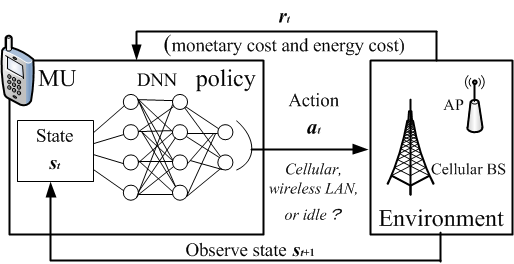
Figure 1: An deep Q-network based modeling: at time decision epoch $t$, the state of MU contains location $l$ and remaining file size B, which is fed into a deep neural network to generate optimal policy. Then MU chooses actions of Wireless LAN, Cellular network, or Idle, which incur different cost on MU. The objective of MU is to minimize total cost from time $1$ to $T$.

We define the system state at $t$ as in Eq. (1)

$$\textbf{{s}}_{t}=\{l_{t},\textbf{{b}}_{t}\}$$ (1)

where $l_{t}\in\mathcal{L}$$=$$\{1,...,L\}$ is the MU’s location index at time $t$, which can be obtained from GPS. $\mathcal{L}$ is the location set. $\textbf{{b}}_{t}$$=$$(b_{t}^{1},b_{t}^{2},...,b_{t}^{M})$ is the vector of remaining file sizes of all $M$ flows at time $t$, $b_{t}^{j}\in\mathcal{B}^{j}$ $=[0,B^{j}]$ for all $j\in\mathcal{M}$. $B^{j}$ is the total file size to be transmitted on flow $j$. $b_{t}^{j}$ is equal to $B^{j}$ before flow $j$ starts to transmit. $\mathcal{B}$=$(\mathcal{B}^{1},\mathcal{B}^{2},...,\mathcal{B}^{M})$ is the set of vectors.
The MU’s action $a_{t}$ at each decision epoch $t$ is to determine whether to transmit data through wireless LAN (if wireless LAN is available), or cellular network, or just keep idle and how to allocate the network data rate to $M$ flows. Please note that epoch is the same as time slot, at which MU makes action decision. We use epoch and time slot interchangeably in this paper. The reason why MU does not choose any of the network is that MU may try to wait for free or low price wireless LAN to save his/her money even though cellular is ready anytime. The survey in [23] had the results that more than 50% of the respondents would like to wait for 10 minutes to stream YouTube videos and 3-5 hours to download a file a if monetary incentive is given. The reason why MU does not choose any of the network is that MU may try to wait for free or low price wireless LAN to save his/her money even though cellular is ready anytime. The survey in [23] had the results that more than 50% of the respondents would like to wait for 10 minutes to stream YouTube videos and 3-5 hours to download a file a if monetary incentive is given.

Therefore, the MU’s action vector is denoted as in Eq. (2)

$$\textbf{{a}}_{t}=(\textbf{{a}}_{t,c},\textbf{{a}}_{t,w})$$ (2)

where $\textbf{{a}}_{t,c}=(a_{t,c}^{1},a_{t,c}^{2},...,a_{t,c}^{M})$ denotes the vector of cellular network allocated data rates, $a_{t,c}^{j}$ denotes the cellular data rate allocated to flow $j\in$$\mathcal{M}$, and $\textbf{{a}}_{t,w}=(a_{t,w}^{1},a_{t,w}^{2},...,a_{t,w}^{M})$ denotes the vector of wireless LAN network allocated data rates, and $a_{t,w}^{j}$ denotes the wireless LAN rate allocated to flow $j\in$$\mathcal{M}$. Here the subscript $c$ and $w$ stand for cellular network and wireless LAN, respectively. Please note that $a_{t,w}^{1}$, $a_{t,w}^{2}$, …, $a_{t,w}^{M}$ all can be 0 if the MU is not in the coverage area of wireless LAN AP. Even though it is technically possible that wireless LAN and cellular network can be used at the same time, we assume that the MU can not use wireless LAN and cellular network at the same time. We make this assumption for two reasons: (i) If we restrict the MU to use only one network interface at the same time slot, then the MU’s device may be used for longer time with the same amount of left battery. (ii) Nowadays smartphones, such as an iPhone, can only use one network interface at the same time. We can easily implement our algorithms on a MU’s device without changing the hardware or OS of the smartphone if we have this assumption. At time $t$, MU may choose to use wireless LAN (if wireless LAN is available) or cellular network, or not to use any network. If the MU chooses wireless LAN at $t$, the wireless LAN network allocated data rate to flow $j$, $a_{t,w}^{j}$, is greater than or equal to 0, and the MU does not use cellular network in this case, then $a_{t,c}^{j}$ = 0. On the other hand, if the MU chooses cellular network at $t$, the cellular network allocated data rate to flow $j$, $a_{t,c}^{j}$, is greater than or equal to 0, and the MU does not use wireless LAN in this case, then $a_{t,w}^{j}$ = 0. $a_{t,n}^{j}$, $n\in\{c,w\}$ should not be greater than the remaining file size $b_{t}^{j}$ for flow $j\in$$\mathcal{M}$.
The sum data rate of all the flows of cellular network and wireless LAN are denoted as $a_{t,c}=\sum_{j\in\mathcal{M}}a_{t,c}^{j}$ and $a_{t,w}=\sum_{j\in\mathcal{M}}a_{t,w}^{j}$, respectively. $a_{t,c}$ and $a_{t,w}$ should satisfy the following conditions.

$$a_{t,c}\leq\gamma_{c}^{l}$$ (3)

$$a_{t,w}\leq\gamma_{w}^{l}$$ (4)

$\gamma_{c}^{l}$ and $\gamma_{w}^{l}$ are the maximum data rates of cellular network and wireless LAN, respectively, at each location $l$.

TABLE II: Notations summary.

Notation	Description
$\mathcal{M}$	$\mathcal{M}$$=$$\{1,...,M\}$, MU’s $M$ flows set.
T	T$=$$(T^{1},T^{2},...,T^{M})$, MU’s deadline vector.
$t$	$t\in\mathcal{T}^{M}$, the specific decision epoch of MU.
$\mathcal{L}$	$\mathcal{L}$$=$$\{1,...,L\}$, the location set of MU.
$\mathcal{B}^{j}$	$\mathcal{B}^{j}$$\subseteq$$[0,...,b_{t}^{j}]$, the total size of MU’s $j$ flow. $j\in\mathcal{M}$.
$\textbf{{b}}_{t}$	$\textbf{{b}}_{t}$$=$$(b_{t}^{1},b_{t}^{2},...,b_{t}^{M})$, vector of remaining file size.
$\textbf{{s}}_{t}$	$\textbf{{s}}_{t}=(l_{t},\textbf{{b}}_{t})$, state of MU.
$l_{t}$	$l_{t}\in\mathcal{L}$, MU’s location index at time $t$.
$a_{t,c}^{j}$	cellular data rate allocated to flow $j\in$$\mathcal{M}$ at time $t$
$a_{t,w}^{j}$	wireless LAN data rate allocated to flow $j\in$$\mathcal{M}$ at time $t$
$\textbf{{a}}_{t,c}$	$\textbf{{a}}_{t,c}=\{a_{t,c}^{1},a_{t,c}^{2},...,a_{t,c}^{M}\}$
$\textbf{{a}}_{t,w}$	$\textbf{{a}}_{t,w}=\{a_{t,w}^{1},a_{t,w}^{2},...,a_{t,w}^{M}\}$
$\textbf{{a}}_{t}$	$\textbf{{a}}_{t}=(\textbf{{a}}_{t,c},\textbf{{a}}_{t,w})$
$a_{t,c}$	$a_{t,c}=\sum_{j\in\mathcal{M}}a_{t,c}^{j}$
$a_{t,w}$	$a_{t,w}=\sum_{j\in\mathcal{M}}a_{t,w}^{j}$
$\gamma_{c}^{l}$	cellular throughput in bps at location $l$.
$\gamma_{w}^{l}$	wireless LAN throughput in bps at location $l$.
$\varepsilon_{c}^{l}$	energy consumption rate of celllar network in joule/bits at location $l$.
$\varepsilon_{w}^{l}$	energy consumption rate of wireless LAN in joule/bits at location $l$.
$\theta_{t}$	energy preference of MU at $t$.
$p_{c}$	MNO’s usage-based price for cellular network service.
$\hat{c}_{T^{M}+1}(\cdot)$	MU’s penalty function for remaining data at $T^{M}+1$.
$\xi_{t}(\textbf{{s}}_{t},\textbf{{a}}_{t})$	MU’s energy consumption at $t$.
$\phi_{t}$	$\mathcal{L}$$\times$$\mathcal{K}$$\rightarrow$$\mathcal{A}$, transmission decision at $t$.
$\pi$	$\pi=\{\phi_{t}(l,b),\;\forall\;t\in\mathcal{T^{M}},l\in\mathcal{L},b\in\mathcal{B}\}$, MU’s policy.

At each epoch $t$, three factors affect the MU’s decision.

(1) monetary cost: it is the payment from the MU to the network service provider. We assume that the network service provider adopts usage-based pricing, which is being widely used by carriers in Japan, USA, etc. The MNO’s price is denoted as $p_{c}$. It is assumed that wireless LAN is free of charge. We define the monetary cost $c_{t}(\textbf{{s}}_{t},\textbf{{a}}_{t})$ as in Eq. (5)

$$c_{t}(\textbf{{s}}_{t},\textbf{{a}}_{t})=p_{c}\sum_{j\in\mathcal{M}}\min\{b_{t}^{j},\delta a_{t,c}^{j}\}$$ (5)

(2) energy consumption: it is the energy consumed when transmitting data through wireless LAN or cellular network. We denote the MU’s awareness of energy as in Eq. (6)

$$\begin{split}\xi_{t}(\textbf{{s}}_{t},\textbf{{a}}_{t})=&\theta_{t}(\varepsilon_{c}^{l}\sum_{j\in\mathcal{M}}\min\{b_{t}^{j},\delta a_{t,c}^{j}\}\\ &+\varepsilon_{w}^{l}\sum_{j\in\mathcal{M}}\min\{b_{t}^{j},\delta a_{t,w}^{j}\})\end{split}$$ (6)

where $\varepsilon_{c}^{l}$ is the energy consumption rate of the cellular network in joule/bits at location $l$ and $\varepsilon_{w}^{l}$ is the energy consumption rate of the wireless LAN in joule/bits at location $l$. It has been shown in [24] that both $\varepsilon_{c}^{l}$ and $\varepsilon_{w}^{l}$ decrease with throughput, which means that low transmission speed consumes more energy when transmitting the same amount of data. According to [25], the energy consumptions for downlink and uplink are different. Therefore, the energy consumption parameters $\varepsilon_{c}^{l}$ and $\varepsilon_{w}^{l}$ should be differentiated for downlink or uplink, respectively. In this paper, we do not differentiate the parameters for downlink or uplink because only the downlink case is considered. Nevertheless, our proposed algorithms are also applicable for uplink scenarios with energy consumption parameters for uplink. $\theta_{t}$ is the MU’s preference for energy consumption at time $t$. $\theta_{t}$ is the weight on energy consumption set by the MU. Small $\theta_{t}$ means that the MU cares less on energy consumption. For example, if the MU can soon charge his smartphone, he may set $\theta_{t}$ to a small value, or if the MU is in an urgent status and could not charge within a short time, he may set a large value for $\theta_{t}$. $\theta_{t}$ = 0 means that the MU does not consider energy consumption during the data offloading

(3) penalty: if the data transmission does not finish before deadline $T^{j}$, $j\in\mathcal{M}$, the penalty for the MU is defined as Eq. (7).

$$\hat{c}_{T^{j}+1}(\textbf{{s}}_{T^{j}+1})=\hat{c}_{T^{j}+1}(l_{T^{j}+1},\textbf{{b}}_{T^{j}+1})=g(\textbf{{b}}_{T^{j}+1})$$ (7)

where $g(\cdot)$ is a non-negative non-decreasing function. ${T^{j}+1}$ means that the penalty is calculated after deadline $T^{j}$.

3 Problem Formulation

MU has to decide all the actions from the first time epoch to the last one to minimize overall monetary cost and energy consumption for all the time epochs. Policy is the sequence of actions from the first time epoch to the last one. We formally have definition for policy as follows.

Definition 1

The MU’s policy is the actions he takes from from $t=1$ to $t=T^{M}$, which is defined as in Eq. (8)

$$\pi=\bigg{\{}\phi_{t}(l_{t},\textbf{{b}}_{t}),\;\forall\;t\in\mathcal{T},l\in\mathcal{L},\textbf{{b}}_{t}\in\mathcal{B}\bigg{\}}$$ (8)

where $\phi_{t}(l_{t},\textbf{{b}}_{t})$ is a function mapping from state $\textbf{{s}}_{t}=(l_{t},\textbf{{b}}_{t})$ to a decision action at $t$.

The set of $\pi$ is denoted as $\Pi$. If policy $\pi$ is adopted, the state is denoted as $\textbf{{s}}_{t}^{\pi}$.

The objective of the MU is to the minimize the expected total cost (include the monetary cost and the energy consumption) from $t=1$ to $t=T^{M}$ and penalty at $t=$${T^{M}+1}$ with an a optimal $\pi^{*}$ (see Eq. (9))

$$\min_{\pi\in\Pi}E_{\textbf{{s}}_{1}}^{\pi}\Bigg{[}\sum_{t=1}^{T^{M}}r_{t}(\textbf{{s}}_{t}^{\pi},\textbf{{a}}_{t})+\sum_{j\in\mathcal{M}}\hat{c}_{T^{j}+1}(\textbf{{s}}_{T^{j}+1}^{\pi})\Bigg{]}$$ (9)

where $r_{t}(\textbf{{s}}_{t},\textbf{{a}}_{t})$ is the sum of the monetary cost and the energy consumption as in Eq. (10)

$$r_{t}(\textbf{{s}}_{t},\textbf{{a}}_{t})=c_{t}(\textbf{{s}}_{t},\textbf{{a}}_{t})+\xi_{t}(\textbf{{s}}_{t},\textbf{{a}}_{t})$$ (10)

The optimal policy is the the optimal solution of the minimization problem defined in Eq. (9). Please note that the optimal action at each $t$ does not lead to the optimal solution for the problem in Eq. (9). At each time $t$, not only the cost for the current time $t$ should be considered, but also the future expected cost.
The objective function of the minimization problem Eq.(9) includes three parts. The first two parts are denoted in $r_{t}(\textbf{{s}}_{t},\textbf{{a}}_{t})$, which contains monetary cost and energy consumption. As shown in Eq. (5), the monetary cost is determined by the cellular network price $p_{c}$ and the data transmitted through cellular network $a_{t,c}^{j}$. The parameter $a_{t,c}^{j}$ is the one that MU tries to determine in each time epoch $t$, which has the priority all the time. On the other hand, as shown in the Eq. (6), the parameters to minimize for energy consumption are $a_{t,c}^{j}$ and $a_{t,w}^{j}$, which are the data transmitted through cellular network and wireless LAN, respectively. Whether the energy consumption has priority is determined by the MU’s preference parameter $\theta_{t}$. Obviously, if $\theta_{t}$ is set to zero by MU, Eq. (6) become zero and there is no priority for energy consumption in the target minimization problem. In this case, the value the minimization in Eq. (9) reached is the minimized total monetary cost. If $\theta_{t}$ is set to nonzero by MU, Eq. (6) is also nonzero and energy consumption is also incorporated in the target minimization problem. In this case, the value the minimization in Eq. (9) reached is the minimized total monetary cost and energy consumption. The third part is the penalty defined in Eq. (7). The remaining data after deadline determines the penalty, which can not be directly controlled by MU. MU can only try to finish the data transmission before the deadline to eliminate the penalty.

4 DQN Based Offloading Algorithm

In reinforcement learning, an agent makes optimal decision by acquiring knowledge of the unknown environment through reinforcement. In our model in this paper, MU is the agent. The state is the location and remaining data size. The action is to choose cellular network, wireless LAN, or none of the two. The negative reward is the monetary cost and energy consumption at each time epoch. The MU’s goal is to minimize the total monetary cost and energy consumption over all the time epochs.

One important difference that arises in reinforcement learning and not in other kinds of learning is the trade-off between exploration and exploitation. To minimize the total monetary cost and energy consumption, MU must prefer actions that it has tried in the past and found to be effective in reducing monetary cost and energy consumption. But to discover such actions, it has to try actions that it has not selected before. The MU has to exploit what it already knows in order to reduce monetary cost and energy consumption, but it also has to explore in order to make better action selections in the future.

Initially, the MU has no experience. The MU has to explore unknown actions to get experience of monetary cost and energy consumption for some states. Once it gets the experiences, it can exploit what it already knows for the states but keep exploring at the same time. We use the parameter $\epsilon$ in Algorithm 1 to set the trade-off between exploration and exploitation.

There are many methods for MU to get optimal policy in reinforcement learning. Our previous work [14] adopted a Q-learning based approach, which is a kind of temporal difference (TD) learning algorithm [19]. TD learning algorithms require no model for the environment and are fully incremental. The core idea of Q-learning is to learn an action-value function that ultimately gives the expected MU’s cost of taking a given action in a given state and following the optimal policy thereafter. The optimal action-value function follows the following optimality equation (or Bellman equation) in Eq. (11) [26].

$$\mathcal{Q}_{t}^{*}(\textbf{{s}}_{t},\textbf{{a}}_{t})=\mathbb{E}_{\textbf{{s}}_{t+1}}\big{[}r_{t}(\textbf{{s}}_{t},\textbf{{a}}_{t})+\gamma\min_{\textbf{{a}}_{t+1}}\mathcal{Q}_{t}(\textbf{{s}}_{t+1},\textbf{{a}}_{t+1})|\textbf{{s}}_{t},\textbf{{a}}_{t}\big{]}$$ (11)

where $\gamma$ is the discount factor in (0,1). The value of the action-value function is called Q-value. In Q-learning algorithm, the optimal policy can be easily obtained from optimal Q-value, $\mathcal{Q}_{t}^{*}(\textbf{{s}},a)$, which is shown in Eq. (12)

$$\phi_{t}^{*}=\arg\min_{\textbf{{a}}_{t}\in\mathcal{A}}\mathcal{Q}_{t}^{*}(\textbf{{s}}_{t},\textbf{{a}}_{t})$$ (12)

Transition probability (or MU’s mobility pattern, please note that when we mention ”unknown transition probability” in this paper, it is also means ”unknown mobility pattern”) that is necessary in [15] is no longer needed in Q-learning based offloading algorithm. However, there are three problems in the reinforcement learning algorithm in [14].

	Algorithm 1: DQN Based Offloading Algorithm
1:	Initialize replay memory $D$ to capacity $N$
2:	Initialize action-value function $\mathcal{Q}$ with random parameters $\theta$
3:	Initialize target action-value function $\bar{\mathcal{Q}}$ with parameters $\theta^{-}$
4:	Set $t:=1$, $\textbf{{b}}_{1}:=\mathcal{B}$, and set $l_{1}$ randomly.
5:	Set $\textbf{{s}}_{1}=(l_{1},\textbf{{b}}_{1})$
6:	while $t\leq T$ and $b>0$:
7:	$l_{t}$ is determined from GPS
8:	$rnd$ $\leftarrow$ random number in [0,1]
9:	if $rnd$ $<$ $\epsilon$ :
10:	Choose action $a$ randomly
11:	else:
12:	Choose action $a$ based on Eq. (13)
13:	end if
14:	Set $\textbf{{s}}_{t+1}=(l_{t}\textbf{,}[\textbf{{b}}_{t}-\delta\textbf{{a}}_{t,c}-\delta\textbf{{a}}_{t,w}]^{+})$
15:	Calculate $r_{t}(\textbf{{s}}_{t},\textbf{{a}}_{t})$ by Eq. (10)
16:	Store experience $(\textbf{{s}}_{t},\textbf{{a}}_{t},r_{t},\textbf{{s}}_{t+1})$ in $D$
17:	Sample random minibatch of $(\textbf{{s}}_{j},\textbf{{a}}_{j},r_{j},\textbf{{s}}_{j+1})$ from $D$
18:	if $j+1$ is termination:
19:	Set $z_{j}$ = $r_{j}$
20:	else:
21:	Set $z_{j}$ = $r_{j}+\gamma\min_{\textbf{{a}}_{j+1}}\mathcal{Q}_{t}(\textbf{{s}}_{j+1},\textbf{{a}}_{j+1};\theta_{j}^{-})$
22:	end if
23:	Execute a gradient descent step on $(z_{j}-\mathcal{Q}_{t}(\textbf{{s}}_{t},\textbf{{a}}_{t};\theta)^{2}$ with respect to parameters $\theta$.
24:	Every C steps reset $\mathcal{\bar{Q}}$=$\mathcal{Q}$
25:	Set $t:=t+1$
26:	end while

• (i) The state discretization induces error. The state of remaining data is continuous, which is discretized in algorithms in [14] and [15] as well. One way to reduce the error is to use small granularity to discretize the remaining data, which increases the number of state.

• (ii) The large number of state makes it difficult to implement the Q-learning algorithm. The simplest way of implementation is to use two-dimension table to store Q-value data, in which one of the dimensions indicates states and the other indicates actions. The method quickly becomes inviable with increasing sizes of state/action.

• (iii) The convergence rate of the algorithm is rather low. The algorithm begins to converge if MU experience many states and the agent does not have the ability to generalize its experience to unknown states.

Therefore, we propose to use DQN [20] based algorithm to solve the problem in Eq.(9). In DQN based algorithm, DNN [21] is used to generalize MU’s experience to predict the Q-value of unknown states. Furthermore, the continuous state of remaining data is fed into DNN directly without discretization error.

In DQN, the action-value function is estimated by a function approximator $\mathcal{Q}_{t}(\textbf{{s}},a;\mathbf{\theta})$ with parameters $\mathbf{\theta}$. Then MU’s optimal policy is obtained from the following Eq.(13) instead of Eq.(12)

$$\phi_{t}^{*}=\arg\min_{\textbf{{a}}_{t}\in\mathcal{A}}\mathcal{Q}_{t}^{*}(\textbf{{s}}_{t},\textbf{{a}}_{t};\theta)$$ (13)

A neural network function approximator with weights $\mathbf{\theta}$ is called as a Q-network. The Q-network can be trained by changing the parameters $\theta_{i}$ at iteration $i$ to decrease the mean-squared error in the Bellman equation, where the optimal target values in Eq.(11), $r_{t}(\textbf{{s}}_{t},\textbf{{a}}_{t})+\gamma\min_{\textbf{{a}}_{t+1}}\mathcal{Q}_{t}(\textbf{{s}}_{t+1},\textbf{{a}}_{t+1})$, are replaced by the approximate target values

$$z=r_{t}(\textbf{{s}}_{t},\textbf{{a}}_{t})+\gamma\min_{\textbf{{a}}_{t+1}}\mathcal{Q}_{t}(\textbf{{s}}_{t+1},\textbf{{a}}_{t+1};\theta_{i}^{-})$$ (14)

where $\theta_{i}^{-}$ is the parameter in the past iteration.

The mean-squared error (or loss function) is defined as in Eq.(15).

$$L_{i}(\theta_{i})=\mathbb{E}_{\textbf{{s}}_{t},\textbf{{a}}_{t},r_{t},\textbf{{s}}_{t+1}}\big{[}(z-\mathcal{Q}_{t}(\textbf{{s}}_{t},\textbf{{a}}_{t};\mathbf{\theta}_{i}))^{2}\big{]}$$ (15)

The gradient of loss function can be obtained by differentiation as follows.

$$\begin{split}&\nabla_{\theta_{i}}L_{i}(\theta_{i})=\\ &\mathbb{E}_{\textbf{{s}}_{t},\textbf{{a}}_{t},r_{t},\textbf{{s}}_{t+1}}\big{[}\big{(}z-\mathcal{Q}_{t}(\textbf{{s}}_{t},\textbf{{a}}_{t};\mathbf{\theta}_{i})\big{)}\nabla_{\theta_{i}}\mathcal{Q}_{t}(\textbf{{s}}_{t},\textbf{{a}}_{t};\mathbf{\theta}_{i})\big{]}\end{split}$$ (16)

The gradient $\nabla_{\theta_{i}}\mathcal{Q}_{t}(\textbf{{s}}_{t},\textbf{{a}}_{t};\mathbf{\theta}_{i})$ gives the direction to minimize the loss function in Eq.(15). The parameter are updated by the following rule in Eq.(17)

$$\theta_{i+1}=\theta_{i+1}+\alpha\nabla_{\theta_{i}}L_{i}(\theta_{i})$$ (17)

where $\alpha$ is the learning rate in (0,1). The proposed DQN based offloading algorithm is shown in Algorithm 1. As shown from line 16 to line 23 in Algorithm 1, MU’s experience $(\textbf{{s}}_{t},\textbf{{a}}_{t},r_{t},\textbf{{s}}_{t+1})$ are stored in replay memory. Therefore, transition probability is no longer needed. The Q-value is estimated from continuous state in line 21 without discretization. Therefore, there is no discretization error.

The mobile terminal has all the information needed in reinforcement learning: the state, action, monetary cost and energy consumption at each time $t$, and the goal. Specifically, the mobile terminal has the location information from GPS, and the keep recording the remaining data for each flow, then mobile terminal has the information of state. The mobile terminal can also detect the candidate actions–cellular network, wireless LAN–at each location at each time epoch. Since the price of cellular network and energy consumption for different data rate is already known by MU, then the monetary cost and energy consumption information are also known to MU. The server just provides data source for mobile terminal to download.

5 Performance Evaluation

In this section, the performances of our proposed DQN based offloading algorithm are evaluated by comparing them with dynamic programming based offloading algorithm (DP) and heuristic offloading (Heuristic) algorithm in our previous work [15]. We employed the DP and Heuristic methods as comparative methods to show that our proposed reinforcement learning based algorithm is effective even if the MU’s mobility pattern (or transition probability) from one place to another is unknown.

While the DP algorithm was proposed to get the optimal solution of the formulated Markov decision process (MDP) problem, the Heuristic algorithm was proposed to get near-optimal solution of the same problem with low time-complexity. These two algorithms were based on the assumption that MU’s transition probability from one place to another is known in advance. We try to show by comparison that our proposed DQN algorithm in this paper is valid even if the MU’s transition probability is unknown.

Since the transition probability is necessary for DP and heuristic algorithms to work, we input some ”incorrect” transition probability by adding some noise to the MU’s ”true” transition probability and check the performance.
We developed a simulator by Python 2.7, which can be downloaded from URL link (https://github.com/aqian2006/
OffloadingDQN).

TABLE III: Energy vs. Throughput.

Throughput (Mbps)	Energy (joule/Mb)
11.257	0.7107
16.529	0.484
21.433	0.3733

A four by four grid is used in simulation. Therefore, $L$ is 16. Wireless LAN APs are randomly deployed in $L$ locations. The cellular usage price is assumed as 1.5 yen/Mbyte. It is assumed that each location is a square of 10 meters by 10 meters. The MU is an pedestrian and the time slot length is assumed as 10 seconds. The epsilon greedy parameter $\epsilon$ is set to 0.08. $\textrm{Pr}(l|l)=0.6$ means that the probability that MU stays in the same place from time $t$ to $t^{\prime}$ is 0.6. And MU moves to the neighbour location with equal probability, which can be calculated as $\textrm{Pr}(l_{t+1}|l_{t})=(1-0.6)/(\textrm{number of neighbors})$. Because DP algorithm in [15] can not work without transition probability information, we utilize the aforementioned transition probability but add some noise to the transition probability. Please note that our proposed DQN based algorithm do not need the transition probability Pr. The Pr is externally given to formulate the simulation environment. The less the Pr is, the more dynamic of MU is. High Pr value means the the probability that MU stays a the same place is high. If Pr is changed to small value, the proposed DQN based algorithm is expected to have better performance. The reason is that in the DQN based algorithm, the exploration and exploitation is incorporated into the algorithm, which can adapt to environment changes. The average Wireless LAN throughput $\gamma_{t,w}^{l}$ is assumed as 15 Mbps, while average cellular network throughput $\gamma_{t,c}^{l}$ is 10 Mbps. We generate wireless LAN throughput for each AP from a truncated normal distribution, and the mean and standard deviation are assumed as 15Mbps and 6Mbps respectively. The wireless LAN throughput is in the range [9Mbps, 21Mbps]. Similarly, we generate cellular throughput from a truncated normal distribution, and the mean and standard deviation are assumed as 10Mbps and 5Mbps respectively. The cellular network throughput is in range [5Mbps, 15Mbps]. $\sigma$ in Algorithm 1 is assumed as 1 Mbytes. Each epoch lasts for 1 seconds. The penalty function is assumed as $g(\textbf{{b}}_{t})$=$2\sum_{j\in\mathcal{M}}b_{t}^{j}$. Please refer to Table IV for the parameters used in the simulation.

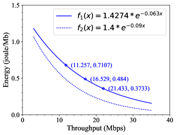
Figure 2: Energy consumption (joule/Mb) vs. Throughput (Mbps).

Because the energy consumption rate is a decreasing function of throughput, we have the sample data from [22] (see Table III). We then fit the sample data by an exponential function $f_{1}(x)=1.4274*\mathrm{e}^{-0.063x}$ as shown in Fig. 2. We also made a new energy-throughput function as $f_{2}(x)=1.4*\mathrm{e}^{-0.09x}$, which is just lower than $f_{1}(x)$. If we do not explicitly point that we use $f_{2}(x)$, we basically use $f_{1}(x)$. Please note that the energy consumption rate of cellular and wireless LAN may be different for the same throughput, but we assume they are the same and use the same fitting function as in Fig. 2.

TABLE IV: Parameters in the simulation.

Parameters	Value
$L$	16
B	$\textbf{{B}}=(400,600,800,1000)$ Mbytes
$\mathcal{T}$	$\mathcal{T}=(400,800,1200,1600)$
Number of wireless LAN APs	8
$\sigma$	1 Mbytes
time slot	10 seconds
$\epsilon$	0.08
average of $\gamma_{c}^{l}$	10 Mbps
standard deviation of $\gamma_{c}^{l}$	5 Mpbs
average of $\gamma_{w}^{l}$	15 Mbps
standard deviation of $\gamma_{w}^{l}$	6 Mpbs
$\textrm{Pr}({l|l})$	0.6
$\textrm{Pr}(l_{t+1}|l_{t})$	(1-0.6)/#neigbour locations
$p_{c}$	1.5 yen per Mbyte
$g(\textbf{{b}}_{t})$	$g(\textbf{{b}}_{t})$=$2\sum_{j\in\mathcal{M}}b_{t}^{j}$

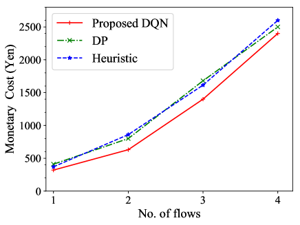
Figure 3: Monetary cost (yen) vs. No. of flows.

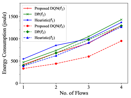
Figure 4: Energy consumption (joule) vs. No. of flows with different energy-throughput functions $f_{1}$ and $f_{2}$.

Fig.3 shows the comparison of monetary cost among Proposed DQN, Heuristic and DP algorithms with different number of flows. The monetary cost of all three algorithms increases with the number of flows. Please note that we fixed the number of APs to 8 in Table 4.

The monetary cost of Proposed DQN is lower than DP and Heuristic. And the Heuristic sometimes performance better than DP. The reason is that the DP algorithm with incorrect transition probability cannot obtain optimal policy, while our Proposed DQN can learn how to choose optimal policy with unknown transition probability.

Fig.4 shows the comparison of the energy consumption among Proposed DQN, Heuristic and DP algorithms with different number of flows. Two energy-throughput functions $f_{1}(x)$ and $f_{2}(x)$ are used. The overall energy consumption with $f_{1}(x)$ is greater than that with $f_{2}(x)$. The reason is that energy consumption rate of $f_{1}(x)$ is much higher than that of $f_{2}(x)$ as shown in Fig. 2. The performance of Proposed DQN algorithm is the best with each energy-throughput function. The reason is that the Proposed DQN algorithm leans how to act optimally while both Heuristic and DP algorithms can not act optimally without correct transition probability.

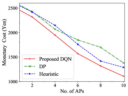
Figure 5: Monetary cost (yen) vs. No. of APs.

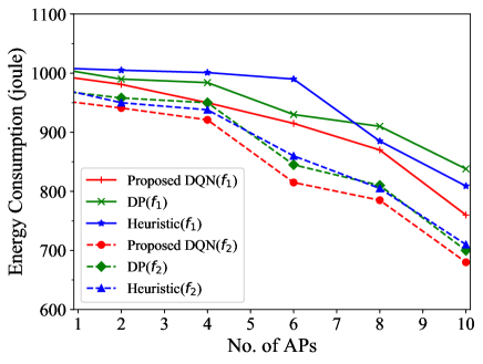
Figure 6: Energy consumption (joule) vs. No. of APs with different energy-throughput functions $f_{1}$ and $f_{2}$.

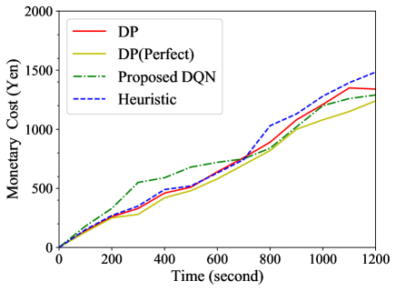
Figure 7: Monetary cost (yen) vs. Epochs.

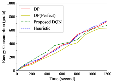
Figure 8: Energy consumption (joule) vs. Epoch with $f_{1}$.

Fig.5 shows the comparison of monetary cost among Proposed DQN, Heuristic and DP algorithms with different number of APs. Please note that we fixed the number of flows to the first three in Table 4. It can be seen that the monetary cost of Proposed DQN algorithm is lowest. The reason is also that both both Heuristic and DP algorithms can not find the optimal policy with incorrect transition probability. With a large number of wireless LAN APs deployed, the chance of using cheap wireless LAN increases. Then, the MU can reduce his monetary cost by using cheap wireless LAN. Therefore, all three algorithms’ monetary costs decreases with the number of APs.

Fig.6 shows how the MU’s energy consumption changes with the number of deployed APs under the two energy-throughput functions $f_{1}(x)$ and $f_{2}(x)$. Similar to Fig.4, the performance of Proposed DQN algorithm is the best with either $f_{1}(x)$ or $f_{2}(x)$. It shows that the energy consumptions of all three algorithms just slightly decrease with the number of APs. The reason is that the energy consumption depends on the throughput. The larger the throughput, the lower is the energy consumption. With large number of wireless LAN APs, the MU has more chance to use wireless LAN with high throughput since the average throughput of a wireless LAN is assumed as higher than that of cellular network (see Table IV).
Fig.7 and Fig.8 shows how monetary cost and energy consumption changes with time among Proposed DQN, Heuristic and DP algorithms with different number of APs. It is obvious that it takes time for the Proposed DQN to learn. The performance is not so good as Heuristic and DP. But the performance of Proposed DQN become better and better with time goes by. We also have show the performance with perfect MDP transition probability of DP algorithm, it shows that the performance of DP is best.

6 Conclusion

In this paper, we studied the multi-flow mobile data offloading problem in which a MU has multiple applications that want to download data simultaneously with different deadlines. We proposed a DQN based offloading algorithm to solve the wireless LAN offloading problem to minimize the MU’s monetary and energy cost. The proposed algorithm is effective even if the MU’s mobility pattern is unknown. The simulation results have validated our proposed offloading algorithm.

This work assumes that the MNO adopts usage-based pricing, in which the MU paid for the MNO in proportion to data usage. In the future, we will evaluate other usage-based pricing variants like tiered data plan, in which the payment of the MU is a step function of data usage. And we will also use time-dependent pricing (TDP) we proposed in [3][27], without changing the framework and algorithms proposed in this paper.

References

- [1] Cisco Systems, “Cisco visual networking index: Global mobile data traffic forecast update, 2014-2019,” Feb. 2015.
- [2] Q. C. Li, H. Niu, A. T. Papathanassiou, and G. Wu, “5G network capacity: Key elements and technologies,” IEEE Veh. Technol. Mag., vol. 9, no. 1, pp. 71–78, March 2014.
- [3] C. Zhang, B. Gu, K. Yamori, S. Xu, and Y. Tanaka, “Duopoly competition in time-dependent pricing for improving revenue of network service providers,” IEICE Trans. Commun., vol. E96-B, no. 12, pp. 2964–2975, Dec. 2013.
- [4] ——, “Oligopoly competition in time-dependent pricing for improving revenue of network service providers with complete and incomplete information,” IEICE Trans. Commun., vol. E98-B, no. 1, pp. 30–32, Jan. 2015.
- [5] J. Márquez-Barja, C. T. Calafate, J.-C. Cano, and P. Manzoni, “Review: An overview of vertical handover techniques: Algorithms, protocols and tools,” Comput. Commun., vol. 34, no. 8, pp. 985–997, June 2011.
- [6] Cisco Systems, “The future of hotspots: Making Wi-Fi as secure and easy to use as cellular,” White Paper, 2011.
- [7] Alcatel and British Telecommunications, “Wi-Fi roaming – building on andsf and hotspot2.0,” White Paper, 2012.
- [8] L. Gao, G. Iosifidis, J. Huang, L. Tassiulas, and D. Li, “Bargaining-based mobile data offloading,” IEEE J. Sel. Areas Commun., vol. 32, no. 6, pp. 1114–1125, June 2014.
- [9] G. Iosifidis, L. Gao, J. Huang, and L. Tassiulas, “A double-auction mechanism for mobile data-offloading markets,” IEEE/ACM Trans. Netw., vol. 22, no. 4, pp. 1271–1284, Aug. 2014.
- [10] A. Balasubramanian, R. Mahajan, and A. Venkataramani, “Augmenting mobile 3g using Wi-Fi,” in Proc. 8th international conference on Mobile systems, applications, and services (MobiSys 2010), June 2010, pp. 209–222.
- [11] K. Lee, J. Lee, Y. Yi, I. Rhee, and S. Chong, “Mobile data offloading: How much can Wi-Fi deliver?” IEEE/ACM Trans. Netw., vol. 21, no. 2, pp. 536–550, April 2013.
- [12] Y. Im, C. Joe-Wong, S. Ha, S. Sen, T. . Kwon, and M. Chiang, “AMUSE: Empowering users for cost-aware offloading with throughput-delay tradeoffs,” in Proc. IEEE Conference on Computer Communications (INFOCOM 2013), April 2013, pp. 435–439.
- [13] M. H. Cheung and J. Huang, “DAWN: Delay-aware Wi-Fi offloading and network selection,” IEEE J. Sel. Areas Commun., vol. 33, no. 6, pp. 1214 – 1223, June 2015.
- [14] C. Zhang, B. Gu, Z. Liu, K. Yamori, and Y. Tanaka, “A reinforcement learning approach for cost- and energy-aware mobile data offloading,” Proc. 16th Asia-Pacific Network Operations and Management Symposium (APNOMS 2016), Kanazawa, Japan, pp. 1–6, Oct. 2016.
- [15] ——, “Cost- and energy-aware multi-flow mobile data offloading using markov decision process,” IEICE Trans. Commun., vol. E101-B, no. 3, March 2018.
- [16] Z. Liu, C. Zhang, M. Dong, B. Gu, Y. Ji, and Y. Tanaka, “Markov-decision-process-assisted consumer scheduling in a networked smart grid,” IEEE Access, vol. 5, pp. 2448–2458, March 2017.
- [17] Z. Liu, G. Cheung, and Y. Ji, “Distributed markov decision process in cooperative peer-to-peer repair for WWAN video broadcast,” Proc. 2011 IEEE International Conference on Multimedia and Expo (ICME 2011), Barcelona, Spain, pp. 1–6, July 2011.
- [18] ——, “Optimizing distributed source coding for interactive multiview video streaming over lossy networks,” IEEE Trans. Circuits and Systems for Video Technology, vol. 23, no. 10, pp. 1781–1794, Oct. 2013.
- [19] P. S. Sutton and A. G. Barto, Reinforcement Learning: An Introduction, MIT Press, 1998.
- [20] V. Mnih, K. Kavukcuoglu, D. Silver, A. A. Rusu, J. Veness, M. G. Bellemare, A. Graves, M. Riedmiller, A. K. Fidjeland, G. Ostrovski, S. Petersen, C. Beattie, A. Sadik, I. Antonoglou, H. King, D. Kumaran, D. Wierstra, S. Legg, and D. Hassabis, “Human-level control through deep reinforcement learning,” Nature, vol. 518, no. 7540, pp. 529–533, Feb. 2015.
- [21] Y. LeCun, Y. Bengio, and G. Hinton, “Deep learning,” Nature, vol. 521, no. 7553, pp. 436–444, May 2015.
- [22] A. Murabito, “A comparison of efficiency, throughput, and energy requirements of wireless access points,” Report of InterOperability Laboratory, University of New Hampshire, March 2009. [Online]. Available: http://www.cisco.com/c/en/us/solutions/collateral/service-provider/visual-networking-index-vni/white{\_}paper{\_}c11-520862.pdf
- [23] S. Sen, C. Joe-Wong, S. Ha, J. Bawa, and M. Chiang, “When the price is right: enabling time-dependent pricing of broadband data,” in Proc. the 13th SIGCHI Conference on Human Factors in Computing Systems, Paris, France, May 2013, pp. 2477–2486.
- [24] A. Y. Ding, B. Han, Y. Xiao, P. Hui, A. Srinivasank, M. Kojo, and S. Tarkoma, “Enabling energy-aware collaborative mobile data offloading for smartphones,” in Proc. 10th Annual IEEE Communications Society Conference on Sensor, Mesh and Ad Hoc Communications and Networks (SECON 2013), June 2013, pp. 487–495.
- [25] N. Balasubramanian, A. Balasubramanian, and A. Venkataramani, “Energy consumption in mobile phones: a measurement study and implications for network applications,” Proc. 9th ACM SIGCOMM Conference on Internet Measurement (IMC 2009), Chicago, Illinois, USA, pp. 280–293, July 2009.
- [26] R. Bellman, Dynamic Programming, Princeton University Press, 1957.
- [27] C. Zhang, B. Gu, K. Yamori, S. Xu, and Y. Tanaka, “Oligopoly competition in time-dependent pricing for improving revenue of network service providers with complete and incomplete information,” IEICE Trans. Commun., vol. E98-B, no. 1, pp. 30–32, Jan. 2015.