The contribution of faint AGNs to the ionizing background at $z\sim 4$

Abstract

Context. Finding the sources responsible for the hydrogen reionization is one of the most pressing issues in observational cosmology. Bright QSOs are known to ionize their surrounding neighborhood, but they are too few to ensure the required HI ionizing background. A significant contribution by faint AGNs, however, could solve the problem, as recently advocated on the basis of a relatively large space density of faint active nuclei at $z>4$.

Aims. This work is part of a long term project aimed at measuring the Lyman Continuum escape fraction for a large sample of AGNs at $z\sim 4$ down to an absolute magnitude of $M_{1450}\sim-23$. We have carried out an exploratory spectroscopic program to measure the HI ionizing emission of 16 faint AGNs spanning a broad $U-I$ color interval, with $I\sim 21-23$ and $3.6<z<4.2$. These AGNs are three magnitudes fainter than the typical SDSS QSOs ($M_{1450}\lesssim-26$) which are known to ionize their surrounding IGM at $z\gtrsim 4$.

Methods. We acquired deep spectra of these faint AGNs with spectrographs available at the VLT, LBT, and Magellan telescopes, i.e. FORS2, MODS1-2, and LDSS3, respectively. The emission in the Lyman Continuum region, i.e. close to 900 Å rest frame, has been detected with S/N ratio of $\sim 10-120$ for all the 16 AGNs. The flux ratio between the 900 Å rest frame region and 930 Å provides a robust estimate of the escape fraction of HI ionizing photons.

Results. We have found that the Lyman Continuum escape fraction is between 44 and 100% for all the observed faint AGNs, with a mean value of 74% at $3.6<z<4.2$ and $-25.1\lesssim M_{1450}\lesssim-23.3$, in agreement with the value found in the literature for much brighter QSOs ($M_{1450}\lesssim-26$) at the same redshifts. The Lyman Continuum escape fraction of our faint AGNs does not show any dependence on the absolute luminosities or on the observed $U-I$ colors of the objects. Assuming that the Lyman Continuum escape fraction remains close to $\sim 75\%$ down to $M_{1450}\sim-18$, we find that the AGN population can provide between 16 and 73% (depending on the adopted luminosity function) of the whole ionizing UV background at $z\sim 4$, measured through the Lyman forest. This contribution increases to 25-100% if other determinations of the ionizing UV background are adopted from the recent literature.

Conclusions. Extrapolating these results to $z\sim 5-7$, there are possible indications that bright QSOs and faint AGNs can provide a significant contribution to the Reionization of the Universe, if their space density is high at $M_{1450}\sim-23$.

1 Introduction

One of the most pressing questions in observational cosmology is related to the reionization of neutral hydrogen (HI) in the Universe. This fundamental event marks the end of the so-called Dark Ages and is located in the redshift interval $z=6.0-8.5$. The lower limit is derived from observations of the Gunn-Peterson effect in luminous $z>6$ QSO spectra (Fan et al. 2006), while the most recent upper limit, $z<8.5$, comes from measurements of the Thomson optical depth $\tau_{e}=0.055\pm 0.009$ in the CMB polarization map by Planck (Planck Collaboration 2016). While we now have a precise timing of the reionization process, we are still looking for the sources providing the bulk of the HI ionizing photons. Obvious candidates include high-redshift star-forming galaxies (SFGs) and/or Active Galactic Nuclei (AGNs).

High-z SFGs have been advocated as the most natural way of explaining the reionization of the Universe (Robertson et al. 2015; Finkelstein et al. 2015; Schmidt et al. 2016; Parsa et al. 2018). The two critical ingredients in modeling reionization are the relative escape fraction of HI ionizing photons $f_{esc,rel}$ (and its luminosity and redshift dependence) and the number density of faint galaxies which can be measured by a precise evaluation of the faint-end slope of the UV luminosity function at high-z. Finkelstein et al. (2012, 2015) and Bouwens et al. (2016) show that an $f_{esc,rel}$ of $\geq 10-20\%$ must be assumed for all the galaxies down to $M_{1500}=-13$ in order to keep the Universe ionized at $3\leq z\leq 7$, and that the luminosity function should be steeper than $\alpha\sim-2$ in order to have a large number of faint sources. This latter assumption has been recently confirmed by the steep luminosity function found by Livermore et al. (2017) and Ishigaki et al. (2017) in the HST Frontier Fields, down to $M_{1500}=-12.5$ at $z=6$ and in the MUSE Hubble Ultra Deep Field by Drake et al. (2017), but see Bouwens et al. (2017) and Kawamata et al. (2017) for different results.

The search for HI ionizing photons escaping from SFGs has not been very successful. At $z<2$ all surveys appear to favour low $f_{esc,rel}$ from relatively bright galaxies, and recent limits on $f_{esc,rel}$ are below 1% (Grimes et al. 2009; Cowie et al. 2009; Bridge et al. 2010). At fainter magnitudes, Rutkowski et al. (2016) found that $f_{esc,rel}<5.6\%$ for $M_{1500}<-15$ ($L>0.01L^{*}$) galaxies at $z\sim 1$, concluding that these SFGs contribute less than 50% of the ionizing background. Few exceptions have been found at $z<0.4$, e.g. Izotov et al. (2016a,b) found five galaxies with $f_{esc,rel}=9-34\%$, while Leitherer et al. (2016) found two galaxies with $f_{esc,rel}=20.8-21.6\%$.

At higher redshift ($z>2$), there are contrasting results: Mostardi et al. (2013) found $f_{esc,rel}$ of $\sim 5-8$% for Lyman Break galaxies ($f_{esc,rel}\sim 18-49\%$ for Lyman-$\alpha$ emittes), but their samples could be partly contaminated by foreground objects due to the lack of high spatial resolution imaging from HST (Vanzella et al. 2010; Siana et al. 2015). Recently, three Lyman Continuum (LyC) emitters have been confirmed within the SFG population at $z\sim 3$ (Vanzella et al. 2016; Shapley et al. 2016; Bian et al. 2017). Other teams, using both spectroscopy and very deep broad or narrow band imaging from ground based telescopes and HST, give only upper limits in the range $<2-15$% (Grazian et al. 2016, 2017; Guaita et al. 2016; Vasei et al. 2016; Marchi et al. 2017; Japelj et al. 2017; Rutkowski et al. 2017). These limits cast serious doubts on any redshift evolution of $f_{esc}$, if the observed trend at $z\lesssim 3$ is extrapolated at higher-z. The low $f_{esc}$ suggests that we may have a problem in keeping the Universe ionized with just SFGs (Fontanot et al. 2012; Grazian et al. 2017; Madau 2017).

There is therefore room for a significant contribution made by AGNs at $z>3$. It is well known (see e.g. Prochaska et al. 2009; Worseck et al. 2014, Cristiani et al. 2016) that bright QSOs ($M_{1450}\leq-26$ at $z\geq 3$) are efficient producers of HI ionizing photons, and they can ionize large bubbles of HI even at distances up to several Mpc out to $z\sim 6$. However, their space density is too low at high-z to provide the cosmic photo-ionization rate required to keep the IGM ionized at $z>3$ (Fan et al. 2006; Cowie et al. 2009; Haardt & Madau 2012). The bulk of ionizing photons could then come from a population of fainter AGNs. Interestingly, the recent observations of an early and extended period for the HeII reionization at $z\sim 3-5$ by Worseck et al. (2016) seem to indicate that hard ionizing photons from AGNs, producing strongly fluctuating background on large scales, may in fact be required to explain the observed chronology of HeII reionization. Moreover, the observations of a constant ionizing UV background (UVB) from z=2 to z=5 (Becker & Bolton 2013) and the presence of long and dark absorption troughs at $z\geq 5.5$ along the lines of sight of bright $z=6$ QSOs (Becker et al. 2015) are difficult to be reconciled with a population of ionizing sources with very high space densities and low clustering, such as ultra-faint galaxies (Madau & Haardt 2015; Chardin et al. 2016, 2017). This leaves open the possibility that faint AGNs ($L\lesssim L^{*}$) at $z\geq 3-5$ could be the major contributors to the ionizing UV background.

Deep optical surveys at $z=3-5$ with complete spectroscopic information (Glikman et al. 2011) are showing the presence of a considerable number of faint AGNs ($L\lesssim L^{*}$) producing a rather steep luminosity function. This result has been confirmed and extended to fainter luminosities ($L\lesssim 0.1L^{*}$) by Giallongo et al. (2015) by means of NIR (UV rest-frame) selection of $z>4$ AGN candidates with very weak X-ray detection in the deep CANDELS/GOODS-South field (but see Parsa et al. 2018, Hassan et al. 2018, and Onoue et al. 2017 for different results). The presence of a faint ionizing population of AGNs could, if confirmed, strongly contribute to the ionizing UV background (Madau & Haardt 2015; Khaire et al. 2016), provided that a significant fraction of the produced LyC photons is free to escape from the AGN host galaxy even at faint luminosities.

Recently, the LyC $f_{esc}$ of a bright $R\leq 20.15$ AGN sample ($L\gtrsim 15L^{*}$, or $M_{1450}\leq-26$) was estimated by Cristiani et al. (2016). Approximately 80% of the sample shows large LyC emission ($f_{esc}\sim 100\%$), while $\sim$20% are not emitting at $\lambda<900$ Å rest-frame, possibly due to the presence of a broad absorption line (BAL) or associated absorption systems (e.g., Damped Lyman-$\alpha$ systems, DLAs). No trend of $f_{esc}$ with UV luminosity is detected by Cristiani et al. (2016), though the explored range in absolute magnitude is small, and there is not enough leverage to draw firm conclusions at the moment. Micheva et al. (2017) have studied the escape fraction of a small sample of $R\sim 21-26$ AGN (both type 1 and type 2) at $z\sim 3.1-3.8$ in the SSA22 region through narrow band imaging. They concluded that the contribution of these faint AGNs ($-24\lesssim M_{1450}\lesssim-22$) is not exceeding $\sim 20\%$ of the total ionizing budget. However, due to the limited depth of their narrow band UV images, the broad luminosity range and the broad redshift interval of their sample, their constraints on $f_{esc}$ for the faint AGN population are probably not conclusive. As an example, it is worth mentioning the results of Guaita et al. (2016) on faint AGNs in the CDFS region, where a large escape fraction ($\geq 46\%$) was found for 2 intermediate luminosity ($M_{1450}\sim-22$) AGNs at $z\sim 3.3$ with deep narrow band imaging, while less rigid upper limits have been measured for 6 AGNs at similar redshifts and luminosities (mean $f_{esc}\leq 45\%$).

In this paper we carry out a systematic survey of the Lyman continuum escape fraction for faint AGNs ($L\sim L^{*}$) at $3.6\leq z\leq 4.2$ through deep optical/UV spectroscopy. This redshift interval is a good compromise between minimizing the IGM absorption intervening along the line of sight and allowing observations from the ground.

This paper is organized as follows. In Sect. 2 we present the data-set, in Sect. 3 we describe the method adopted, in Sect. 4 we show the results for individual objects and for the overall sample as a whole, providing an estimate of the ionizing background produced by AGNs at $z\sim 4$. In Sect. 5 we discuss the robustness of our results and in Sect. 6 we provide a summary and the conclusions. Throughout the paper we adopt the $\Lambda$-CDM concordance cosmological model ($H_{0}=70\leavevmode\nobreak\ km/s/Mpc$, $\Omega_{M}=0.3$ and $\Omega_{\Lambda}=0.7$), consistent with recent CMB measurements (Planck collaboration 2016). All magnitudes are in the AB system.

2 Data

2.1 The AGN sample

In order to quantify the HI ionizing emission of the whole AGN population, we carried on an exploratory spectroscopic program to measure the LyC escape fraction of a small sample of faint galactic nuclei, with $I\sim 21-23$ and $3.6<z<4.2$. These AGNs are three magnitudes fainter than the typical SDSS QSOs ($M_{1450}\sim-26$) which are known to ionize their surrounding IGM at $z>3$ (Prochaska et al. 2009; Cristiani et al. 2016). At present it is not known in fact whether the escape fraction of AGN scales with their luminosity and it is not obvious that faint AGNs have the same escape fraction ($f_{esc}\sim 75-100\%$) typical of brighter QSOs.

We selected the redshift interval $3.6\leq z\leq 4.2$ for the following reasons: first, at these redshifts the mean IGM transmission is still high ($\sim 30\%$) compared to the large opacities found at $z\geq 6$ (e.g. Fan et al. 2006), which prevent a direct measurement of ionizing photons at the reionization epoch; second, at these redshifts there are a number of relatively faint AGNs ($L\lesssim L^{*}$) with known spectroscopic redshifts already available, while it is very difficult to assemble a similar sample at $z\geq 5$; third, at $z\sim 4$ sub-$L^{*}$ AGNs are still bright enough to be studied in detail with 8-10m class telescopes equipped with efficient instruments in the near UV.

Our targets have been selected from the COSMOS (Marchesi et al. 2016; Civano et al. 2016), NDWFS, DLS (Glikman et al. 2011), and the SDSS3-BOSS (Dawson et al. 2013) surveys. From the parent sample of 951 AGNs with $3.6<z_{spec}<4.2$ and $21<I<23$, we have randomly identified 16 objects with $2.0\lesssim U-I\lesssim 5.0$. These limits are approximately the minimum and maximum colors of the parent AGN sample, indicating that this small group of 16 objects is not affected by significant biases in their $f_{esc}$ properties, but represents an almost uniform coverage of the color-magnitude distribution for $z\sim 4$ AGNs. At the redshifts probed by our sample, the U filter partially covers the ionizing portion of the spectra. However, it is worth stressing that, due to the stochasticity of the IGM absorption and the broad filters adopted, it is not possible to directly translate the $U-I$ color into a robust value of $f_{esc}$, and UV spectroscopy is thus required. More precisely, the $U-I$ color distribution is a proxy for intervening absorptions rather than an indicator of LyC escape fraction for $z\sim 4$ AGNs. As we will show in the following sections, their $U-I$ colors, their apparent I-band magnitudes and their intrinsic luminosities are not biased against or in favour of objects with peculiar properties and can thus be representative of the whole population of faint AGNs at high-z. The selected AGNs cover a large interval in right ascension in order to facilitate the scheduling of the observations and are selected both in the northern and in the southern hemispheres in order to be targeted by many observational facilities, e. g. with LBT, VLT, and Magellan. The limited number (16) of selected AGNs was chosen to keep the total observing time of the order of a normal observing program (1-2 nights). This initial group of 16 AGNs with $M_{1450}<-23$ does not represent a complete sample of all the type 1 and 2 active galactic nuclei brighter than $L^{*}$, since the goal of these initial observations was first to show that the program was feasible and the requested exposure time was sufficient to estimate the LyC escape fractions of these objects with small uncertainties.

In addition to the 16 known AGN described above, we have found a serendipitous faint AGN at $z\sim 4.1$ (UDS10275) during a spectroscopic pilot project with the Magellan-II Clay telescope. Since this object is relatively bright ($I=22.27$) and the available observations cover the wavelength region where LyC is expected, we decided to include this AGN in our final sample. Unfortunately, a target observed by VLT FORS2 turned out to have a wrong spectroscopic redshift and we do not considered it in our analysis. For this reason the final sample contains 16 objects. The AGNs studied in this paper are summarised in Table 1. It is worth noting here that we systematically avoid observing QSOs classified as Broad Absorption Line from published spectroscopy, since we expect no LyC photons escaping from them. As discussed later in Sect. 5, this choice is not biasing the results reached in the present work.

Fig.1 shows the $U-I$ color versus the observed I-band magnitude for the AGNs at $3.6<z<4.2$ studied in this paper. Table 1 summarises the properties of these faint AGNs.

Figure 1: The $U-I$ color vs the observed I-band magnitude for the AGNs studied in this work. Squares show the targets observed with FORS2 at the VLT telescope, triangles are the AGNs observed with MODS1-2 at the LBT telescope, while pentagons are the AGNs observed with the LDSS3 instrument at the Magellan-II Clay telescope. Three objects from Table 1 have no information on the U-band magnitude and are not plotted here. We do not plot COSMOS1710 since it is not at redshift $\sim 4$.

Table 1: The AGN sample

Name	$z_{spec}^{orig}$	magI	magU	$Log(L_{X})$	Telescope	RA	DEC	$t_{exp}$
		(AB)	(AB)	2-10 keV		J2000	J2000	hour
SDSS36	4.047	21.01	24.26	n.a.	LBT	01:47:57.46	+27:33:26.8	2.5
SDSS32	3.964	20.88	23.56	n.a.	LBT	13:29:26.58	+28:14:12.9	1.75
COSMOS775	3.609	21.71	24.63	44.38	LBT	09:57:53.49	+02:47:36.2	3.5
SDSS37	4.173	21.16	23.37	n.a.	LBT	15:32:36.78	+27:51:54.8	3.5
NDWFSJ05	3.900	21.95	-99.0${}^{a}$	n.a.	LBT	14:36:42.86	+35:09:23.8	5.5
SDSS04	3.772	21.31	23.21	n.a.	VLT	09:32:29.6	-01:32:32.6	1.5
COSMOS1782	3.748	22.65	25.94	44.26	VLT	10:02:48.9	+02:22:12.0	1.5
SDSS20	3.899	21.26	23.89	n.a.	VLT	12:12:48.3	-01:01:56.3	0.83
SDSS27	3.604	21.63	24.41	n.a.	VLT	12:49:42.7	-01:37:22.5	0.25
COSMOS955	3.715	21.25	26.14	44.71	VLT	10:00:50.2	+02:26:18.5	2.17
COSMOS1311	3.717	21.38	-99.0${}^{a}$	44.37	VLT	10:01:02.3	+02:22:34.1	2.17
COSMOS1710	3.567${}^{b}$	22.78	23.98	n.a.	VLT	10:02:52.1	+01:55:48.5	1.7
SDSS3777	3.723	21.28	25.49	n.a.	Magellan	12:16:44.6	-01:06:54.4	1.5
SDSS3793	3.743	21.40	25.33	n.a.	Magellan	12:43:59.8	-01:59:53.4	2.3
SDSS3785	3.769	21.29	25.42	n.a.	Magellan	10:30:19.0	-02:54:56.6	1.3
SDSS3832	3.663	21.15	25.83	n.a.	Magellan	10:26:31.6	-00:55:29.7	1.3
UDS10275	4.096	22.27	-99.0${}^{a}$	n.a.	Magellan	02:18:05.7	-05:26:35.8	1.7

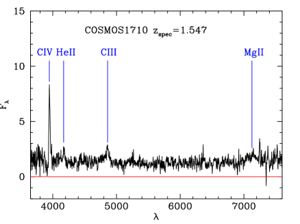
Figure 8: The UV spectrum of AGN COSMOS1710 by VLT FORS2. The spectroscopic redshift for this source in Marchesi et al. (2016) and Civano et al. (2016) turns out to be wrong. The correct redshift is $z_{spec}=1.547$, thanks to many high-ionization lines detected in the spectrum (CIV, HeII, CIII, MgII, marked by the blue vertical lines).

The spectroscopic redshifts $z_{spec}^{orig}$ have been taken from Dawson et al. (2013), Glikman et al. (2011), Marchesi et al. (2016), and Civano et al. (2016). The spectroscopic redshift for UDS10275 has been derived by the Magellan data described in this paper. The X-ray luminosity for the AGNs in the COSMOS field has been taken from Civano et al. (2016). Notes on individual objects: (a) The U band magnitude for this object is not available. (b) COSMOS1710 had a spectroscopic redshift $z_{orig}=3.567$ from the work by Marchesi et al. (2016) and Civano et al. (2016), but from our deep FORS2 spectrum we derive an updated spectroscopic redshift of $z=1.547$ (see Fig.8). This object is not included in our final sample where we have measured the LyC escape fraction for AGN at $z\gtrsim 3.6$.

2.2 Observations

We observed 5 objects with 22 hours of exposure in service mode with the MODS1-2 optical spectrographs at the LBT telescope and 7 targets with FORS2 (with the blue enhanced CCDs) at the ESO VLT telescope, in 2 nights in visitor mode (Program 098.A-0862, PI A. Grazian). During several nights at the Magellan-II Clay telescope we observed 4 targets with the LDSS3 spectrograph, and we discovered one faint AGN at $z\sim 4$ during a pilot project. In total, we collected a sample of 16 relatively faint AGNs at $3.6<z<4.2$, which is summarised in Table 1. The adopted exposure time per target varies according to the I band magnitudes and to the U-I colors of the AGNs.

2.2.1 LBT MODS

During the observing period LBT2016 (Program 30; PI A. Grazian), we carried out deep UV spectroscopy of 5 faint AGNs (Fig.1, triangles) down to an absolute magnitude $M_{1450}=-24.0$ ($L\sim 2L^{*}$) at $3.6<z<4.2$ with the LBT double spectrographs MODS1-2 (Pogge et al. 2012; Rothberg et al. 2016).

MODS is a unique instrument, since it is very efficient in the $\lambda_{obs}\sim 4000$ Å region, and it allows to observe in a single exposure the whole optical spectrum, from $\lambda\sim 3400$ Å to $\sim 10000$ Å, which is essential for the goal of this paper. We have used MODS1-2, with the Blue (G400L) and Red (G670L) Low-Resolution gratings fed by the dichroic, reaching a resolution of $R\sim 1000$ for the adopted slit of 1.2 arcsec. The dispersion of the spectra is 0.5 Å/px for the G400L grating in the blue beam, and 0.8 Å/px for the G670L grating in the red beam, respectively.

The blue side of the MODS1-2 spectra was used to quantify the LyC escape fraction, sampling the spectral region blue-ward of 912 Å rest-frame, while the red part ($\lambda\sim 6000-10000$ Å) was used to fit the continuum at $\lambda_{rest}\sim 1500-2000$ Å of each AGN with a power law. The simultaneous observations of the blue and red spectra also allowed to get rid of variability effects which are affecting the escape fraction studies based on photometry taken in different epochs (e.g. Micheva et al. 2017). The simultaneous availability of the blue and the red spectra also allowed us to increase the survey speed by a factor of 2, with respect to traditional optical spectrographs on 8m class telescopes (i.e. FORS2 at VLT). Moreover, since the observations were executed in the “Homogeneous Binocular” mode (i.e. with MODS1 and MODS2 pointing on the same position on the sky with the same configuration), by observing the same target with the two spectrographs the survey speed gained another factor of 2, for a total net on-target time of 17 hours for 5 faint AGNs.

The LBT observations were executed in service mode by a dedicated team under the organization of the LBT INAF Coordination center. The average seeing during observations was around 1.0 arcsec, with airmass less than 1.3 and dark moon ($\leq 7$ days) in order to go deep in the UV side of the spectra.

The MODS1-2 spectrographs have been used in long slit spectroscopic mode, since our targets are sparse in the sky and do not fall on the same field of view. A dithering of $\pm 1.5$ arcsec along the slit length was carried out in order to improve the sky subtraction and flat-fielding. The dithered observations were repeated several times, splitting each observation in sequence of 900 sec exposures.

The relative flux calibration was obtained by observing the spectro-photometric standard Feige34 for each observing night. The standard calibration frames (bias, flat, lamps for wavelength calibration) have been obtained during day-time operation.

2.2.2 VLT FORS2

During the observing period ESO P98 (Program 098.A-0862; PI A. Grazian), we obtained deep FORS2 spectroscopy in visitor mode for 7 faint AGNs (Fig.1, squares) down to an absolute magnitude $M_{1450}=-23.3$ ($L\sim L^{*}$). Two nights of VLT (21-22 of February, 2017) were assigned to our program. We used FORS2 with the blue optimized CCD in visitor mode. Among the VLT instruments, the blue optimized FORS2 is the only UV sensitive instrument that can be used for such scientific application. We adopted a slit width of 1.0 arcsec with the grism 300V (without the sorting order filter) which, coupled with the E2V blue optimized CCD, guarantees the maximum efficiency in the UV spectral region.

The typical seeing during observations was 0.6-1.4 arcsec, with partial thin clouds for the majority of the observing run. The adopted configuration allows us to cover the spectral window from 3400 to 8700 Å, centered at 5900 Å, with a dispersion of 3.4 Å/px and a resolution of $R\sim 400$. Exposure times ranged from 15 minutes to 2.2 hours, depending on the faintness of the targets and on their $U-I$ color. Each observation was split in exposures of 1350 seconds, following an ABBA dithering pattern of $\pm 1.5$ arcsec, in order to properly subtract the sky background and to carry out an accurate flat-fielding of the data.

At the beginning of the first night, the spectro-photometric standard star Hilt600 was observed in order to obtain a relative flux calibration of the targeted AGNs. All the remaining calibration frames (bias, flat, lamps for wavelength calibration) were obtained during day-time operations at the end of each observing night.

Three targets (SDSS04, SDSS20, SDSS27) were observed in long slit configuration, while the remaining AGNs (COSMOS955, COSMOS1311, COSMOS1710, COSMOS1782) were observed with multi object spectroscopy (MXU): in the COSMOS pointings, indeed, there are also many X-ray sources from Marchesi et al. (2016) and Civano et al. (2016) without spectroscopic identification. Given the legacy value of these targets, we carried out MXU observations in order to measure the redshifts of these fillers.

2.2.3 Magellan LDSS3

We used the LDSS3 spectrograph, mounted at the Magellan-II Clay 6.5m telescope at Las Campanas observatory (LCO), in February and March 2017 to observe 4 SDSS AGNs with I-band magnitude in the interval $21.0\leq I\leq 21.5$. We chose the grism VPH-Blue, with peak sensitivity around 6000 Å, wavelength coverage between 3800 and 6500 Å and a resolution $R\sim 1400$ for a slit of 1 arcsec width. The typical seeing during observations was 0.6-0.9 arcsec, matching the slit width of 1.0 arcsec. Each observation was split in exposures of 900 seconds, without any dithering pattern. The observations were taken under non-optimal condition w.r.t. the lunar illumination, with a slightly high background in the UV. Moreover, the sensitivity of LDSS3 (equipped with red sensitive detectors) drops around 4000 Å rest frame, where the LyC of $z\sim 4$ sources is expected. For these reasons, we decided to observe relatively bright candidates in order to improve the number statistics by enlarging our sample.

In September 2017 a relatively faint AGN (UDS10275, $I\sim 22.3$) at $z\sim 4.1$ has been serendipitously observed with the VPH-All grism and the LDSS3 instrument mounted at the Magellan-II Clay 6.5m telescope. The sensitivity of this grism peaks at $\lambda=7000$ Å and covers the wavelength range between 4200 and 10000 Å. While the sensitivity in the blue is slightly reduced w.r.t. the VPH-Blue grism, it allows to cover a relatively larger spectral window, which is useful for the characterization of the properties of this target. With an exposure time of approximately 2 hours we were able to detect flux in the LyC region, as we will discuss in detail in the following sections.

3 The Method

3.1 Data Reduction

The AGN spectra obtained with MODS1-2 were reduced by the INAF LBT Spectroscopic Reduction Center based in Milano.

The LBT spectroscopic pipeline was developed inheriting the functionalities from the VIMOS pipeline (Scodeggio et al. 2005; Garilli et al. 2012), and was modified for the specific case of the dual MODS instruments. The pipeline corrects the science frames with basic pre-reduction (bias, flat field, wavelength calibration in two dimensions) and subtracts the sky from each frame by fitting the background with a polynomial function in 2D, which takes into account the slit distortions. The relative flux calibration was carried out by computing the spectral response function thanks to the observations of the spectro-photometric standard star Feige34. Fully calibrated 2D and 1D extracted spectra with their associated RMS maps were produced at the end for each target, stacking all the available LBT observations after the cosmic ray rejection.

The FORS2 data were reduced with a custom software, developed on the basis of the MIDAS package (Warmels 1991). These tools are similar to the one described in Vanzella et al. (2008). Briefly, the frames have been pre-reduced with the bias subtraction and the flat fielding. For each slit, the sky background was estimated with a second order polynomial fitting. The sky fit was computed independently in each column within two free windows, above and below the position of the object. In the case of multiple exposures of the same source, the one dimensional spectra were co-added weighing according to the exposure time, the seeing condition and the resulting quality of each extraction process. Spatial median filtering was applied to each dithered exposures to eliminate the cosmic rays. Wavelength calibration was calculated on day-time arc calibration frames, using four arc lamps (He, HgCd, and two Ar lamps) providing sharp emission lines over the whole spectral range observed. The object spectra were then rebinned to a linear wavelength scale. Relative flux calibration was achieved by observations of the standard star Hiltner 600. For each reduced science spectrum we created also an RMS spectrum.

The data acquired with the LDSS3 instrument were reduced using the same custom package adopted to reduce the FORS2 data, deriving the relative flux calibrations through the spectro-photometric standard stars EG274 and LTT4816.

Fig.2-8, Fig.9-13, and Fig.14-18 show the AGN spectra obtained with FORS2 at VLT, MODS1-2 at LBT, and LDSS3 at Magellan telescope, respectively, as described in Table 1. In each spectrum, the blue region shows the spectral window covering LyC emission, i.e. at $\lambda\leq 912$ Å rest frame. The Magellan and LBT spectra have been smoothed by a boxcar filter of 5 pixels for aesthetic reasons only, in order to match the spectral resolution with the effective resolution of the pictures.

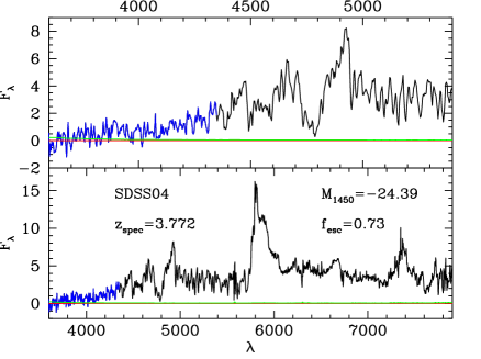
Figure 2: Bottom: The UV/optical spectrum of the AGN SDSS04 observed by FORS2 at VLT. Top: A zoom of the blue side of the spectrum for AGN SDSS04. The red horizontal lines mark the zero level for the flux $F_{\lambda}$, in arbitrary unit. The LyC region (at $\lambda\leq 912$ Å rest frame) has been highlighted in blue. The associated RMS is shown by the green spectrum.

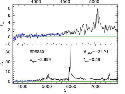
Figure 3: Bottom: The UV/optical spectrum of the AGN SDSS20 observed by FORS2 at VLT. Top: A zoom of the blue side of the spectrum for AGN SDSS20. The red horizontal lines mark the zero level for the flux $F_{\lambda}$, in arbitrary unit. The LyC region (at $\lambda\leq 912$ Å rest frame) has been highlighted in blue. The associated RMS is shown by the green spectrum.

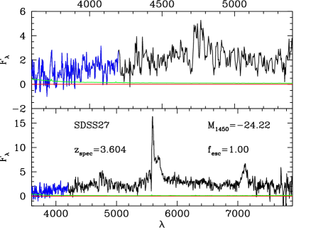
Figure 4: Bottom: The UV/optical spectrum of the AGN SDSS27 observed by FORS2 at VLT. Top: A zoom of the blue side of the spectrum for AGN SDSS27. The red horizontal lines mark the zero level for the flux $F_{\lambda}$, in arbitrary unit. The LyC region (at $\lambda\leq 912$ Å rest frame) has been highlighted in blue. The associated RMS is shown by the green spectrum.

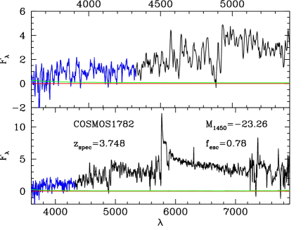
Figure 5: Bottom: The UV/optical spectrum of the AGN COSMOS1782 observed by FORS2 at VLT. Top: A zoom of the blue side of the spectrum for AGN COSMOS1782. The red horizontal lines mark the zero level for the flux $F_{\lambda}$, in arbitrary unit. The LyC region (at $\lambda\leq 912$ Å rest frame) has been highlighted in blue. The associated RMS is shown by the green spectrum.

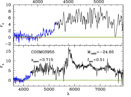
Figure 6: Bottom: The UV/optical spectrum of the AGN COSMOS955 observed by FORS2 at VLT. Top: A zoom of the blue side of the spectrum for AGN COSMOS955. The red horizontal lines mark the zero level for the flux $F_{\lambda}$, in arbitrary unit. The LyC region (at $\lambda\leq 912$ Å rest frame) has been highlighted in blue. The associated RMS is shown by the green spectrum.

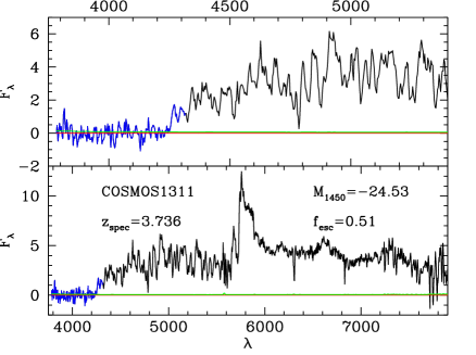
Figure 7: Bottom: The UV/optical spectrum of the AGN COSMOS1311 observed by FORS2 at VLT. Top: A zoom of the blue side of the spectrum for AGN COSMOS1311. The red horizontal lines mark the zero level for the flux $F_{\lambda}$, in arbitrary unit. The LyC region (at $\lambda\leq 912$ Å rest frame) has been highlighted in blue. The associated RMS is shown by the green spectrum.

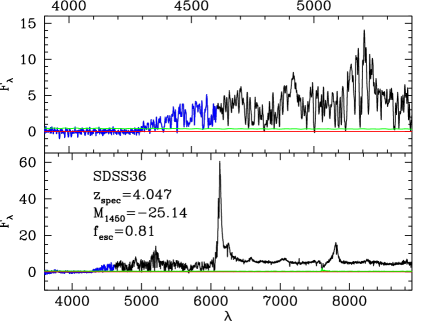
Figure 9: Bottom: The UV/optical spectrum of the AGN SDSS36 observed by MODS1-2 at LBT. Top: A zoom of the blue side of the spectrum for AGN SDSS36. The red horizontal lines mark the zero level for the flux $F_{\lambda}$, in arbitrary unit. The LyC region (at $\lambda\leq 912$ Å rest frame) has been highlighted in blue. The associated RMS is shown by the green spectrum. The scientific data have been smoothed by a boxcar filter of 5 pixels.

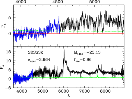
Figure 10: The UV/optical spectrum of AGN SDSS32 by LBT MODS1-2. The LyC region (at $\lambda\leq 912$ Å rest frame) has been highlighted in blue. The associated RMS is shown by the green spectrum. The scientific data have been smoothed by a boxcar filter of 5 pixels.

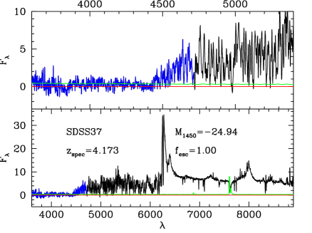
Figure 11: The UV/optical spectrum of AGN SDSS37 by LBT MODS1-2. The LyC region (at $\lambda\leq 912$ Å rest frame) has been highlighted in blue. The associated RMS is shown by the green spectrum. The scientific data have been smoothed by a boxcar filter of 5 pixels.

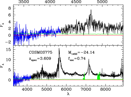
Figure 12: The UV/optical spectrum of AGN COSMOS755 by LBT MODS1-2. The LyC region (at $\lambda\leq 912$ Å rest frame) has been highlighted in blue. The associated RMS is shown by the green spectrum. The scientific data have been smoothed by a boxcar filter of 5 pixels.

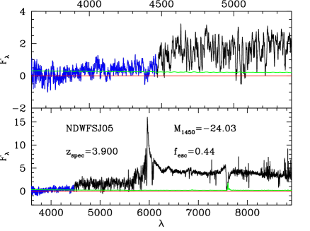
Figure 13: The UV/optical spectrum of AGN NDWFSJ05 by LBT MODS1-2. The LyC region (at $\lambda\leq 912$ Å rest frame) has been highlighted in blue. The associated RMS is shown by the green spectrum. The scientific data have been smoothed by a boxcar filter of 5 pixels.

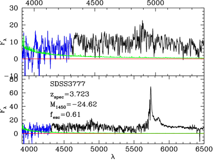
Figure 14: Bottom: The whole spectrum of the AGN SDSS3777 observed by LDSS3 at Magellan. Top: A zoom of the blue side of the spectrum for AGN SDSS3777. The red horizontal lines mark the zero level for the flux $F_{\lambda}$, in arbitrary unit. The LyC region (at $\lambda\leq 912$ Å rest frame) has been highlighted in blue. The associated RMS is shown by the green spectrum. The scientific data have been smoothed by a boxcar filter of 5 pixels.

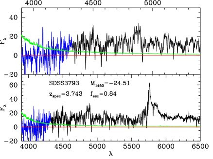
Figure 15: Bottom: The whole spectrum of the AGN SDSS3793 observed by LDSS3 at Magellan. Top: A zoom of the blue side of the spectrum for AGN SDSS3793. The red horizontal lines mark the zero level for the flux $F_{\lambda}$, in arbitrary unit. The LyC region (at $\lambda\leq 912$ Å rest frame) has been highlighted in blue. The associated RMS is shown by the green spectrum. The scientific data have been smoothed by a boxcar filter of 5 pixels.

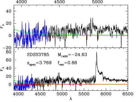
Figure 16: Bottom: The whole spectrum of the AGN SDSS3785 observed by LDSS3 at Magellan. Top: A zoom of the blue side of the spectrum for AGN SDSS3785. The red horizontal lines mark the zero level for the flux $F_{\lambda}$, in arbitrary unit. The LyC region (at $\lambda\leq 912$ Å rest frame) has been highlighted in blue. The associated RMS is shown by the green spectrum. The scientific data have been smoothed by a boxcar filter of 5 pixels.

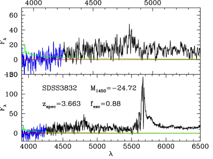
Figure 17: Bottom: The whole spectrum of the AGN SDSS3832 observed by LDSS3 at Magellan. Top: A zoom of the blue side of the spectrum for AGN SDSS3832. The red horizontal lines mark the zero level for the flux $F_{\lambda}$, in arbitrary unit. The LyC region (at $\lambda\leq 912$ Å rest frame) has been highlighted in blue. The associated RMS is shown by the green spectrum. The scientific data have been smoothed by a boxcar filter of 5 pixels.

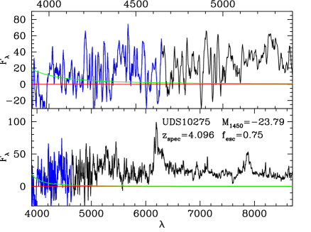
Figure 18: Bottom: The whole spectrum of the AGN UDS10275 observed by LDSS3 at Magellan. Top: A zoom of the blue side of the spectrum for AGN UDS10275. The red horizontal lines mark the zero level for the flux $F_{\lambda}$, in arbitrary unit. The LyC region (at $\lambda\leq 912$ Å rest frame) has been highlighted in blue. The associated RMS is shown by the green spectrum. The scientific data have been smoothed by a boxcar filter of 5 pixels.

3.2 Estimating the Lyman Continuum escape fraction of the faint AGNs

For each object in Table 1 the following measurements have been carried out. First, we refine the input spectroscopic redshift by measuring the position of the OI 1305 emission line, which gives the systemic redshift. When this line is weak, we keep the original redshift $z_{spec}^{orig}$ provided in Table 1, otherwise the updated redshift $z_{spec}^{new}$ can be found in Table 2. The exact determination of the systemic redshift for our AGNs is important since it allows us to measure precisely the position of the 912 Å break, and thus an accurate estimate of the LyC escape fraction for our objects. Only for the AGNs COSMOS1311 and SDSS04 the spectroscopic redshifts have been revised by small amounts, $\Delta z\sim 0.019$ and $-0.004$ respectively. The AGN COSMOS1710 instead had a wrong spectroscopic redshift in Marchesi et al. (2016) and Civano et al. (2016) and was discarded in the following analysis.

After the refinement of the spectroscopic redshifts, we compute for each AGN in our sample the LyC escape fraction. We decided to adopt the technique outlined in Sargent et al. (1989) in order to measure $f_{esc}=exp(-\tau_{LL})$ from the spectra, where $\tau_{LL}$ is the opacity of the associated Lyman limit (LL). Precisely, we estimate the mean flux above and below the Lyman limit (912 Å rest frame) and measure the escape fraction as $f_{esc}=f_{\nu}(900)/f_{\nu}(930)$, where $f_{\nu}(900)$ is the mean flux of the AGN in the Lyman continuum region, namely between 892 and 905 Å rest frame, while $f_{\nu}(930)$ is the average flux in the non ionizing region redward of the LL, between 915 and 945 Å rest frame, avoiding the region between 935 and 940 Å due to the presence of the Lyman-$\epsilon$ emission line. These average fluxes have been computed through an iterative clipping of spectral regions deviating more than 2 $\sigma$ from the mean flux values, as shown in Fig.19 for AGN SDSS36. This method allows us to avoid spectral regions affected by some intervening strong IGM absorption systems or contaminated by emission lines. Similarly to Prochaska et al. (2009), we do not use the wavelength range close to the Lyman limit (905-912 Å rest frame) since it can be affected by the AGN proximity effect. In principle, the AGN proximity zone is a signature of ionizing photons escaping into the IGM, and should be considered in these calculation. However, we do not want to work too close to 912 Å rest frame in order to avoid biases due to possible wrong estimates of the spectroscopic redshift. For this reason the LyC $f_{esc}$ provided in Table 2 should be considered as a robust lower limit for the real value.

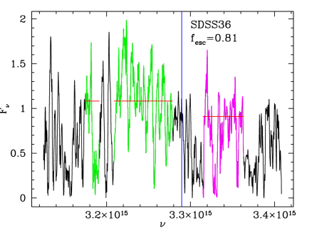
Figure 19: The estimate of the LyC escape fraction for the AGN SDSS36 observed with MODS1-2 at the LBT telescope. The spectrum is in $F_{\nu}$ and it is arbitrarily normalized and blueshifted to $z=0$ (rest frame frequencies). The green portion of the spectrum shows the spectral region between 915 and 945 Å rest frame (excluding the wavelength range 935-940 Å due to the presence of the Lyman-$\epsilon$ emission line), while the magenta portion indicates the ionizing photons emitted between 892 and 905 Å rest frame. The blue vertical line indicates the location of the 912 Å rest frame break. The red horizontal lines mark the mean values above and below the Lyman limit, after the iterative 2-$\sigma$ clipping. The resulting escape fraction is the ratio between these two mean fluxes, and turns out to be $81\%$ for SDSS36.

This technique is different compared to the method adopted by Cristiani et al. (2016). They fit the SDSS QSO spectra with a power law in the wavelength range between 1284 and 2020 Å rest frame, avoiding the region affected by strong emission lines, and then extrapolate the fitted spectrum blueward of the Lyman-$\alpha$ line. After correcting for the spectral slope, they apply a mean correction for IGM absorption adopting the recipes of Inoue et al. (2014). Finally they computed the escape fraction as the mean flux between 865 and 885 Å rest frame, after normalizing the spectra to 1.0 redward of the Lyman-$\alpha$. Since they apply an average correction for the IGM extinction, the LyC escape fraction of their bright QSOs goes from 0.0 to 2.5 (250%, see their Fig. 7). The values above 100% are simply due to the fact that in some QSOs the actual IGM absorption is lower than the mean value provided by Inoue et al. (2014). Since we do not want to rely on assumptions regarding the IGM properties surrounding our AGNs, we decided to adopt the technique of Sargent et al. (1989) outlined above, which gives a robust lower limit for the LyC escape fraction.

Finally we computed the absolute magnitude of our AGNs at 1450 Å rest frame starting from the observed I band magnitude in Table 1, $M_{1450}=I-5\log_{10}(D_{L})+5+2.5\log_{10}(1+z_{spec})$, where $D_{L}$ is the luminosity distance of the object and $z_{spec}$ is the refined spectroscopic redshift. At $z\sim 4$ the I band is sampling directly the 1450 Å rest frame, thus minimizing the K-correction effects.

Table 2 summarises the measured properties (refined spectroscopic redshift, LyC escape fraction, absolute magnitude $M_{1450}$) of the faint AGNs in our sample.

Table 2: The measured properties of faint AGNs in our sample

Name	$z_{spec}^{new}$	$f_{esc}(LyC)$	S/N	$M_{1450}$
SDSS36	4.047	0.81	87	-25.14
SDSS32	3.964	0.86	33	-25.13
COSMOS775	3.609	0.74	31	-24.14
SDSS37	4.173	1.00	121	-24.94
NDWFSJ05	3.900	0.44	12	-24.03
SDSS04	3.768	0.73	96	-24.39
COSMOS1782	3.748	0.78	72	-23.26
SDSS20	3.899	0.53	58	-24.71
SDSS27	3.604	1.00	42	-24.22
COSMOS955	3.715	0.51	84	-24.65
COSMOS1311	3.736	0.51	29	-24.53
SDSS3777	3.723	0.61	26	-24.62
SDSS3793	3.743	0.84	12	-24.51
SDSS3785	3.769	0.88	20	-24.63
SDSS3832	3.663	0.88	11	-24.72
UDS10275	4.096	0.75	27	-23.80
MEAN	3.82	0.74		-24.46

The LyC escape fraction $f_{esc}(LyC)$ and the absolute magnitude $M_{1450}$ have been derived adopting the refined spectroscopic redshift $z_{spec}^{new}$. The S/N ratio refers to the total flux in the LyC region, integrated between 892 and 905 Å rest frame. The errors on $f_{esc}(LyC)$ vary from $\sim$2 to 15%, according to the measured S/N ratio.

4 Results on the LyC escape fraction of high-z AGNs

The results summarised in Table 2 indicate that we detect a LyC escape fraction between 44% and 100% for all the 16 observed AGNs with absolute magnitude in the range $-25.14\leq M_{1450}\leq-23.26$. From a quantitative analysis of the spectra shown in Fig.2 and 9, as well as those in the Appendix, we confirm that the detection of HI ionizing flux is significant for all the observed AGNs, with a S/N ratio between 11 and 121 for our targets. The uncertainties on the measured LyC escape fraction in Table 2 are of few percents ($\sim 2-15\%$). The very good quality of these data has been allowed by the usage of efficient spectrographs in the UV wavelengths and by the long exposure time dedicated to this program (see Table 1). For the AGNs observed with the Magellan-II telescope the S/N is slightly lower, S/N$\sim 11-27$, due to the non optimal conditions during the observations (high moon illumination).

With these spectra we confirm the detection of ionizing radiation for all the 16 observed AGN, with a mean LyC escape fraction of $\sim 74\%$ and a dispersion of $\pm 18\%$ at 1$\sigma$ level. The latter should not be considered as the uncertainty on the $f_{esc}$ measurements, but the typical scatter of the observed AGN sample.

4.1 Dependence of LyC escape fraction on AGN luminosity and U-I color

Fig.20 shows the dependence of the escape fraction on the absolute magnitude $M_{1450}$ of the faint AGNs in our sample (filled triangles, squares, and pentagons). No particular trend with the absolute magnitude is observed in our data. In order to extend the baseline for the AGN luminosities, we adopt as reference the mean value of the escape fraction derived by Cristiani et al. (2016) for a sample of 1669 bright QSOs at $z\sim 4$ from the SDSS survey. They obtain a mean escape fraction of 75% for $M_{1450}\lesssim-26$, which is a luminosity $\sim$10 times larger than our faint limit $M_{1450}\leq-23.26$. As evident from Fig.20, no trend of the escape fraction of ionizing photons with the luminosity of the AGN/QSOs is detected. It is interesting to note that the quoted value for Cristiani et al. (2016) of $M_{1450}\lesssim-26$ represents the faint limit of the 1669 SDSS QSOs analysed, and their sample extends towards brighter limits $M_{1450}\sim-29$. Moreover, in Sargent et al. (1989) there are two QSOs (Q0000-263 and Q0055-264) with redshift $z>3.6$ and absolute magnitude of -29.0 and -30.2, with escape fraction close to 100%, and one QSO (Q2000-330) with $M_{1450}=-29.8$ and $f_{esc}\sim 70\%$. Finally, it is worth noting that the value of escape fraction provided in Table 2 are bona fide lower limits to the ionizing radiation, which can be even higher than 80% and possibly close to 100%, if we take into account all the possible corrections (i.e., proximity effect, absorbers close to the LLS, intrinsic spectral slopes), as we will discuss in Section 5.

Figure 20: The dependence of the LyC escape fraction on the absolute magnitude $M_{1450}$ for QSOs and AGNs at $3.6\leq z\leq 4.2$. Squares show the targets observed with the VLT telescope, triangles are the AGNs observed with MODS1-2 at the LBT telescope, while pentagons are the AGNs observed with the LDSS3 instrument at the Magellan-II Clay telescope. The uncertainties on the measured LyC escape fraction at $M_{1450}\gtrsim-25$ are of few percents ($\sim 2-15\%$). The two asterisks connected by an horizontal line show the range of $M_{1450}$ for the QSOs studied by Cristiani et al. (2016, C16), while the three stars are three very bright QSOs ($M_{1450}\sim-30$) studied by Sargent et al. (1989, S89). No obvious trend of $f_{esc}$ with the absolute magnitude $M_{1450}$ is detected.

The outcome of Fig.20 is that the LyC escape fraction of QSOs and their fainter version (AGNs) does not vary in a wide luminosity range, between $M_{1450}\sim-30$ down to $M_{1450}\sim-23$, which is a factor of $10^{3}$ in luminosity. More interestingly, we are reaching luminosities $\lesssim L^{*}$ at $z\sim 4$, which should provide the bulk of the emissivity at 1450 Å rest frame (Giallongo et al. 2012, 2015).

Figure 21: The dependence of LyC escape fraction on the observed U-I color for our faint AGNs. No obvious trend has been detected. Three objects from Table 1 have no information on the U-band magnitude and are not plotted here.

Fig.21 shows the LyC escape fraction of our faint AGNs versus the observed U-I color. No obvious trend is present, indicating that the typical color selection for $z\sim 4$ AGNs is not causing a notable effect on the LyC transmission for our sample.

The fact that we do not find any change in the properties of the escape fraction of faint AGNs ($L\sim L^{*}$) with respect to the brighter QSO sample ($L\sim 10^{3}L^{*}$) possibly indicates that even fainter AGNs ($L\sim 10^{-2}L^{*}$) at $z\sim 4$ could have an escape fraction larger than 75% and possibly close to 100%. Although a gradual decrease of the escape fraction with decreasing luminosity would be expected by AGN feedback models (see e.g. Menci et al. 2008, Giallongo et al. 2012), this trend becomes milder as the redshift increases especially at $z>4$. For this reason, in the following we assume that AGNs brighter than $L\sim 10^{-2}L^{*}$ ($M_{1450}\sim-18$) have $f_{esc}\sim 75\%$. In a similar way, Cowie et al. (2009) and Stevans et al. (2014) show values of $f_{esc}$ close to unity both for bright QSOs and for much fainter Seyfert galaxies at lower redshifts. We will use this assumption in the next sections to derive the contribution of the faint AGN population to the ionizing background at $z\sim 4$ and to make some speculations on the role of accreting SMBHs to the reionization process at higher redshifts.

4.2 The HI ionizing background at $z\sim 4$ produced by faint AGNs

In order to evaluate the contribution of faint AGNs to the HI ionizing background at $z\sim 4$ we assume that the LyC escape fraction is at least 75% for all the accreting SMBHs, from $M_{1450}=-28$ down to $M_{1450}=-18$, which correspond approximately to a luminosity range $10^{-2}L^{*}\leq L\leq 10^{2}L^{*}$, as carried out by Giallongo et al. (2015).

We use the same method adopted by Giallongo et al. (2015) to compute the UVB (in units of $10^{-12}$ photons per second, $\Gamma_{-12}$) starting from the AGN luminosity function and assuming a mean free path of 37 proper Mpc at $z=4.0$, in agreement with Worseck et al. (2014). At this aim, we adopt a spectral slope $\alpha_{\nu}$ of -0.44 between 1200 and 1450 Å rest frame and -1.57 below 1200 Å rest frame, following Schirber & Bullock (2003). As discussed in Giallongo et al. (2015) and Cristiani et al. (2016), this choice is almost equivalent to assume a shallower slope of -1.41 below 1450 Å, as found by Shull et al. (2012) and Stevans et al. (2014).

In Table 3 we compute the value of the HI ionizing UVB $\Gamma_{-12}$ assuming $f_{esc}(LyC)=75\%$ and considering different parameterizations of the $z=4$ AGN luminosity function according to the different renditions found in the recent literature (Glikman et al. 2011; Giallongo et al. 2015; Akiyama et al. 2017; Parsa et al. 2018). When these luminosity functions are centered in a different redshift bin, we shift them to z=4 applying a density evolution of a factor of 3 per unit redshift (i.e. $10^{-0.43z}$), according to the results provided by Fan et al. (2001) for the density evolution of bright QSOs. Here we assume that the bright and faint AGN populations evolve at the same rate, which may not be completely true (e.g. AGN downsizing, see Hasinger et al. 2005).

We provide the HI photo-ionization rate both at $M_{1450}\leq-23$ and at $M_{1450}\leq-18$. The values in parenthesis show the fraction of the UVB contributed by QSOs ad AGNs w.r.t. the value of $\Gamma_{-12}=0.85$ found by Becker & Bolton (2013, hereafter BB13) at z=4. This value is required to keep the Universe ionized at these redshifts. If we adopt a UVB of $\Gamma_{-12}=0.55$ found by Faucher-Giguere et al. (2008, hereafter FG08) at $z=4$, then the fractional values in Table 3 should be increased by a factor of 1.55.

Table 3: The HI photo-ionization rate $\Gamma_{-12}$ produced by AGN at $z\sim 4$

Luminosity Function	$\Gamma_{-12}$	$\Gamma_{-12}$
	$M_{1450}\leq-23$	$M_{1450}\leq-18$
Glikman et al. (2011)	0.140 (16.5%)	0.307 (36.3%)
Giallongo et al. (2015)	0.208 (24.6%)	0.617 (72.9%)
Akiyama et al. (2017)	0.113 (13.4%)	0.135 (15.9%)
Parsa et al. (2018)	0.088 (10.4%)	0.255 (30.0%)

The LyC escape fraction $f_{esc}(LyC)$ is fixed to 75% in the luminosity range $-28\leq M_{1450}\leq-18$. In parenthesis we compute the fraction of the UVB w.r.t. the value of $\Gamma_{-12}=0.85$ provided by BB13 at z=4. The luminosity functions of Glikman et al. (2011) and Akiyama et al. (2017) have magnitude limits which are significantly brighter than the adopted integration limit $M_{1450}=-18$ and are extrapolated. The Giallongo et al. (2015) and Parsa et al. (2018) luminosity functions instead provide an estimate of the AGN space density close to the adopted integration limit of $M_{1450}=-18$.