Random cliques in random graphs and sharp thresholds for -factors
Abstract
We show that for each , in a density range extending up to, and slightly beyond, the threshold for a -factor, the copies of in the random graph are randomly distributed, in the (one-sided) sense that the hypergraph that they form contains a copy of a binomial random hypergraph with almost exactly the right density. Thus Jeff Kahn’s recent asymptotically sharp bound for the threshold in Shamir’s hypergraph matching problem implies a corresponding bound for the threshold for to contain a -factor. The case is more difficult, and has been settled by Annika Heckel. We also prove a corresponding result for -factors in random -uniform hypergraphs, as well as (in some cases weaker) generalizations replacing by certain other (hyper)graphs.
1 Introduction and results
For , and , let be the random hypergraph with vertex set in which each of the possible hyperedges is present independently with probability . Let be the usual binomial (or Erdős–Rényi) random graph. An event (formally a sequence of events indexed by ) holds with high probability or whp if its probability tends to as .
According to Erdős [4], in 1979 Shamir posed the following extremely natural question (for ): how large should be for to whp contain a perfect matching, i.e., a set of disjoint hyperedges covering all vertices? (Of course, we assume implicitly that .) A related question is: given a fixed graph , how large must be for to whp contain an -factor, i.e., a set of vertex-disjoint copies of covering all vertices of ? This question was posed, and a conjecture for the answer was given, by Ruciński [14] and by Alon and Yuster [1].
After a number of partial results on one or both of these questions, including [15, 14, 1, 12, 11], they were solved up to a constant factor in at the same time, and by the same method, in the seminal paper of Johansson, Kahn and Vu [8]. Although they were solved together, one question appears to be much simpler, and one might wonder whether one question can be reduced to the other. The main aim of this paper is to show that the answer is yes, in the following sense.
Theorem 1.
Let be given. There exists some such that, for any , the following holds. For some , we may couple the random graph with the random hypergraph so that, whp, for every hyperedge in there is a copy of in with the same vertex set.
Note that is (asymptotically) ‘what it should be’, i.e., the probability that given vertices form a clique in . Thus almost all s in will correspond to hyperedges in , and the result says, roughly speaking, that the s in are distributed randomly. The precise statement involves a one-way bound: we cannot expect to find a corresponding hyperedge of for every in , since in we expect to find on the order of pairs of s sharing two vertices which, when , is much larger than the expected number of pairs of hyperedges of sharing two vertices.
Theorem 1 reduces certain questions about the set of cliques in , whose distribution is very complicated due to the dependence between overlapping cliques, to corresponding questions about , a much simpler random object. This applies in particular to the -factor question above, relating it (one-way, but the other bound is easy) to the threshold for a matching in (Shamir’s problem). Indeed, the arguments of Johansson, Kahn and Vu [8] simplify considerably when considering Shamir’s problem (see the presentation in Chapter 13 of [5], for example). This simpler version of their argument plus Theorem 1 gives an alternative proof of their -factor result.
More significantly, Jeff Kahn [9] recently proved the following asymptotically sharp result for Shamir’s problem.
Theorem 2 ([9], Theorem 1.4).
Fix and let
For constant, whp contains a complete matching.∎
Combined, this and Theorem 1 have the following immediate corollary.
Corollary 3.
Fix . Let , where is as in Theorem 2. Then is a sharp threshold for to contain a -factor.
Proof.
Fix . For it is well known and easy to check that whp there is at least one vertex of not contained in a copy of , so there is no -factor. For consider the coupling guaranteed (whp) by Theorem 1, noting that the we obtain satisfies . In particular (for large ) for some constant , so by Theorem 2 whp contains a complete matching. When the coupling succeeds (as it does whp), this implies the existence of a -factor in . ∎
Remark 4.
With an eye to even sharper results, one might wonder what the error term in Theorem 1 is; the proof below gives a bound for some constant . This could presumably be improved, but it seems too much to hope that the recent hitting time result of Kahn [10] could be transferred from Shamir’s problem to the -factor problem using the methods of this paper.
The omission of the case may appear strange. This case seems much simpler, but, surprisingly, there is an obstacle to the proof in this particular case. Annika Heckel [7] managed to overcome this, proving an analogue of Theorem 1 for . Despite this, we will state and prove a weaker form of this result in Section 4, since the proof illustrates in a simple context a ‘thinning’ technique used in Section 5, which may perhaps be useful elsewhere.
1.1 Extensions
Although our main focus is the graph case, we also prove corresponding results for hypergraphs. For , let denote the complete -uniform hypergraph on vertices.
Theorem 5.
Let be given with and . There exists some such that, for any , the following holds. For some , we may couple the random hypergraph with the random hypergraph so that, whp, for every hyperedge in there is a copy of in with the same vertex set.
Of course, the case of Theorem 5 is simply Theorem 1. We have stated the graph case separately as it seems most interesting, and (to the author) less confusing.
Once again, combined with Kahn’s Theorem 2, this has the following corollary, giving the ‘correct’ asymptotic threshold for a -factor in .
Corollary 6.
Fix with and , and define as in Theorem 2. Then is a sharp threshold for to contain a -factor.∎
We also prove an extension to certain non-complete graphs or hypergraphs.
Definition 7.
If is a (hyper)graph with at least two vertices, let
be the -density of . We say that is -balanced if for all sub(hyper)graphs with at least two vertices, and strictly -balanced if this inequality is strict for all such .
-balanced is the natural notion of balanced when studying -factors, since the expected number of copies of in (or ) containing a given vertex is of order . The term balanced is used in [8], but we avoid this since it means too many different things in different contexts.
Theorems 1 and 5 can be generalized, at least to some extent, to certain -balanced (hyper)graphs . Since the statements are a little technical, we postpone them to Section 5, stating here two consequences concerning -factors, one weak but relatively general, and one strong but with extra conditions on .
Theorem 8.
Let be a -balanced -uniform hypergraph, where . There is some constant such that if , and divides , then whp contains an -factor.
Note that this result is tight up to the log factor. When is strictly -balanced, then Johansson, Kahn and Vu [8] gave a sharper result (finding the threshold up to a constant factor), but for other graphs they gave a result with an error term although, as pointed out by a referee, with some care their method would also give a power of log as the error term. Gerke and McDowell [6] gave a sharp (up to constants) result for a certain class of unbalanced graphs (which they call ‘nonvertex-balanced’). Theorem 8 extends to the multipartite multigraph setting of [6].
Finally, we turn to asymptotically sharp results. Here we need some further definitions. We say that a hypergraph is -connected if it has at least vertices and has no cutset of size at most , where is a cutset if we may write where and neither nor is contained in . For graphs, this is exactly the usual notion of -connectivity.
Definition 9.
A -uniform hypergraph is nice if (i) is strictly 1-balanced, (ii) is -connected, and (iii) either , or and cannot be transformed into an isomorphic graph by adding one edge and deleting one edge.
Note that the restriction (iii) is only needed in the graph case, and is satisfied by any regular graph. An example of a graph satisfying (i) and (ii) but not (iii) is with an edge deleted. Nice hypergraphs are the class for which the transfer argument in this paper gives a sharp result for the -factor threshold.
Theorem 10.
Let be a fixed nice -uniform hypergraph with vertices and edges. Then
is a sharp threshold for to contain an -factor.
The rest of the paper is organized as follows. In Section 2 we give some further definitions and some preparatory lemmas. Theorems 1 and 5 are proved in Section 3. In Section 4 we illustrate a ‘thinning technique’, proving a weaker form of Heckel’s result. Generalizations of (in some cases a weaker form of) Theorem 5 to certain (hyper)graphs other than are stated and proved in Section 5, and Theorems 8 and 10 are proved there. Finally, we finish with a brief discussion of open questions in Section 6.
2 Preliminaries
Fix . In this and the next section, we work simultaneously with -uniform hypergraphs, and with graphs (for Theorem 1) or -uniform hypergraphs (for Theorem 5). We will refer to the latter as ‘graphs’ (when ) or as ‘-graphs’; we use the term ‘hypergraph’ to mean an -uniform hypergraph. On a first reading, the reader may wish to focus on the the case , so -graphs become simply graphs.
Given a hypergraph , we write , and for the number of vertices, hyperedges111Since we consider (-)graphs and hypergraphs simultaneously, we will try to distinguish (-)graph edges from hyperedges, and components of , and
for the nullity of , which is simply the usual (graph) nullity of any multigraph obtained from by replacing each hyperedge by a tree with the same vertex set. We will need this definition only in the connected case. Note that , and (for connected ), if and only if is a tree, i.e., can be built by starting with a single vertex, and at each step adding a new hyperedge meeting the existing vertex set in exactly one vertex.
A connected hypergraph is unicyclic if and complex if . Thus, for example, any connected hypergraph containing two hyperedges that share three or more vertices is complex.
Definition 11.
By an avoidable configuration we mean a connected, complex hypergraph with at most hyperedges.222The constant here is somewhat arbitrary, chosen large enough to (easily) cover all applications of this concept through the paper.
The motivation for this definition is the fact (proved in a moment) that such configurations will (whp) not appear in random hypergraphs of the density we consider. Indeed, roughly speaking, these random hypergraphs are locally tree-like around most vertices, with some unicyclic exceptions. Globally, they can be far from unicyclic. We record this simple observation as a lemma for ease of reference, and give the trivial proof for completeness.
Lemma 12.
For each fixed there is an with the following property. If with , then whp contains no avoidable configurations.
Proof.
Fix . Any avoidable configuration is a connected hypergraph of bounded size, so up to isomorphism there are of them. Let be any avoidable configuration. Then the expected number of copies of in is . But is complex and connected, so , so this expectation is at most if is sufficiently small. ∎
The next (deterministic) lemma shows that if, when we replace each hyperedge of a hypergraph by a copy of , there is an ‘extra’ copy of (one that does not correspond to a hyperedge in ), then must contain an avoidable configuration. It is here that the cases and differ most.
Lemma 13.
Suppose that and that . Let be an -uniform hypergraph, and let be the -graph obtained from by replacing each hyperedge by a copy of (merging any multiple edges). If contains a copy of on a set of vertices which is not a hyperedge in , then contains an avoidable configuration.
Proof.
By assumption there are hyperedges of such that the union of the corresponding copies of includes , the complete -graph on a set of vertices. Clearly, we may assume that each shares at least vertices with and (removing ‘redundant’ that contribute no ‘new’ (-)edges to not covered by earlier ) that . Let be the hypergraph with hyperedges , with vertex set . Let be the hypergraph formed from by adding as a hyperedge. (Its vertices are all included already.)
Certainly, is connected: otherwise, its components would partition , and those (-)edges of not contained within a part of this partition would not be covered by . Also, . So it remains only to show that ; then is the required avoidable configuration.
Let be the number of vertices shared by and . Then, considering adding the hyperedges in the order , we have
On the other hand, considering the (-)edges of covered by each ,
| (1) |
since none of the is equal to (so ), and is strictly increasing in . It follows that
with equality only if equality holds throughout (1) and . But then (in the equality case) all must be equal to , so any two overlap within in at least vertices, so the first inequality in (1) is strict. Hence , so , as required. ∎
Remark 14.
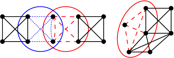
The conclusion of Lemma 13 does not hold when and . Following through the proof, the condition was only used in the second-last sentence. Thus we see that for , there is a single exceptional configuration: three triples with each pair meeting in a (distinct) vertex; we later refer to this as a ‘clean -cycle’; see the first diagram in Figure 1.

3 Proof of Theorems 1 and 5
In this section we prove Theorem 5 and thus Theorem 1, which is the special case . We attempt to optimize the terminology for the case , speaking of (-)edges or just edges in the -uniform hypergraph , and hyperedges for the -uniform .
The overall strategy is similar to one employed by Bollobás and the author in [3]. Only at one point will we need to assume , so most of the time we assume only that . In essence, the idea is to test for the presence of each possible in (thus when ) one-by-one, each time only observing whether the is present or not, not which edges are missing in the latter case. It suffices to show that, at least on a global event of high probability (meaning, as usual, probability as ), the conditional probability that a certain test succeeds given the history is at least .
There will be some complications. A minor one is that we would like to keep control of the copies of ‘found so far’ by using rather than , since we don’t want to find too many copies. The solution to this is simple: if the conditional probability of a certain test succeeding given the history is , then we toss a coin independent of (and of all other coins), only actually testing for the copy of with (conditional) probability .
Another complication is that it will happen with significant probability that some tests that we would like to carry out have conditional probability less than of succeeding. Roughly speaking, as long as this happens times, we are ok. More precisely, each time this happens we toss a -biased coin to determine whether the relevant hyperedge is present in , and if so, our coupling fails. We will show that the coupling succeeds on a global event of high probability.
Turning to the details, fix . Let , and let denote the (-)edge-sets of all possible copies of in . Let be the event that , i.e., that the th copy is present. As outlined above, our algorithm proceeds as follows, revealing some information about while simultaneously constructing .
Algorithm 15.
For each from to :
First calculate , the conditional probability of the event given all information revealed so far.
If , then toss a coin with heads probability . If it lands heads, test whether the event holds. If so, declare the hyperedge corresponding to to be present in . If not, or if the coin lands tails, declare to be absent.
If , then toss a coin with heads probability , and simply declare to be present in if this coin lands heads. If this happens, our coupling has failed.
At the end, the hypergraph we have constructed clearly has the correct distribution for , so it remains only to show that the probability that the coupling fails is .
Suppose that we have reached step of the algorithm; our aim is to bound . In the previous steps, we have ‘tested’ whether certain (not necessarily all) of the events hold, in each case receiving the answer ‘yes’ or ‘no’. Suppressing the dependence on in the notation, let and denote the corresponding (random) subsets of . Then, from the form of the algorithm, the information about revealed so far is precisely that every event , , holds, and none of the events , , holds.
Let be the set of (-)edges ‘revealed’ so far. For let . Then what we know about is precisely that all edges in are present, and none of the sets , , of edges is present; see Figure 2. Working in the random (-)graph in which each (-)edge outside is present independently with probability , and writing for the event , we have
To estimate this probability we follow a standard strategy from the proof of Janson’s inequality, using a variation suggested by Lutz Warnke (see [13]). As usual, the starting point is to consider which events are independent of . In particular, let
Then
Now only involves the presence or absence (in ) of edges not in , so and are independent. Also, is an up-set, while is a down-set. Hence, by Harris’s inequality, . Thus,
Let
so and hence . Then, using the union bound, we have
| (2) |
Hence
| (3) |
where
| (4) |
which is of course random (depending, via and , on the information revealed so far). To prove Theorem 5 it suffices, roughly speaking, to show that almost always .
Proof of Theorem 5.
For the moment, we consider any fixed . We take for notational simplicity; it should be clear from the proof that follows that the arguments carry through when as long as is sufficiently small, meaning at most a certain positive constant depending on and .
For this we have . Hence the expectation of the degree of a vertex of is . Since the actual degree is binomial, it follows by a Chernoff bound that there is some such that whp every vertex of has degree at most , say. Let be the ‘bad’ event that some vertex of , the final version of the hypergraph constructed as we run our algorithm, has degree more than , so .
Let be the ‘bad’ event that contains an avoidable configuration, as defined in Section 2. By Lemma 12 we have .
Consider some , which will remain fixed through the rest of the argument. As outlined above, we condition on the result of steps of our exploration; we will show that if and the hyperedge corresponding to is present in (the only case where the coupling fails), then holds. The graph of ‘found’ edges is a subgraph of the (-)graph formed by replacing each hyperedge of by a . Hence , and we may assume that
| (5) |
since otherwise holds.
Let us consider a particular , and its contribution to . Let be the (-)graph with vertex set in which we include a (-)edge if it is in . Then the contribution is exactly , where . For example, in the situation illustrated in Figure 2, with corresponding to the red on the left, consists of two edges, one from and one (the curved blue dotted edge) from ; thus .
Crudely, is at least the number of edges of (the complete -graph on ) not contained within the vertex set of any component of . Suppose first that has at least two components, and let their orders be , ; this numbering will be convenient in a moment. Note that . Note also that (by definition of ), and intersect in at least one edge. Thus has at least one (-)edge and so at most components, i.e., .
Given the constraint , with each , by convexity the sum of is maximized when and . Thus
We next consider how many may lead to a configuration of this type, specifically, one where has components. Note that is formed of edges in , a (-)graph of maximum degree at most , and includes at least one vertex of a given set of size . It follows that there are at most
| (6) |
such choices: choices for an initial vertex in ), then at most choices each time we start a new component other than the first, and (crudely) at most choices for each subsequent vertex within a component. Hence the contribution of such terms ( having components) to is at most
A fairly standard calculation shows that this is (in fact, bounded by a small negative power of ); indeed, the power of in a given term of the sum is at most plus
and this function of is strictly convex on , zero for and negative for ; it follows that it is negative for .
It remains only to treat the case where is connected. There are at most terms of this form (by the argument for (6) with ), so the contribution from those with is at most . This leaves the case where , i.e., where . Such contribute exactly , so we have shown that if does not hold, then
| (7) |
where
In particular, when does not hold and , we have . Thus, recalling (3), we may choose so that in such cases , and our coupling cannot fail at such a step.
Let us call step dangerous if . Note that in any such step we have , since if we do have , then but (since ) we have , giving a contradiction. In a dangerous step, we toss a new -probability coin to determine whether the hyperedge corresponding to is present in . If it is, we call step deadly. Our coupling fails if and only if there is some deadly step . To complete the proof it thus suffices to show that if any step is deadly, then holds. If step is deadly, then every (-)edge in lies within some hyperedge of , but the hyperedge corresponding to is not present in (since ). In this case, using (only now) the condition , by Lemma 13 contains an avoidable configuration, i.e., holds. Thus, if our coupling fails, holds, an event of probability . This completes the proof of Theorem 5. ∎
4 The triangle case
In this section we prove the following result, a weakening of the (missing) case of Theorem 1. The result itself is of no relevance, since it is superseded by Annika Heckel’s stronger result [7], but the proof method may perhaps be. In particular, we will use the same idea in a more complicated context in Section 5, and it seems easier to introduce it in the present simple case.
Theorem 16.
There exists a constant such that, for any , the following holds. Let be constant, and let . Then we may couple the random graph with the random hypergraph so that, whp, for every hyperedge in there is a copy of in with the same vertex set.
The proof of Theorem 1 given in the previous section ‘almost’ works for . The only problem is the unique exception to Lemma 13, a ‘clean’ hypergraph 3-cycle; an -uniform hypergraph is a clean -cycle if it can be formed from a graph -cycle by adding new vertices to each edge, with the added vertices all distinct; see Figure 1. (We extend the definition to , when it simply means two hyperedges sharing exactly vertices.)
Remark 17.
Simply by ‘skipping over’ dangerous steps, for the proof of Theorem 1 shows the existence of a coupling between and , , so that whp for every hyperedge of which is not in a clean 3-cycle (i.e., almost all of them) there is a corresponding triangle in .
Alternatively, as claimed in Theorem 16, we can avoid leaving out any hyperedges of , at the cost of decreasing its density by a constant factor.
Proof of Theorem 16.
We are given a constant . Fix another constant such that
| (8) |
(Of course always works; in Section 5 other choices will be useful.) In the previous section we examined the random graph according to Algorithm 15, checking copies of for their presence one-by-one. Here, in addition to the random variables corresponding to the edges of , we consider one /-random variable for each of the possible copies of , with . We take the and the indicators of the presence of the edges in to be independent. We think of the as ‘thinning’ the copies of in , selecting a random subset. Note that should not be confused with the random variable describing the presence of the corresponding hyperedge in .
With , our aim will be to construct a random hypergraph with the distribution of so that for every hyperedge in there is a triangle in with . In other words, we try to embed (in the coupling as a subhypergraph sense) within the ‘thinned triangle hypergraph’ having a hyperedge for each triangle in with . This clearly suffices. But how does making things (apparently) harder for ourselves in this way help?
We follow the proof of Theorem 1 very closely. Consider the random (non-uniform) hypergraph , with edge set , i.e., an edge for each edge of , and a triple for each such that . We follow the same algorithm as before, mutatis mutandis333‘Changing what must be changed’, i.e., with the obvious modifications to the new setting., now examining rather than . At each step we check whether a given triangle is present ‘after thinning’, i.e., whether it is the case that and , where is the edge-set of . In other words, we test whether , where consists of the edges together with one hyperedge corresponding to ; an individual event of this form has probability . As before, we only record the overall yes/no answer, and write for the conditional probability of this test succeeding given the history. Because the (hyper)edges of are present independently, the argument leading to (2) carries through exactly as before, but now with the event that , and with the set of (hyper)edges of found so far. Noting that each triangle has its own ‘extra’ hyperedge, in place of (3) we thus obtain
| (9) |
where, as before,
The key point is that the first term in (9) contains one factor of (from the probability that ), while the second contains two, from the probability that .
We estimate exactly as before, leading to the bound (7), valid whenever does not hold. This time, let us call step dangerous if there are two (or more) distinct such that and are both contained in . If step is not dangerous, then from (7) we have , which with (9) gives
for large enough, where in the second step we used (8). Hence our coupling cannot fail at such a step.
As before, we call a dangerous step deadly if the hyperedge (now a triple) corresponding to is present in the random hypergraph that we construct. Our coupling fails only if such a step exists. As before, this implies that the simple graph corresponding to contains a triangle with edge-set , even though contains no triple corresponding to this triangle. We may assume that contains no avoidable configuration (otherwise holds). By Remark 14, it follows that contains a clean -cycle ‘sitting on’ . Similarly, contains a clean -cycle sitting on . Since we have that and both intersect in at least one edge. Hence there is a vertex common to and . It follows that and share at least one vertex. Since they are unicyclic and not identical, it easily follows that their union is connected and complex, and (since it has at most hyperedges) is hence an avoidable configuration. So does hold after all. Thus we have again shown that if our coupling fails, holds, an event of probability . ∎
5 Extension to -balanced graphs
In this section we state and prove an extension to certain -balanced (-uniform hyper)graphs , considering copies of in () rather than copies of . Our main focus is the graph case , but it turns out that the proof can easily be written to extend to with no changes. Still, we attempt to optimize the notation for , writing ‘(-)graph’ or sometimes just ‘graph’ for a -uniform hypergraph, as in Sections 2 and 3.
We shall write for and for throughout. Thus, recalling Definition 7,
Throughout we assume (otherwise is an edge and everything is trivial).
Note for later that if is strictly -balanced then is -connected: otherwise, it would be possible to write as , where and have at least two vertices and overlap in exactly one vertex. But then
a contradiction.
We will prove the analogue of Theorem 1 for nice graphs (see Definition 9), and the analogue of Theorem 16 for all strictly -balanced , in Theorem 18 below. At the end of this section we will use a variation of the method to prove Theorem 8. The coupling results are slightly awkward to formulate, since we cannot directly encode copies of by an -uniform hypergraph.
Let be a fixed (-)graph with vertices. By an -graph we mean a pair where is a finite set of vertices and is a set of distinct copies of whose vertices are all contained in . We refer to the copies as -edges. Equivalently, an -graph is an -uniform labelled multi-hypergraph, where each hyperedge is labelled by one of the possible copies of on , and we may have two or more hyperedges with the same vertex set as long as they have different labels.
For and we write for the random -graph with vertex set in which each of the
possible copies of (i.e., possible labelled hyperedges) is present independently with probability . Thus, when , an -graph is exactly an -uniform hypergraph, and .
Theorem 18.
Let be a fixed strictly -balanced -uniform hypergraph, , with and . Let . There are positive constants and such that if then, for some , we may couple and such that, with probability , for every -edge present in the corresponding copy of is present in . Furthermore, if is nice, then we may take .
In other words, in the same one-sided sense as in Theorem 1, and up to a small change in density, the copies of in (i.e., when ) are distributed randomly as if each was present independently.
The slightly awkward statement of Theorem 18 ‘does the job’ with respect to -factors, for nice , giving Theorem 10 as a corollary.
Proof of Theorem 10.
Fix a nice (-uniform hyper)graph with vertices and edges, and define as in the statement of the theorem, noting that is asymptotically the value of for which each vertex of (or ) is on average in copies of . Then for , say, the in Theorem 18 satisfies , where is defined in Theorem 2. Let be the random simple hypergraph obtained from by replacing each -edge by a hyperedge with the same vertex set (i.e., forgetting the labels) and removing any multiple edges. Then has the distribution of for
so we have , say, for large enough. Thus by Kahn’s Theorem 2, whp has a perfect matching. When this holds and the coupling described in Theorem 18 succeeds, for each hyperedge in the matching we find some copy of in with the same vertex set, leading to an -factor. The reverse bound is (as is well known) immediate: if then whp there will be vertices of not in any copies of . ∎
To prove Theorem 18 we will follow the strategy of the proof of Theorem 1 as closely as possible; the main complication will be in the deterministic part, namely the analogue of Lemma 13.
Given an -graph , let be the underlying -uniform multi-hypergraph, where we replace each -edge by a hyperedge formed by the vertex set of (i.e., forget the labels), and let be the simple (-)graph444From now on we mostly write just ‘graph’, only occasionally reminding the reader of the case . formed by taking the graph union of the copies of present as -edges in . We define avoidable configurations in (multi)-hypergraphs as before, now noting that two hyperedges with the same vertex set form an avoidable configuration (the nullity is ). We say that contains an avoidable configuration if does.
The next deterministic lemma describes how the union of copies of can create an ‘extra’ copy .
Lemma 19.
Let be a -connected (-)graph with vertices, let be an -graph, and let be a copy of , not present as an -edge in , such that . Then either (i) contains an avoidable configuration, or (ii) contains a clean -cycle for some , with every edge of contained in some hyperedge in . Furthermore, if is nice, then (i) holds.
Proof.
We may assume that is minimal with the given property. Let its -edge-set be , so these are distinct graphs isomorphic to whose union contains . Let be the corresponding (-element) hyperedges, so , and let , a (multi-)hypergraph with hyperedges . Since is connected, it is easy to see that is connected. Suppose that has a pendant hyperedge, i.e., a hyperedge that meets only in a single vertex . Then, by minimality of , at least one edge of is included in , and at least one edge of is included in . In particular, includes at least one vertex other than in each of and . Since and meet only in , it follows that is a cut-vertex in , contradicting the assumption that is -connected.
So we may assume that has no pendant hyperedges. By minimality, every hyperedge of contributes at least one edge to , so .
If is complex, then is an avoidable configuration and we are done. Suppose not, so in particular has no repeated hyperedges. Certainly (since ), so cannot be a tree. Thus is unicyclic, and in fact it is a clean -cycle for some (see Figure 1). Note that . This completes the proof of the main statement. It remains only to deduce a contradiction in the case that is nice (so must have been complex after all).
So suppose that is nice. Let be the (-)graph555 is a graph even if . cycle corresponding to , so each hyperedge of consists of two consecutive vertices of and ‘external’ vertices. Then cannot contain any (-)edges within other than the edges of the -graph . Since is -connected, it is not a subgraph of , so contains a vertex outside . Assume without loss of generality that . Let and be the vertices of in . Then , a union of two (-)graphs whose vertex sets intersect in . Since is 3-connected, it follows that , so in fact these two sets of vertices are the same. Now every contributes at least one edge to . For this edge can only be , so we conclude that and that (so also ). Hence it is possible to transform into an isomorphic graph by adding one edge and then deleting one edge. Since is nice, this is impossible. ∎
Definition 20.
Let be an -graph and let be an -edge of . We say that is an extra copy of in meeting if
(i) is not present as an -edge in ,
(ii) all (-)edges of are present in , and
(iii) and share at least one (-)edge.
We write for the number of extra copies of in meeting .
The first two conditions above express that when we take the union of the copies of encoded by , then appears as an ‘extra’ copy of .
Definition 21.
Let denote the supremum of over all -graphs and , where contains no avoidable configuration.
Corollary 22.
If is -connected, then is finite. If is nice, then .
Proof.
The second statement is immediate from Lemma 19 and the definition of . For the first, let be an -edge of an -graph containing no avoidable configuration, and let be an extra copy of in meeting . Then, by Lemma 19, the hypergraph contains a clean -cycle for some , with each (-)edge of contained in a hyperedge of . Consider the hyperedge corresponding to . Then and share an edge , which must be contained in some hyperedge in . So shares at least two vertices with . If is not already a hyperedge of , it follows that is complex and thus an avoidable configuration, contradicting our assumptions. Hence is indeed a hyperedge of .
For any extra copy meeting we obtain a (unicyclic) witness as above. Each can be a witness for at most copies , since has vertices and so contains subgraphs isomorphic to . On the other hand, if contains two distinct witnesses then, since they share a hyperedge, their union is complex and has at most hyperedges, again contradicting our assumption that contains no avoidable configuration. ∎
We are now ready to prove Theorem 18.
Proof of Theorem 18.
We follow the proof of Theorem 1 (for the case nice) or Theorem 16 as closely as possible. In particular, we follow Algorithm 15 mutatis mutandis, testing copies of for their presence in (or for the -graph case) and simultaneously constructing a random -graph with the distribution of .
As before, it is convenient to assume that . Then , so the expected degrees in or its underlying hypergraph are at most . Writing for the (-)graph associated to , it follows as before that, for some , the event that any vertex has degree more than in has probability . Furthermore, by (a trivial modification of) Lemma 12, the event that contains an avoidable configuration has probability .
The core of the argument is exactly as before: we test the edge-sets of the possible copies for their presence in , or for , one-by-one. Our coupling only fails if the conditional probability that the -th test succeeds is smaller than , and the corresponding -edge is present in the random -graph that we are constructing; we write for this latter event. We aim to show that in this case, holds. We argue by contradiction, assuming that holds, but neither nor does; our aim is to show that then . Note that under these assumptions, and so .
The derivation of (3) did not use any properties of the , except to bound by in the last step. Thus we have
with defined as in (4), as before. For , we let be the (-)graph on formed by all (-)edges in that are also contained in , and write ; thus the contribution from this to is precisely .
We split the contribution to into two types, according to whether or not, writing
where, as before,
As before, we can split the sum according to the number of components and number of edges of , a non-trivial subgraph of . Since we assume , we obtain as before (see (6)) that
| (10) |
Suppose has components, with vertices and edges, respectively. Each component is a subgraph of , which is -balanced, so
| (11) |
In fact, is strictly -balanced, so we have a strict inequality if any is in the range . As before, contains at least one edge, so we cannot have all equal to one. Thus, when is disconnected, i.e., , we have a strict inequality in (11). When , by the way we split the sum we have , so we have a strict inequality. It follows that all terms in the sum in (10) are at most
so .
Turning to , if then the -edge is not present in (since , so by the definition of the algorithm we did not include as an -edge of ). On the other hand, since holds, the -edge corresponding to is present, and . Thus is an extra copy of in which (by definition of ) meets . We assume does not hold, so the number of possible such is at most . In conclusion,
If is nice then by Corollary 22, so and we are done. For general strictly -balanced , we know that is -connected, so is finite by Corollary 22. Thus we may bound by , say. Now we let and introduce extra tests (one per copy of ) as in the proof of Theorem 16. In this case we have , for , so (if neither nor holds), we have , as required. ∎
A slight variant of the proof above, with almost identical arguments but different parameters, yields Theorem 8.
Proof of Theorem 8.
Fix which is -balanced, but need not be strictly -balanced. Define , and as before. Pick a constant such that , and set
where the constant is chosen large enough that the random -graph (or rather, its underlying hypergraph), whp contains a perfect matching; such a constant exists by the result of Johansson, Kahn and Vu [8], and Theorem 2 gives an explicit value. Note that we may write where
We follow the proof of Theorem 18 above, in particular in the form with additional tests with probability as in the proof of Theorem 16. Since the expected degrees in are of order , we may take . As before, the event that has maximum degree more than , and the event that contains an avoidable configuration, have probability . To complete the proof we need only show that when neither nor holds, but the -edge corresponding to is included in , then . As before, we have , so it suffices to show that in this case .
Estimating as in the proof of Theorem 18, but this time not separating out the term, we have
where we used (11) (whose derivation only assumed that is -balanced) to bound by , and note as usual that the overlap graph contains at least one edge, so the number of components is at most . Now , while . It follows easily that the term dominates the sum above, so . Since , it follows that , completing the proof. ∎
Gerke and McDowell [6] consider multipartite multigraph analogues of the case of Theorem 8. Their main focus is the ‘nonvertex-balanced’ case, but they also prove a version for arbitrary losing a factor in the edge probability. The proof above extends mutatis mutandis to reduce this factor to when is -balanced. Since this is not our main focus, we only outline the details.
Let be a multigraph, which we will view as a graph with a positive integer weight on each edge. Let . As in [6], we will look for an -factor in a random graph where we first divide the vertices of into equally sized disjoint sets , and only consider copies of with each mapped to a vertex in . In [6], is a random multigraph, but their formulation is exactly equivalent to the following: we take all edges of to be present independently, and an edge between and has probability , where is the multiplicity of in . Then we look for a copy (restricted as above) of the simple graph underlying in this random graph .
The coupling arguments above translate immediately to this setting: we are still working in a product probability space, and if is a set of possible edges of , the probability that all are present is where now we count edges according to their multiplicity. Nothing else in the argument needs changing, except the hypergraph input. Let be the random -partite -graph where each of the possible hyperedges is present independently with probability . Then we need to know that if is at least some constant times , then whp has a complete matching. This statement follows easily from the Johansson–Kahn–Vu argument as presented by Frieze and Karoński [5], simply starting with a complete multipartite hypergraph and removing edges one-by-one, rather than starting with a complete hypergraph. This result also follows from Corollary 1.2 of Bal and Frieze [2], itself a consequence of a more general result needed there.
6 Open questions
The motivation for this paper was to understand, in the Johansson–Kahn–Vu context in particular, the relationship between the distribution of copies of in and the random hypergraph , . This rather vague question seems to make sense much more generally. The method used here works for up to for some . How large is this ? More interestingly, up to what is a result analogous to Theorem 1 true? It should break down when a typical edge of has a significant probability of being in a copy of , since then a significant fraction of the s in share edges, and these overlapping pairs are more likely in than in . Of course, this doesn’t rule out some other interesting relationship between and for even larger .
Turning to general graphs in place of , and looking for sharp results, say, with , one might ask what the right class of graphs is. The conditions in Theorem 18, and thus Theorem 10, are what makes the proof work, and are presumably more restrictive than needed. Strictly -balanced is a natural assumption, but even without this assumption there might still be a sensible way to relate copies of in to a suitable hypergraph, which might or might not be , depending on and on the value of .
In Theorem 1, one could ask how large a failure probability must be allowed in the coupling. The proof as given yields for some positive , coming from the probability that contains an avoidable configuration. But it could be that much smaller failure probabilities are possible. Also, what about comparing the distributions in some different way? In particular, looking for some two-sided sense in which they are close?
Finally, it would be interesting to know whether the simple proof of Theorem 16 given (in a very slightly different setting) by Kim [11], and outlined in Section 4.1 of the draft arXiv:1802.01948v1 of the present paper, can be extended to , perhaps by some kind of induction. It’s not at all clear whether this is possible, though.
Acknowledgements.
Part of this work was carried out while the author was a visitor at IMPA in Rio de Janeiro; the author is grateful to Rob Morris and to IMPA for their hospitality. The author would like to thank Annika Heckel for a helpful discussion of the hypergraph case, the referees for helpful suggestions, and the editors of Random Structures and Algorithms for their patience with the very late revision.
References
- [1] N. Alon and R. Yuster, Threshold functions for -factors, Combin. Probab. Comput. 2 (1993), 137–144.
- [2] D. Bal and A. Frieze, Rainbow matchings and Hamilton cycles in random graphs, Random Struct. Alg. 48 (2016), 503–523.
- [3] B. Bollobás and O. Riordan, Constrained graph processes, Electronic Journal of Combinatorics 7 (2000), #R18 (electronic, 20 pp.)
- [4] P. Erdős, On the combinatorial problems which I would most like to see solved, Combinatorica 1 (1981), 25–42
- [5] A. Frieze and M. Karoński, Introduction to Random Graphs, Academic Press (2016), 478 pp.
- [6] S. Gerke and A. McDowell, Nonvertex-balanced factors in random graphs, J. Graph Theory 78 (2015), 269–286.
- [7] A. Heckel, Random triangles in random graphs, Random Struct. Alg. 59 (2021), 616–621.
- [8] A. Johansson, J. Kahn and V. Vu, Factors in random graphs, Random Struct. Alg. 33 (2008), 1–28.
- [9] J. Kahn, Asymptotics for Shamir’s Problem, preprint (2019), arXiv:1909.06834v1
- [10] J. Kahn, Hitting times for Shamir’s problem, Trans. Amer. Math. Soc. 375 (2022), 627–668.
- [11] J. H. Kim, Perfect matchings in random uniform hypergraphs, Random Struct. Alg. 23 (2003), 111–132.
- [12] M. Krivelevich, Triangle factors in random graphs, Combin. Probab. Comput. 6 (1997), 337–347.
- [13] O. Riordan and L. Warnke, The Janson inequalities for general up-sets, Random Struct. Alg. 46 (2015), 391–395.
- [14] A. Ruciński, Matching and covering the vertices of a random graph by copies of a given graph, Discrete Math 105 (1992), 185–197.
- [15] J. Schmidt and E. Shamir, A threshold for perfect matchings in random d-pure hypergraphs, Discrete Math 45 (1983), 287–295.