Dynamical regularities of US equities opening and closing auctions

Abstract

We first investigate the evolution of opening and closing auctions volumes of US equities along the years. We then report dynamical properties of pre-auction periods: the indicative match price is strongly mean-reverting because the imbalance is; the final auction price reacts to a single auction order placement or cancellation in markedly different ways in the opening and closing auctions when computed conditionally on imbalance improving or worsening events; the indicative price reverts towards the mid price of the regular limit order book but is not especially bound to the spread.

keywords: auctions; US equities; linear response; imbalance; liquidity

1 Introduction

Many equity exchanges use auctions to define meaningful opening and closing prices associated with substantial liquidity and to decrease price volatility near opening and closing times. Despite their practical importance and the fact that the relative volume traded at the opening and closing has been steadily growing, as show below, these auctions have not attracted much work recently, as the attention of the community has focused on price discovery issues and intraday dynamics. A central question in the literature is for example the usefulness of auctions. One criterion is that of market quality, defined for example as the volatility of the price and bid-ask spreads just after the opening auction or just before the closing auction. Generally, auctions improve market quality (see e.g. Pagano and Schwartz (2003); Chelley-Steeley (2008); Pagano et al. (2013)).

Our focus is rather on the auctions themselves and particularly on the pre-auction periods. Papers closely related to ours are only a handful. Gu et al. (2008) find a power-law tailed density of the position order placement on both sides of reference prices in the Shenzhen Stock Exchange; Kissell and Lie (2011) report the average fraction of the auction volumes with respect to the total daily volume and their dependence on special days (month end, quarter end, etc.) and on the capitalization of the assets of US equities. Gu et al. (2010) report that the average density of the auction limit order book on both sides of the final auction price is well fitted by an exponential distribution and compute the persistence fluctuation properties of the order size in the Shenzhen Stock Exchange. More recently, and more in line with our paper, Boussetta et al. (2016) study the French Stock exchange and find that different kind of market participants enter the pre-auction periods at markedly different times, the slow brokers acting first, while high-frequency traders tend to be active nearer the end of auctions. In the same vein, Bellia et al. (2016) show how and when low-latency traders (identified as high frequency traders) add or remove liquidity in the pre-opening auction of the Tokyo Stock Exchange. Lehalle and Laruelle (2018) devote part of a chapter to auctions in a spirit close to ours, in particular regarding typical daily activity patterns. Finally, Challet (2019) shows that in Paris Stock Exchange, the antagonistic effects of accelerating event rate near the auction time and the decrease of the typical indicative price volatility cannot fully explain the observed diffusion properties of the indicative price, which is likely due to strategic behavior.

This paper is organized as follows: we first determine the distribution of the volumes of matched orders at both auction ending times. We then find rules of thumb to estimate opening and closing volumes from daily data. Finally, we examine the dynamics of the indicative price, imbalance, and matched volume. We show in particular that the reaction of the final auction price to the placement or cancellation of an order is markedly different in the opening and closing auctions, and that the indicative auction prices are mostly under-diffusive, especially during the pre-closing auction period. Finally, we relate the dynamics of the indicative price to that of the limit order book: although the mid price does attract the indicative price, the latter fluctuates rather much and is not specially bound to be in the spread, which, we argue, is due to the sparseness of the auction order book.

2 Data

Each exchange follows its own auction rules and pre-auction information dissemination procedure. The basic principle of all auctions however is the same: traders may submit market orders for the auction (buy/sell a given volume at any price), or limit orders (buy/sell a given quantity at a given price) which may be valid either for the auction only or stay in the open-market order book after the auction if they are not matched. Finally, the matching price is fixed so as to maximize the matched volume; if such price is not unique, the one closest to the previous close price is selected.

What kind of orders and when they may be sent, however, significantly differs between NYSE Arca (henceforth shortened to ARCA), NYSE and NASDAQ. For example, during the closing auction on ARCA, limit and market auction orders (known as LOC and MOC, respectively) may be sent until one minute before the auction time, then during the last minute, only orders reducing the imbalance are accepted. For NASDAQ, the cut-off time for LOC/MOC orders has been reduced to 5 minutes in October 2017. Cut-off time is 10 minutes before the closing auction for NYSE, which adds discretionary quotes (D-quotes) that may override imbalance-reducing orders; they are added five minutes before the auction time, may be submitted or modified up to 10 seconds before auction time, and be cancelled at any time. While these differences have no direct influence on the measure of matched volumes, they are likely to change the dynamic properties near the auction times. Because only ARCA continuously disseminates information, we cannot document these differences.

We use three data from three different sources:

1. Individual matched order sizes. For assets traded on ARCA, our Thomson-Reuters Tick History data set includes an order-by-order breakdown of auction volumes from 2009-02-10 to 2014-07-01. To fix notations, $v_{\alpha,k,d}^{x}$ is the volume (in shares) of the $k$-th matched order for asset $\alpha$ on day $d$ for auction $x\in\{\text{open,close\}}$. This dataset contains 16,165,407 orders.

2. Daily matched volume for each auction, for the three exchanges, gathered from the proper flag of Thomson-Reuters tick-by-tick trades data. We denote by $V_{\alpha,d}^{x}$ the total matched volume of auction $x$ of security $\alpha$ on day $d$. By definition, $V_{\alpha,d}^{x}=\sum_{k=1}^{N_{\alpha}^{x}(d)}v_{\alpha,k,d}^{x}$ where $N_{\alpha}^{x}(d)$ is the number of matched orders at the $x$ auction of asset $\alpha$ on day $d$. We shall also denote the auction price by $p_{\alpha,d}^{x}$ This data set encompasses 4712 US assets from 2010-01-01 to 2016-11-30, which amounts to 3,125,786 open and close auctions (each), among which 179,669 (6%) for ARCA, 446,396 (14%) for NASDAQ and 2,499,721 for NYSE (80%).

3. Finally, we gathered the real-time information disseminated by the three exchanges from 2016-09-28 to 2018-01-12 for 1076 assets. This information consists in the indicative price $\pi_{\alpha,d}^{x}(t)$, the current matched volume at that price $W_{\alpha,d}^{x}(t)$, and the current imbalance $I_{\alpha,d}^{x}(t)$, defined as the sum of the market order imbalance and of the limit order imbalance at the indicative price. While NYSE and NASDAQ only publish a few snapshots of these quantities per auction, ARCA disseminates up to a few thousand updates for each auction on each day. The ARCA dataset contains 47,246,490 updates for 58 tickers. Our data provider has a limit of about 4 updates per second; while this is sufficient in most cases, it becomes insufficient near the auctions times of very liquid assets such as SPY.

3 Matched volumes

We first focus on fairly stylized properties of auctions volumes and then turn to a more refined analysis of the pre-auction dynamics: indicative price, volume, activity rate and relationship with the regular limit order book.

3.1 Single order properties

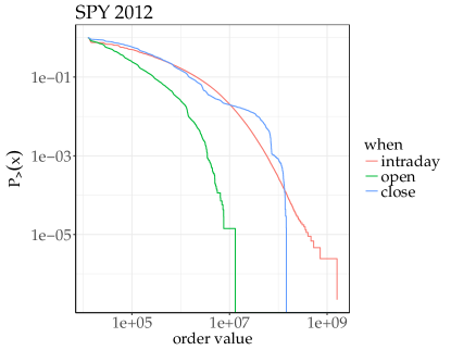
Figure 1: Reciprocal empirical distribution function of the value of all the trades of open auctions, close auctions and intraday trading of two of the most liquid assets traded at ARCA during 2012.

Figure 1 shows the reciprocal empirical distribution functions of the transaction values of matched orders defined as $p_{\alpha,d}^{x}V_{\alpha,d}^{x}$ at both auctions, together with that of the open-market transaction values, for SPY and GLD, two of the most liquid assets traded on ARCA for the whole 2012 year. The distributions of the opening and closing auctions are clearly much more affected by truncations than that of the open-market transactions, and the opening auction more than the closing auction. They reflect, to some extent, the fact that the typical total volume is larger at the closing auction than at the opening auction.

This raises the question of the nature of the matched orders distribution of a single day: does the heavy-tailed nature of $P(p_{\alpha,d}^{x}V_{\alpha,d}^{x})$ come from daily fluctuations or from the distribution of single order value distributions themselves? Whether the latter have heavy tails may be assessed by fitting it with an exponential and a log-normal distributions and using the Vuong closeness test (Vuong, 1989). We perform it for each day and each auction with more than 100 matched orders, which amount to 29168 auctions. There is overwhelming evidence of the presence of heavy tails, corresponding by convention here to small p-values: about 92.8% of the auction distributions have a p-value smaller than 0.01, while only 0.1% have a p-value larger than 0.99. Next, we check what distribution may best describe the tails. We use the method of Clauset et al. (2009); Alstott et al. (2014) to determine the best starting point of a power-law tail and then investigate how a fit of that tail with a power-law compares with log-normal, exponential, and truncated power-law distributions. Figure 2 plots the density of p-values of a Vuong test between a power-law and the other candidates, computed for each day, each stock and each auction with more than 100 matched orders. Expectedly, it confirms the heavy-tailed nature of the tails. Finally, it shows no real difference between a power-law and a log-normal distribution, while a truncated power-law does not bring a substantial improvement on average.

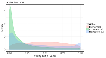
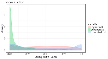
Figure 2: Tails of the individual matched order volume distribution, for each day, each asset assessed by the p-values of the Vuong test of a power-law against log-normal, exponential and truncated power-law.

3.2 Opening, closing and daily volumes

The total daily volume for a given asset is freely available in contrast to auction volumes. Thus, we endeavor here to find a rule of thumb to infer the opening and closing auction volumes from daily data only. Let us focus on the ratios of auction volumes to total daily volume, denoted by

$$\rho_{\alpha,d}^{x}=\frac{V_{\alpha,d}^{x}}{V_{\alpha,d}^{\text{total}}},$$

where $V_{\alpha,d}^{\text{total}}$ is the total volume exchanged during day $d$, including both auctions, OTC transactions, and outside regular trading hours transactions. We start with averages over the period 2010-01-01 to the end of the dataset. Figure 3 plots the densities of $\log_{10}(\rho)$ for the three exchanges, each day and each asset. The largest difference between the open and close is observed in the NYSE exchange, possibly because it is not fully automated. For example, the opening auction ending time is not fixed and may happen a few minutes after the opening of the exchange itself. Remarkably, the close of the NYSE has by far the largest percentage of volume with respect to the other exchanges. NASDAQ has the least variability between assets and auctions. We also plot in the same figure the densities of the median logarithmic ratio asset by asset in order to assess the intrinsic diversity of these ratios between the assets. Once again the variability of the volume ratio between asset of ARCA is the largest one. The least asset variability for the opening auction is found in NASDAQ, while NYSE takes the crown for the closing auction volume fraction, closely followed by NASDAQ. This yields simple rules of thumb for all the assets: between 2010 and 2016, 12% of daily volume is exchanged at the close of NYSE, 3% the opening of NASDAQ and 7% at the close of NASDAQ. The densities of ARCA volume ratios are too wide to be summarized by simple rules of thumb.

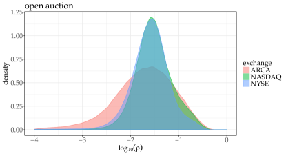
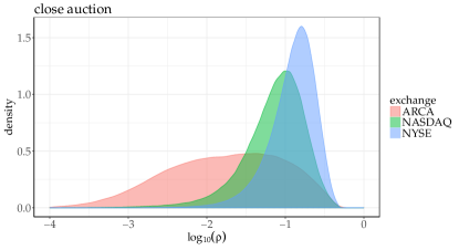
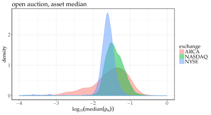
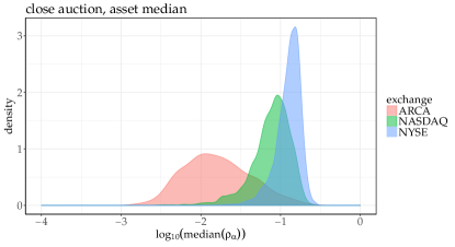
Figure 3: Upper plots: density of the logarithmic ratio of the auction volumes to the total daily exchange volume $\rho_{\alpha,d}^{x}=\frac{V_{\alpha,d}^{x}}{V_{\alpha,d}^{\text{total}}}$ for each day and each asset, split by exchange. Lower plotw: density of the asset median logarithmic ratio, split by exchange.

$\log_{10}\rho_{\alpha,d}$	ARCA	NASDAQ	NYSE
open	$-1.72\pm 1.24$	$-1.51\pm 0.79$	$-1.61\pm 0.90$
close	$-1.78\pm 1.47$	$-1.15\pm 0.82$	$-0.91\pm 0.60$

$10^{\text{mean}(\log_{10}\rho)}$	ARCA	NASDAQ	NYSE
open	$0.019$	$0.031$	$0.024$
close	$0.017$	$0.071$	$0.12$

Table 1: Left table: mean and two standard deviations of the volume ratio per auction $\log_{10}\rho_{\alpha,d}$, split by exchange. Right table, typical volume fraction $10^{\text{mean}\log_{10}\rho_{\alpha}}$

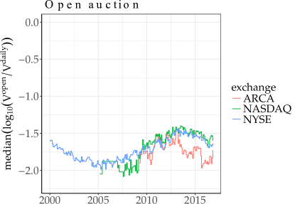
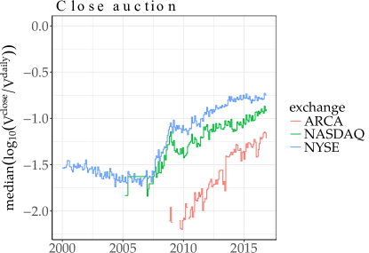
Figure 4: Monthly median of the volume exchanged at an auction divided by the total daily volume; months with less than 100 assets have been filtered out; left plot: open auction, right plot: close auction.

This, however, is a static picture determined over more than 7 years. The fraction of volume exchanged at auctions is not roughly constant. Figure 4 plots the monthly median fraction of the auction volume divided by the total daily volume as a function of time (months with less than 100 assets have been filtered out which essentially removes the beginning of the time-series for ARCA and NASDAQ. It turns out that the median closing auction fraction has been steadily increasing for all exchanges, except for NYSE for which this quantity has plateaued in 2015, while the opening auction fraction has been decreasing since 2012, on average. One should note once again that the median is taken over all assets of a given exchange, and thus this plot does not apply to a given asset in particular, as the difference between assets may be quite large. In other words, inference should be performed asset by asset, which is beyond the scope of this paper.

4 Pre-auction dynamics

Exchanges disseminate pre-auction information about indicative price, current imbalance at that price and matched volume at that price. The frequency of update is quite variable: ARCA gives away the most frequent information, NYSE gives updates with increasing frequency as the auction nears, while NASDAQ publishes the smallest amount of information (only one update before the open). We thus shall focus on assets traded on ARCA and briefly on those traded on NYSE. We remind the notations: the imbalance of asset $\alpha$ at auction $x$ on day $d$ at time $t$ is denoted by $I_{\alpha,d}^{x}(t)$, the currently matched volume by $W_{\alpha,d}^{x}(t)$, and the indicative price by $\pi_{\alpha,d}^{x}(t)$.

4.1 Typical activity

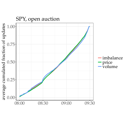
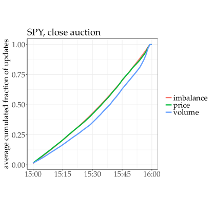
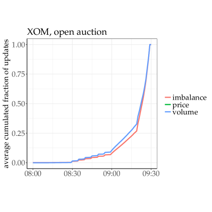
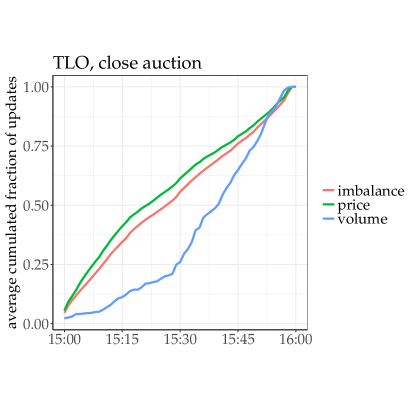
Figure 5: Average fraction of cumulated number of events as a function of the time for SPY (ARCA), XOM (NYSE) and TLO (ARCA).

Let us first investigate the typical update patterns. For each asset and day, we measure at fixed time resolution (1 minute) the ratio between the number of updates up to time $t$ (in minutes) and the total number of updates for that particular day, and then compute the average of this quantity over all the days. By definition, this quantity increases monotonically.

In the NYSE, updates to each quantity are disseminated at fixed times with a strongly accelerating pattern (convex cumulated number of updates), as can be seen for XOM in Fig. 5. Update times of ARCA on the other hand are not fixed, which allows one to quantify asset by asset how the activity unfolds, on average. Intuitively, one would expect that the activity increases as the time of the auction nears. This is the case in other kind of auctions with fixed ending times, such as on eBay (see e.g. Borle et al. (2006)). Indeed, in auctions, sending a non-cancellable bid reveals some information about one’s intentions. However, the fact that activity may concentrate just before the time of the auction is not always related to strategic behavior. Indeed, human beings tend to prefer to act just before a deadline in less competitive contexts, such as sending an abstract to a conference, or paying its fee (Alfi et al., 2007, 2009). Delaying one’s order submission minimizes the risk of divulging directional information too early. Another possibility to avoid leaking too much information for the traders is to synchronize their actions at fixed times so that individual actions are lost in a multitude of orders, as it is the case for example at 8:30 for SPY (see below), and, to much larger extent in Paris Stock Exchange (Challet, 2019).

Most practitioners however would be more interested in the evolution of the typical fraction of the indicative matched volume divided by the final auction volume at a given time. Here, we compute for asset and each day the fraction $W_{\alpha,d}^{x}(t)/V_{\alpha,d}^{x}$ every minute and compute its average and median for each asset. Figure 6 plots this quantity for SPY and TZA. During the opening auction, one generically notices an acceleration of the matched volume which is much larger than that of the number of volume updates, especially after 9:15. This implies that larger orders are submitted closer to the auction ending time, which is consistent with people trying to avoid having too much direct impact on the indicative price since the matched volume increases as a function of time. One also notices that a sizeable fraction of the daily volume auctions are submitted at or near 8:30 and 8:45 for both assets. Nevertheless, these two tickers have been chosen to illustrate the lack of universality across assets. Indeed, TZA clearly shows that during some days, a large fraction of the auction is cancelled just before the closing auction, but that this is not systematic as the median fraction does not exceed 1. This also happens for other assets either at the opening or closing auctions. According Bellia et al. (2016), cancellations near auction ending time are mostly due to high-frequency traders. The behavior of this quantity on US exchanges is markedly different from that of Paris Stock Exchange for which Challet (2019) finds that the number of events increases as a power-law until the auction time.

While SPY has a clearly accelerating, convex average matched volume ratio as a function time, we systematically investigated this pattern asset by asset by fitting polynomials of the first and second degree to $W_{\alpha,d}^{x}(t)/V_{\alpha}^{x}(d)$, and computing their respective Akaike Information Criterion (AIC). Using once again the Vuong ratio test, one finds that a linear fit is favored in 3% for the assets at the opening auctions, and none at the closing auction at the 5% level; reciprocally, a second degree fit is better than a linear fit in 64% for both auctions, the remaining 33% being undecidable. Among these 64% of assets, 75% have a convex, accelerating behavior at opening auctions, and 89% at closing auctions.

Finally, one may be interested in the typical time at which the average indicative matched volume reaches a given percentage of the auction volume. For each asset traded on ARCA, we computed the median time (over the days) of the time at which 50% of the total auction volume was matched and found two peaks centered at 8:30 and 8:55 for the opening auction, and a large peak centered at 15:35 for the closing auctions.

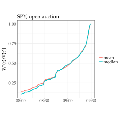
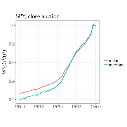
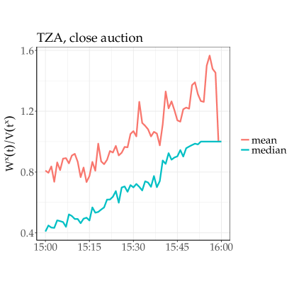
Figure 6: Average and median fraction of matched volume and total auction volume as a function of the time for SPY and TZA, traded on ARCA.

4.2 Mean-reversion and sub-diffusive prices

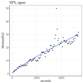
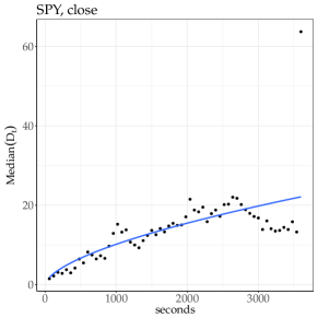
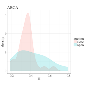
Figure 7: Left and center plots: median square dispersion of the indicative auction price with respect to the auction price versus the time remaining until the auction, together with a power-law fit (Hurst exponent $H\simeq 0.45$ for the opening auction and $H\simeq 0.23$ for the closing auction. Right plot: histogram of the Hurst exponent $H$ for all tickers of ARCA from fits whose p-values associated with $H$ are smaller than 0.001.

Focusing on ARCA data, we first check if the indicative price behaves as a standard Brownian motion, or if the existence of a final auction time and the fact that the activity and matched volume increases steadily have an influence of the indicative price fluctuation patterns. More precisely, we measure how the squared difference between the indicative match log-price $\log\pi_{\alpha,d}^{x}(t)$ and the final auction log-price $\log p_{\alpha,d}^{x}(t^{x})$, rescaled by daily variance of the indicative price log returns, scales with $\tau=t^{x}-t$ by defining

$$D(\tau)=\frac{\log(p_{\alpha d}^{x}(t^{x})/\pi_{\alpha,d}^{x}(t)){}^{2}}{\text{var}([\log(\pi_{\alpha,d}^{x}(t)/\pi_{\alpha,d}^{x}(t-1))])}$$ (1)

Generally, $D(\tau)\propto\tau^{2H}$ where $H$ is the Hurst exponent. Diffusive processes have $H=1/2$, whereas under-diffusive processes correspond to $H<1/2$. Note that we normalize by the variance of the indicative price log returns of each day, so as to be able to define $D$ as an average over days in a meaningful way. We first filter out single auctions with less than 50 price updates. We then discretize $\tau$ into slices of 1 minute, compute the median of $D$ of the days for each slice $\tau$, and perform a non-linear fit $\text{median }D(\tau)=a\tau^{2H}$ (removing $\max_{\tau}\text{median }D(\tau)$ for the sake of robustness). The left and middle plots of Fig. 7 show an example of the dependency of $D$ on $\tau$ for the asset with the largest number of updates (SPY); the peak at 08:30 is due to the fact that many traders submit auction orders around that time, whose effective imbalance may considerably shift the indicative match price, usually followed by an opposite jump or gradual relaxation. The right-hand-side plot displays the density of $H$ over all the assets with enough data on ARCA (we only kept fits whose p-values associated with $H$ are smaller than 0.001). We find that the indicative price of the opening auction is sub-diffusive for 73% of the assets for the opening auction and 93% of the assets for the closing auction.

The sub-diffusive property probably has several causes. First, diffusion is computed backwards from the auction ending time, thus the typical event rate decreases as the time-to-auction increases, which mechanically leads to sub-diffusion, provided that the immediate impact per event stays roughly constant. Challet (2019) discusses this hypothesis in greater details with data from Paris Stock Exchange, in which the analysis is simplified by simple scaling laws of both the number of events and the typical indicative price change as a function of time, and concludes that mechanistic effects alone cannot account for the observed price behavior, which confirms the importance of strategic behavior. Since no such scaling law holds in our data, we cannot replicate this result for US equities.

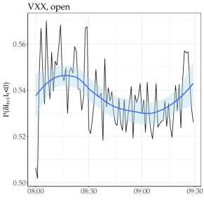
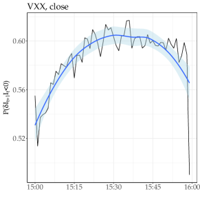
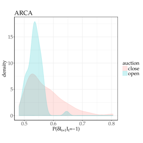
Figure 8: Left and middle plot: average probability that a new event reduces the imbalance as a function of time for VXX and both opening and closing auction. Right plot: histogram of the average over days for each ticker of that probability.

Indeed, another cause of sub-diffusion comes from the way new orders tend to cancel the current imbalance on average. In other words, a strategic way of placing new auction orders consists in waiting until the imbalance sign is the opposite from that of one’s intentions and only then sending one’s orders. Defining the imbalance difference of a new event (new order or cancellation) by $\delta I_{t+1}=I_{t+1}-I_{t}$, this strategic behavior can then be characterized by $P[\text{sign }(I_{t+1}\times\delta I_{t})=-1]$. Note that this also includes order cancellation, which is much rarer than order placement and will be thus neglected here. Figure 8 shows the evolution of this conditional probability as a function of time for VXX, which is representative of many other assets whose main exchange is ARCA: this probability is smaller for the opening auction than the closing auction for about 95% of the assets. In addition this probability shows a clear maximum for the closing auction at around 15:30. Some other assets display an increase of this probability in the last few minutes before the auctions (SPY, for one). In passing, note that this probability is about 1/2 for SPY during the opening auction, and about 0.53 (and roughly constant) during the closing auction, which is probably due to the fact that our data feed cannot keep up with the event rates of this asset.

4.3 Response functions

A more refined way to characterize the dynamics of pre-auction periods consists in measuring how the final auction price reacts to a given type of event as a function of the time remaining until the auction. For example, is the average response of the auction price to a new buy order placed at time $t$ positive or negative? In open-market order books, the answer is intuitive enough. Auctions are different at least for two reasons. First, as there is no trade before the auction ending time, real impact is not immediate. Second, sending an order to an auction reveals some information about one’s intentions, thus there is a clear strategic aspect to the time of order submission or cancellation. In other words, early orders may trigger a different response than later ones simply because the traders who submit the former have different strategies or expectations than the latter ones and may or may not cancel some of their orders before the auction ending time, in line with Boussetta et al. (2016).

Let us first derive the nature of several kinds of events from the sign of the changes of indicative imbalance and matched volume. Table 2 lists the three kind of event that may be inferred from out data feed. Note that this kind of determination becomes imprecise if the fraction of missing updates becomes substantial.

$\delta I$	$\delta M$	event
$>0$	$>0$	new buy order
$<0$	$>0$	new sell order
any	$<0$	cancellation or limit order price revision

Table 2: Type of event depending on the change of imbalance, matched volume and match price.

Inspired by Bouchaud et al. (2006), we define the linear response function of the auction price to a new order, for a given asset $\alpha$, at given update time $t_{i}$, as

$$R_{\text{$\alpha$,+}}(t_{i})=\text{median}\left(\epsilon_{\alpha,d}(t_{i})\left[\log p_{\alpha,d}^{x}-\log\pi_{\alpha,d}^{x}(t_{i})\right]|\delta W_{\alpha,d}(t_{i+1})>0,\delta I(t_{i+1})\neq 0\right)_{i,d},$$ (2)

where $\epsilon_{\alpha,d}(t_{i})$ is the sign (1 for buy and -1 for sell orders) of the $i-$th order placed during day $d$ for auction $x$ at time $t_{i}=t$ and asset $\alpha$, and $p_{\alpha,d}^{x}$ is the auction of price at time $t_{x}$. The idea is that on average a new buy order pushes the auction price $p^{x}$ in direction opposite to that of a sell order, hence the multiplication of the price difference by the sign of the new order. The same kind of response function can be defined for order cancellations, which occur when the matched volume decreases ($\delta W<0$), which we denote as $R_{\text{$\alpha$,-}}$. Figure 9 shows that early new orders have a definitely positive impact on average, while cancellation has an opposite effect.

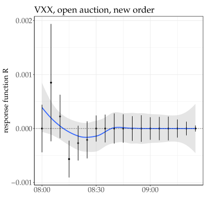
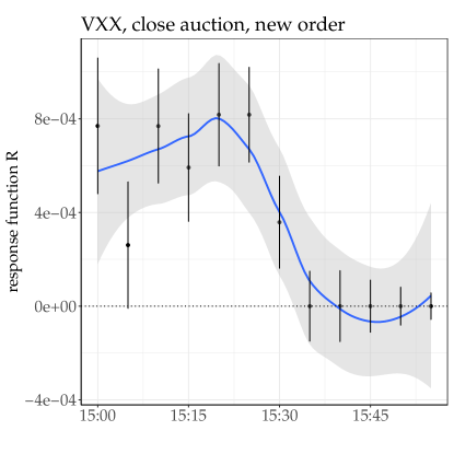
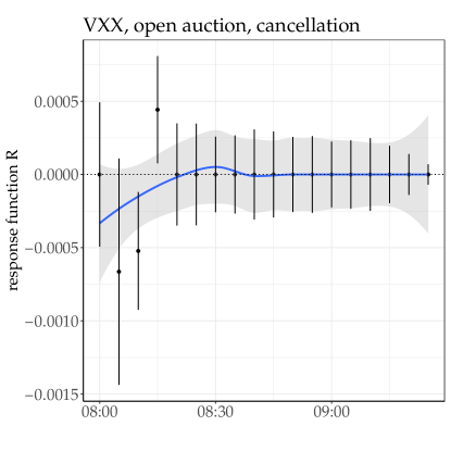
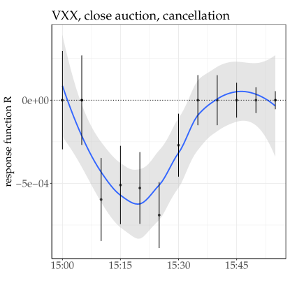
Figure 9: Median response functions of a new order (left plot) and order cancellation during the auctions of VXX. Error bars correspond to two standard deviations.

It is most revealing to discriminate between events that worsen or improve the current imbalance. Practically, one computes a response function for each value of $\text{sign }I(t)\times\delta I(t+1)$. This yields a much richer picture, as show by Fig. 10. For many assets, there is a clear maximum of the conditional response function of a new imbalance-worsening order. Once again, cancellations have globally opposite effect. Most surprising at first is the fact that for many assets, the sign of the conditional response function reverts between the opening and the closing auctions. This emphasizes the fundamental difference between the two auctions. While we cannot provide a definitive explanation for this phenomenon, we believe that it is mostly due to the fact that active trading takes place during the closing auction, while much fewer trades take place during the opening auction of US equities. Finally, note that the response functions of different assets are quite different, which reflects the fact that the typical population of traders may vary much from asset to asset. As a consequence, there is no such thing as the average response function. This is also the case for the response functions of open market limit order books, which depends for example on the exponent of the autocorrelation of market order signs (Bouchaud et al., 2006), which in turn depends on the market participant population (Toth et al., 2012).

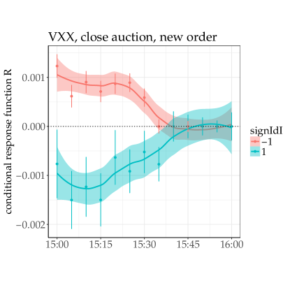
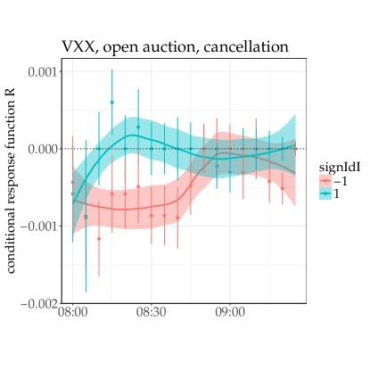
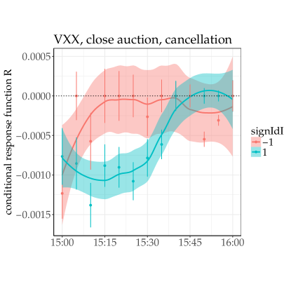
Figure 10: Response functions of a new order (left plot) and order cancellation conditional on an increase ($\text{sign }I_{t}\delta I_{t+1}=1$) or a decrease ($\text{sign }I_{t}\delta I_{t+1}=-1$) of the absolute total imbalance during the pre-open auctions of VXX. Error bars correspond to two standard deviations.

4.4 Indicative price and regular limit order book

Characterizing the dynamics of the indicative price also requires to study its interplay with the best prices of the regular market order book. First, some mathematical notations: $a(t)$ is the best ask price, $b(t)$ the best bid price, $m(t)=[a(t)-b(t)]/2$ the mid price and $m_{w}(t)=\frac{v_{a}a-v_{b}b}{v_{a}+v_{b}}(t)$ the mid price weighted by the respective available volumes ($v_{a}$ and $v_{b}$) at the best prices. Intuitively, the indicative price $\pi$ must be related in some way to the mid price, since both these price are proxies of the price discovery of the same asset, although in markedly different ways.

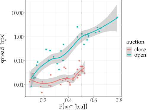
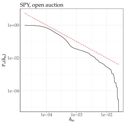
Figure 11: Left plot :median spread in bps versus the fraction of time spent in the spread by the indicative auction price for the 35 most active assets. Right plot: reciprocal cumulative distribution function $P_{>}(\delta_{m}=|\pi-m|/m)$ for the open auctions of SPY; the dotted red line is $\propto 1/\delta_{m}$ and is for eye-gudiance only.

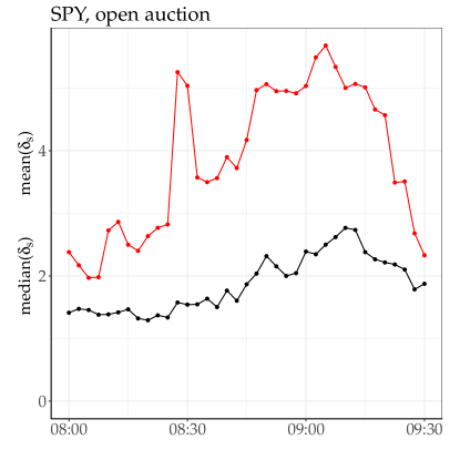
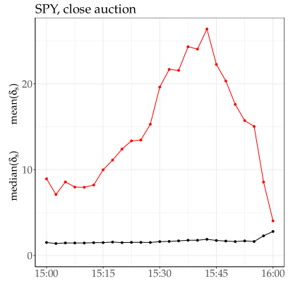
Figure 12: Mean and median distance between the indicative price and the mid price in units of spreads $\delta_{s}=|\pi-m|/s$ as a function time for SPY when the indicative price is outside of the spread; left plot: open auction, right plot: close auction)

We first report the fraction of time (in units of updates) spent by the indicative price in the spread, i.e., $P[b(t)\leq\pi(t)\leq a(t)]$ for an update chosen at random in a given a time slice. Figure 11 reports the average spread (in bps) $\tilde{s}=(a-b)/m$ versus the average $P[b(t)\leq\pi(t)\leq a(t)]$ for all assets (average here means average over the time-slice averages, themselves averaged over days for a given asset). For open auctions, one finds that $\tilde{s}\propto\exp P[b(t)\leq\pi(t)\leq a(t)]$. In other words, defining the relative deviation of the indicative price by $\delta_{m}=|\pi-m|/m$ and assuming that the distribution of $\delta_{m}$ is the same for all these assets and independent from $\tilde{s}$, we find

$$P[b(t)\leq\pi(t)\leq a(t)]=P(\delta_{m}\leq\tilde{s}/2)\propto\log\tilde{s},$$

hence $P(\delta_{m})\propto 1/\delta_{m}$: this simple (and rough) argument indicates that the distribution of relative distance of the indicative price and the mid price, aggregated over all the assets, is heavy-tailed and that the indicative price cares little about being in the spread; this is due in part to the fact that the gaps between occupied ticks in the auction book are very likely heavy tailed, given the fact that regular trading hours limit order books are sparse provided that the relative tick size is not too large (Gillemot et al., 2006). We checked that there is no universal $P_{>}(\delta_{m})$ for all the assets, but that it is generally heavy-tailed (see e.g. $P_{>}(\delta_{m})\simeq 1/\delta_{m}$ for SPY in Fig. 11). Close auctions take place during regular trading hours, i.e., when the typical spread is much smaller. If the indicative price has no special reason to be within the spread, thus is not bound by a strong force to the spread, one expects that the fraction of time it spends in the spread is smaller than during the open auction. This is exactly what happens (see Fig. 11). When the indicative price is outside of the spread, it is typically less than 2 spreads away (Fig. 12), whereas its average may be much larger at times, especially when the spread is small. Interestingly, the typical mean deviation displays the same behaviour for the open and close auctions: a steady increase followed by a steeper decrease, with an additional peak at 8:30, a time at which, as remarked above, a sizeable fraction of volume is sent for this particular asset (SPY).

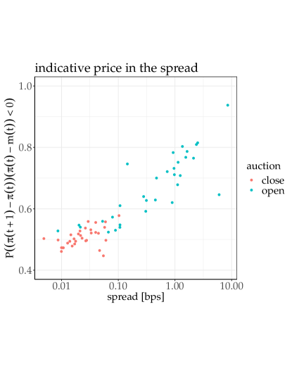
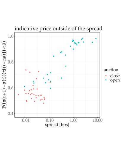
Figure 13: Probability of indicative price reversion towards the mid price as a function of the average spread when the indicative price is in the spread (left plot) and outside of the spread (right plot)

A robust way to measure how the indicative price is attracted by the mid price is the probability that an indicative price change brings it closer to the mid price, in other words the reversion probability $P[(\pi(t+1)-\pi(t))(\pi(t)-m(t))<0]$. Figure 13 plots the reversion probability as a function of the spread; the larger the average spread, the larger the reversion probability when $\pi$ is in the spread, for both auctions. When $\pi$ is outside of the spread, the reversion does not depend on the average spread for close auctions, but clearly does for open auctions. To check how frequent overshooting is, we also measured $P[(\pi(t+1)-m(t+1))(\pi(t)-m(t))<0|\pi\textrm{ not in spread}]$, whose average over the assets is about 0.02 for open auctions, and 0.05 for close auctions, i.e., quite small.

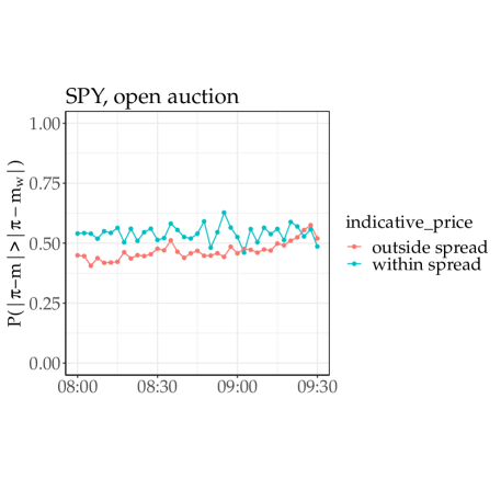
Figure 14: Probability that the indicative price is closer to the weighted mid price $m_{w}$ than the mid price $m$ as function of time both the open auction (left plot) and the close auction (right plot).

Finally, we checked if the indicative price was closer to the mid or to the weighted mid price by estimating the fraction of times $|\pi(t)-m(t)|>|\pi(t)-m_{w}(t)|$ when the indicative price is in the spread and outside of it. The difference is small but real (see Fig. 14). The average $P(|\pi(t)-m(t)|>|\pi(t)-m_{w}(t)|)\simeq 0.45$ over all time slices and the 35 most liquid assets. In other words, the mid price is a slightly more trustworthy reference point than the weighted mid price. Whether the indicative price is in or outside of the spread has no influence on the estimate.

5 Conclusions

The dynamical properties of the auction processes are far from trivial and markedly different from those of the open-market limit order books. First, because the imbalance process is mean-reverting, indicative prices are under-diffusive. Second, the median response functions at the opening and closing auctions may have opposite signs. Three important ingredients are responsible for these differences. First, auctions at fixed times force the traders to reveal all liquidity before the auction, thus increasing the importance of strategic order submission timing, as shown at times by the large relative cancellation of liquidity just before the auction ending time, or the acceleration of the fraction of matched volume a few minutes before the auction ending time for some assets. Second, during the auction process, no trade originates from the auction book building-up; as a consequence, usual price efficiency conditions do not apply here. Quite notably in the US exchanges studied here, continuous double auctions run in parallel to the auction processes; this is one of the reasons why the opening auction response functions are very different from those of the closing auctions: indeed, during the closing auction, the relative liquidity available on the open-market limit order book is much larger than that of outside regular trading hours during the opening auction. Finally, the indicative price may be rather far from the mid price of the regular limit order book, although on average, the former reverts to the latter with non-negligible probability.

Because data availability, our results on pre-auction periods are mostly about NYSE Arca, i.e., mostly about ETFs. Future work will use better data in order to check if the above findings also hold for more usual equities. Given the mechanisms discussed above, this is not unlikely.

N. G. thanks CentraleSupélec for an extended stay during which part of this work was carried out. We thank Fabrizio Lillo and Thierry Bochud for stimulating discussions. We also thank Cédric Joulain for providing us with his LispTick fast data streaming framework. The source code used for data analysis is freely available at https://github.com/damienchallet.

References

- (1)
- Alfi et al. (2009) Alfi, V., Gabrielli, A., Pietronero, L., 2009, How People React to a Deadline: Time Distribution of Conference Registrations and Fee Payments. Open Physics 7, 483–489.
- Alfi et al. (2007) Alfi, V., Parisi, G., Pietronero, L., 2007, Conference Registration: How People React to a Deadline. Nature Physics 3, 746–746.
- Alstott et al. (2014) Alstott, J., Bullmore, E., Plenz, D., 2014, powerlaw: a Python Package for Analysis of Heavy-tailed Distributions. PloS one 9, p. e85777.
- Bellia et al. (2016) Bellia, M., Pelizzon, L., Subrahmanyam, M. G., Uno, J., Yuferova, D., 2016, Low-latency Trading and Price Discovery: Evidence from the Tokyo Stock Exchange in the Pre-opening and Opening Periods.
- Borle et al. (2006) Borle, S., Boatwright, P., Kadane, J. B., 2006, The Timing of Bid Placement and Extent of Multiple Bidding: An Empirical Investigation Using eBay Online Auctions. Statistical Science, 194–205.
- Bouchaud et al. (2006) Bouchaud, J. P., Kockelkoren, J., Potters, M., 2006, Random Walks, Liquidity Molasses and Critical Response in Financial Markets. Quantitative Finance 6, 115–123.
- Boussetta et al. (2016) Boussetta, S., Lescourret, L., Moinas, S., 2016, The Role of Pre-Opening Mechanisms in Fragmented Markets.
- Challet (2019) Challet, D. 2019, Strategic behaviour and indicative price diffusion in Paris Stock Exchange auctions. In proceedings of Dehli Econophys APEC 2017.
- Chelley-Steeley (2008) Chelley-Steeley, P. L., 2008, Market Quality Changes in the London Stock Market. Journal of Banking & Finance 32, 2248–2253.
- Clauset et al. (2009) Clauset, A., Shalizi, C. R., Newman, M. E., 2009, Power-law distributions in empirical data. SIAM review 51, 661–703.
- Gillemot et al. (2006) Gillemot, L., Farmer, J. D., Lillo, F., 2006, There’s more to volatility than volume. Quantitative Finance 6, 371–384.
- Gu et al. (2008) Gu, G.-F., Chen, W., Zhou, W.-X., 2008, Empirical Regularities of Order Placement in the Chinese Stock Market. Physica A: Statistical Mechanics and its Applications 387, 3173–3182.
- Gu et al. (2010) Gu, G.-F., Ren, F., Ni, X.-H., Chen, W., Zhou, W.-X., 2010, Empirical Regularities of Opening Call Auction in Chinese Stock Market. Physica A: Statistical Mechanics and its Applications 389, 278–286.
- Kissell and Lie (2011) Kissell, R., Lie, H., 2011, US Exchange Auction Trends: Recent Opening and Closing Auction Behavior, and the Implications on Order Management Strategies. The Journal of Trading 6, 10–30.
- Lehalle and Laruelle (2018) Lehalle, C.-A., Laruelle, S. 2018, Market microstructure in practice., World Scientific, 2nd edition.
- Pagano et al. (2013) Pagano, M. S., Peng, L., Schwartz, R. A., 2013, A Call Auction’s Impact on Price Formation and Erder Routing: Evidence from the NASDAQ Stock Market. Journal of Financial Markets 16, 331–361.
- Pagano and Schwartz (2003) Pagano, M. S., Schwartz, R. A., 2003, A Closing Call’s Impact on Market Quality at Euronext Paris. Journal of Financial Economics 68, 439–484.
- Toth et al. (2012) Toth, B., Eisler, Z., Lillo, F., Kockelkoren, J., Bouchaud, J.-P., Farmer, J. D., 2012, How does the market react to your order flow? Quantitative Finance 12, 1015–1024.
- Vuong (1989) Vuong, Q. H., 1989, Likelihood Ratio Tests for Model Selection and Non-nested Hypotheses. Econometrica: Journal of the Econometric Society, 307–333.