Theory of optical forces on small particles by multiple plane waves

Abstract

We theoretically investigate the optical force exerted on an isotropic particle illuminated by a superposition of plane waves. We derive explicit analytical expressions for the exerted force up to quadrupolar polarizabilities. Based on these analytical expressions, we demonstrate that an illumination consisting of two tilted plane waves can provide a full control on the optical force. In particular, optical pulling, pushing and lateral forces can be obtained by the proper tuning of illumination parameters. Our findings might unlock multiple applications based on a deterministic control of the spatial motion of small particles.

I Introduction

Light as an electromagnetic radiation carries energy and momentum. The direction of energy flux of an electromagnetic wave at any point in space-time is given by the Poynting vector $\mathbf{S}(\mathbf{r},t)$ and the linear momentum density (i.e. linear momentum per unit volume) is given by $\mathbf{S}(\mathbf{r},t)/c^{2}$, where $c$ is the speed of light Zangwill (2013). The exchange of linear momentum of light with an electromagnetically interacting particle can lead to an exerted optical force, known as the radiation pressure. In general, the acceleration caused by the radiation pressure on heavy macroscopic objects is considerably small. However, this acceleraion can be considerably large for small particles (compared to wavelength) when illuminated by a light beam with a moderate intensity. Therefore, light beams can be used to move, trap, or guide a particle. This became experimentally feasible after the invention of lasers and the challenge was overcome by Arthur Ashkin that used a single weakly focused laser beam/two counter-propagating beams to move/trap microparticles Ashkin et al. (1987); Ashkin (1970). From then on, the technique has been widely used to manipulate atoms, molecules Raab et al. (1987); Ashkin (1978), and biological cells Welte et al. (1998); Ashkin et al. (1987); and it has opened a brand new field of research termed as optical manipulation Grier (2003); Maragò et al. (2013).

Besides, one can have further control on the direction of the exerted optical force and achieve counter-intuitive forces like the optical pulling or lateral forces Chen et al. (2011); Sáenz (2011); Novitsky et al. (2011); Dogariu et al. (2013); Brzobohatỳ et al. (2013); Rodríguez-Fortuño et al. (2015); Alaee et al. (2018a). The former being also called an optical tractor beam. These forces have been obtained by engineering the excitation and particle’s symmetry and material. In particular, optical pulling force on an isotropic particle can be obtained through the interference of multiple plane waves, solenoidal beams Grier et al. (2014), or Bessel beams Chen et al. (2015). Furthermore, employing chiral particles, gain media, or plasmonic interfaces can also allow achieving exerted lateral and pulling forces on the particle Webb et al. (2011); Ding et al. (2014); Novitsky and Qiu (2014); Wang and Chan (2014); Canaguier-Durand and Genet (2015); Fernandes and Silveirinha (2015, 2016); Liu et al. (2017); Petrov et al. (2016); Alaee et al. (2018a).

Multipole expansion is a key tool to study several optical phenomena namely, light perfect absorption Landy et al. (2008); Alaee et al. (2016, 2017), directional light emission Person et al. (2013); Hancu et al. (2013); Fu et al. (2013); Coenen et al. (2014); Alaee et al. (2015), manipulating and controlling spontaneous emission Rogobete et al. (2007); Zambrana-Puyalto and Bonod (2015); Doeleman et al. (2016), electromagnetically-induced-transparency Chiam et al. (2009), Fano resonances Luk’yanchuk et al. (2010); Miroshnichenko et al. (2010), electromagnetic cloaking Alù and Engheta (2008, 2009), and also optical force Chaumet and Nieto-Vesperinas (2000); Hayat et al. (2015); Guclu et al. (2015); Mobini et al. (2017); Albooyeh et al. (2017); Kamandi et al. (2017) and torque Bishop et al. (2003); Nieto-Vesperinas (2015); Chang and Lee (1985); Rahimzadegan et al. (2016) among many others. For small particles compared to the wavelength, induced electric and magnetic dipole and quadrupole moments are usually sufficient to fully understand the underlying physics. In this paper, we derive analytical expressions for the exerted optical force based on multipole expansion Bohren and Huffman (2008); Xu (1995); Barton et al. (1989); Almaas and Brevik (1995); Rahimzadegan et al. (2017) up to quadrupolar polarizabilities. Detailed derivations are given in the supplementary material. We theoretically and numerically study optical pulling, pushing, and lateral forces exerted on an isotropic particle for single and two tilted plane waves. The conditions for optical pushing, pulling, and lateral forces are discussed. In particular, we explore the effects of the illumination parameters i.e the wavelength, the angle between the two plane waves, and the position of the particle on the exerted optical force. The analytical expressions (Theory) are verified with the numerical solution of Maxwell’s equations using COMSOL (Simulation). The electric and magnetic fields obtained through the simulations are employed to calculate the Maxwell stress tensor and finally the optical force can be calculated accordingly, see Eq. (1). In the following, we focus on the underlying theory and explain our results and its physical implications.

II Theory

The time averaged mechanical force exerted on an arbitrary particle by an optical wave can be calculated as Jackson (1999); Novotny and Hecht (2012); Zangwill (2013):

$$\left\langle\mathbf{F}\right\rangle=\left\langle\underset{s}{\oint}{\underline{\mathbf{T}}}(\mathbf{r},t)\cdot\mathbf{n}\mathrm{d}S\right\rangle,$$ (1)

with $S$ being any closed surface surrounding the particle, $\mathbf{n}$ the outward unit normal vector to the surface, and ${\underline{\mathbf{T}}}$ the Maxwell’s stress tensor. The underline denotes the time-domain expressions. The Maxwell stress tensor (MST) is a tensor of second rank whose elements are defined as Jackson (1999); Novotny and Hecht (2012):

$$\underline{T}_{ij}=\varepsilon_{0}\left[\underline{E}_{i}\underline{E}_{j}+c^{2}\underline{B}_{i}\underline{B}_{j}-\frac{1}{2}\delta_{ij}\left(|\underline{\mathbf{E}}|^{2}+|\underline{\mathbf{B}}|^{2}\right)\right]$$ (2)

where $\underline{E}$, $\underline{B}$ are the total (incoming plus scattered) electric and magnetic fields in the $i,j=x,y,z$ axis, respectively. $\delta_{ij}$ represents the Kronecker delta function.

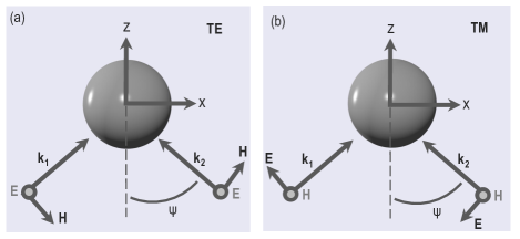
Figure 1: (a)-(b) The schematic of an isotropic particle illuminated by two tilted linearly polarized transverse electric (TE) and transverse magnetic (TM) plane waves, respectively.

Although the method based on the MST provides the exact solution, it does not suit the interpretative understanding of the light-matter interaction. To this end, we use the multipole expansion method. We decompose the induced current density in the particle in terms of the electric and the magnetic multipole moments. For a small polarizable particle (compared to wavelength), depending on the geometry, material, and the illumination, the decomposition of induced current leads to the definition of the electric and magnetic dipole and quadrupole polarizabilities (neglecting the higher order polarizabilities). The induced electric and magnetic dipoles in Cartesian coordinates for an isotropic particle are expressed in terms of electric ($\alpha^{e}$) and magnetic ($\alpha^{m}$) polarizabilities as $\mathbf{p}=\varepsilon_{0}\alpha^{e}\mathbf{E}$ and $\mathbf{m}=\alpha^{m}\mathbf{H}$, respectively. The electric and magnetic quadrupole moments for an isotropic particle is defined as Alù and Engheta (2009); Bernal Arango et al. (2014):

$$\mathbf{Q}^{e} = \varepsilon_{0}\alpha_{Q^{e}}\frac{\nabla\mathbf{E}+\mathbf{E}\nabla}{2},$$

$$\mathbf{Q}^{m} = \alpha_{Q^{m}}\frac{\nabla\mathbf{H}+\mathbf{H}\nabla}{2},$$

where $\alpha_{Q^{e}}$ and $\alpha_{Q^{m}}$ are the Cartesian quadrupolar polarizabilities. Using the relation $\left(\nabla\mathbf{A}+\mathbf{A}\nabla\right)_{ij}=\partial_{i}A_{j}+\partial_{j}A_{i}$, any component of $Q^{e}$ and $Q^{m}$ is calculated as $Q_{ij}^{e}=\varepsilon_{0}\alpha_{Q^{e}}\left(\partial_{i}E_{j}+\partial_{j}E_{i}\right)/2$ and $Q_{ij}^{m}=\alpha_{Q^{m}}\left(\partial_{i}H_{j}+\partial_{j}H_{i}\right)/2$, respectively.

The optical force exerted on a particle by an arbitrary illumination can be written as the following (truncated at quadrupole order) Barton et al. (1989); Almaas and Brevik (1995); Rahimzadegan et al. (2017):

$$\mathbf{F} = \left[\mathbf{F}_{p}+\mathbf{F}_{Q^{e}}+...\right]+\left[\mathbf{F}_{m}+\mathbf{F}_{Q^{m}}+...\right]$$

$$+\left[\mathbf{F}_{pm}+\mathbf{F}_{Q^{e}Q^{m}}+...\right]$$

$$+ \left[\mathbf{F}_{pQ^{e}}+...\right]+\left[\mathbf{F}_{mQ^{m}}+...\right],$$

where $\mathbf{F}_{p}(\mathbf{F}_{m})$ is the individual contribution of an electric (magnetic) dipole moment to the total optical force. $\mathbf{F}_{Q^{e}}(\mathbf{F}_{Q^{m}})$ is the contribution of an individual electric (magnetic) quadrupole moment; and the other expressions are the contribution of the interference between two multipole moments.

Neglecting higher order terms, Eq. (II) can be rewritten in terms of Cartesian dipole and quadrupole moments as follows Barton et al. (1989); Almaas and Brevik (1995); Chen et al. (2011); Rahimzadegan et al. (2017):

$$F_{i} = \frac{1}{2}\textrm{Re}\left[\underset{j}{\sum}p_{j}\nabla_{i}E_{j}^{*}\right]+\frac{1}{2}\textrm{Re}\left[\underset{j}{\sum}m_{j}\nabla_{i}B_{j}^{*}\right]-\frac{k^{4}}{12\pi\varepsilon_{0}c}\textrm{Re}\left[\underset{j,k}{\sum}\epsilon_{ijk}p_{j}m_{k}^{*}\right]$$ (4)

$$- \frac{k^{5}}{120\pi\varepsilon_{0}}\textrm{Im}\left[\underset{j}{\sum}\left(Q^{e}\right)_{ij}p_{j}^{*}\right]+\frac{1}{\text{12}}\textrm{Re}\left[\left(Q^{e}\right)_{jk}\nabla_{i}\nabla_{k}E_{j}^{*}\right]+\frac{k^{5}}{120\pi\varepsilon_{0}c^{2}}\textrm{Im}\left[\left(Q^{m}\right)_{ij}m_{j}^{*}\right]$$

$$+ \frac{1}{12}\mathrm{Re}\left[\underset{k}{\sum}\left(Q^{m}\right)_{jk}\nabla_{i}\nabla_{k}B_{j}^{*}\right]-\frac{k^{6}}{9\times 240\pi\varepsilon_{0}c}\mathrm{Re}\left[\underset{l,j,k}{\sum}\varepsilon_{ijk}(Q^{e})_{lj}\left(Q^{m}\right)_{lk}^{*}\right],$$

in which $E_{i}$ and $B_{i}$ are components of the incident electric and magnetic fields, respectively, and $\epsilon_{ijk}$ is the Levi-Civita symbol.

As shown in Fig. 1, consider an illumination composed of two tilted plane waves with wave vectors $\mathrm{\mathbf{k}}_{1}=k[\mathrm{sin\psi},0,\mathrm{cos\psi}]$ and $\mathrm{\mathbf{k}}_{2}=k[-\mathrm{sin\psi},0,\mathrm{cos\psi}]$, illuminating an isotropic particle, where $\psi$ is the tilting angle. We define the TE and TM illuminations as the following:

$$\mathbf{E^{\mathrm{TE}}} = \frac{E_{0}}{2}\left(e^{i\mathbf{k}_{1}\cdot\mathbf{r}}+e^{i\mathbf{k}_{2}\cdot\mathbf{r}}\right)\mathbf{e}_{y},$$ (5)

$$\mathrm{\mathbf{E}}^{\mathrm{TM}} = \frac{E_{0}}{2}\left(\left[\begin{array}[]{c}\mathrm{cos}\psi\\ 0\\ -\mathrm{sin}\psi\end{array}\right]e^{i\mathbf{k}_{1}\cdot\mathbf{r}}+\left[\begin{array}[]{c}\mathrm{cos}\psi\\ 0\\ \mathrm{sin}\psi\end{array}\right]e^{i\mathbf{k}_{2}\cdot\mathbf{r}}\right).$$ (12)

The time averaged optical forces exerted on an isotropic particle located at the position $\mathbf{r}_{0}=\left(x_{0},y_{0},z_{0}\right)$ by the TE and TM illuminations, i.e. Eqs. (5)-(12) read as (see supplementary material):

$$\mathbf{\overline{F}}^{\mathrm{TE}} \approx \mathbf{\overline{F}}_{p}^{\mathrm{TE}}+\mathbf{\overline{F}}_{m}^{\mathrm{TE}}+\overline{\mathbf{F}}_{pm}^{\mathrm{TE}}+\mathbf{\overline{F}}_{Q^{e}}^{\mathrm{TE}}+\mathbf{\overline{F}}_{Q^{m}}^{\mathrm{TE}}+\mathbf{\overline{F}}_{pQ^{e}}^{\mathrm{TE}}+\mathbf{\overline{F}}_{mQ^{m}}^{\mathrm{TE}}+\mathbf{\overline{F}}_{Q^{e}Q^{m}}^{\mathrm{TE}},$$ (13)

$$\overline{\mathbf{F}}_{p}^{\mathrm{TE}} = -\frac{3}{2}\mathrm{sin}\psi\mathrm{sin}2\delta\mathrm{Re}\left(\bar{\alpha_{e}}\right)\mathbf{e}_{x}+3\mathrm{cos}\psi\mathrm{cos^{2}}\delta\mathrm{Im}\left(\bar{\alpha_{e}}\right)\mathbf{e}_{z},$$

$$\overline{\mathbf{F}}_{m}^{\mathrm{TE}} = -\frac{3}{2}\mathrm{sin}\psi\mathrm{sin}2\delta\mathrm{cos2\psi}\mathrm{Re}\left(\bar{\alpha}_{m}\right)\mathbf{e}_{x}+3\mathrm{cos}\psi\left(\mathrm{cos^{2}\psi cos^{2}}\delta+\mathrm{sin^{2}}\psi\mathrm{sin^{2}}\delta\right)\mathrm{Im}\left(\bar{\alpha_{m}}\right)\mathbf{e}_{z},$$

$$\overline{\mathbf{F}}_{pm}^{\mathrm{TE}} = -\frac{3}{2}\mathrm{sin\psi}\mathrm{sin}2\delta\mathrm{Im}\left(\bar{\alpha_{e}}\bar{\alpha}_{m}^{*}\right)\mathbf{e}_{x}-3\mathrm{cos}\psi\mathrm{cos^{2}}\delta\mathrm{Re}\left(\bar{\alpha_{e}}\bar{\alpha}_{m}^{*}\right)\mathbf{e}_{z},$$

$$\overline{\mathbf{F}}_{Q^{e}}^{\mathrm{TE}} = -\frac{5}{2}\mathrm{sin}\psi\mathrm{sin}2\delta\mathrm{cos}2\psi\mathrm{Re}\left(\bar{\alpha}_{Q^{e}}\right)\mathbf{e}_{x}+5\mathrm{cos}\psi\left(\mathrm{cos^{2}\psi cos^{2}}\delta+\mathrm{sin^{2}}\psi\mathrm{sin^{2}}\delta\right)\mathrm{Im}\left(\bar{\alpha}_{Q^{e}}\right)\mathbf{e}_{z},$$

$$\overline{\mathbf{F}}_{Q^{m}}^{\mathrm{TE}} = -\frac{5}{2}\mathrm{sin}\psi\mathrm{sin}2\delta\mathrm{cos4\psi}\mathrm{Re}\left(\bar{\alpha}_{Q^{m}}\right)\mathbf{e}_{x}+5\mathrm{cos}\psi\left(\mathrm{cos^{2}2\psi cos^{2}}\delta+\mathrm{sin^{2}2\psi sin^{2}}\delta\right)\mathrm{Im}\left(\bar{\alpha}_{Q^{m}}\right)\mathbf{e}_{z},$$

$$\overline{\mathbf{F}}_{pQ^{e}}^{\mathrm{TE}} = +\frac{3}{2}\mathrm{sin}\psi\mathrm{sin}2\delta\mathrm{Im\left(\bar{\alpha}_{Q^{e}}\bar{\alpha}_{e}^{*}\right)}\mathbf{e}_{x}-3\mathrm{cos}\psi\mathrm{cos^{2}}\delta\mathrm{Re}\left(\bar{\alpha}_{Q^{e}}\bar{\alpha}_{e}^{*}\right)\mathbf{e}_{z},$$

$$\overline{\mathbf{F}}_{mQ^{m}}^{\mathrm{TE}} = +\frac{3}{2}\mathrm{sin}\psi\mathrm{sin}2\delta\left(\mathrm{cos2\psi+2cos^{2}\psi}\right)\mathrm{Im}\left(\bar{\alpha}_{Q^{m}}\bar{\alpha}_{m}^{*}\right)\mathbf{e}_{x}-3\mathrm{cos}\psi\left(\mathrm{cos}2\psi\mathrm{cos^{2}}\delta+2\mathrm{sin^{2}}\psi\mathrm{sin^{2}}\delta\right)\mathrm{Re}\left(\bar{\alpha}_{Q^{m}}\bar{\alpha}_{m}^{*}\right)\mathbf{e}_{z},$$

$$\overline{\mathbf{F}}_{Q^{e}Q^{m}}^{\mathrm{TE}} = -\frac{5}{6}\mathrm{sin\psi\mathrm{sin}2\delta\mathrm{\left(cos2\psi+2cos^{2}\psi\right)}Im}\left(\bar{\alpha}_{Q^{e}}\bar{\alpha}_{Q^{m}}^{*}\right)\mathbf{e}_{x}-\frac{5}{3}\mathrm{cos}\psi\left(\mathrm{cos}2\psi\mathrm{cos^{2}}\delta+2\mathrm{sin^{2}\psi sin^{2}}\delta\right)\mathrm{Re}\left(\bar{\alpha}_{Q^{e}}\bar{\alpha}_{Q^{m}}^{*}\right)\mathbf{e}_{z},$$

$$\overline{\mathbf{F}}^{\mathrm{TM}} \approx \mathbf{\overline{F}}_{p}^{\mathrm{TM}}+\mathbf{\overline{F}}_{m}^{\mathrm{TM}}+\mathbf{\overline{F}}_{pm}^{\mathrm{TM}}+\mathbf{\overline{F}}_{Q^{e}}^{\mathrm{TM}}+\mathbf{\overline{F}}_{Q^{m}}^{\mathrm{TM}}+\mathbf{\overline{F}}_{pQ^{e}}^{\mathrm{TM}}+\mathbf{\overline{F}}_{mQ^{m}}^{\mathrm{TM}}+\mathbf{\overline{F}}_{Q^{e}Q^{m}}^{\mathrm{TM}},$$ (14)

$$\mathbf{\overline{F}}_{p}^{\mathrm{TM}} = -\frac{3}{2}\mathrm{sin\psi}\mathrm{sin}2\delta\mathrm{cos2}\psi\mathrm{Re}\left(\bar{\alpha_{e}}\right)\mathbf{e}_{x}+3\mathrm{cos}\psi\mathrm{\left(\mathrm{cos^{2}\psi cos^{2}}\delta+\mathrm{sin^{2}}\psi\mathrm{sin^{2}}\delta\right)\mathrm{Im}\left(\bar{\alpha_{e}}\right)}\mathbf{e}_{z},$$

$$\mathbf{\overline{F}}_{m}^{\mathrm{TM}} = -\frac{3}{2}\mathrm{sin\psi}\mathrm{sin}2\delta\mathrm{Re}\left(\bar{\alpha_{m}}\right)\mathbf{e}_{x}+3\mathrm{cos}\psi\mathrm{cos^{2}}\delta\mathrm{Im}\left(\bar{\alpha_{m}}\right)\mathbf{e}_{z},$$

$$\mathbf{\overline{F}}_{pm}^{\mathrm{TM}} = +\frac{3}{2}\mathrm{sin\psi}\mathrm{sin}2\delta\mathrm{Im}\left(\bar{\alpha_{e}}\bar{\alpha}_{m}^{*}\right)\mathbf{e}_{x}-3\mathrm{cos}\psi\mathrm{cos^{2}}\delta\mathrm{Re}\left(\bar{\alpha_{e}}\bar{\alpha}_{m}^{*}\right)\mathbf{e}_{z},$$

$$\mathbf{\overline{F}}_{Q^{e}}^{\mathrm{TM}} = -\frac{5}{2}\mathrm{sin}\psi\mathrm{sin}2\delta\mathrm{cos}4\psi\mathrm{Re}\left(\bar{\alpha}_{Q^{e}}\right)\mathbf{e}_{x}+5\mathrm{cos}\psi\left(\mathrm{cos^{2}2\psi cos^{2}}\delta+\mathrm{sin^{2}2\psi sin^{2}}\delta\right)\mathrm{Im}\left(\bar{\alpha}_{Q^{e}}\right)\mathbf{e}_{z},$$

$$\mathbf{\overline{F}}_{Q^{m}}^{\mathrm{TM}} = -\frac{5}{2}\mathrm{sin}\psi\mathrm{sin}2\delta\mathrm{cos2\psi}\mathrm{Re}\left(\bar{\alpha}_{Q^{m}}\right)\mathbf{e}_{x}+5\mathrm{cos}\psi\left(\mathrm{cos^{2}\psi cos^{2}}\delta+\mathrm{sin^{2}}\psi\mathrm{sin^{2}}\delta\right)\mathrm{Im}\left(\bar{\alpha}_{Q^{m}}\right)\mathbf{e}_{z},$$

$$\mathbf{\overline{F}}_{pQ^{e}}^{\mathrm{TM}} = +\frac{3}{2}\mathrm{sin}\psi\mathrm{sin}2\delta\left(\mathrm{cos2\psi+2cos^{2}\psi}\right)\mathrm{Im}\left(\bar{\alpha}_{Q^{e}}\bar{\alpha}_{e}^{*}\right)\mathbf{e}_{x}-3\mathrm{cos}\psi\left(\mathrm{cos^{2}}\delta\mathrm{cos}2\psi+2\mathrm{sin^{2}}\psi\mathrm{sin^{2}}\delta\right)\mathrm{Re}\left(\bar{\alpha}_{Q^{e}}\bar{\alpha}_{e}^{*}\right)\mathbf{e}_{z},$$

$$\mathbf{\overline{F}}_{mQ^{m}}^{\mathrm{TM}} = +\frac{3}{2}\mathrm{sin}\psi\mathrm{sin}2\delta\mathrm{Im}\left(\bar{\alpha}_{Q^{m}}\bar{\alpha}_{m}^{*}\right)\mathbf{e}_{x}-3\mathrm{cos}\psi\mathrm{cos^{2}}\delta\mathrm{Re}\left(\bar{\alpha}_{Q^{m}}\bar{\alpha}_{m}^{*}\right)\mathbf{e}_{z},$$

$$\overline{\mathbf{F}}_{Q^{e}Q^{m}}^{\mathrm{TM}} = +\frac{5}{6}\mathrm{sin}\psi\mathrm{sin}2\delta\left(\mathrm{\mathrm{cos2\psi+2cos^{2}\psi}}\right)\mathrm{Im}(\bar{\alpha}_{Q^{e}}\bar{\alpha}_{Q^{m}}^{*})\mathbf{e}_{x}-\frac{5}{3}\mathrm{cos}\psi\left(\mathrm{cos^{2}}\delta\mathrm{cos}2\psi+2\mathrm{sin^{2}\psi sin^{2}}\delta\right)\mathrm{Re}\left(\bar{\alpha}_{Q^{e}}\bar{\alpha}_{Q^{m}}^{*}\right)\mathbf{e}_{z}.$$

where we define $\bar{\alpha}_{e,m}=\alpha_{e,m}/\alpha_{d}$, $\bar{\alpha}_{Q^{e,m}}=\alpha_{Q^{e,m}}/\alpha_{q}$, and $\delta=k\mathrm{sin\psi}x_{0}$. $\alpha_{q}=120\pi/k^{5}$ and $\alpha_{d}=6\pi/k^{3}$ are the polarizability normalizations for dipoles and quadrupoles, respectively. Please note that a lateral change in $x_{0}$, being the spatial position of the particle, has the equivalent effect on the force as a phase shift $\Delta\phi=-2kx_{0}\sin\psi$ in the two plane waves illuminating the particle. This makes sense as the spatial interference pattern that the two plane waves form only depends on the phase difference. The optical force exerted on the particle only depends on its position along the $x$-axis while it is independent on the position along the $z$- and $y$-axis (i.e. it depends on $\delta=k\mathrm{sin\psi}x_{0}$). Throughout the paper, optical forces are normalized to $\mathrm{F}^{\mathrm{norm}}=\left(I_{0}/c\right)\left[\lambda^{2}/\left(2\pi\right)\right]=I_{0}k\alpha_{d}/\left(3c\right)$. The normalization factor of $\mathrm{F}^{\mathrm{norm}}$ is of physical significance and $\mathrm{3F}^{\mathrm{norm}}$ corresponds to the upper bound for the exerted optical force on an isotropic electric/magnetic dipolar particle illuminated by a plane wave Rahimzadegan et al. (2017).

III Theoretical and numerical results

In the following, we consider a dielectric sphere made from a material with a permittivity of $\varepsilon=3.5^{2}$, and radius $a$. Figure 2 shows the calculated polarizabilities. They are calculated by using electric and magnetic Mie coefficients (i.e. $a_{1},a_{2}$ and $b_{1},b_{2}$) Mie (1908):

$$\alpha_{e}=i\frac{6\pi}{k^{3}}a_{1}=i\alpha_{d}a_{1}, \alpha_{m}=i\frac{6\pi}{k^{3}}b_{1}=i\alpha_{d}b_{1},$$ (15)

$$\alpha_{Q^{e}}=i\frac{120\pi\epsilon_{0}}{k^{5}}a_{2}=i\alpha_{q}a_{2}, \alpha_{Q^{m}}=i\frac{120\pi}{k^{5}}b_{2}=i\alpha_{q}b_{2}.$$

Alternatively, they can be extracted from exact multipole moments based on induced current Fernandez-Corbaton et al. (2015); Alaee et al. (2018b). We restrict ourselves to the wavelength region in where the lowest order polarizabilities have their lowest order resonances. Having the polarizabilities, through Eqs. (13) and (14), the exerted optical force due to the contribution of different multipole moments can be derived. Below, we consider several scenarios for the illumination.

III.1 Single plane wave illumination

Assuming a plane wave excitation, i.e. $\psi=0$, using Eqs.(13) or (14) the normalized optical force exerted on an isotropic particle is calculated as:

$$\overline{\mathbf{F}} \approx 3\mathrm{Im}\left(\bar{\alpha}_{e}+\bar{\alpha}_{m}\right)+5\mathrm{Im}\left(\bar{\alpha}_{Q^{e}}+\bar{\alpha}_{Q^{m}}\right)$$

$$- 3\mathrm{Re}\left(\bar{\alpha}_{e}\bar{\alpha}_{m}^{*}+\bar{\alpha}_{Q^{e}}\bar{\alpha}_{e}^{*}+\bar{\alpha}_{Q^{m}}\bar{\alpha}_{m}^{*}+\frac{5}{9}\bar{\alpha}_{Q^{e}}\bar{\alpha}_{Q^{m}}^{*}\right)\mathbf{e}_{z}.$$

The theoretical results based on the derived equation are shown in Fig. 3. As a verification, the results of the COMSOL simulation are also shown in Fig. 3(c).

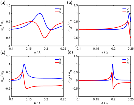
Figure 2: (a)-(b) Real and imaginary parts of the normalized Cartesian dipole and quadrupole polarizabilities of a sphere with permittivity $\varepsilon=3.5^{2}$ and radius $a$.

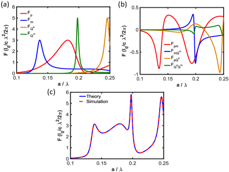
Figure 3: Single plane wave illumination: (a)-(b) Contribution of different moments to the multipolar force exerted by a single plane wave. (c) The exerted analytical and simulated optical force calculated by the analytical expression, i.e. Eq. (III.1) and the numerical approach based on MST, i.e. Eq. (1), respectively.

As can be seen in Fig. 3(a) and (b), interference terms can have negative (pulling) contributions to the total optical force, while the individual contributions of the moments are positive across the entire spectrum (the imaginary part of the polarizabilities is always positive for passive particles). With a single plane wave illumination, the total optical force is always positive (pushing), Fig. 3(c). Further, it can be observed that the quadrupolar terms have the dominant contributions to the highest values of the optical force at lower wavelengths. The optical force, as can be intuitively expected, is in the direction of the overall linear momentum, i.e. here, in the $z$-direction.

III.2 Two plane wave illumination: sphere at $\mathbf{r}=\mathbf{0}$

Assuming the sphere to be located in the center of the coordinate system, i.e $\mathbf{r}=(0,0,0)$, and being illuminated with the wave expressed by Eqs. 5-12, the calculated optical force as a function of the tilting angle $\psi$ and the particle’s size parameter, i.e. $a/\lambda$, is shown in Fig. 4(a) and (b) for TE- and TM-polarization, respectively. An optical pulling force is achieved for certain tilting angles for both TE and TM illuminations. This can be expected already by inspecting Eqs. (13)-(14), since the contribution of negative terms can dominate for some large angles as the positive terms are attenuating faster as the angle increases.
To make a better analysis of the negative force, we choose a smaller sized sphere, where dipole moments are dominant, and neglect the quadrupolar moments. Therefore, the optical force simplifies to:

$$\overline{\mathbf{F}} \approx \overline{\mathbf{F}}_{p}+\overline{\mathbf{F}}_{m}+\overline{\mathbf{F}}_{pm},$$ (17)

$$\mathrm{\overline{\mathbf{F}}^{TE}} \approx 3\mathrm{cos}\psi\left[\mathrm{Im}\left(\bar{\alpha}_{e}\right)+\mathrm{Im}\left(\bar{\alpha}_{m}\right)\mathrm{cos^{2}}\psi-\mathrm{Re}\left(\bar{\alpha}_{e}\bar{\alpha}_{m}^{*}\right)\right]\mathbf{e}_{z},$$

$$\mathrm{\overline{\mathbf{F}}^{TM}} \approx 3\mathrm{cos}\psi\left[\mathrm{Im}\left(\bar{\alpha}_{e}\right)\mathrm{cos^{2}}\psi+\mathrm{Im}\left(\bar{\alpha}_{m}\right)-\mathrm{Re}\left(\bar{\alpha}_{e}\bar{\alpha}_{m}^{*}\right)\right]\mathbf{e}_{z}.$$

The calculated optical force is shown in Fig. 5 for certain values of $a/\lambda=\left(1/7.52\right)$, $\left(1/5.26\right)$ for TE and TM illuminations, respectively.

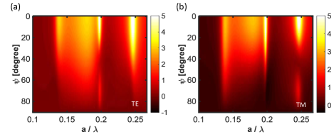
Figure 4: Two plane wave illumination and the sphere located at $\mathbf{r}=0$: (a)-(b) Exerted optical forces by two tilted plane waves as a function of the tilting angle and the particle’s size parameter, i.e. $a/\lambda$ for TE and TM illuminations, respectively.

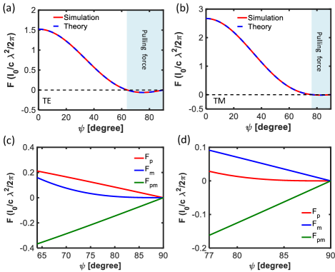
Figure 5: Two plane wave illumination and the sphere located at $\mathbf{r}=0$: (a)-(b) Exerted optical forces on the dielectric sphere, with permittivity $\varepsilon=3.5^{2}$, by two tilted plane waves at $a/\lambda=\left(1/7.52\right)$ and $\left(1/5.26\right)$ for TE and TM illuminations, respectively. (c)-(d) Contribution of different orders of dipoles and their interference to the optical force.

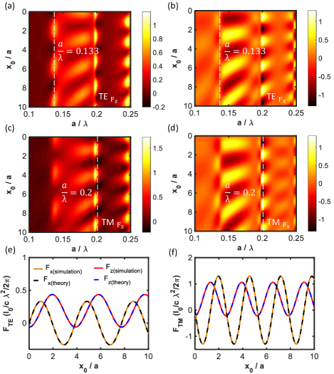
Figure 6: Two plane wave illumination and the sphere located at $\mathbf{r}=\mathbf{r}_{0}$: (a-d) Exerted optical forces on the dielectric sphere as a function of its position on the $x$-axis and its size parameter, i.e. $a/\lambda$ for TE and TM illuminations. (e,f) Periodic optical pushing/pulling forces on the dielectric sphere at $a/\lambda=0.133$ and $0.2$ for both TE and TM illuminations, respectively.

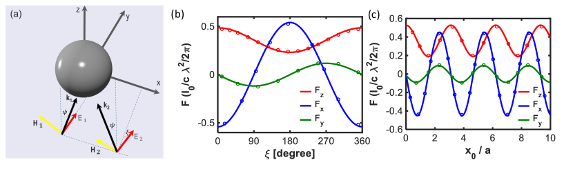
Figure 7: Two plane wave illumination using Eq. (24) and sphere located at $\mathbf{r}=\mathbf{r}_{0}$: (a) The schematic of an isotropic particle illuminated by two tilted linearly polarized plane waves. (b)-(c) Optical forces versus $\xi$ and $x_{0}/a$ exerted on the dielectric sphere with permittivity $\varepsilon=3.5^{2}$ and illuminated by two tilted linearly polarized plane waves at wavelength $\lambda=6\,a$ with angles ($\psi=75^{\circ}$, $x_{0}=a/2$). (c) for $\psi=75^{\circ},$ $\xi=45^{\circ}$. The solid line is the simulation and the circles are the analytical results calculated by using Eq. (25).

Based on this figure, for small values of the tilting angle $\psi$, a pushing force is exerted on the particle. As the tilting angle increases, for the TE(TM) polarization the magnitude of the force reduces until it vanishes at $\psi=62^{{\circ}}\left(76^{{\circ}}\right)$ and beyond that the pulling force appears, showing a minimum at $\psi=75^{\circ}\left(83^{{\circ}}\right)$. For both TE and TM illuminations, the terms $F_{p}$ and $F_{m}$ are positive, however, the term $F_{pm}$ in both cases is negative, canceling out the contributions of the positive terms at certain angles. Then, it becomes possible to reduce the positive contributions to the optical force and to achieve an overall negative force. In other words, according to Eq. (17) for TE (TM) polarization, the term $\overline{\mathbf{F}}_{m}$ ($\overline{\mathbf{F}}_{p}$) vanishes due to the term $\mathrm{cos^{3}}\psi$ for large $\psi$  [see Fig. 5 (a)-(d)]. Meanwhile, the overall force is decreased due to the term $\mathrm{cos}\psi$, a factor which appears as a total pre-factor.

III.3 Two plane wave illumination: sphere at $\mathbf{r}=\mathbf{r}_{0}$

In order to investigate the effects of the particle position $\mathbf{r}_{0}$ on the force exerted on it, which shows itself in the equations through the angle $\delta=k\mathrm{sin\psi}x_{0}$, the exerted optical forces as a function of the position and the particle’s size parameter, i.e. $a/\lambda$ is shown in Fig. 6 (a)-(d). The tilting angles for the TE and TM polarizations are $76^{\circ}$ and $73^{{\circ}}$, respectively. It can be seen that the particle experiences a periodic optical force. The existence of the lateral force is due to the gradient of the field intensity along the $x$-axis. Moreover, according to these figures it can be realized that the quadrupolar terms (around $a/\lambda=0.2$ and $0.25$, see also Figure 2) cause major variations of the optical force in amplitude and sign for both TE and TM illuminations. Figure 6 (e)-(f) depict the theoretical and simulated exerted forces (i.e. both $x$ and $z$ components) calculated for $a/\lambda=0.133$ and $0.2$ with the periodicity of $\Lambda=\lambda/\mathrm{sin}\psi$ with respect to the x-axis (see the definition of $\delta$). Theoretical results using Eq. (14) are in perfect agreement with the simulation results.

In order to explore other possible influences of two-plane wave illumination in the $x$-$z$-plane on the exerted optical force, the following generalized excitation is defined:

$$\mathrm{\mathbf{E}} = \frac{E_{0}}{2}\left(\left[\begin{array}[]{c}0\\ 1\\ 0\end{array}\right]e^{i\mathbf{k}_{1}\cdot\mathbf{r}}+\left[\begin{array}[]{c}\mathrm{cos}\psi\mathrm{sin}\xi\\ \mathrm{cos}\xi\\ \mathrm{sin}\psi\mathrm{sin}\xi\end{array}\right]e^{i\mathbf{k}_{2}\cdot\mathbf{r}}\right),$$ (24)

where $\xi$ is the deviation angle between electric field polarization of the two plane waves. The time averaged optical force exerted on an isotropic dipolar particle by the above illumination can be derived as:

$$\overline{\mathrm{F}}_{x} = -\frac{3}{2}\left[\mathrm{Re}\left(\bar{\alpha}_{e}\right)+\mathrm{Re}\left(\bar{\alpha}_{m}\right)\mathrm{cos}2\psi-\mathrm{Re}\left(\bar{\alpha}_{e}\bar{\alpha}_{m}^{*}\right)\right]$$

$$\mathrm{sin}\psi\mathrm{cos}\xi\mathrm{sin}2\delta,$$

$$\overline{\mathrm{F}}_{y} = \frac{3}{2}\left[\mathrm{Re}\left(e^{-2i\delta}\bar{\alpha}_{e}\bar{\alpha}_{m}^{*}\right)\right]\mathrm{sin}\psi\mathrm{sin}\xi\mathrm{cos}\psi,$$

$$\overline{\mathrm{F}}_{z} = \frac{3}{2}\mathrm{cos}\psi\left\{\left(1+\mathrm{cos}2\psi\mathrm{cos}\xi\mathrm{cos}2\delta\right)\mathrm{Im}(\bar{\alpha}_{m})\right.$$ (25)

$$\left.+\left[\mathrm{Im}(\bar{\alpha}_{e})-\mathrm{Re}(\bar{\alpha}_{e}\bar{\alpha}_{m}^{*})\right]\left(1+\mathrm{cos}\xi\mathrm{cos}2\delta\right)\right\}.$$

Intuitively, one might expect to have an exerted optical force only in the direction of the overall linear momentum, i.e. $\mathrm{\mathbf{k}}_{1}+\mathrm{\mathbf{k}}_{2}=2k\mathrm{cos}\psi\mathbf{e}_{z}$. However, according to Eq. (25), lateral forces (in both directions of $x$ and $y$) can be experienced by a fully symmetric (isotropic) particle for certain angles of $\psi$ and $\xi$. These peculiar lateral forces can be elaborated on the basis of the symmetry breaking mediated by the illuminating wave rather than the particle. The variation of lateral optical forces exerted on the dielectric sphere for parameters $\xi$, $\psi=75^{\circ}$, $x_{0}=a/2$ and $\psi=75^{\circ},$ $\xi=45^{\circ}$ are illustrated in Fig. 7 (a)-(b), respectively.

IV Conclusion

In conclusion, we investigated the optical force exerted on an isotropic particle by two plane waves and demonstrated theoretically that pushing-pulling forces for either TE or TM illuminations is possible. Our method, based on the theoretical calculations of multipolar forces, revealed the contribution of each electric and magnetic moment up to quadrupole terms (including their interferences) to the optical force. Additionally, this approach elaborates the optical force in a closed form due to the electrodynamical formalism of all influential parameters i.e. the designated angles, polarizabilities and amplitudes for either TE or TM illuminations. According to this formalism, we also showed the existence of lateral forces, in both $x$ and $y$ directions, for certain angles of $\psi$, $\xi$ and an interval of deviation of the object from the center $x_{0}$. Our approach and findings can be employed in the optical manipulations and sorting of micro/nano particles with different illuminations.

V Acknowledgments

R.A. would like to acknowledge financial support from the Max Planck Society. A.R. acknowledges support from the Karlsruhe School of Optics & Photonics (KSOP).

Appendix A Optical force: TE illumination

A.1 Useful expressions

A.1.1 Optical force

The total optical force exerted on a small particle up to quadrupole moments (neglecting higher order terms) reads as Chen et al. (2011):

$$\left\langle F_{i}\right\rangle = \frac{1}{2}\textrm{Re}\left[\underset{j}{\sum}p_{j}\nabla_{i}E_{j}^{*}\right]+\frac{1}{2}\textrm{Re}\left[\underset{j}{\sum}m_{j}\nabla_{i}B_{j}^{*}\right]-\frac{k^{4}}{12\pi\varepsilon_{0}c}\textrm{Re}\left[\underset{j,k}{\sum}\epsilon_{ijk}p_{j}m_{k}^{*}\right]$$ (26)

$$- \frac{k^{5}}{120\pi\varepsilon_{0}}\textrm{Im}\left[\underset{j}{\sum}\left(Q^{e}\right)_{ij}p_{j}^{*}\right]+\frac{1}{\text{12}}\textrm{Re}\left[\left(Q^{e}\right)_{jk}\nabla_{i}\nabla_{k}E_{j}^{*}\right]+\frac{k^{5}}{120\pi\varepsilon_{0}c^{2}}\textrm{Im}\left[\left(Q^{m}\right)_{ij}m_{j}^{*}\right]$$

$$+ \frac{1}{12}\mathrm{Re}\left[\underset{k}{\sum}\left(Q^{m}\right)_{jk}\nabla_{i}\nabla_{k}B_{j}^{*}\right]-\frac{k^{6}}{9\times 240\pi\varepsilon_{0}c}\mathrm{Re}\left[\underset{l,j,k}{\sum}\varepsilon_{ijk}(Q^{e})_{lj}\left(Q^{m}\right)_{lk}^{*}\right].$$

In the following sections, we will use Eq. 26, to derive analytical expressions for the exerted optical force on a small particle up to quadrupolar moments.

A.1.2 Electric and magnetic fields and and their derivatives

Here, we derive the whole required electromagnetic fields and their derivatives which are necessary to derive the exerted optical forces on small particles by TE and TM illuminations. The TE illumination is defined as $\mathbf{E}=E_{0}\left(e^{i\mathbf{k}_{1}\cdot\mathbf{r}}+e^{i\mathbf{k}_{2}\cdot\mathbf{r}}\right)\mathbf{e}_{y}/2,$ where $\mathbf{k}_{1}$ and $\mathbf{k}_{2}$ are wave vectors of the two plane waves and are defined as:

$$\mathbf{k}_{1}=k[\mathrm{sin}\psi,0,\mathrm{cos\psi}]^{T},\,\,\,\,\,\,\,\mathbf{k}_{2}=k[-\mathrm{sin\psi},0,\mathrm{cos\psi}]^{T}.$$ (27)

The field at any arbitrary point $\mathbf{r}_{0}(x_{0},y_{0},z_{0})$ can also be written as:

$$\mathbf{E}\mid_{\mathbf{r}=\mathbf{r}_{0}} = E_{0}\mathrm{cos}\delta e^{ik\mathrm{cos}\psi z_{0}}\mathbf{e}_{y},$$ (28)

where $\delta=k\mathrm{sin\psi}x_{0}$. The corresponding magnetic field is calculated as:

$$\mathbf{B} = B_{x}\mathbf{e}_{x}+B_{z}\mathbf{e}_{z}=\frac{1}{\omega}\left[\left(\mathbf{k}_{1}\times\mathbf{E}_{1}\right)+\left(\mathbf{k}_{2}\times\mathbf{E}_{2}\right)\right],$$ (29)

$$= \frac{k}{\omega}\mathrm{cos}\textrm{$\psi$}\mathbf{e}_{z}\times\left(\mathbf{E_{\mathrm{1}}}+\mathbf{E}_{2}\right)+\frac{k}{\omega}\mathrm{sin}\textrm{$\psi$}\mathbf{e}_{x}\times\left(\mathbf{E}_{1}-\mathbf{E}_{2}\right),$$

where $\mathbf{E}_{i=1,2}=\frac{E_{0}}{2}e^{i\mathbf{k}_{i}\cdot\mathbf{r}}$$\mathbf{e}_{y}$. Therefore, the magnetic field at any arbitrary point $\mathbf{r}_{0}(x_{0},y_{0},z_{0})$ can be written as the following:

$$B_{z}\mid_{\mathbf{r}=\mathbf{r}_{0}} = iE_{0}\frac{k}{\omega}\mathrm{sin}\psi\mathrm{sin}\delta e^{ik\mathrm{cos}\psi z_{0}},$$

$$B_{x}\mid_{\mathbf{r}=\mathbf{r}_{0}} = -E_{0}\frac{k}{\omega}\mathrm{cos}\psi\mathrm{cos}\delta e^{ik\mathrm{cos}\psi z_{0}}.$$ (30)

Some useful expressions for the derivatives of the electric and magnetic fields can be calculated as follows:

$$\frac{\partial E_{y}}{\partial x}\mid_{\mathbf{r}=\mathbf{r}_{0}} = -E_{0}k\mathrm{sin\psi}\mathrm{sin}\delta e^{ik\mathrm{cos}\psi z_{0}},$$

$$\frac{\partial E_{y}}{\partial x}\mid_{\mathbf{r}=\mathbf{r}_{0}} = 0,$$

$$\frac{\partial E_{y}}{\partial x}\mid_{\mathbf{r}=\mathbf{r}_{0}} = iE_{0}\mathrm{k\mathrm{cos}\psi cos}\delta e^{ik\mathrm{cos}\psi z_{0}},$$ (31)

$$\frac{\partial H_{z}}{\partial x}\mid_{\mathbf{r}=\mathbf{r}_{0}} = iE_{0}\frac{k^{2}}{\omega\mu}\mathrm{sin^{2}\psi cos\delta}e^{ik\mathrm{cos}\psi z_{0}},$$

$$\frac{\partial H_{x}}{\partial z}\mid_{\mathbf{r}=\mathbf{r}_{0}} = -iE_{0}\frac{k^{2}}{\omega\mu}\mathrm{cos^{2}\psi cos\delta e^{ikcos\psi z_{0}}},$$

$$\frac{\partial H_{x}}{\partial x}\mid_{\mathbf{r}=\mathbf{r}_{0}} = E_{0}\frac{k^{2}}{\omega\mu}\mathrm{sin\psi}\mathrm{cos}\psi\mathrm{sin}\delta e^{ik\mathrm{cos}\psi z_{0}},$$

$$\frac{\partial H_{z}}{\partial z}\mid_{\mathbf{r}=\mathbf{r}_{0}} = -E_{0}\frac{k^{2}}{\omega\mu}\mathrm{sin\psi}\mathrm{cos}\psi\mathrm{sin}\delta e^{ik\mathrm{cos}\psi z_{0}},$$ (32)

$$\nabla_{z}\nabla_{x}E_{y}^{*}\mid_{\mathbf{r}=\mathbf{r}_{0}} = iE_{0}^{*}k^{2}\mathrm{cos}\psi\mathrm{sin}\psi\mathrm{sin}\delta e^{-ik\mathrm{cos}\psi z_{0}},$$

$$\nabla_{z}\nabla_{z}E_{y}^{*}\mid_{\mathbf{r}=\mathbf{r}_{0}} = -E_{0}^{*}k^{2}\mathrm{cos^{2}}\psi\mathrm{cos}\delta e^{-ik\mathrm{cos}\psi z_{0}},$$

$$\nabla_{x}\nabla_{x}E_{y}^{*}\mid_{\mathbf{r}=\mathbf{r}_{0}} = -E_{0}^{*}k^{2}\mathrm{cos}\delta\mathrm{sin}^{2}\psi e^{-ik\mathrm{cos}\psi z_{0}},$$

$$\nabla_{x}\nabla_{z}E_{y}^{*}\mid_{\mathbf{r}=\mathbf{r}_{0}} = iE_{0}^{*}k^{2}\mathrm{sin}\psi\mathrm{cos}\psi\mathrm{sin}\delta e^{-ik\mathrm{cos}\psi z_{0}},$$ (33)

$$\nabla_{z}\nabla_{z}B_{x}^{*}\mid_{\mathbf{r}=\mathbf{r}_{0}} = E_{0}^{*}\frac{k^{3}}{\omega}\mathrm{cos^{3}\psi cos\delta e^{-ikcos\psi z_{0}}},$$

$$\nabla_{z}\nabla_{x}B_{z}^{*}\mid_{\mathbf{r}=\mathbf{r}_{0}} = -E_{0}^{*}\frac{k^{3}}{\omega}\mathrm{sin^{2}\psi cos\psi cos\delta}e^{-ik\mathrm{cos}\psi z_{0}},$$

$$\nabla_{z}\nabla_{x}B_{x}^{*}\mid_{\mathbf{r}=\mathbf{r}_{0}} = -iE_{0}^{*}\frac{k^{3}}{\omega}\mathrm{sin\psi}\mathrm{cos^{2}\psi sin\delta e^{-ikcos\psi z_{0}}},$$

$$\nabla_{x}\nabla_{x}B_{x}^{*}\mid_{\mathbf{r}=\mathbf{r}_{0}} = E_{0}^{*}\frac{k^{3}}{\omega}\mathrm{sin^{2}}\psi\mathrm{cos\psi cos\delta e^{-i\mathit{k}cos\psi z_{0}}},$$

$$\nabla_{x}\nabla_{x}B_{z}^{*}\mid_{\mathbf{r}=\mathbf{r}_{0}} = iE_{0}^{*}\frac{k^{3}}{\omega}\mathrm{sin^{3}}\psi\mathrm{sin\delta e^{-ikcos\psi z_{0}}},$$

$$\nabla_{z}\nabla_{z}B_{z}^{*}\mid_{\mathbf{r}=\mathbf{r}_{0}} = iE_{0}^{*}\frac{k^{3}}{\omega}\mathrm{cos^{2}\psi sin\psi sin\delta}e^{-ik\mathrm{cos}\psi z_{0}}.$$ (34)

A.1.3 Induced multipole moments

Electric and magnetic dipole moments for an isotropic object are defined as $\mathbf{p}=\varepsilon_{0}\alpha_{e}\mathbf{E}$ and $\mathbf{m}=\alpha_{m}\mathbf{H}$, where $\mathbf{p}$ and $\mathbf{m}$ are the electric and magnetic dipole moments, respectively. $\alpha_{e}$ and $\alpha_{m}$ denote the scalar electric and magnetic polarizabilities, respectively. Using the electric and magnetic fields in Eqs.~28-30, the induced moments for an isotropic particle reads as:

$$\mathbf{p} = \varepsilon_{0}\alpha_{e}\mathbf{E}=\varepsilon_{0}\alpha_{e}E_{0}\mathrm{cos}\delta e^{\mathrm{i}k\mathrm{cos}\psi z_{0}}\mathbf{e}_{y},$$ (35)

$$\mathbf{m} = \alpha_{m}\mathbf{H}=\alpha_{m}E_{0}\frac{k}{\mu\omega}\left(\mathrm{i}\mathrm{sin}\psi\mathrm{sin}\delta e^{\mathrm{i}k\mathrm{cos}\psi z_{0}}\mathbf{e}_{x}-\mathrm{cos}\psi\mathrm{cos}\delta e^{\mathrm{i}k\mathrm{cos}\psi z_{0}}\mathbf{e}_{z}\right).$$ (36)

The electric quadrupole moment ($\mathbf{Q}^{e}$) induced in an isotropic particle is defined as:

$$\mathbf{Q}^{e}=\left[\begin{array}[]{ccc}Q_{xx}^{e}&Q_{xy}^{e}&Q_{xz}^{e}\\ Q_{xy}^{e}&Q_{yy}^{e}&Q_{yz}^{e}\\ Q_{xz}^{e}&Q_{yz}^{e}&Q_{zz}^{e}\end{array}\right],$$ (37)

where the elements of the matrix are defined as $Q_{ij}^{e}=\varepsilon_{0}\alpha_{Q^{e}}\left(\partial_{i}E_{j}+\partial_{j}E_{i}\right)/2$ , $i,j=1,2,3$ for $x$, $y$ and $z$ Alù and Engheta (2009); Bernal Arango et al. (2014). $\mathbf{Q}^{e}$ is a second rank tensor and a traceless matrix, i.e. $Q_{xx}^{e}+Q_{yy}^{e}+Q_{zz}^{e}=0$. Using Eq. 31, we can calculate all the components of the electric quadrupole moments:

$$Q_{xx}^{e} = \varepsilon_{0}\alpha_{Q^{e}}\frac{\partial_{x}E_{x}+\partial_{x}E_{x}}{2}=0,$$

$$Q_{yy}^{e} = \varepsilon_{0}\alpha_{Q^{e}}\frac{\partial_{y}E_{y}+\partial_{y}E_{y}}{2}=0,$$

$$Q_{zz}^{e} = \varepsilon_{0}\alpha_{Q^{e}}\frac{\partial_{z}E_{z}+\partial_{z}E_{z}}{2}=0,$$

$$Q_{zx}^{e} = \varepsilon_{0}\alpha_{Q^{e}}\frac{\partial_{z}E_{x}+\partial_{x}E_{z}}{2}=0,$$

$$Q_{yz}^{e} = \varepsilon_{0}\alpha_{Q^{e}}\frac{\partial_{y}E_{z}+\partial_{z}E_{y}}{2}=\varepsilon_{0}\alpha_{Q^{e}}\frac{\partial_{z}E_{y}}{2},$$

$$= \frac{ikE_{0}}{2}\varepsilon_{0}\alpha_{Q^{e}}\mathrm{cos\psi\mathrm{cos}\delta}e^{ik\mathrm{cos}\psi z_{0}},$$

$$Q_{yx}^{e} = \varepsilon_{0}\alpha_{Q^{e}}\frac{\partial_{y}E_{x}+\partial_{x}E_{y}}{2}=\varepsilon_{0}\alpha_{Q^{e}}\frac{\partial_{x}E_{y}}{2},$$ (38)

$$= -\frac{kE_{0}}{2}\varepsilon_{0}\alpha_{Q^{e}}\mathrm{sin\psi}\mathrm{sin}\delta e^{ik\mathrm{cos}\psi z_{0}}.$$

Similarly, the magnetic quadrupole moment ($\mathbf{Q}^{m}$) for an isotropic particle is defined as :

$$Q^{m}=\left[\begin{array}[]{ccc}Q_{xx}^{m}&Q_{xy}^{m}&Q_{xz}^{m}\\ Q_{xy}^{m}&Q_{yy}^{m}&Q_{yz}^{m}\\ Q_{xz}^{m}&Q_{yz}^{m}&Q_{zz}^{m}\end{array}\right],$$ (39)

where the elements of the matrix are defined as $Q_{ij}^{m}=\alpha_{Q^{m}}\left(\partial_{i}H_{j}+\partial_{j}H_{i}\right)/2$, and $i,j=1,2,3$ for $x$, $y$ and $z$ Alù and Engheta (2009); Bernal Arango et al. (2014). $\mathbf{Q}^{m}$ is a second rank tensor and a traceless matrix, i.e. $Q_{xx}^{m}+Q_{yy}^{m}+Q_{zz}^{m}=0$. Using the magnetic field in Eq. 30 and its derivative Eq. 32, we can calculate all components of the magnetic quadrupole moments:

$$Q_{yy}^{m} = \alpha_{Q^{m}}\frac{\partial_{y}H_{y}+\partial_{y}H_{y}}{2}=0,$$

$$Q_{yx}^{m} = \alpha_{Q^{m}}\frac{\partial_{y}H_{x}+\partial_{x}H_{y}}{2}=0,$$

$$Q_{xx}^{m} = \alpha_{Q^{m}}\frac{\partial_{x}H_{x}+\partial_{x}H_{x}}{2}=\alpha_{Q^{m}}\partial_{x}H_{x},$$

$$= E_{0}\frac{k^{2}}{\omega\mu}\alpha_{Q^{m}}\mathrm{sin\psi cos}\psi\mathrm{sin}\delta e^{\mathrm{i}k\mathrm{cos\psi}z_{0}},$$

$$Q_{zz}^{m} = -Q_{xx}^{m},$$

$$Q_{yz}^{m} = \alpha_{Q^{m}}\frac{\partial_{y}H_{z}+\partial_{z}H_{y}}{2}=0,$$

$$Q_{xz}^{m} = \alpha_{Q^{m}}\frac{\partial_{x}H_{z}+\partial_{z}H_{x}}{2},$$ (40)

$$= \mathrm{i}\frac{E_{0}}{2}\frac{k^{2}}{\omega\mu}\alpha_{Q^{m}}\left(\mathrm{sin^{2}\psi-cos^{2}\psi}\right)\mathrm{cos}\delta e^{\mathrm{i}k\mathrm{cos\psi}z}.$$

In the following section, we calculate the components of the optical force by using the induced multipole moments, the electric and magnetic fields and their derivatives.

A.2 $\mathbf{F}_{p}$ contribution

According to Eq. 26, the electric dipole contribution reads as:

$$F_{i(p)}=\frac{1}{2}\mathrm{Re}\left(\underset{j}{\sum}p_{j}\nabla_{i}E_{j}^{*}\right),$$ (41)

$i,j=1,2,3$ for $x$, $y$ and $z$. Using the electric field in Eq. 28, and the definition of the electric dipole moment $\mathbf{p}=\epsilon_{0}\alpha_{e}\mathbf{E}$, it can be easily seen that the $y$ component of $\mathbf{F}_{p}$ is zero.

Using Eq. 41, the $x$ component of $\mathbf{F}_{p}$ reads as:

$$F_{x(p)} = \frac{1}{2}\mathrm{Re}\left(p_{x}\frac{\partial}{\partial x}E_{x}^{*}+p_{y}\frac{\partial}{\partial x}E_{y}^{*}+p_{z}\frac{\partial}{\partial x}E_{z}^{*}\right)=\frac{1}{2}\mathrm{Re}\left(p_{y}\frac{\partial}{\partial x}E_{y}^{*}\right).$$ (42)

Now, by substituting Eq. 35 and Eq. 31 into Eq. 42, we obtain:

$$F_{x(p)} = \frac{1}{2}\mathrm{Re}\left[\varepsilon_{0}\left|E_{0}^{2}\right|\alpha_{e}\mathrm{cos}\delta\mathrm{sin}\delta\left(-k\mathrm{sin}\psi\right)\right],$$

$$= -3\left(\frac{k^{3}}{6\pi}\right)F^{\mathrm{norm}}\mathrm{sin\psi}\textrm{$\mathrm{cos}\delta\mathrm{sin}\delta$}\mathrm{Re}\left(\alpha_{e}\right),$$

$$= -3\left(\frac{k^{3}}{12\pi}\right)F^{\mathrm{norm}}\mathrm{sin\psi}\textrm{$\mathrm{sin2}\delta$}\mathrm{Re}\left(\alpha_{e}\right).$$

Finally, by using the definition of the normalized force, i.e. $\bar{\mathbf{F}}=\mathbf{F}/\mathrm{F}^{\mathrm{norm}}$ and the normalized electric polarizability, i.e. $\bar{\alpha}_{e}=\alpha_{e}/\alpha_{d}$, we obtain

$$\boxed{\bar{F}_{x(p)}=-\frac{3}{2}\mathrm{sin\psi}\textrm{$\mathrm{sin2}\delta$}\mathrm{Re}(\bar{\alpha}_{e}),}$$ (43)

where $\alpha_{d}=6\pi/k^{3}$, and $\mathrm{F}^{\mathrm{norm}}=\frac{I_{0}}{c}\frac{\lambda^{2}}{2\pi}$. This expression is documented in Eq. 7 of the main manuscript.

Similarly, the $z$ component of $\mathbf{F}_{p}$ read as:

$$F_{z(p)} = \frac{1}{2}\mathrm{Re}\left(p_{x}\frac{\partial}{\partial z}E_{x}^{*}+p_{y}\frac{\partial}{\partial z}E_{y}^{*}+p_{z}\frac{\partial}{\partial z}E_{z}^{*}\right)=\frac{1}{2}\mathrm{Re}\left(p_{y}\frac{\partial}{\partial z}E_{y}^{*}\right).$$ (44)

Now, by substituting Eq. 35 and Eq. 31 into Eq. 44, we obtain:

$$F_{z(p)} = \frac{1}{2}\mathrm{Re}\left[\varepsilon_{0}\left|E_{0}^{2}\right|\alpha_{e}\mathrm{cos^{2}}\left(\delta\right)\left(-\mathrm{i}k\mathrm{cos}\psi\right)\right],$$

$$= 3\left(\frac{k^{3}}{6\pi}\right)F^{\mathrm{norm}}\mathrm{cos}\psi\textrm{$\mathrm{cos^{2}}\delta\mathrm{Im}$}\left(\alpha_{e}\right).$$

Then, the normalized contribution is derived as:

$$\boxed{\bar{F}_{z(p)}=3\mathrm{cos}\psi\mathrm{cos^{2}}\delta\textrm{$\mathrm{Im}$}\left(\bar{\alpha}_{e}\right),}$$ (45)

This expression is documented in Eq. 7 of the main manuscript.

A.3 $\mathbf{F}_{m}$ contribution

According to Eq. 26, the magnetic dipole contribution reads as:

$$F_{i(m)}=\frac{1}{2}\mathrm{Re}\left(\underset{j}{\sum}m_{j}\nabla_{i}B_{j}^{*}\right),$$ (46)

$i,j=1,2,3$ for $x$, $y$ and $z$. Using the magnetic field, i.e. Eq. 30, and the definition of the magnetic dipole moment $\mathbf{m}=\alpha_{m}\mathbf{H}$, it can be easily seen that the $y$ component of the $\mathbf{F}_{m}$ is zero.

Using Eq. 46, the $x$ component of $\mathbf{F}_{m}$ read as

$$F_{x(m)} = \frac{1}{2}\mathrm{Re}\left(m_{x}\frac{\partial}{\partial x}B_{x}^{*}+m_{y}\frac{\partial}{\partial x}B_{y}^{*}+m_{z}\frac{\partial}{\partial x}B_{z}^{*}\right),$$ (47)

$$= \frac{1}{2}\mathrm{Re}\left(m_{x}\frac{\partial}{\partial x}B_{x}^{*}+m_{z}\frac{\partial}{\partial x}B_{z}^{*}\right).$$

Now, by substituting Eq. 36 and Eq. 32 into Eq. 47, we obtain:

$$F_{x(m)} = \frac{1}{2}\mathrm{Re}\left[\alpha_{m}\left(\mathrm{\mathit{k}}\mathrm{sin\psi}\right)\frac{1}{\mu}(\frac{k}{\omega})^{2}\left(\mathrm{sin^{2}}\psi-\mathrm{cos^{2}}\psi\right)\mathrm{cos}\delta\mathrm{sin}\delta\left|E_{0}\right|^{2}\right],$$ (48)

$$= 3\left(\frac{k^{3}}{6\pi}\right)F^{\mathrm{norm}}\mathrm{sin}\psi\mathrm{cos}\delta\mathrm{sin}\delta\left(\mathrm{sin^{2}}\psi-\mathrm{cos^{2}}\psi\right)\mathrm{Re}\left(\alpha_{m}\right),$$

$$= -3\left(\frac{k^{3}}{6\pi}\right)F^{\mathrm{norm}}\mathrm{sin}\psi\mathrm{cos}\delta\mathrm{sin}\delta\mathrm{cos2}\psi\mathrm{Re}\left(\alpha_{m}\right),$$

$$= -\frac{3}{2}\left(\frac{k^{3}}{6\pi}\right)F^{\mathrm{norm}}\mathrm{sin}\psi\mathrm{sin}2\delta\mathrm{cos}2\psi\mathrm{Re}\left(\alpha_{m}\right).$$

Finally, by using the definition of the normalized force, i.e. $\bar{\mathbf{F}}=\mathbf{F}/\mathrm{F}^{\mathrm{norm}}$ and the normalized magnetic polarizability, i.e. $\bar{\alpha}_{m}=\alpha_{m}/\alpha_{d}$, we obtain:

$$\boxed{\bar{F}_{x(m)}=-\frac{3}{2}\mathrm{sin}\psi\mathrm{sin}2\delta\mathrm{cos}2\psi\mathrm{Re}\left(\bar{\alpha}_{m}\right).}$$ (49)

This expression is documented in Eq. 7 of the main manuscript.

Similarly, the $z$ component of $\mathbf{F}_{m}$ reads as:

$$F_{z(m)} = \frac{1}{2}\mathrm{Re}\left(m_{x}\frac{\partial}{\partial z}B_{x}^{*}+m_{y}\frac{\partial}{\partial z}B_{y}^{*}+m_{z}\frac{\partial}{\partial z}B_{z}^{*}\right),$$ (50)

$$= \frac{1}{2}\mathrm{Re}\left(m_{x}\frac{\partial}{\partial z}B_{x}^{*}+m_{z}\frac{\partial}{\partial z}B_{z}^{*}\right).$$

Now, by substituting Eq. 36 and Eq. 32 into Eq. 50, we obtain

$$F_{z(m)} = \frac{1}{2}\mathrm{Re}\left(-\mathrm{i}\varepsilon_{0}k\mathrm{cos^{3}}\psi\mathrm{cos^{2}}\delta\alpha_{m}\left|E_{0}\right|^{2}\right)$$ (51)

$$+\frac{1}{2}\mathrm{Re}\left(-\mathrm{i}\varepsilon_{0}k\mathrm{cos}\psi\mathrm{sin^{2}}\psi\mathrm{sin^{2}}\delta\alpha_{m}\left|E_{0}\right|^{2}\right),$$

$$= 3\left(\frac{k^{3}}{6\pi}\right)F^{\mathrm{norm}}\mathrm{cos}\psi\left(\mathrm{cos^{2}}\psi\mathrm{cos^{2}}\delta+\mathrm{sin^{2}}\psi\mathrm{sin^{2}}\delta\right)\mathrm{Im}\left(\alpha_{m}\right),$$

Finally, the normalized contribution is derived as:

$$\boxed{\bar{F}_{z(m)}=3\mathrm{cos}\psi\left(\mathrm{cos^{2}}\psi\mathrm{cos^{2}}\delta+\mathrm{sin^{2}}\psi\mathrm{sin^{2}}\delta\right)\mathrm{Im}\left(\bar{\alpha}_{m}\right),}$$ (52)

this expression is documented in Eq. 7 of the main manuscript.

A.4 $\mathbf{F}_{pm}$ contribution

According to Eq. 26, the interference dipolar term reads as:

$$F_{i(pm)}=-\frac{k^{4}}{12\pi\varepsilon_{0}c}\mathrm{Re}\left(\underset{j,k}{\sum}\epsilon_{ijk}p_{j}m_{k}^{*}\right),$$ (53)

where $\epsilon_{ijk}$ is the Levi-Civita symbol and is defined as:

$$\epsilon_{ijk}=\begin{cases}+1&if\>(i,j,k)\;is\;(1,2,3),(2,3,1),(3,1,2)\\ -1&if\>(i,j,k)\;is\;(3,2,1),(1,3,2),(2,1,3)\\ 0&if\;i=j\;or\;j=k\;or\;i=k\,\,\,\,\,.\end{cases}$$

Using Eq. 53, the $x$ component of $\mathbf{F}_{pm}$ read as

$$F_{x(pm)} = \frac{-k^{4}}{12\pi\varepsilon_{0}c}\mathrm{Re}\left(\epsilon_{123}p_{y}m_{z}^{*}+\epsilon_{132}p_{z}m_{y}^{*}\right).$$ (54)

Now, by substituting Eq. 35 and Eq. 36 into Eq. 54, we obtain:

$$F_{x(pm)} = \frac{-k^{4}}{12\pi\varepsilon_{0}c}\mathrm{Re}\left[\left(\varepsilon_{0}\alpha_{e}E_{y}\right)\left(\alpha_{m}\frac{B_{z}}{\mu}\right)^{*}\right],$$ (55)

$$= \frac{-k^{4}}{12\pi}\mathrm{Re}\left[-i\varepsilon_{0}\alpha_{e}\alpha_{m}^{*}\mathrm{sin}\psi\mathrm{cos}\delta\mathrm{sin}\delta\left|E_{0}\right|^{2}\right],$$

$$= -\frac{3}{2}F^{\mathrm{norm}}\mathrm{sin}\psi\mathrm{sin}2\delta\mathrm{Im}\left[\left(\frac{k^{3}}{6\pi}\right)^{2}\left(\alpha_{e}\alpha_{m}^{*}\right)\right].$$

Finally, by using the definition of the normalized force and the normalized polarizabilities, we obtain:

$$\boxed{\bar{F}_{x(pm)}=-\frac{3}{2}\mathrm{sin}\psi\mathrm{sin}2\delta\mathrm{Im}\left[\frac{k^{3}}{6\pi}\left(\bar{\alpha}_{e}\bar{\alpha}_{m}^{*}\right)\right].}$$ (56)

This expression is documented in Eq. 7 of the main manuscript.

Using Eq. 53, the $z$ component of $\mathbf{F}_{pm}$ read as

$$F_{z(pm)} = \frac{-k^{4}}{12\pi\varepsilon_{0}c}\mathrm{Re}\left(\epsilon_{312}p_{x}m_{y}^{*}+\epsilon_{321}p_{y}m_{x}^{*}\right),$$ (57)

Now, by substituting Eq. 35 and Eq. 36 into Eq. 54, we obtain

$$F_{z(pm)} = \frac{-k^{4}}{12\pi\varepsilon_{0}c}\mathrm{Re}\left[\left(-1\right)\left(\varepsilon_{0}\alpha_{e}E_{y}\right)\left(\alpha_{m}\frac{B_{x}}{\mu}\right)^{*}\right]$$

$$= \frac{-k^{4}}{12\pi}\mathrm{Re}\left[\varepsilon_{0}\alpha_{e}\alpha_{m}^{*}\mathrm{cos}\psi\mathrm{cos^{2}}\delta\left|E_{0}\right|^{2}\right]$$

$$= -3F^{\mathrm{norm}}\mathrm{cos}\psi\mathrm{cos^{2}}\delta\mathrm{Re}\left[\left(\frac{k^{3}}{6\pi}\right)^{2}\left(\alpha_{e}\alpha_{m}^{*}\right)\right]$$

Finally, the normalized contribution derives as:

$$\boxed{\bar{F}_{z(pm)}=-3\mathrm{cos}\psi\mathrm{cos^{2}}\delta\mathrm{Re}\left(\bar{\alpha}_{e}\bar{\alpha}_{m}^{*}\right),}$$ (58)

this expression is documented in Eq. 7 of the main manuscript.

A.5 $\mathbf{F}_{pQ^{e}}$ contribution

According to Eq. 26, the optical force caused by the interference of the electrical dipole and electric quadrupole reads as:

$$F_{i(pQ^{e})}=-\frac{k^{5}}{120\pi\varepsilon_{0}}\mathrm{Im}\left[\underset{j}{\sum}\left(Q^{e}\right)_{ij}p_{j}^{*}\right].$$ (59)

Using Eq. 59, the $x$ component of $\mathbf{F}_{pQ^{e}}$ reads as:

$$F_{x(pQ^{e})} = -\frac{k^{5}}{120\pi\varepsilon_{0}}\mathrm{Im}\left(Q_{xy}^{e}p_{y}^{*}\right).$$ (60)

Now, by substituting Eq. 35 and Eq. 38 into Eq. 60, we obtain:

$$F_{x(pQ^{e})} = \frac{k^{5}}{120\pi}\frac{1}{2}\varepsilon_{0}k\left|E_{0}\right|^{2}\mathrm{sin}\psi\mathrm{cos}\delta\mathrm{sin}\delta\mathrm{Im}\left(\alpha_{Q^{e}}\alpha_{e}^{*}\right),$$

$$= \frac{3}{2}F^{\mathrm{norm}}\mathrm{sin}\psi\mathrm{sin}2\delta\mathrm{Im}\left(\frac{k^{3}}{6\pi}\frac{k^{5}}{120\pi}\alpha_{Q^{e}}\alpha_{e}^{*}\right).$$

Finally, by using the definition of the normalized force, i.e. $\bar{\mathbf{F}}=\mathbf{F}/\mathrm{F}^{\mathrm{norm}}$ and the normalized electric dipolar and quadrupolar polarizabilities, i.e. $\bar{\alpha}_{e}=\alpha_{e}/\alpha_{d}$, $\bar{\alpha}_{Q^{e}}=\alpha_{Q^{e}}/\alpha_{q}$, we obtain:

$$\boxed{\bar{F}_{x(pQ^{e})}=\frac{3}{2}\mathrm{sin}\psi\mathrm{sin}\left(2\delta\right)\mathrm{Im}\left(\bar{\alpha}_{Q^{e}}\bar{\alpha}_{e}^{*}\right),}$$ (61)

where $\alpha_{q}=120\pi/k^{5}$. This expression is documented in Eq. 7 of the main manuscript.

Similarly, using Eq. 59, the $z$ component of $\mathbf{F}_{pQ^{e}}$ reads as:

$$F_{z(pQ^{e})} = -\frac{k^{5}}{120\pi\varepsilon_{0}}\mathrm{Im}\left(Q_{zy}^{e}p_{y}^{*}\right).$$ (62)

Now, by substituting Eq. 35 and Eq. 38 into Eq. 60, we obtain

$$F_{z(pQ^{e})} = -\frac{k^{5}}{120\pi}\frac{1}{2}\varepsilon_{0}k\left|E_{0}\right|^{2}\mathrm{cos}\psi\mathrm{cos^{2}}\delta\mathrm{Im}\left(\mathrm{i}\alpha_{Q^{e}}\alpha_{e}^{*}\right),$$

$$= -3F^{\mathrm{norm}}\mathrm{cos}\psi\mathrm{cos^{2}}\delta\mathrm{Re}\left(\frac{k^{3}}{6\pi}\frac{k^{5}}{120\pi}\alpha_{Q^{e}}\alpha_{e}^{*}\right).$$

Finally, the normalized contribution is derived as:

$$\boxed{\bar{F}_{z(pQ^{e})}=-3\mathrm{cos}\psi\mathrm{cos^{2}}\delta\mathrm{Re}\left(\bar{\alpha}_{Q^{e}}\bar{\alpha}_{e}^{*}\right).}$$ (63)

This expression is documented in Eq. 7 of the main manuscript.

A.6 $\mathbf{F}_{Q^{e}}$ contribution

According to Eq. 26, the electric quadrupole ($Q^{e}$) contribution reads as:

$$F_{i(Q^{e})}=\frac{1}{12}\mathrm{Re}\left[\underset{k}{\sum}\left(Q_{e}\right)_{jk}\nabla_{i}\nabla_{k}E_{j}^{*}\right].$$ (64)

Using Eq. 64, the $x$ component of $\mathbf{F}_{Q^{e}}$ read as

$$F_{x(Q^{e})} = \frac{1}{12}\mathrm{Re}\left[\underset{k}{\sum}\left(Q_{e}\right)_{yk}\nabla_{x}\nabla_{k}E_{y}^{*}\right],$$ (65)

$$= \frac{1}{12}\mathrm{Re}\left[\left(Q_{e}\right)_{yx}\nabla_{x}\nabla_{x}E_{y}^{*}+\left(Q_{e}\right)_{yz}\nabla_{x}\nabla_{z}E_{y}^{*}\right],$$

Now, by substituting Eq. 33 and Eq. 38 into Eq. 65, we obtain

$$F_{x(Q^{e})} = \frac{1}{12}\mathrm{Re}\left[-\frac{1}{2}\varepsilon_{0}\alpha_{Q^{e}}E_{0}k\mathrm{sin\psi}\mathrm{sin}\left(\delta\right)\left(-E_{0}^{*}k^{2}\mathrm{cos}\delta\mathrm{sin}^{2}\psi\right)\right],$$

$$+\frac{1}{12}\mathrm{Re}\left[\frac{1}{2}i\varepsilon_{0}\alpha_{Q^{e}}E_{0}k\mathrm{cos\psi}\mathrm{cos}\left(\delta\right)\left(iE_{0}^{*}k^{2}\mathrm{cos}\psi\mathrm{sin}\psi\mathrm{sin}\delta\right)\right],$$

$$= -\frac{5}{2}F^{\mathrm{norm}}\mathrm{sin}\psi\mathrm{sin}2\delta\mathrm{cos2\psi Re}\left(\frac{k^{5}}{120\pi}\alpha_{Q^{e}}\right),$$

Finally, by using the definition normalized force and the normalized polarizabilities, we obtain:

$$\boxed{\bar{F}_{x(Q^{e})}=-\frac{5}{2}F_{p}^{\mathrm{norm}}\mathrm{sin}\psi\mathrm{sin}2\delta\mathrm{cos2\psi Re}\left(\bar{\alpha}_{Q^{e}}\right).}$$

This expression is documented in Eq. 7 of the main manuscript.

Using Eq. 64, the $z$ component of $\mathbf{F}_{Q^{e}}$ reads as:

$$F_{z(Q^{e})} = \frac{1}{12}\mathrm{Re}\left[\underset{k}{\sum}\left(Q_{e}\right)_{yk}\nabla_{z}\nabla_{k}E_{y}^{*}\right],$$ (66)

$$= \frac{1}{12}\mathrm{Re}\left[\left(Q_{e}\right)_{yx}\nabla_{z}\nabla_{x}E_{y}^{*}+\left(Q_{e}\right)_{yz}\nabla_{z}\nabla_{z}E_{y}^{*}\right].$$

Now, by substituting Eq. 33 and Eq. 38 into Eq. 66, we obtain:

$$F_{z(Q^{e})} = \frac{1}{12}\mathrm{Re}\left[-\frac{1}{2}\varepsilon_{0}\alpha_{Q^{e}}E_{0}k\mathrm{sin\psi}\mathrm{sin}\delta\left(iE_{0}^{*}k^{2}\mathrm{cos}\psi\mathrm{sin}\psi\mathrm{sin}\delta\right)\right],$$

$$= 5F^{\mathrm{norm}}\mathrm{cos}\psi\left(\mathrm{cos}^{2}\psi\mathrm{cos^{2}}\delta+\mathrm{sin^{2}}\psi\mathrm{sin^{2}}\delta\right)\mathrm{Im}\left(\frac{k^{5}}{120\pi}\alpha_{Q^{e}}\right).$$

Finally, the normalized contribution is:

$$\boxed{\bar{F}_{z(Q^{e})}=5\mathrm{cos}\psi\left(\mathrm{cos}^{2}\psi\mathrm{cos^{2}}\delta+\mathrm{sin^{2}}\psi\mathrm{sin^{2}}\delta\right)\mathrm{Im}\left(\bar{\alpha}_{Q^{e}}\right).}$$ (67)

This expression is documented in Eq. 7 of the main manuscript.

A.7 $\mathbf{F}_{Q^{m}}$ contribution

According to Eq. 26, the magnetic quadrupole($Q^{m}$) contribution is given by:

$$F_{i(Q^{m})}=\frac{1}{12}\mathrm{Re}\left[\underset{k}{\sum}\left(Q^{m}\right)_{jk}\nabla_{i}\nabla_{k}B_{j}^{*}\right].$$ (68)

Using Eq. 68, the $x$ component of $\mathbf{F}_{Q^{m}}$ read as

$$F_{x(Q^{m})} = \frac{1}{12}\mathrm{Re}\left[\underset{k}{\sum}\left(Q^{m}\right)_{xk}\nabla_{x}\nabla_{k}B_{x}^{*}\right]+\frac{1}{12}\mathrm{Re}\left[\underset{k}{\sum}\left(Q^{m}\right)_{zk}\nabla_{x}\nabla_{k}B_{z}^{*}\right],$$

$$= \frac{1}{12}\mathrm{Re}\left[\left(Q^{m}\right)_{xx}\nabla_{x}\nabla_{x}B_{x}^{*}+\left(Q^{m}\right)_{xy}\nabla_{x}\nabla_{y}B_{x}^{*}+\left(Q^{m}\right)_{xz}\nabla_{x}\nabla_{z}B_{x}^{*}\right],$$

$$+ \frac{1}{12}\mathrm{Re}\left[\left(Q^{m}\right)_{zx}\nabla_{x}\nabla_{x}B_{z}^{*}+\left(Q^{m}\right)_{zy}\nabla_{x}\nabla_{y}B_{z}^{*}+\left(Q^{m}\right)_{zz}\nabla_{x}\nabla_{z}B_{z}^{*}\right],$$

$$= \frac{1}{12}\mathrm{Re}\left[\left(Q^{m}\right)_{xz}\nabla_{x}\nabla_{z}B_{x}^{*}+\left(Q^{m}\right)_{xx}\nabla_{x}\nabla_{x}B_{x}^{*}+\left(Q^{m}\right)_{zx}\nabla_{x}\nabla_{x}B_{z}^{*}+\left(Q^{m}\right)_{zz}\nabla_{x}\nabla_{z}B_{z}^{*}\right].$$

Now, by substituting Eq. 34 and Eq. 40 into Eq. A.7, we obtain:

$$F_{x(Q^{m})} = \frac{1}{12}\mathrm{Re}\left\{\mathrm{i}\alpha_{Q^{m}}\frac{E_{0}}{2}\left(\frac{k^{2}}{\omega\mu}\left(\mathrm{sin^{2}\psi-cos^{2}\psi}\right)\mathrm{cos}\delta\right)\left[-\mathrm{i}E_{0}^{*}\left(\frac{k^{3}}{\omega}\mathrm{sin\psi}\mathrm{cos^{2}\psi sin\delta}\right)\right]\right\}$$

$$+ \frac{1}{12}\mathrm{Re}\left[\alpha_{Q^{m}}E_{0}\frac{k^{2}}{\omega\mu}\mathrm{sin}\psi\mathrm{cos}\psi\mathrm{sin}\delta E_{0}^{*}\left(\frac{k^{3}}{\omega}\mathrm{sin^{2}}\psi\mathrm{cos\psi cos\delta}\right)\right]$$

$$+ \frac{1}{12}\mathrm{Re}\left\{\mathrm{i}\alpha_{Q^{m}}\frac{E_{0}}{2}\left(\frac{k^{2}}{\omega\mu}\left(\mathrm{sin^{2}\psi-cos^{2}\psi}\right)\mathrm{cos}\delta\right)\left[\mathrm{i}E_{0}^{*}\left(\frac{k^{3}}{\omega}\mathrm{sin^{3}}\psi\mathrm{sin\delta}\right)\right]\right\}$$

$$+ \frac{1}{12}\mathrm{Re}\left[-\alpha_{Q^{m}}E_{0}\frac{k^{2}}{\omega\mu}\mathrm{sin}\psi\mathrm{cos}\psi\mathrm{sin}\delta\left(-E_{0}^{*}\right)\left(\frac{k^{3}}{\omega}\mathrm{sin^{2}\psi cos\psi cos\delta}\right)\right]$$

$$= -\frac{5}{2}F_{p}^{\mathrm{norm}}\mathrm{sin\psi\mathrm{sin}2\delta}\left(\mathrm{cos^{2}}2\psi-\mathrm{sin^{2}}2\psi\right)\mathrm{Re}\left(\frac{k^{5}}{120\pi}\alpha_{Q^{m}}\right).$$

Finally, by using the definition of the normalized force and the normalized magnetic quadrupolar polarizabilities, i.e. $\bar{\alpha}_{Q^{m}}=\alpha_{Q^{m}}/\alpha_{q}$, we obtain:

$$\boxed{\bar{F}_{x(Q^{m})}=-\frac{5}{2}\mathrm{sin\psi\mathrm{sin}2\delta\left(\mathrm{cos^{2}}2\psi-\mathrm{sin^{2}}2\psi\right)}\mathrm{Re}\left(\bar{\alpha}_{Q^{m}}\right).}$$ (70)

This expression is documented in Eq. 7 of the main manuscript.

Using Eq. 68, the $z$ component of $\mathbf{F}_{Q^{m}}$ reads as:

$$F_{z(Q^{m})} = \frac{1}{12}\mathrm{Re}\left[\underset{k}{\sum}\left(Q^{m}\right)_{xk}\nabla_{z}\nabla_{k}B_{x}^{*}\right]+\frac{1}{12}\mathrm{Re}\left[\underset{k}{\sum}\left(Q^{m}\right)_{zk}\nabla_{z}\nabla_{k}B_{z}^{*}\right],$$

$$= \frac{1}{12}\mathrm{Re}\left[\left(Q^{m}\right)_{xz}\nabla_{z}\nabla_{z}B_{x}^{*}+\left(Q^{m}\right)_{xx}\nabla_{z}\nabla_{x}B_{x}^{*}+\left(Q^{m}\right)_{xy}\nabla_{z}\nabla_{y}B_{x}^{*}\right],$$

$$+ \frac{1}{12}\mathrm{Re}\left[\left(Q^{m}\right)_{zx}\nabla_{z}\nabla_{x}B_{z}^{*}+\left(Q^{m}\right)_{zy}\nabla_{z}\nabla_{y}B_{z}^{*}+\left(Q^{m}\right)_{zz}\nabla_{z}\nabla_{z}B_{z}^{*}\right],$$

$$= \frac{1}{12}\mathrm{Re}\left[\left(Q^{m}\right)_{xz}\nabla_{z}\nabla_{z}B_{x}^{*}+\left(Q^{m}\right)_{zx}\nabla_{z}\nabla_{x}B_{z}^{*}\right]+\frac{1}{12}\mathrm{Re}\left[\left(Q^{m}\right)_{xx}\nabla_{z}\nabla_{z}B_{x}^{*}+\left(Q^{m}\right)_{zz}\nabla_{z}\nabla_{z}B_{z}^{*}\right].$$

Now, by substituting Eq. 34 and Eq. 40 into Eq. 65, we obtain:

$$F_{z(Q^{m})} = \frac{1}{12}\mathrm{Re}\left\{\mathrm{i}\alpha_{Q^{m}}\frac{E_{0}}{2}\left[\frac{k^{2}}{\omega\mu}\left(\mathrm{sin^{2}\psi-cos^{2}\psi}\right)\mathrm{cos}\delta\right]\left[E_{0}^{*}\left(\frac{k^{3}}{\omega}\mathrm{cos^{3}\psi cos\delta}\right)\right]\right\}$$

$$+ \frac{1}{12}\mathrm{Re}\left\{\mathrm{i}\alpha_{Q^{m}}\frac{E_{0}}{2}\left[\frac{k^{2}}{\omega\mu}\left(\mathrm{sin^{2}\psi-cos^{2}\psi}\right)\mathrm{cos}\delta\right]\left[-E_{0}^{*}\left(\frac{k^{3}}{\omega}\mathrm{sin^{2}\psi cos\psi cos\delta}\right)\right]\right\}$$

$$+ \frac{1}{12}\mathrm{Re}\left[\alpha_{Q^{m}}E_{0}\frac{k^{2}}{\omega\mu}\mathrm{sin}\psi\textrm{$\mathrm{cos}\psi$}\mathrm{sin}\delta\left(-\mathrm{i}\right)E_{0}^{*}\left(\frac{k^{3}}{\omega}sin\psi\mathrm{cos^{2}\psi sin\delta}\right)\right]$$

$$+ \frac{1}{12}\mathrm{Re}\left[-\mathrm{i}\alpha_{Q^{m}}E_{0}\frac{k^{2}}{\omega\mu}\mathrm{sin\psi}\textrm{$\mathrm{cos}\psi$}\mathrm{sin}\delta E_{0}^{*}\left(\frac{k^{3}}{\omega}\mathrm{cos^{2}\psi sin\psi sin\delta}\right)\right]$$

$$= 5F^{\mathrm{norm}}\mathrm{cos\psi\left(\mathrm{cos^{2}2\psi}\mathrm{cos^{2}}\delta+\mathrm{sin^{2}}2\psi\mathrm{sin^{2}}\delta\right)}\mathrm{Im}\left(\frac{k^{5}}{120\pi}\alpha_{Q^{m}}\right)$$

Finally, the normalized contribution derives as:

$$\boxed{\bar{F}_{z(Q^{m})}=5\mathrm{cos\psi\left(\mathrm{cos^{2}2\psi}\mathrm{cos^{2}}\delta+\mathrm{sin^{2}}2\psi\mathrm{sin^{2}}\delta\right)}\mathrm{Im}\left(\bar{\alpha}_{Q^{m}}\right).}$$ (72)

This expression is documented in Eq. 7 of the main manuscript.

A.8 $\mathbf{F}_{mQ^{m}}$ contribution

According to Eq. 26, the term due to the interference of the magnetic dipole ($m$) and quadrupole($Q^{m}$) is given by

$$F_{i(mQ^{m})}=-\frac{k^{5}}{120\pi\varepsilon_{0}c^{2}}\mathrm{Im}\left[\left(Q^{m}\right)_{ij}m_{j}^{*}\right].$$ (73)

Using Eq. 73, the $x$ component of $\mathbf{F}_{mQ^{m}}$ reads as:

$$F_{x(mQ^{m})} = -\frac{k^{5}}{120\pi\varepsilon_{0}c^{2}}\mathrm{Im}\left[\left(Q^{m}\right)_{xz}m_{z}^{*}+\left(Q^{m}\right)_{xx}m_{x}^{*}\right],$$ (74)

Now, by substituting Eq. 40 and Eq. 36 into Eq. 74, we obtain:

$$F_{x(mQ^{m})} = -\frac{k^{5}}{120\pi\varepsilon_{0}c^{2}}\mathrm{Im}\left\{\mathrm{i}\alpha_{Q^{m}}\frac{E_{0}}{2}\left[\frac{k^{2}}{\omega\mu}\left(\mathrm{sin^{2}\psi-cos^{2}\psi}\right)\mathrm{cos}\delta\right]e^{\mathrm{i}k\mathrm{cos}\psi z_{0}}m_{z}^{*}\right\},$$

$$-\frac{k^{5}}{120\pi\varepsilon_{0}c^{2}}\mathrm{Im}\left(\alpha_{Q^{m}}E_{0}\frac{k^{2}}{\omega\mu}\mathrm{sin}\psi\mathrm{cos}\psi\mathrm{sin}\delta e^{\mathrm{i}k\mathrm{cos}\psi z_{0}}m_{x}^{*}\right),$$

$$= \frac{3}{2}F^{\mathrm{norm}}\mathrm{sin\psi sin2\delta\left[\mathrm{cos}\left(2\psi\right)+2\mathrm{cos^{2}}\psi\right]}\mathrm{Im}\left(\frac{k^{5}}{120\pi}\frac{k^{3}}{6\pi}\alpha_{Q^{m}}\alpha_{m}^{*}\right).$$

Finally, by using the definition of the normalized force and the normalized polarizabilities, we obtain:

$$\boxed{\bar{F}_{x(mQ^{m})}=\frac{3}{2}\mathrm{sin\psi sin2\delta\left[\mathrm{cos}\left(2\psi\right)+2\mathrm{cos^{2}}\psi\right]}\mathrm{Im}\left(\bar{\alpha}_{Q^{m}}\bar{\alpha}_{m}^{*}\right).}$$ (75)

This expression is documented in Eq. 7 of the main manuscript.

Using Eq. 73, the $z$ component of $\mathbf{F}_{mQ^{m}}$ read as

$$F_{z(mQ^{m})} = -\frac{k^{5}}{120\pi\varepsilon_{0}c^{2}}\mathrm{Im}\left[\left(Q^{m}\right)_{zx}m_{x}^{*}+\left(Q^{m}\right)_{zz}m_{z}^{*}\right].$$ (76)

Now, by substituting Eq. 40 and Eq. 36 into Eq. 74, we obtain:

$$F_{z(mQ^{m})} = -\frac{k^{5}}{120\pi\varepsilon_{0}c^{2}}\mathrm{Im}\left\{\mathrm{i}\alpha_{Q^{m}}\frac{E_{0}}{2}\left[\frac{k^{2}}{\omega\mu}\left(\mathrm{sin^{2}\psi-cos^{2}\psi}\right)\mathrm{cos}\delta\right]e^{ik\mathrm{cos}\psi z_{0}}m_{x}^{*}\right\}$$

$$-\frac{k^{5}}{120\pi\varepsilon_{0}c^{2}}\mathrm{Im}\left(-\alpha_{Q^{m}}E_{0}\frac{k^{2}}{\omega\mu}\mathrm{sin\psi}\mathrm{cos}\psi\mathrm{sin}\delta e^{ik\mathrm{cos}\psi z_{0}}m_{z}^{*}\right),$$

$$= -3F^{\mathrm{norm}}\mathrm{cos\psi}\left(\mathrm{cos}2\psi\mathrm{cos^{2}}\delta+2\mathrm{sin^{2}}\psi\mathrm{sin^{2}}\delta\right)\mathrm{Re}\left(\frac{k^{5}}{120\pi}\frac{k^{3}}{6\pi}\alpha_{Q^{m}}\alpha_{m}^{*}\right).$$

Finally, the normalized contribution is derived as:

$$\boxed{\bar{F}_{z(mQ^{m})}=-3\mathrm{cos\psi}\left(\mathrm{cos}2\psi\mathrm{cos^{2}}\delta+2\mathrm{sin^{2}}\psi\mathrm{sin^{2}}\delta\right)\mathrm{Re}\left(\bar{\alpha}_{Q^{m}}\bar{\alpha}_{m}^{*}\right).}$$ (77)

This expression is documented in Eq. 7 of the main manuscript.

A.9 $\mathbf{F}_{Q^{e}Q^{m}}$ contribution

According to Eq. 26, the term due to the interference of the electric quadrupole ($Q^{e}$) and and magnetic quadrupole ($Q^{m}$) is given by:

$$F_{i(Q^{e}Q^{m})}=-\frac{k^{6}}{9\times 240\pi\varepsilon_{0}c}\mathrm{Re}\left[\underset{l,j,k}{\sum}\varepsilon_{ijk}(Q^{e})_{lj}\left(Q^{m}\right)_{lk}^{*}\right].$$ (78)

Using Eq. 73, the $x$ component of $\mathbf{F}_{Q^{e}Q^{m}}$ reads as:

$$F_{x(Q^{e}Q^{m})} = -\frac{k^{6}}{9\times 240\pi\varepsilon_{0}c}\mathrm{Re}\left[\underset{l,j,k}{\sum}\varepsilon_{1jk}(Q^{e})_{lj}\left(Q^{m}\right)_{lk}^{*}\right],$$ (79)

$$= -\frac{k^{6}}{9\times 240\pi\varepsilon_{0}c}\mathrm{Re}\left\{\left[\underset{l}{\sum}\varepsilon_{123}(Q^{e})_{l2}\left(Q^{m}\right)_{l3}^{*}\right]+\left[\underset{l}{\sum}\varepsilon_{132}(Q^{e})_{l3}\left(Q^{m}\right)_{l2}^{*}\right]\right\},$$

$$= -\frac{k^{6}}{9\times 240\pi\varepsilon_{0}c}\mathrm{Re}\left\{(+1).\left[Q_{12}^{e}Q_{13}^{m*}+Q_{22}^{e}Q_{23}^{m*}+Q_{32}^{e}Q_{33}^{m*}\right]\right.$$

$$\left.+(-1)\left[Q_{13}^{e}Q_{12}^{m*}+Q_{23}^{e}Q_{22}^{m*}+Q_{33}^{e}Q_{32}^{m*}\right]\right\},$$

$$= -\frac{k^{6}}{9\times 240\pi\varepsilon_{0}c}\mathrm{Re}\left(Q_{xy}^{e}Q_{xz}^{m*}+Q_{zy}^{e}Q_{zz}^{m*}\right).$$

Now, by substituting Eq. 38 and Eq. 40 into Eq. 79, we obtain:

$$F_{x(Q^{e}Q^{m})} = -\frac{5}{6}F^{\mathrm{norm}}\mathrm{sin\psi\mathrm{sin}2\delta}\left(\mathrm{cos}2\psi+2\mathrm{cos^{2}}\psi\right)\mathrm{Im}\left[\left(\frac{k^{5}}{120\pi}\right)^{2}\alpha_{Q^{e}}\alpha_{Q^{m}}^{*}\right].$$

Finally, the normalized contribution is derived as:

$$\boxed{\bar{F}_{x(Q^{e}Q^{m})}=-\frac{5}{6}\mathrm{sin\psi\mathrm{sin}2\delta}\left(\mathrm{cos}2\psi+2\mathrm{cos^{2}}\psi\right)\mathrm{Im}\left(\bar{\alpha}_{Q^{e}}\bar{\alpha}_{Q^{m}}^{*}\right).}$$

This expression is documented in Eq. 7 of the main manuscript.

Using Eq. 73, the $z$ component of $\mathbf{F}_{Q^{e}Q^{m}}$ read as

$$F_{z(Q^{e}Q^{m})} = -\frac{k^{6}}{9\times 240\pi\varepsilon_{0}c}\mathrm{Re}\left[\underset{l,j,k}{\sum}\varepsilon_{3jk}(Q^{e})_{lj}\left(Q^{m}\right)_{lk}^{*}\right]$$ (80)

$$= -\frac{k^{6}}{9\times 240\pi\varepsilon_{0}c}\mathrm{Re}\left[\underset{l}{\sum}\varepsilon_{312}(Q^{e})_{l1}\left(Q^{m}\right)_{l2}^{*}+\underset{l}{\sum}\varepsilon_{321}(Q^{e})_{l2}\left(Q^{m}\right)_{l1}^{*}\right]$$

$$= -\frac{k^{6}}{9\times 240\pi\varepsilon_{0}c}\mathrm{Re}\left\{\left(+1\right)\left[Q_{11}^{e}Q_{12}^{m*}+Q_{21}^{e}Q_{22}^{m*}+Q_{31}^{e}Q_{32}^{m*}\right]\right.$$

$$\left.+(-1)\left[Q_{12}^{e}Q_{11}^{m*}+Q_{22}^{e}Q_{21}^{m*}+Q_{32}^{e}Q_{31}^{m*}\right]\right\},$$

$$= \frac{k^{6}}{9\times 240\pi\varepsilon_{0}c}\mathrm{Re}\left(Q_{zy}^{e}Q_{zx}^{m*}+Q_{xy}^{e}Q_{xx}^{m*}\right).$$

Now, by substituting Eq. 38 and Eq. 40 into Eq. 80, we obtain

$$F_{z(Q^{e}Q^{m})} = \frac{k^{6}}{9\times 240\pi\varepsilon_{0}c}\mathrm{Re}\left(Q_{zy}^{e}Q_{zx}^{m*}+Q_{xy}^{e}Q_{xx}^{m*}\right)$$

$$=- \frac{5}{3}F^{\mathrm{norm}}\mathrm{cos\psi\left(\mathrm{cos}2\psi\mathrm{cos^{2}}\delta+2\mathrm{sin^{2}\psi}\mathrm{sin^{2}}\delta\right)}\mathrm{Re}\left[\left(\frac{k^{5}}{120\pi}\right)^{2}\alpha_{Q^{e}}\alpha_{Q^{m}}^{*}\right].$$

Finally, the normalized contribution is derived as:

$$\boxed{\bar{F}_{z(Q^{e}Q^{m})}=-\frac{5}{3}\mathrm{cos\psi}\left(\mathrm{cos}2\psi\mathrm{cos^{2}}\delta+2\mathrm{sin^{2}\psi}\mathrm{sin^{2}}\delta\right)\mathrm{Re}\left(\bar{\alpha}_{Q^{e}}\bar{\alpha}_{Q^{m}}^{*}\right).}$$ (81)

This expression is documented in Eq. 7 of the main manuscript.

Appendix B Optical force: TM illumination

Using the duality in the Maxwell’s equations for the electric and magnetic fields/induced moments, similar expression for optical force can be obtained for a TM polarization. The results are as following:

$$\overline{\mathbf{F}}^{\mathrm{TM}} \approx \mathbf{\overline{F}}_{p}^{\mathrm{TM}}+\mathbf{\overline{F}}_{m}^{\mathrm{TM}}+\mathbf{\overline{F}}_{pm}^{\mathrm{TM}}+\mathbf{\overline{F}}_{Q^{e}}^{\mathrm{TM}}+\mathbf{\overline{F}}_{Q^{m}}^{\mathrm{TM}}+\mathbf{\overline{F}}_{pQ^{e}}^{\mathrm{TM}}+\mathbf{\overline{F}}_{mQ^{m}}^{\mathrm{TM}}+\mathbf{\overline{F}}_{Q^{e}Q^{m}}^{\mathrm{TM}},$$ (82)

$$\mathbf{\overline{F}}_{p}^{\mathrm{TM}} = -\frac{3}{2}\mathrm{sin\psi}\mathrm{sin}2\delta\mathrm{cos2}\psi\mathrm{Re}\left(\bar{\alpha_{e}}\right)\mathbf{e}_{x}+3\mathrm{cos}\psi\mathrm{\left(\mathrm{cos^{2}\psi cos^{2}}\delta+\mathrm{sin^{2}}\psi\mathrm{sin^{2}}\delta\right)\mathrm{Im}\left(\bar{\alpha_{e}}\right)}\mathbf{e}_{z},$$

$$\mathbf{\overline{F}}_{m}^{\mathrm{TM}} = -\frac{3}{2}\mathrm{sin\psi}\mathrm{sin}2\delta\mathrm{Re}\left(\bar{\alpha_{m}}\right)\mathbf{e}_{x}+3\mathrm{cos}\psi\mathrm{cos^{2}}\delta\mathrm{Im}\left(\bar{\alpha_{m}}\right)\mathbf{e}_{z},$$

$$\mathbf{\overline{F}}_{pm}^{\mathrm{TM}} = +\frac{3}{2}\mathrm{sin\psi}\mathrm{sin}2\delta\mathrm{Im}\left(\bar{\alpha_{e}}\bar{\alpha}_{m}^{*}\right)\mathbf{e}_{x}-3\mathrm{cos}\psi\mathrm{cos^{2}}\delta\mathrm{Re}\left(\bar{\alpha_{e}}\bar{\alpha}_{m}^{*}\right)\mathbf{e}_{z},$$

$$\mathbf{\overline{F}}_{Q^{e}}^{\mathrm{TM}} = -\frac{5}{2}\mathrm{sin}\psi\mathrm{sin}2\delta\mathrm{cos}4\psi\mathrm{Re}\left(\bar{\alpha}_{Q^{e}}\right)\mathbf{e}_{x}+5\mathrm{cos}\psi\left(\mathrm{cos^{2}2\psi cos^{2}}\delta+\mathrm{sin^{2}2\psi sin^{2}}\delta\right)\mathrm{Im}\left(\bar{\alpha}_{Q^{e}}\right)\mathbf{e}_{z},$$

$$\mathbf{\overline{F}}_{Q^{m}}^{\mathrm{TM}} = -\frac{5}{2}\mathrm{sin}\psi\mathrm{sin}2\delta\mathrm{cos2\psi}\mathrm{Re}\left(\bar{\alpha}_{Q^{m}}\right)\mathbf{e}_{x}+5\mathrm{cos}\psi\left(\mathrm{cos^{2}\psi cos^{2}}\delta+\mathrm{sin^{2}}\psi\mathrm{sin^{2}}\delta\right)\mathrm{Im}\left(\bar{\alpha}_{Q^{m}}\right)\mathbf{e}_{z},$$

$$\mathbf{\overline{F}}_{pQ^{e}}^{\mathrm{TM}} = +\frac{3}{2}\mathrm{sin}\psi\mathrm{sin}2\delta\left(\mathrm{cos2\psi+2cos^{2}\psi}\right)\mathrm{Im}\left(\bar{\alpha}_{Q^{e}}\bar{\alpha}_{e}^{*}\right)\mathbf{e}_{x}-3\mathrm{cos}\psi\left(\mathrm{cos^{2}}\delta\mathrm{cos}2\psi+2\mathrm{sin^{2}}\psi\mathrm{sin^{2}}\delta\right)\mathrm{Re}\left(\bar{\alpha}_{Q^{e}}\bar{\alpha}_{e}^{*}\right)\mathbf{e}_{z},$$

$$\mathbf{\overline{F}}_{mQ^{m}}^{\mathrm{TM}} = +\frac{3}{2}\mathrm{sin}\psi\mathrm{sin}2\delta\mathrm{Im}\left(\bar{\alpha}_{Q^{m}}\bar{\alpha}_{m}^{*}\right)\mathbf{e}_{x}-3\mathrm{cos}\psi\mathrm{cos^{2}}\delta\mathrm{Re}\left(\bar{\alpha}_{Q^{m}}\bar{\alpha}_{m}^{*}\right)\mathbf{e}_{z},$$

$$\overline{\mathbf{F}}_{Q^{e}Q^{m}}^{\mathrm{TM}} = +\frac{5}{6}\mathrm{sin}\psi\mathrm{sin}2\delta\left(\mathrm{\mathrm{cos2\psi+2cos^{2}\psi}}\right)\mathrm{Im}\left(\bar{\alpha}_{Q^{e}}\bar{\alpha}_{Q^{m}}^{*}\right)\mathbf{e}_{x}-\frac{5}{3}\mathrm{cos}\psi\left(\mathrm{cos^{2}}\delta\mathrm{cos}2\psi+2\mathrm{sin^{2}\psi sin^{2}}\delta\right)\mathrm{Re}\left(\bar{\alpha}_{Q^{e}}\bar{\alpha}_{Q^{m}}^{*}\right)\mathbf{e}_{z}.$$

References

- Zangwill (2013) A. Zangwill, Modern electrodynamics (Cambridge University Press, 2013).
- Ashkin et al. (1987) A. Ashkin, J. M. Dziedzic, and T. Yamane, Nature 330, 769 (1987).
- Ashkin (1970) A. Ashkin, Physical review letters 24, 156 (1970).
- Raab et al. (1987) E. Raab, M. Prentiss, A. Cable, S. Chu, and D. E. Pritchard, Physical Review Letters 59, 2631 (1987).
- Ashkin (1978) A. Ashkin, Physical Review Letters 40, 729 (1978).
- Welte et al. (1998) M. A. Welte, S. P. Gross, M. Postner, S. M. Block, and E. F. Wieschaus, Cell 92, 547 (1998).
- Grier (2003) D. G. Grier, Nature 424, 810 (2003).
- Maragò et al. (2013) O. M. Maragò, P. H. Jones, P. G. Gucciardi, G. Volpe, and A. C. Ferrari, Nature nanotechnology 8, 807 (2013).
- Chen et al. (2011) J. Chen, J. Ng, Z. Lin, and C. Chan, Nature photonics 5, 531 (2011).
- Sáenz (2011) J. J. Sáenz, Nature Photonics 5, 514 (2011).
- Novitsky et al. (2011) A. Novitsky, C.-W. Qiu, and H. Wang, Physical review letters 107, 203601 (2011).
- Dogariu et al. (2013) A. Dogariu, S. Sukhov, and J. Sáenz, Nature Photonics 7, 24 (2013).
- Brzobohatỳ et al. (2013) O. Brzobohatỳ, V. Karásek, M. Šiler, L. Chvátal, T. Čižmár, and P. Zemánek, Nature Photonics 7, 123 (2013).
- Rodríguez-Fortuño et al. (2015) F. J. Rodríguez-Fortuño, N. Engheta, A. Martínez, and A. V. Zayats, Nature communications 6, 8799 (2015).
- Alaee et al. (2018a) R. Alaee, J. Christensen, and M. Kadic, Phys. Rev. Applied 9, 014007 (2018a).
- Grier et al. (2014) D. G. Grier, S.-h. Lee, and Y. Roichman, “Optical solenoid beams,” (2014), uS Patent 8,922,857.
- Chen et al. (2015) H. Chen, S. Liu, J. Zi, and Z. Lin, ACS nano 9, 1926 (2015).
- Webb et al. (2011) K. J. Webb et al., Physical Review E 84, 057602 (2011).
- Ding et al. (2014) K. Ding, J. Ng, L. Zhou, and C. T. Chan, Physical Review A 89, 063825 (2014).
- Novitsky and Qiu (2014) A. Novitsky and C.-W. Qiu, Physical Review A 90, 053815 (2014).
- Wang and Chan (2014) S. Wang and C. Chan, Nature communications 5 (2014).
- Canaguier-Durand and Genet (2015) A. Canaguier-Durand and C. Genet, Physical Review A 92, 043823 (2015).
- Fernandes and Silveirinha (2015) D. E. Fernandes and M. G. Silveirinha, Phys. Rev. A 91, 061801 (2015).
- Fernandes and Silveirinha (2016) D. E. Fernandes and M. G. Silveirinha, Phys. Rev. Applied 6, 014016 (2016).
- Liu et al. (2017) H. Liu, M. Panmai, Y. Peng, and S. Lan, Opt. Express 25, 12357 (2017).
- Petrov et al. (2016) M. I. Petrov, S. V. Sukhov, A. A. Bogdanov, A. S. Shalin, and A. Dogariu, Laser & Photonics Reviews 10, 116 (2016).
- Landy et al. (2008) N. Landy, S. Sajuyigbe, J. Mock, D. Smith, and W. Padilla, Phys. Rev. Lett. 100, 207402 (2008).
- Alaee et al. (2016) R. Alaee, M. Albooyeh, S. Tretyakov, and C. Rockstuhl, Opt. Lett. 41, 4099 (2016).
- Alaee et al. (2017) R. Alaee, M. Albooyeh, and C. Rockstuhl, Journal of Physics D: Applied Physics 50, 503002 (2017).
- Person et al. (2013) S. Person, M. Jain, Z. Lapin, J. J. Saenz, G. Wicks, and L. Novotny, Nano Letters 13, 1806 (2013), pMID: 23461654.
- Hancu et al. (2013) I. M. Hancu, A. G. Curto, M. Castro-López, M. Kuttge, and N. F. van Hulst, Nano Letters 14, 166 (2013).
- Fu et al. (2013) Y. H. Fu, A. I. Kuznetsov, A. E. Miroshnichenko, Y. F. Yu, and B. Luk/’yanchuk, Nat Commun 4, 1527 (2013).
- Coenen et al. (2014) T. Coenen, F. Bernal Arango, A. Femius Koenderink, and A. Polman, Nat Commun 5, 3250 (2014).
- Alaee et al. (2015) R. Alaee, R. Filter, D. Lehr, F. Lederer, and C. Rockstuhl, Opt. Lett. 40, 2645 (2015).
- Rogobete et al. (2007) L. Rogobete, F. Kaminski, M. Agio, and V. Sandoghdar, Opt. Lett. 32, 1623 (2007).
- Zambrana-Puyalto and Bonod (2015) X. Zambrana-Puyalto and N. Bonod, Phys. Rev. B 91, 195422 (2015).
- Doeleman et al. (2016) H. M. Doeleman, E. Verhagen, and A. F. Koenderink, ACS Photonics, ACS Photonics 3, 1943 (2016).
- Chiam et al. (2009) S.-Y. Chiam, R. Singh, C. Rockstuhl, F. Lederer, W. Zhang, and A. A. Bettiol, Phys. Rev. B 80, 153103 (2009).
- Luk’yanchuk et al. (2010) B. Luk’yanchuk, N. I. Zheludev, S. A. Maier, N. J. Halas, P. Nordlander, H. Giessen, and C. T. Chong, Nat Mater 9, 707 (2010).
- Miroshnichenko et al. (2010) A. E. Miroshnichenko, S. Flach, and Y. S. Kivshar, Rev. Mod. Phys. 82, 2257 (2010).
- Alù and Engheta (2008) A. Alù and N. Engheta, Phys. Rev. Lett. 100, 113901 (2008).
- Alù and Engheta (2009) A. Alù and N. Engheta, Physical review letters 102, 233901 (2009).
- Chaumet and Nieto-Vesperinas (2000) P. Chaumet and M. Nieto-Vesperinas, Optics letters 25, 1065 (2000).
- Hayat et al. (2015) A. Hayat, J. B. Mueller, and F. Capasso, Proceedings of the National Academy of Sciences 112, 13190 (2015).
- Guclu et al. (2015) C. Guclu, V. A. Tamma, H. K. Wickramasinghe, and F. Capolino, Physical Review B 92, 235111 (2015).
- Mobini et al. (2017) E. Mobini, A. Rahimzadegan, R. Alaee, and C. Rockstuhl, Optics Letters 42, 1039 (2017).
- Albooyeh et al. (2017) M. Albooyeh, M. Hanifeh, M. Kamandi, M. Rajaei, J. Zeng, H. K. Wickramasinghe, and F. Capolino, in 2017 IEEE International Symposium on Antennas and Propagation USNC/URSI National Radio Science Meeting (2017) pp. 35–36.
- Kamandi et al. (2017) M. Kamandi, M. Albooyeh, C. Guclu, M. Veysi, J. Zeng, K. Wickramasinghe, and F. Capolino, Phys. Rev. Applied 8, 064010 (2017).
- Bishop et al. (2003) A. I. Bishop, T. A. Nieminen, N. R. Heckenberg, and H. Rubinsztein-Dunlop, Phys. Rev. A 68, 033802 (2003).
- Nieto-Vesperinas (2015) M. Nieto-Vesperinas, Optics Letters 40, 3021 (2015).
- Chang and Lee (1985) S. Chang and S. S. Lee, JOSA B 2, 1853 (1985).
- Rahimzadegan et al. (2016) A. Rahimzadegan, M. Fruhnert, R. Alaee, I. Fernandez-Corbaton, and C. Rockstuhl, Phys. Rev. B 94, 125123 (2016).
- Bohren and Huffman (2008) C. F. Bohren and D. R. Huffman, Absorption and scattering of light by small particles (John Wiley & Sons, 2008).
- Xu (1995) Y.-l. Xu, Applied optics 34, 4573 (1995).
- Barton et al. (1989) J. Barton, D. Alexander, and S. Schaub, Journal of Applied Physics 66, 4594 (1989).
- Almaas and Brevik (1995) E. Almaas and I. Brevik, JOSA B 12, 2429 (1995).
- Rahimzadegan et al. (2017) A. Rahimzadegan, R. Alaee, I. Fernandez-Corbaton, and C. Rockstuhl, Physical Review B 95, 035106 (2017).
- Jackson (1999) J. D. Jackson, Classical electrodynamics (Wiley, 1999).
- Novotny and Hecht (2012) L. Novotny and B. Hecht, Principles of nano-optics (Cambridge university press, 2012).
- Alù and Engheta (2009) A. Alù and N. Engheta, Phys. Rev. B 79, 235412 (2009).
- Bernal Arango et al. (2014) F. Bernal Arango, T. Coenen, and A. F. Koenderink, ACS Photonics 1, 444 (2014).
- Mie (1908) G. Mie, Annalen der physik 330, 377 (1908).
- Fernandez-Corbaton et al. (2015) I. Fernandez-Corbaton, S. Nanz, R. Alaee, and C. Rockstuhl, Opt. Express 23, 33044 (2015).
- Alaee et al. (2018b) R. Alaee, C. Rockstuhl, and I. Fernandez-Corbaton, Optics Communications 407, 17 (2018b).