The steerable graph Laplacian
and its application to filtering image datasets

Abstract

In recent years, improvements in various image acquisition techniques gave rise to the need for adaptive processing methods, aimed particularly for large datasets corrupted by noise and deformations. In this work, we consider datasets of images sampled from a low-dimensional manifold (i.e. an image-valued manifold), where the images can assume arbitrary planar rotations. To derive an adaptive and rotation-invariant framework for processing such datasets, we introduce a graph Laplacian (GL)-like operator over the dataset, termed steerable graph Laplacian. Essentially, the steerable GL extends the standard GL by accounting for all (infinitely-many) planar rotations of all images. As it turns out, similarly to the standard GL, a properly normalized steerable GL converges to the Laplace-Beltrami operator on the low-dimensional manifold. However, the steerable GL admits an improved convergence rate compared to the GL, where the improved convergence behaves as if the intrinsic dimension of the underlying manifold is lower by one. Moreover, it is shown that the steerable GL admits eigenfunctions of the form of Fourier modes (along the orbits of the images’ rotations) multiplied by eigenvectors of certain matrices, which can be computed efficiently by the FFT. For image datasets corrupted by noise, we employ a subset of these eigenfunctions to “filter” the dataset via a Fourier-like filtering scheme, essentially using all images and their rotations simultaneously. We demonstrate our filtering framework by de-noising simulated single-particle cryo-EM image datasets.

Boris Landa
Department of Applied Mathematics, School of Mathematical Sciences
Tel-Aviv University
sboris20@gmail.com

Yoel Shkolnisky
Department of Applied Mathematics, School of Mathematical Sciences
Tel-Aviv University
yoelsh@post.tau.ac.il

Please address manuscript correspondence to Boris Landa, sboris20@gmail.com, (972) 549427603.

1 Introduction

Developing efficient and accurate processing methods for scientific image datasets is a central research task, which poses many theoretical and computational challenges. In this work, motivated by certain experimental imaging and tomography problems [11, 38], we put our focus on the task of reducing the noise in a large dataset of images, where the in-plane rotation of each image is arbitrary.

To accomplish such a task, it is generally required to have prior knowledge, or a model assumption, on the dataset at hand. One popular approach is to assume that the data lies on a low-dimensional linear subspace, whose parameters can then be estimated by the ubiquitous Principal Components Analysis (PCA). In our setting, where images admit arbitrary planar rotations, it is reasonable to incorporate all rotations of all images into the PCA procedure, resulting in what is known as “steerable PCA” (sPCA) [21, 41, 42].

In practice, however, experimental datasets typically admit more complicated non-linear structures. Therefore, we adopt the more flexible notion that the images were sampled from a low-dimensional manifold $\mathcal{M}$ embedded in a high-dimensional Euclidean space, an assumption that lies at the heart of many effective machine learning, dimensionality reduction, and signal processing techniques (see for example [29, 37, 4, 8, 27]).

When processing and analyzing manifold data, a fundamental object of interest is the Laplace-Beltrami operator $\Delta_{\mathcal{M}}$ [28], which encodes the geometry and topology of $\mathcal{M}$. Essentially, the Laplace-Beltrami operator is a second-order differential operator generalizing the classical Laplacian, and can be therefore considered as accounting for the smoothness of functions on $\mathcal{M}$. In this context, it is a common approach to leverage the Laplace-Beltrami operator and its discrete counterpart, the graph Laplacian [4], to process surfaces, images, and general manifold data [24, 36, 39, 23, 10, 18, 25]. Incorporating the Laplacian in data processing algorithms typically follows one of two approaches. The first is based on solving an inverse problem which includes a regularization term involving the Laplacian of the estimated data coordinates, and the second is based on directly using the Laplacian or its eigenfunctions for filtering the dataset. We mention that the eigenfunctions of the Laplace-Beltrami operator, which we refer to as “manifold harmonics”, are analogous to classical Fourier modes as they constitute a basis on $\mathcal{M}$ favorable for expanding smooth functions. Here, we focus on the the second approach, namely on filtering the dataset by the manifold harmonics. In particular, we assume (as mentioned above) that each point in the dataset is a high-dimensional point that lies on some manifold $\mathcal{M}$ with low intrinsic dimension. Thus, the coordinate functions of $\mathcal{M}$ (which are functions defined on the manifold) can be expanded by the manifold harmonics of $\mathcal{M}$ and filtered by truncating the expansion (see for example [24, 39] for similar approaches in the contexts of image processing and surface fairing).

As the manifold $\mathcal{M}$ is unknown a priori, we do not have access to its Laplace-Beltrami operator directly. Consequently, it must approximated from the data, which can be achieved through the graph Laplacian [4, 8]. Specifically, given points $\left\{x_{1},\ldots,x_{N}\right\}\subset\mathbb{R}^{\mathcal{D}}$, we consider the fully connected graph Laplacian, denoted as $L\in\mathbb{R}^{N\times N}$ and given by

$$L=D-W,\quad\quad W_{i,j}=\exp{\left\{-\left\|x_{i}-x_{j}\right\|^{2}/\varepsilon\right\}},\quad\quad D_{i,i}=\sum_{j=1}^{N}W_{i,j},$$ (1)

where $W$ is known as the affinity matrix (using the Gaussian kernel parametrized by $\varepsilon$), and $D$ is a diagonal matrix with $\left\{D_{i,i}\right\}$ on its diagonal. Then, as was shown in [8, 31, 4, 5], the normalized graph Laplacian $\tilde{L}=D^{-1}L$ converges to the negative-defined Laplace-Beltrami operator $\Delta_{\mathcal{M}}$ when $\varepsilon\rightarrow 0$ and $N\rightarrow\infty$. In particular, it was shown in [31] that for a smooth function $f:\mathcal{M}\rightarrow\mathbb{R}$

$$\frac{4}{\varepsilon}\sum_{j=1}^{N}\tilde{L}_{i,j}f(x_{j})=\Delta_{\mathcal{M}}f(x_{i})+O(\frac{1}{N^{1/2}\varepsilon^{1/2+d/4}})+O(\varepsilon),$$ (2)

where $d$ is the intrinsic dimension of $\mathcal{M}$. Therefore, it is evident that for a fixed parameter $\varepsilon$, the error in the approximation of $\Delta_{\mathcal{M}}$ depends directly on the intrinsic dimension $d$ and inversely on the number of data points $N$. In this context, it is important to stress that the error does not depend on the dimension of the embedding space $\mathcal{D}$, but rather only on the intrisic dimension $d$ which is typically much smaller. If $d$ is large, then we need a large number of samples to achieve high accuracy. In our scenario, as images admit arbitrary planar rotations, the number of images required to use the approximation (2) may be prohibitively large as images which differ only by an in-plane rotation may not be encoded as similar by the affinity matrix $W$ (since the Euclidean distance between them may be large). To overcome this obstacle, we construct the steerable graph Laplacian, which is conceptually similar to the standard graph Laplacian, except that it also accounts for all rotations of the images in the dataset. We then propose to employ the eigenfunctions of this operator to filter our image dataset in a Fourier-like filtering scheme, allowing for an efficient procedure for mitigating noise.

Numerous works have proposed incorporating group-action invariance (and rotation invariance in particular) in image processing algorithms (see for example [14, 44, 19, 32, 34, 43] and references therin). The common approach towards rotation invariance is defining a rotationally-invariant distance for measureing pairwise affinities and constructiong graph Laplacians. Here, our approach is fundamentally different, as we consider not only the distance between best matching rotations of image pairs (nor any other type of a rotationally-invariant distance), but rather the standard (Euclidean) distance between all rotations of all pairs of images. This enables us to preserve the geometry of the underlying manifold (in contrast to various rotation-invariant distances) while making the resulting operator (the steerable graph Laplacian) invariant to rotations of the images in the dataset. Furthermore, in the particular context of rotationally-invariant filtering and noise reduction, it is important to mention that classical algorithms such as [40] are only applicable to one image at a time, whereas our approach builds upon large datasets of images and exploits all images simultaneously for noise reduction (see Sections 4 and 5).

The contributions of this paper are as follows. First, we introduce and analyze the steerable graph Laplacian operator, characterize its eigen-decomposition (together with a general family of operators), and show that it can be diagonalized by Fourier modes multiplied by eigenvectors of certain matrices. Second, we introduce the normalized steerable graph Laplacian, and demonstrate that it is more accurate than the standard graph Laplacian in approximating the Laplace-Beltrami operator, in the sense that it admits a smaller variance error term. Essentially, the improved variance error term can be obtained by replacing $d$ in equation (2) with $d-1$. Third, we propose to employ the eigenfunctions of the (normalized) steerable graph Laplacian for filtering image datasets, where the explicit appearance of Fourier modes in the form of the eigenfunctions allows for a particularly efficient filtering procedure. To motivate and justify our approach, we provide a bound on the error incurred by approximating an embedded manifold by a truncated expansion of its manifold harmonics. We also analyze our approach in the presence of white Gaussian noise, and argue that in a certain sense our method is robust to the noise, and moreover, allows us to reduce the amount of noise inversely to the number of images in the dataset.

The paper is organized as follows. Section 2.1 lays down the setting and provides the basic notation and assumptions. Then, Section 2.2 defines the steerable graph Laplacian and derives some of its properties, including its eigen-decomposition. Section 2.3 presents the normalized steerable graph Laplacian and derives its convergence rate to the Laplace-Beltrami operator, while providing its eigen-decomposition similarly to the preceding section. Section 2.4 numerically corroborates the convergence rate of the normalized steerable graph Laplacian by a simple toy example, and Section 2.5 proposes and analyzes a filtering scheme for image datasets based on the eigenfunctions of the (normalized) steerable graph Laplacian. Section 3 summarizes all relevant algorithms and presents the computational complexities involved. Section 4 provides an analysis of our approach in the presence of white Gaussian noise, followed by Section 5 which demonstrates our method for de-noising a simulated cryo-EM image dataset. Lastly, Section 6 provides some concluding remarks and possible future research directions.

2 Setting and main results

2.1 The setting

Suppose that we have $N$ points $\left\{x_{1},\ldots,x_{N}\right\}\subset\mathbb{C}^{\mathcal{D}}$ sampled from a probability distribution $p(x)$, which is restricted to a smooth and compact $d$-dimensional submanifold $\mathcal{M}$ without boundary. Furthermore, each point $x\in\mathcal{M}$ is associated with an image through a correspondence between points in the ambient space $\mathbb{C}^{\mathcal{D}}$ and images. Specifically, each point $x\in\mathbb{C}^{\mathcal{D}}$ corresponds to an image $I(r,\theta)\in\mathcal{L}^{2}(\mathbf{D})$, where $\mathbf{D}$ is the unit disk, by

$$I(r,\theta)=\sum_{m=-M}^{M}\sum_{\ell=1}^{\ell_{m}}x_{m,\ell}\psi_{m,\ell}(r,\theta),\quad\quad\quad\psi_{m,\ell}(r,\theta)=R_{m,\ell}(r)e^{\imath m\theta},$$ (3)

where $x_{m,\ell}$ is the $(m,\ell)$’th coordinate of $x$, and $\left\{\psi_{m,\ell}\right\}$ is an orthogonal basis of $\mathcal{L}^{2}(\mathbf{D})$ whose radial part is $\left\{R_{m,\ell}\right\}_{\ell}$ (orthogonal on $[0,1)$ w.r.t the measure $rdr$). In other words, the points $x_{i}$ sampled from the manifold $\mathcal{M}$ are the expansion coefficients of some underlying images in the basis $\left\{\psi_{m,\ell}\right\}$. We mention that the points $x_{i}$ do not correspond to the pixels of the images directly since such a representation does not allow for a natural incorporation of planar rotations. We shall refer to $m\in\mathbb{Z}$ as the angular index, and to $\ell\in\mathbb{N}_{+}$ as the radial index, where $\left\{\ell_{m}\right\}$ of (3) are the numbers of radial indices taking part in the expansion for each angular index $m$, satisfying $\sum_{m=-M}^{M}\ell_{m}=\mathcal{D}$. Therefore, the dataset can be organized as the $N\times\mathcal{D}$ matrix

$$X=\begin{bmatrix}\overbrace{\begin{pmatrix}x_{1,(-M,1)}&\ldots&x_{1,(-M,\ell_{-M})}\\ x_{2,(-M,1)}&\ldots&x_{2,(-M,\ell_{-M})}\\ \vdots&&\vdots\\ x_{N,(-M,1)}&\ldots&x_{N,(-M,\ell_{-M})}\end{pmatrix}}^{m=-M}&\textbf{\ldots}&\overbrace{\begin{pmatrix}x_{1,(M,1)}&\ldots&x_{1,(M,\ell_{M})}\\ x_{2,(M,1)}&\ldots&x_{2,(M,\ell_{M})}\\ \vdots&&\vdots\\ x_{N,(M,1)}&\ldots&x_{N,(M,\ell_{M})}\end{pmatrix}}^{m=M}\end{bmatrix},$$ (4)

where $x_{i,(m,\ell)}$ denotes the $(m,\ell)$’th coordinate (with angular frequency $m$ and radial frequency $\ell$) of the $i$’th data-point $x_{i}$.

Representing image datasets via their expansion coefficients obviously does not impose any restrictions, as any image dataset can be first expanded in basis functions of the form of $\psi_{m,\ell}$ (see Remark 1 below), and all subsequent analysis can be carried out in the domain of the resulting expansion coefficients $\left\{x_{i,(m,\ell)}\right\}$. Additionally, our framework can also accommodate for images sampled from (or mapped to) a polar grid (see Remark 2 below).

Basis functions of the form of $\psi_{m,\ell}$, which are separable in polar coordinates into radial functions $R_{m,\ell}(r)$ multiplied by Fourier modes $e^{\imath m\theta}$, are called “steerable” [16, 26], as they allow for simple and efficient rotations. In particular, every $\psi_{m,\ell}$ can be rotated by multiplying it with a complex constant

$$\psi_{m,\ell}(r,\theta+\varphi)=e^{\imath m\varphi}\psi_{m,\ell}(r,\theta)$$ (5)

and thus, we can describe image rotation by modulation of the expansion coefficients, with each coefficient $x_{m,\ell}$ transformed into $x_{m,\ell}e^{\imath m\varphi}$. Consequently, we endow the ambient space $\mathbb{C}^{\mathcal{D}}$ with the rotation operation $\mathcal{R}:\mathbb{C}^{\mathcal{D}}\times[0,2\pi)\rightarrow\mathbb{C}^{\mathcal{D}}$, defined as

$$\mathcal{R}(x,\varphi)\triangleq x^{\varphi},\quad\quad\quad x^{\varphi}_{m,\ell}=x_{m,\ell}e^{\imath m\varphi}.$$ (6)

Therefore, if $x$ is the coefficients vector of the image $I$, then $x^{\varphi}$ is the coefficients vector of the image $I$ rotated by $\varphi$, obtained by modulating each coefficient appropriately.

Lastly, we assume that the manifold $\mathcal{M}$ is rotationally-invariant, that is, it is closed under $\mathcal{R}$, such that for every $x\in\mathcal{M}$ and $\varphi\in[0,2\pi)$ we have that $\mathcal{R}(x,\varphi)\in\mathcal{M}$. A key observation here, is that this property enables us to generate new data-points on $\mathcal{M}$ by rotating existing images.

Our goal is to derive adaptive processing methods for our image dataset, allowing for filtering and de-noising, while making use of the rotation-invariance of $\mathcal{M}$ to provide accurate and efficient algorithms.

Remark 1.

Examples for bases of the form of $\psi_{m,\ell}$ include the 2D Prolate Spheroidal Wave Functions (PSWFs) [35, 20, 30, 22], the Fourier-Bessel functions [42], and data-adaptive steerable principal components [21, 41], all of which allow approximating image datasets provided by their samples. We note that the choice of the particular basis may depend on the application and specific model assumptions.

Remark 2.

It is important to mention that our framework can also support functions/images sampled on a polar grid (for example, see [6] for a Cartesian–polar mapping), and as a special case – 1D periodic signals. That is, in place of eq. (3), every point $x\in\mathbb{C}^{\mathcal{D}}$ can be defined via the correspondence

$$I(r_{\ell},\theta)=\sum_{m=-M}^{M}x_{m,\ell}e^{\imath m\theta},$$ (7)

where $\ell=1,\ldots,\hat{\ell}$ enumerates over the different radii of $I$. In the case that $\hat{\ell}=1$, each point $x$ corresponds exactly to a 1D periodic signal. Then, if images/functions sampled on a polar grid are provided, $x_{m,\ell}$ can be computed efficiently by the FFT of the (equally-spaced) angular samples of $I$ for each radius.

2.2 The steerable graph Laplacian for image-manifolds

To derive a natural basis on the manifold $\mathcal{M}$, we employ graph Laplacian operators which encode the geometry and topology of $\mathcal{M}$. To this end, since the manifold $\mathcal{M}$ is rotationally-invariant, we propose to form a graph Laplacian over the points $\left\{x_{1},\ldots,x_{N}\right\}$ and all of their (infinitely many) rotations.

We start by defining an appropriate function space for constructing our operators. Consider the domain $\Gamma=\left\{1,...,N\right\}\times\mathbb{S}^{1}$, where $\mathbb{S}^{1}$ is unit circle (parametrized by an angle $\vartheta\in[0,2\pi)$), and functions $f:\Gamma\rightarrow\mathbb{C}$ of the form $f(i,\vartheta)=f_{i}(\vartheta)$, with $\left\{f_{i}\right\}_{i=1}^{N}\in\mathcal{L}^{2}(\mathbb{S}^{1})$. The space of the functions $f$ is defined as $\mathcal{H}=\mathcal{L}^{2}(\Gamma)$, which is a Hilbert space endowed with the inner product

$$\left\langle g,f\right\rangle_{\mathcal{H}}=\sum_{i=1}^{N}\int_{0}^{2\pi}g_{i}^{*}(\vartheta)f_{i}(\vartheta)d\vartheta$$ (8)

for any $f,g\in\mathcal{H}$, where $(\cdot)^{*}$ denotes complex-conjugation. Loosely speaking, every $f\in\mathcal{H}$ can be considered as a column vector of periodic functions, namely $f=\left[f_{1}(\vartheta),\ldots,f_{N}(\vartheta)\right]^{T}$, assigning a value to every index $i\in\left\{1,...,N\right\}$ and an angle $\vartheta$.

In order to capture pairwise similarities between different points and rotations in our dataset, we define the steerable affinity operator $W:\mathcal{H}\rightarrow\mathcal{H}$ as

$$\left\{Wf\right\}(i,\vartheta)=\sum_{j=1}^{N}\int_{0}^{2\pi}W_{i,j}(\vartheta,\varphi)f_{j}(\varphi)d\varphi,\quad\quad W_{i,j}(\vartheta,\varphi)={\exp{\left\{-{\left\|x_{i}^{\vartheta}-x_{j}^{\varphi}\right\|^{2}}{/\varepsilon}\right\}}},$$ (9)

where $f\in\mathcal{H}$, $1\leq i,j\leq N$, $\left\{\vartheta,\varphi\right\}\in[0,2\pi)$, $\varepsilon$ is a tunable parameter, and $x_{i}^{\vartheta}$ stands for the rotation of $x_{i}$ by an angle $\vartheta$ (via (6)). Therefore, $W$ can be considered as describing the affinity between any two rotations of any two points in our dataset. Note that since $\left\{\psi_{m,\ell}\right\}$ (of (3)) are orthonormal, the distance $\left\|x_{i}^{\vartheta}-x_{j}^{\varphi}\right\|^{2}$ agrees with the natural distance (in $\mathcal{L}^{2}(\mathbf{D})$) between the images corresponding to $x_{i}$ and $x_{j}$, after rotating them by $\vartheta$ and $\varphi$, respectively.

Before we proceed to define the steerable graph Laplacian over $\mathcal{H}$, we mention that we lift any complex-valued matrix $A\in\mathbb{C}^{N\times N}$ to act over $\mathcal{H}$ by

$$\left\{Af\right\}(i,\vartheta)=\sum_{j=1}^{N}A_{i,j}f_{j}(\vartheta),$$ (10)

for any $f\in\mathcal{H}$. Then, we define the (un-normalized) steerable graph Laplacian $L:\mathcal{H}\rightarrow\mathcal{H}$ by

$$Lf=Df-Wf,\quad\quad D_{i,i}=\sum_{j=1}^{N}\int_{0}^{2\pi}W_{i,j}(0,\alpha)d\alpha,$$ (11)

where $D$ is a diagonal matrix with $\left\{D_{i,i}\right\}_{i=1}^{N}$ on its diagonal. If we implicitly augment our dataset to include all planar rotations of all images, then the steerable graph Laplacian can be viewed as the standard graph Laplacian (equation (1)) constructed from the (infinitely-many) data points of the augmented dataset.

Similarly to the standard graph Laplacian, we show in Appendix B that $L$ admits the quadratic form

$$\left\langle f,Lf\right\rangle_{\mathcal{H}}=\frac{1}{2}\sum_{i,j=1}^{N}\int_{0}^{2\pi}\int_{0}^{2\pi}W_{i,j}(\vartheta,\varphi)\left|f_{i}(\vartheta)-f_{j}(\varphi)\right|^{2}d\vartheta d\varphi,$$ (12)

which is analogous to the quadratic form of the standard graph Laplacian (see [4]) in the sense that it accounts for the regularity of the function $f$ over the domain $\Gamma$ w.r.t the pairwise similarities $W_{i,j}(\vartheta,\varphi)$ (measured between different data-points and rotations). In other words, the quantity $\left\langle f,Lf\right\rangle_{\mathcal{H}}$ penalizes large differences $\left|f_{i}(\vartheta)-f_{j}(\varphi)\right|$ particularly when $W_{i,j}(\vartheta,\varphi)$ is large, i.e. when the images corresponding to $x_{i}$ and $x_{j}$, rotated by $\vartheta$ and $\varphi$, respectively, are similar. Therefore, $\left\langle f,Lf\right\rangle_{\mathcal{H}}$ is expected to be small for functions $f$ which are smooth (in a certain sense) over $\Gamma$ with the geometry induced by $W$.

As we expect the operator $L$ to encode certain geometrical aspects of our dataset, as in the case of the standard graph Laplacian (see [4, 8]), it is beneficial to investigate its eigen-decomposition. In this context, it is important to mention that a naive evaluation of $W$ (and consequently $L$) by discretizing all rotation angles is generally computationally prohibitive, and moreover, is less accurate then considering the continuum of all rotation angles. To obtain the eigen-decomposition of $L$, we demonstrate in Appendix C that the steerable graph Laplacian $L$ is related to a family of operators, which we term Linear and Rotationally-Invariant (LRI), that admit eigenfunctions with a convenient analytic form. In particular, we show that LRI operators (and an extened family of operators which includes $L$) can be diagonalized by tensor products between Fourier modes and vectors in $\mathbb{C}^{N}$, where the vectors can be computed efficiently by diagonalizing a certain sequence of matrices. In the case of the steerable graph Laplacian $L$, this inherently stems from the fact that $W_{i,j}(\vartheta,\varphi)$ is only a function of $\varphi-\vartheta$ (following immediately from (6) and (9)), and therefore can be expanded in a Fourier series as

$$W_{i,j}(\vartheta,\varphi)=W_{i,j}(0,\varphi-\vartheta)=\frac{1}{2\pi}\sum_{m=-\infty}^{\infty}\hat{W}_{i,j}^{(m)}e^{-\imath m(\varphi-\vartheta)},\quad\quad\quad\hat{W}^{(m)}_{i,j}=\int_{0}^{2\pi}W_{i,j}(0,\alpha)e^{\imath m\alpha}d\alpha,$$ (13)

where $1\leq i,j\leq N$. We define the matrix $\hat{W}^{(m)}$ whose $(i,j)$’th entry is $\hat{W}^{(m)}_{i,j}$, and observe from (13) that the sequence of matrices $\left\{\hat{W}^{(m)}\right\}_{m=-\infty}^{\infty}$ provides a complete characterization of the steerable affinity operator $W$ (and consequently $L$). Therefore, the sequence of matrices $\left\{\hat{W}^{(m)}\right\}_{m=-\infty}^{\infty}$ also plays a key role in the evaluation of the eigen-decomposition of $L$, as detailed by the following theorem.

Theorem 1.

The steerable graph Laplacian $L$ admits a sequence of non-negative eigenvalues $\left\{\lambda_{m,1},\ldots,\lambda_{m,N}\right\}_{m=-\infty}^{\infty}$, and a sequence of eigenfunctions $\left\{\Phi_{m,1},\ldots,\Phi_{m,N}\right\}_{m=-\infty}^{\infty}$ which are orthogonal and complete in $\mathcal{H}$ and are given by

$$\Phi_{m,k}=v_{m,k}\cdot e^{\imath m\vartheta},$$ (14)

where $v_{m,k}$ and $\lambda_{m,k}$ are the $k$’th eigenvector and eigenvalue, respectively, of the matrix

$${S}_{m}=D-\hat{W}^{(m)},$$ (15)

and $D$ and $\hat{W}^{(m)}$ are given by (11) and (13), respectively.

The the proof is provided in Appendix D.

We point out that $D_{i,i}=\sum_{j=1}^{N}\hat{W}_{i,j}^{(0)}$, hence all quantities involving $S_{m}$ can be computed directly from the matrices $\hat{W}^{(m)}$, which in turn can be approximated (to arbitrary precision) by

$$\hat{W}_{i,j}^{(m)}\approx\frac{2\pi}{K}\sum_{k=0}^{K-1}W_{i,j}(0,2\pi k/K)e^{\imath 2\pi mk/K}$$ (16)

for a sufficiently large integer $K$, and evaluated rapidly using the FFT.

Analogously to the separation of variables of the basis functions $\psi_{m,\ell}$ of (3), the basis functions $\Phi_{m,k}$ of (14) adopt a separation into products of vectors $v_{m,k}\in\mathbb{C}^{N}$ and Fourier modes $e^{\imath m\vartheta}$. As such, we consider $\Phi_{m,k}$ as “steerable” over $\mathcal{H}$, and hence the term steerable in “steerable graph Laplacian”. Note that the angular parts of the functions $\Phi_{m,k}$ (given by Fourier modes) correspond to different rotations of the images in the dataset, where these rotations are orbits on the manifold $\mathcal{M}$ passing through the original points (images) of the dataset.

2.3 Normalized steerable graph Laplacian and the Laplace-Beltrami operator

In the previous section, we constructed and analyzed the steerable graph Laplacian $L$, which can be considered as a generalization of the standard graph Laplacian. In particular, the steerable graph Laplacian inherits many of the favorable properties of the graph Laplacian. Based upon the construction in Section 2.2, in what follows we consider a certain normalized variant of $L$ which not only provides us with steerable basis functions adapted to our dataset, but moreover, is shown to approximate the continuous (negative-defined) Laplace Beltrami operator $\Delta_{\mathcal{M}}$.

We start by defining the normalized steerable graph Laplacian $\tilde{L}:\mathcal{H}\rightarrow\mathcal{H}$, similarly to the normalized variant of the standard graph Laplacian (see [8]), as

$$\tilde{L}=D^{-1}L,$$ (17)

where $D^{-1}$ is the inverse of the matrix $D$ from (11). Explicitly, we have that $\tilde{L}f=f-D^{-1}Wf$ for every $f\in\mathcal{H}$. It then turns out that the normalized steerable graph Laplacian $\tilde{L}$ converges to the negative-defined Laplace-Beltrami operator $\Delta_{\mathcal{M}}$ [28] when $\varepsilon\rightarrow 0$ and $N\rightarrow\infty$, while improving on the convergence rate of the standard (normalized) graph Laplacian (equation (2)), as reported by the next theorem.

Theorem 2.

Suppose that $\sum_{m\neq 0}\sum_{\ell=1}^{\ell_{m}}\left|x_{m,\ell}\right|^{2}>0$ for all $x\in\mathcal{M}$ (up to a set of measure zero), and let $\left\{x_{1},\ldots,x_{N}\right\}\in\mathcal{M}$ be i.i.d with probability distribution $p(x)=1/\operatorname{Vol}\left\{\mathcal{M}\right\}$, i.e. uniform sampling distribution. If $f:\mathcal{M}\rightarrow\mathbb{R}$ is a smooth function, and we define $g\in\mathcal{H}$ s.t. $g(i,\vartheta)=f(x_{i}^{\vartheta})$ (where $x_{i}^{\vartheta}$ is given by (6)), then with high probability we have that

$$\frac{4}{\varepsilon}\left\{\tilde{L}g\right\}(i,\vartheta)=\Delta_{\mathcal{M}}f(x_{i}^{\vartheta})+O(\frac{1}{N^{1/2}\varepsilon^{1/2+(d-1)/4}})+O(\varepsilon).$$ (18)

The proof is provided in Appendix E. Comparing (18) with (2), it is evident that both graph Laplacians converge to $\Delta_{\mathcal{M}}$ with the same bias error term of $O(\varepsilon)$. However, the steerable graph Laplacian admits a smaller variance error term (second term from the right in (18)), which depends on $d-1$ instead of $d$. Note that the improvement in the convergence rate (from $d$ in (2) to $d-1$ in (18)) is significant and in no way depends on the dimension of the ambient space $\mathcal{D}$. The intuition behind this improvement is that the steerable graph Laplacian takes all rotations of all images into consideration, and so it analytically accounts for one of the intrinsic dimensions of $\mathcal{M}$, that is, the dimension corresponding to the rotation $\mathcal{R}$ (see (6)). A numerical example demonstrating the improved convergence rate due to Theorem 2 can be found in Section 2.4.

Remark 3.

The condition $\sum_{m\neq 0}\sum_{\ell=1}^{\ell_{m}}\left|x_{m,\ell}\right|^{2}>0$ in Theorem 2 essentially requires that the images associated with the points of $\mathcal{M}$ are not radially-symmetric (i.e. have a non-constant angular part). This is because the coordinates $x_{m,\ell}$ of $x$ corresponding to the angular index $m=0$ contribute only to the radial part of the image (see equation (3)). Of course, if the images are all radially-symmetric, then the steerable graph Laplacian would not provide any improvement over the convergence rate of the standard graph Laplacian.

In the case that the sampling density $p(x)$ in Theorem 2 is not uniform, we argue in Appendix F that instead of the Laplace-Beltrmi operator $\Delta_{\mathcal{M}}$, the steerable graph Laplacian $\tilde{L}$ approximates the weighted Laplacian (Fokker-Planck operator) $\tilde{\Delta}_{\mathcal{M}}$ given by

$$\tilde{\Delta}_{\mathcal{M}}f(x)=\Delta_{\mathcal{M}}f(x)-2\frac{\left\langle\nabla_{\mathcal{M}}f(x),\nabla_{\mathcal{M}}\tilde{p}(x)\right\rangle}{\tilde{p}(x)},$$ (19)

where $f:\mathcal{M}\rightarrow\mathbb{R}$ is a smooth function, and $\tilde{p}$ is the rotationally-invariant density

$$\tilde{p}(x)=\frac{1}{2\pi}\int_{0}^{2\pi}p(x^{\varphi})d\varphi.$$ (20)

Additionally, we explain in Appendix F how to normalize the sampling density such that the resulting operator still converges to the Laplace-Beltrami operator $\Delta_{\mathcal{M}}$ (analogously to the density-invariant normalization in [8]). We include this procedure as an optional step in the algorithms‘ summery in Section 3.

Next, we evaluate the eigenfunctions and eigenvalues of the normalized steerable graph Laplacian $\tilde{L}$ of (17), where analogously to Theorem 1, the next theorem relates the eigenfunctions and eigenvalues of $\tilde{L}$ to the matrices $\hat{W}^{(m)}$ of (13).

Theorem 3.

The normalized steerable graph Laplacian $\tilde{L}$ admits a sequence of non-negative eigenvalues $\left\{\tilde{\lambda}_{m,1},\ldots,\tilde{\lambda}_{m,N}\right\}_{m=-\infty}^{\infty}$, and a sequence of eigenfunctions $\left\{\tilde{\Phi}_{m,1},\ldots,\tilde{\Phi}_{m,N}\right\}_{m=-\infty}^{\infty}$ which are complete in $\mathcal{H}$ and are given by

$$\tilde{\Phi}_{m,k}=\tilde{v}_{m,k}\cdot e^{\imath m\vartheta},$$ (21)

where $\tilde{v}_{m,k}$ and $\tilde{\lambda}_{m,k}$ are the $k$’th eigenvector and eigenvalue, respectively, of the matrix

$$\tilde{S}_{m}=I-D^{-1}\hat{W}^{(m)},$$ (22)

$I$ is the $N\times N$ identity matrix, and $D$ and $\hat{W}^{(m)}$ are given by (11) and (13), respectively.

The proof is provided in Appendix G.

Let us denote the basis $\left\{\tilde{\Phi}_{m,k}\right\}$ of (21) by $\tilde{\Phi}$. Due to the convergence of $\tilde{L}$ to the Laplace-Beltrami operator $\Delta_{\mathcal{M}}$, we consider $\tilde{\Phi}$ as a basis adapted to our dataset through the geometry and topology of $\mathcal{M}$, and hence a favorable basis for expanding and filtering our dataset. Since $\left\{\tilde{\Phi}_{m,k}\right\}$ are also steerable, we shall refer to them (with a slight abuse of notation) as steerable manifold harmonics. We illustrate one of these eigenfunctions in the numerical example of Section 2.4 (where the manifold is the unit sphere).

2.4 Toy example

At this point, we wish to demonstrate our setting as well as the improved convergence rate of the steerable graph Laplacian by the following example. Consider images of the form

$$I(r,\theta)=x_{0,1}R_{0,1}(r)+x_{1,1}R_{1,1}(r)e^{\imath\theta},$$ (23)

which is a special case of (3), where $R_{0,1},R_{1,1}$ are arbitrary radial functions, and $M=1,\;\ell_{-1}=0,\;\ell_{0}=1,\;\ell_{1}=1$. Additionally, we take the unit sphere $\mathbb{S}^{2}$ ($d=2$) in $\mathbb{R}^{3}$, and embed it in $\mathbb{C}^{2}$ by mapping every point $p=[p_{x},p_{y},p_{z}]\in\mathbb{S}^{2}$ ($p_{x},p_{y},p_{z}$ are the $x,y,z$ coordinates) to the point $x=[x_{0,1},x_{1,1}]\in\mathcal{M}$ via

$$x_{0,1}=p_{z},\quad x_{1,1}=p_{x}+\imath p_{y}.$$ (24)

Note that the rotation operation $\mathcal{R}$ of (6) in this case is

$$\mathcal{R}(x,\varphi)=\begin{bmatrix}1&0\\ 0&e^{\imath\varphi}\end{bmatrix}\begin{bmatrix}x_{0,1}\\ x_{1,1}\end{bmatrix},$$ (25)

which is equivalent to rotating the point $p\in\mathbb{R}^{3}$ (corresponding to $x$) in the $xy$-plane as

$$\begin{bmatrix}\cos(\varphi)&\sin(\varphi)&0\\ -\sin(\varphi)&\cos(\varphi)&0\\ 0&0&1\end{bmatrix}\begin{bmatrix}p_{x}\\ p_{y}\\ p_{z}\end{bmatrix}.$$ (26)

Hence, all rotations of all images sampled from the sphere remain on the sphere, and therefore $\mathcal{M}$ is rotationally-invariant (as defined in Section 2.1).

In order to demonstrate numerically the convergence rate of the (normalized) steerable graph Laplacian to the Laplace-Beltrami operator (as asserted by Theorem 2), we chose a test function $f:\mathcal{M}\rightarrow\mathbb{R}$

$$f(x)=\operatorname{Re}\left\{x_{1,1}\right\}+x_{0,1},$$ (27)

and a testing point $x_{0}=\left[0,1\right]$ (corresponding to $p=\left[1,0,0\right]$ on $\mathbb{S}^{2}$), for which $\Delta_{\mathcal{M}}{f}(x_{0})=-2$ (see example in [31]). We then uniformly sampled $N=2,000$ points $\left\{x_{1},\ldots,x_{N}\right\}$ from $\mathcal{M}$ and approximated $\Delta_{\mathcal{M}}{f}$ by applying the steerable graph Laplacian $\tilde{L}$. Specifically, $\Delta_{\mathcal{M}}{f}(x_{0})$ was approximated from (18) and (17) by defining $g(i,\vartheta)=f(x_{i}^{\vartheta})$ for $i=0,1,\ldots,N$ and computing

$$\frac{4}{\varepsilon}\left\{\tilde{L}g\right\}(0,0) =\frac{4}{\varepsilon}\left[f(x_{0})-\sum_{j=0}^{N}\int_{0}^{2\pi}D^{-1}_{0,j}W_{0,j}(0,\varphi)f(x_{j}^{\varphi})d\varphi\right]=\frac{4}{\varepsilon}\left[f(x_{0})-\frac{\sum_{j=0}^{N}\int_{0}^{2\pi}{W}_{0,j}(0,\varphi)f(x_{j}^{\varphi})d\varphi}{\sum_{j=0}^{N}\int_{0}^{2\pi}{W}_{0,j}(0,\varphi)d\varphi}\right]$$

$$\approx\frac{4}{\varepsilon}\left[f(x_{0})-\frac{\sum_{j=0}^{N}\sum_{k=0}^{K-1}{W}_{0,j}(0,{2\pi k}/{K})f(x_{j}^{2\pi k/K})}{\sum_{j=0}^{N}\sum_{k=0}^{K-1}{W}_{0,j}(0,{2\pi k}/{K})}\right],$$ (28)

where ${W}$ is given by (9), $D$ is given in (11), and we replaced integration with summation using a sufficiently large integer $K$. Note that $f(x_{0})=1$, and by (6) we have that

$$f(x_{j}^{2\pi k/K})=\operatorname{Re}{\left\{x_{j,(1,1)}e^{\imath 2\pi k/K}\right\}}+x_{j,(0,1)},$$ (29)

where $x_{j,(m,\ell)}$ is the $(m,\ell)$’th coordinate of the $j$’th point. Figure 1 depicts the errors of estimating $\Delta_{\mathcal{M}}{f}(x_{0})$ using the steerable graph Laplacian (equation (28)) versus the standard graph Laplacian (equations (1) and (2)), for $K=256$ and different values of $\varepsilon$. The slope of the log-error in the variance-dominated region (obtained by a linear curve fit and averaged over $1,000$ experiments) is $-0.97$ for the standard graph Laplacian, and $-0.74$ for the steerable graph Laplacian, agreeing with equation (2) and Theorem 2, which predict slopes of $-1$ and $-0.75$, respectively, when substituting $d=2$. Moreover, the errors due to the steerable and standard graph Laplacians coincide in the region where the errors are dominated by the bias error term, also in agreement with Theorem 2.

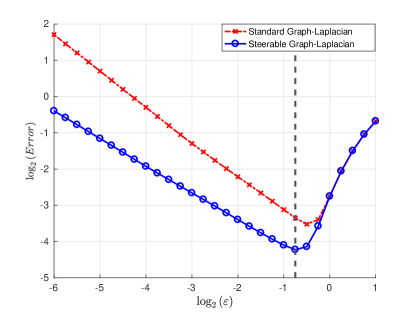
Figure 1: Errors in approximating $\Delta_{\mathcal{M}}f(x_{0})$ by the standard graph Laplacian (equations (1) and (2)) and by the steerable graph Laplacian (equation (28)) as a function of $\varepsilon$ (in $\log$ scale). The region to the left of the dashed vertical line is dominated by the variance error term, whereas the region to the right of the dashed vertical line is dominated by the bias error term.

Additionally, we computed the eigenvalues of $\tilde{L}$ as described in Section 2.3, and compared them with the eigenvalues of the standard (normalized) graph Laplacian. The results can be seen in Figure 2. It is evident that the eigenvalues in both cases agree with the well-known multiplicities of the spherical harmonics (the eigenfunctions of the Laplacian on the unit sphere). However, is clear that the eigenvalues of $\tilde{L}$ admit smaller fluctuations compared to the eigenvalues of the standard (normalized) graph Laplacian, owing to the improved convergence rate of $\tilde{L}$ to the Laplace-Beltrami operator.

Lastly, in Figure 3 we illustrate a single eigenfunction of the steerable graph Laplacian (computed via Theorem 3), corresponding to the indices $m=3,k=4$, where we used $N=512$ points and $\varepsilon=1$. The figure highlights the difference between the vector $\tilde{v}_{m,k}$ in (21) and the eigenfunction $\tilde{\Phi}_{m,k}$ itself. While the former is analogous to an eigenvector of the standard graph Laplacian (in the sense that it is defined only over the original data points), the latter extends its domain of definition by additionally assigning values to all rotations of the original data points (images). Note that the behavior of the eigenfunctions $\tilde{\Phi}_{m,k}$ over the orbits of the images’ rotations is given by Fourier modes, which is in agreement with the explicit formula for the spherical harmonics (given by Fourier modes in the azimuthal direction).

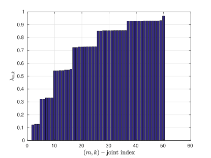
(a)

(b)

Figure 2: Eigenvalues of the steerable (left) and standard (right) normalized graph Laplacians, for $\varepsilon=1/4$ and $2,000$ data points sampled uniformly from the sphere. For the steerable graph Laplacian, the eigenvalues were sorted in ascending order and enumerated over $(m,k)$ using a single joint index.

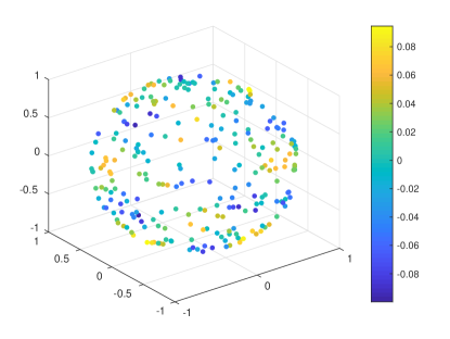
(a) $\tilde{v}_{m,k}$

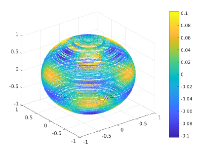
(b) $\tilde{\Phi}_{m,k}=\tilde{v}_{m,k}\cdot e^{\imath m\vartheta}$

Figure 3: An eigenfunction (real part only) of the steerable graph Laplacian $\tilde{L}$, corresponding to $m=3$ and $k=4$ (see Theorem 3), using $N=512$ points sampled uniformly from the sphere, and $\varepsilon=1$. On the left we show the values of the eigenfunction only for the original $512$ data points (given by the vector $\tilde{v}_{m,k}$ of (21)), and on the right we show all values of the eigenfunction $\tilde{\Phi}_{m,k}$, including the angular part (given explicitly by Fourier modes $e^{\imath m\vartheta}$) assigning values to all rotations of the original data points (visible as orbits in the shape of horizontal rings covering the sphere).

2.5 Filtering image datasets by the steerable manifold harmonics

Next, we propose to expand our dataset of images and all of their rotations by a carefully-chosen subset of the steerable manifold harmonics (the eigenfunctions of the steerable graph Laplacian $\tilde{L}$, see Theorem 3).

Consider the function $F_{m,\ell}\in\mathcal{H}$ given by

$$F_{m,\ell}(i,\varphi)=x_{i,(m,\ell)}^{\varphi},$$ (30)

where $x_{i,(m,\ell)}^{\varphi}$ stands for the $(m,\ell)$’th coordinate of the $i$’th data-point rotated by $\varphi$ (via (6)). In essence, the function $F_{m,\ell}$ describes the $(m,\ell)$’th coordinate of all points in the dataset and all of their rotations. As $F_{m,\ell}\in\mathcal{H}$, it can be expanded in the basis $\tilde{\Phi}$, and we can write

$$F_{m,\ell}=\sum_{m^{{}^{\prime}}=-\infty}^{\infty}\sum_{k=1}^{N}A_{({m^{{}^{\prime}},k}),({m,\ell})}\tilde{\Phi}_{m^{{}^{\prime}},k}$$ (31)

for all $(m,\ell)$ pairs, where $A_{({m^{{}^{\prime}},k}),({m,\ell})}$ are some associated expansion coefficients. We propose to “filter” the functions $F_{m,\ell}$ for each pair $(m,\ell)$ by considering a truncated expansion of the form of (31), with expansion coefficients obtained by solving

$$\min_{A}\left\|F_{m,\ell}-\sum_{m^{{}^{\prime}}=-M^{{}^{\prime}}}^{M^{{}^{\prime}}}\sum_{k=1}^{k_{m^{{}^{\prime}}}}A_{({m^{{}^{\prime}},k}),({m,\ell})}\tilde{\Phi}_{m^{{}^{\prime}},k}\right\|_{\mathcal{H}}^{2},$$ (32)

where $A$ is a matrix of expansion coefficients with rows indexed by $({m^{{}^{\prime}},k})$ and columns indexed by $({m,\ell})$.

As for the numbers of chosen basis functions $\left\{k_{m^{{}^{\prime}}}\right\}$ and $M^{{}^{\prime}}$, we propose the following natural truncation rule based on a cut-off frequency $\lambda_{c}\in\mathbb{R}_{+}$:

$$k_{m^{{}^{\prime}}}=\max\left\{k:\tilde{\lambda}_{m^{{}^{\prime}},k}<\lambda_{c}\right\},$$ (33)

where $\left\{\tilde{\lambda}_{m,k}\right\}$ are the eigenvalues (sorted in non-decreasing order w.r.t $k$) of the normalized steerable graph Laplacian $\tilde{L}$. Then, $M^{{}^{\prime}}$ is simply the largest $\left|m^{{}^{\prime}}\right|$ s.t. $k_{m^{{}^{\prime}}}>0$. Fundamentally, this truncation rule can be viewed as the analogue of the classical truncation of Fourier expansions. Figure 5 illustrates a typical configuration of index-pairs $(m^{{}^{\prime}},k)$ resulting from the truncation rule of (33).

We motivate the above-mentioned approach (series expansion and truncation rule) as follows. It is well known that for smooth and compact manifolds the Laplace-Beltrami operator $\Delta_{\mathcal{M}}$ admits a sequence of eigenvalues $\left\{\mu_{k}\right\}_{k=0}^{\infty}$ and eigenfunctions $\left\{\phi_{k}\right\}_{k=0}^{\infty}$, which are orthogonal and complete in the class of square-integrable functions on $\mathcal{M}$, denoted by $\mathcal{L}^{2}(\mathcal{M})$. Therefore, every function $f\in\mathcal{L}^{2}(\mathcal{M})$ can be expanded as

$$f(x)=\sum_{k=1}^{\infty}a_{k}\phi_{k}(x),\quad\quad a_{k}=\int_{\mathcal{M}}f(x){\phi_{k}^{*}}(x)dx.$$ (34)

In this context, it is possible to consider the coordinates of $\mathcal{M}$ in the ambient space, i.e. $x_{m,\ell}$ for every $x\in\mathcal{M}$, as smooth functions over $\mathcal{M}$, which can be approximated by truncating the above-mentioned expansion. In particular, we provide the following proposition, which bounds the error in approximating the coordinates of $\mathcal{M}$ using a truncated series of manifold harmonics.

Proposition 4.

Let $\left\{\phi_{k}\right\}_{k=1}^{\infty}$ and $\left\{\mu_{k}\right\}_{k=1}^{\infty}$ be the eigenfunctions and eigenvalues (sorted in non-decreasing order), respectively, of the negative-defined Laplace-Beltrami operator $\Delta_{\mathcal{M}}$. Then, we have that

$$\frac{1}{\operatorname{Vol}{\left\{\mathcal{M}\right\}}}\int_{\mathcal{M}}\left\|\sum_{k=1}^{n}c_{k}\phi_{k}(x)-x\right\|^{2}_{2}dx\leq\frac{d}{\mu_{n+1}},\quad\quad c_{k}=\int_{\mathcal{M}}x\phi_{k}^{*}(x)dx,$$ (35)

where $\operatorname{Vol}{\left\{\mathcal{M}\right\}}$ is the volume of $\mathcal{M}$, $d$ is the intrinsic dimension of $\mathcal{M}$, and $c_{k}\in\mathbb{C}^{\mathcal{D}}$ are the expansion coefficients of $x\in\mathbb{C}^{\mathcal{D}}$ (i.e. of every coordinate function of the embedded manifold) w.r.t $\phi_{k}$.

Proof.

The proof follows immediately from combining equation ($3.1$) in [1] and Proposition $3.1$ in [25]. ∎

It is important to note that by the properties of $\Delta_{\mathcal{M}}$ we have that $\mu_{n}{\rightarrow}\infty$ when $n\rightarrow\infty$ [28], and therefore we can get an arbitrarily small approximation error for the coordinates of $\mathcal{M}$ using a sufficiently large number of manifold harmonics. As we have shown in Section (2.3) that $\tilde{L}$ approximates the Laplace-Beltrami operator $\Delta_{\mathcal{M}}$, we follow the common practice and use the eigenfunctions and eigenvalues of $\tilde{L}$, i.e. $\left\{\tilde{\Phi}_{m,k}\right\}$ and $\left\{\tilde{\lambda}_{m,k}\right\}$, as discrete proxies for $\left\{\phi_{k}\right\}$ and $\left\{\mu_{k}\right\}$ in (35).

Next, we proceed to derive a simple and efficient solution to problem (32). By our construction of the Hilbert space $\mathcal{H}$, one can write (32) explicitly as

$$\min_{A}\left\{\sum_{i=1}^{N}\int_{0}^{2\pi}\left|x_{i,(m,\ell)}^{\varphi}-\sum_{m^{{}^{\prime}}=-M^{{}^{\prime}}}^{M^{{}^{\prime}}}\sum_{k=1}^{k_{m^{{}^{\prime}}}}A_{({m^{{}^{\prime}},k}),({m,\ell})}\tilde{\Phi}_{m^{{}^{\prime}},k}(i,\varphi)\right|^{2}d\varphi\right\},$$ (36)

which is interpreted as performing regression over the entire dataset of images and all of their planar rotations using the functions $\tilde{\Phi}_{m,k}$ restricted to $k\in\left\{1,\ldots,k_{m^{{}^{\prime}}}\right\},m\in\left\{-M^{{}^{\prime}},\ldots,M^{{}^{\prime}}\right\}$. Recall that by (6), we have that

$$x_{i,(m,\ell)}^{\varphi}=x_{i,(m,\ell)}e^{\imath m\varphi},$$ (37)

where $x_{i,(m,\ell)}$ stands for the $(m,\ell)$’th coordinate of the $i$’th data-point. It turns out that (36) can be significantly simplified by substituting (37) into (36) together with the steerable form of $\tilde{\Phi}_{m,\ell}$ (i.e. (21)), while making use of the orthogonality of the Fourier modes $\left\{e^{\imath m\varphi}\right\}_{m=-\infty}^{\infty}$ over $[0,2\pi)$. It then immediately follows that the matrix of coefficients $A$ in the solution of (36) is block-diagonal, where the blocks can be obtained by solving ordinary least-squares problems. In particular, we have that

$$A_{({m^{{}^{\prime}},k}),({m,\ell})}=\begin{dcases}B^{(m)}_{k,\ell},&m=m^{{}^{\prime}},\\ 0,&m\neq m^{{}^{\prime}},\end{dcases}$$ (38)

where $B^{(m)}$ is the $m$’th block on the diagonal of $A$, obtained by solving the least-squares system

$$\min_{B^{(m)}}\left\|X^{(m)}-\widetilde{V}^{(m)}B^{(m)}\right\|^{2}_{F},$$ (39)

where $\left\|\cdot\right\|_{F}$ stands for the Frobenius norm, and $X^{(m)}$ and $\widetilde{V}^{(m)}$ are given by

$$X^{(m)}=\begin{pmatrix}x_{1,(m,1)}&\ldots&x_{1,(m,\ell_{m})}\\ \vdots&\ddots&\vdots\\ x_{N,(m,1)}&\ldots&x_{N,(m,\ell_{m})}\end{pmatrix},\quad\quad\quad\widetilde{V}^{(m)}=\begin{pmatrix}|&&|\\ \tilde{v}_{m,1}&\cdots&\tilde{v}_{m,k_{m}}\\ |&&|\end{pmatrix},$$ (40)

with $\tilde{v}_{m,k}$ given by (21) and (22). We mention that $k_{m^{{}^{\prime}}}$ changes with the angular index $m^{{}^{\prime}}$, and in particular, is typically smaller for higher angular frequencies (larger $|m|$). Therefore, the size of the blocks $B^{(m)}$ reduces with $|m|$, as illustrated by Figure 5. Once the coefficients matrices $\left\{B^{(m)}\right\}$ were obtained by solving (39), we define

$$\hat{X}^{(m)}\triangleq\widetilde{V}^{(m)}B^{(m)}$$ (41)

as the filtered dataset corresponding to the angular index $m$.

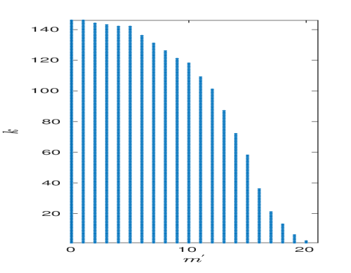
Figure 4: A typical configuration of index pairs $(m^{{}^{\prime}},k)$ obtained by the truncation rule of (33), for non-negative angular indices $m$.

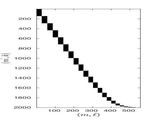
Figure 5: A typical structure of the matrix $A$ for non-negative angular indices $m$ and $m^{{}^{\prime}}$. Black-coloured regions correspond non-zero entries, where each block corresponds to a different angular index $m=m^{{}^{\prime}}$.

Lastly, a favorable interpretation of this procedure can be derived as follows. If we denote by $Q^{(m)}$ a matrix whose columns are orthonormal and span the columns of $\widetilde{V}^{(m)}$, then $\hat{X}^{(m)}$ can be written equivalently as

$$\hat{X}^{(m)}=Q^{(m)}\left[Q^{(m)}\right]^{*}X^{(m)}=C^{(m)}X^{(m)},$$ (42)

where $(\cdot)^{*}$ denotes complex-conjugate and transpose, and we defined the $N\times N$ “filtering” matrices

$$C^{(m)}\triangleq Q^{(m)}\left[Q^{(m)}\right]^{*},$$ (43)

which are applied to our dataset for every angular index separately. Essentially, $C^{(m)}$ acts as a “low-pass filter”, in the sense that it retains only the contribution of steerable manifold harmonics with low frequencies (i.e. eigenvalues below the threshold $\lambda_{c}$). In this context, the cut-off frequency $\lambda_{c}$ controls the rank of $C^{(m)}$, which is equal to $k_{m}$, and the degree to which $C^{(m)}$ suppresses oscillations in the data.

3 Algorithms summary and computational cost

We outline the algorithms for evaluating the steerable manifold harmonics and employing them for filtering image datasets in Algorithms 1 and 2, respectively. We note that two optional modifications to the procedure of evaluating the steerable manifold harmonics are proposed in Section 4 and Appendix F, respectively. The first modification is for improving the robustness of the procedure to noise, and was added to Algorithm 1 in step 4 under the label “Implicit debiasing (optional)”. The second modification, which is used for normalizing non-uniform sampling densities, was added to Algorithm 1 in step 6 under the label “Density normalization (optional)”.

Algorithm 1 Evaluating the steerable manifold harmonics

1:Required: A dataset of $N$ points $\left\{x_{1},\ldots,x_{N}\right\}\subset\mathbb{C}^{\mathcal{D}}$, where $x_{i,(m,\ell)}$ is the $(m,\ell)$’th coordinate of $x_{i}$ (see Section 2.1).

2:Choose a numerical-integration parameter $K$ (see (16)), and a Gaussian kernel parameter $\varepsilon$.

3:For every $1\leq i,j\leq N$, $k\in\left\{0,\ldots,K-1\right\}$, compute the affinities

$${W}_{i,j}^{(k)}=\exp{\left\{-{\left\|x_{i}-x_{j}^{(k)}\right\|^{2}}{/\varepsilon}\right\}},\quad\quad\quad x_{j,(m,\ell)}^{(k)}=x_{j,(m,\ell)}e^{\imath 2\pi mk/K}.$$ (44)

4: Implicit debiasing (optional): Set ${W}_{i,i}^{(k)}=0$ for $1\leq i\leq N$ and $k=0,\ldots,K-1$.

5: For every angular index $m=-M,\ldots,M$ and $1\leq i,j\leq N$, evaluate

$$\hat{W}_{i,j}^{(m)}=\frac{2\pi}{K}\sum_{k=0}^{K-1}{W}_{i,j}^{(k)}e^{\imath 2\pi mk/K},\quad\quad\quad D_{i}=\sum_{j=1}^{N}\hat{W}_{i,j}^{(0)}.$$ (45)

6: Density normalization (optional):

1. For every angular index $m=-M,\ldots,M$ update:

   $$\hat{W}^{(m)}\leftarrow D^{-1}\hat{W}^{(m)}D^{-1},$$ (46)

   where $D$ is a diagonal matrix with $\left\{D_{i}\right\}_{i=1}^{N}$ on its diagonal.

2. For every $i=1,\ldots,N$ update:

   $$D_{i}\leftarrow\sum_{j=1}^{N}\hat{W}_{i,j}^{(0)}.$$ (47)

7: For every angular index $m=-M,\ldots,M$ form the matrix

$$\tilde{S}_{m}=I-D^{-1}\hat{W}^{(m)},$$ (48)

and return its eigenvectors $\left\{\tilde{v}_{m,k}\right\}_{k=1}^{N}$ and eigenvalues $\left\{\tilde{\lambda}_{m,k}\right\}_{k=1}^{N}$.

Algorithm 2 Rotationally-invariant dataset filtering

1:Required:

1. A dataset of $N$ points $\left\{x_{1},\ldots,x_{N}\right\}\subset\mathbb{C}^{\mathcal{D}}$, where $x_{i,(m,\ell)}$ is the $(m,\ell)$’th coordinate of $x_{i}$ (see Section 2.1).

2. Eigenvectors $\left\{\tilde{v}_{m,1},\ldots,\tilde{v}_{m,N}\right\}_{m=-M}^{M}$ and eigenvalues $\left\{\tilde{\lambda}_{m,1},\ldots,\tilde{\lambda}_{m,N}\right\}_{m=-M}^{M}$ of $\left\{\tilde{S}_{m}\right\}_{m=-M}^{M}$ from Algorithm 1.

2:Choose a cut-off frequency $\lambda_{c}$.

3:For $m=-M,\ldots,M$ do

1. Compute $k_{m}=\max\left\{k:\tilde{\lambda}_{m,k}<\lambda_{c}\right\}$, and form the matrices $X^{(m)}$ and $\widetilde{V}^{(m)}$ of (40).

2. Estimate the coefficients matrix $B^{(m)}$ by solving the least squares system of (39).

3. Compute $\hat{X}^{(m)}=\widetilde{V}^{(m)}B^{(m)}.$

4:The filtered dataset is given by $\hat{X}=[\hat{X}^{(-M)}\cdots\hat{X}^{(M)}]$.

We now turn our attention to the computational complexity of Algorithms 1 and 2. We begin with Algorithm 1. The first step is to compute all affinity measures $W^{k}_{i,j}$, which can be evaluated efficiently by the FFT if we notice that

$$\left\|x_{i}-x_{j}^{(k)}\right\|^{2}=\left\|x_{i}\right\|^{2}_{2}+\left\|x_{j}\right\|^{2}_{2}-2\operatorname{Re}{\left\{\sum_{m=-M}^{M}c_{i,j}^{(m)}e^{-\imath 2\pi mk/K}\right\}},$$ (49)

where we defined

$$c_{i,j}^{(m)}=\sum_{\ell=1}^{\ell_{m}}x_{i,(m,\ell)}x_{j,(m,\ell)}^{*}.$$ (50)

Note that computing $c_{i,j}^{(m)}$ for all $i,j,m$ takes $O(N^{2}\mathcal{D})$ operations. Therefore, if we denote

$$\bar{M}=\max{\left\{M,K\right\}},$$ (51)

the computational complexity of this step is $O(N^{2}D+N^{2}\bar{M}\log{\bar{M}})$ when using the FFT to compute (49). In a similar fashion, computing $\hat{W}^{m}_{i,j}$ (of step 5) by the FFT takes $O(N^{2}\bar{M}\log{\bar{M}})$ operations. Lastly, forming the matrices $\left\{\tilde{S}_{m}\right\}_{m=-M}^{M}$ requires $O(MN^{2})$ operations, and evaluating its eigenvectors and eigenvalues takes $O(MN^{3})$ operations. Overall, the computational complexity of Algorithm 1 is therefore

$$O\left(MN^{3}+N^{2}(\mathcal{D}+\bar{M}\log{\bar{M}})\right).$$ (52)

In practice, it is often the case that only a small fraction of pairs of indices $(i,j)$ contributes significantly to $W_{i,j}^{k}$, since only images which are similar up to a planar rotation admit a non-negligible affinity (assuming that $\varepsilon$ is sufficiently small). Hence, it is often possible to zero-out the small values of $W_{i,j}^{k}$, allowing for cheaper sparse-matrix computations. Additionally, computing the eigen-decomposition in step 7 for large datasets (large $N$) may be accomplished more efficiently using randomized methods [17, 2].

As of Algorithm 2, in part (b) of step 3 we need to minimize $\left\|X^{(m)}-\widetilde{V}^{(m)}B^{(m)}\right\|^{2}_{F}$ over ${B^{(m)}}$, where $X^{(m)}$ is of dimension $N\times\ell_{m}$, $\widetilde{V}^{(m)}$ is $N\times k_{m}$, and $B^{(m)}$ is $k_{m}\times\ell_{m}$. For each angular index $m$, this amounts to solving $\ell_{m}$ least-squares problems (one for each column of $B^{(m)}$), each of size of size $N\times k_{m}$. Assuming that $N\geq k_{m}$ and using the QR factorization to solve least-squares, this part requires $O(k_{m}^{2}N+Nk_{m}\ell_{m}+k_{m}^{2}\ell_{m})$ operations for every angular index $m$, as we need $O(k_{m}^{2}N)$ operations to compute the QR decomposition of $V^{(m)}$ (which needs to be computed only once), $O(k_{m}\ell_{m}N)$ operations to apply $Q$ of the QR to $X^{(m)}$, and $O(k_{m}^{2}\ell_{m})$ operations to solve the resulting $\ell_{m}$ triangular systems. Then, since part (c) of step 3 takes $O(Nk_{m}\ell_{m})$ operations for each $m$, it follows that Algorithm 2 requires

$$O\left(\sum_{m=-M}^{M}k_{m}^{2}N+Nk_{m}\ell_{m}+k_{m}^{2}\ell_{m}\right)=O\left(MN\bar{k}^{2}+\mathcal{D}\bar{k}(N+\bar{k})\right)$$ (53)

operations, where $\bar{k}=\max_{m}{\left\{k_{m}\right\}}$. As typically $\bar{k}<<N$, the computational cost of Algorithm 2 is negligible compared to that of Algorithm 1.

4 Analysis under Gaussian noise

Next, we analyze our method under white Gaussian noise, and argue that in a certain sense the steerable graph Laplacian is robust to noise (after zeroing-out the diagonal of the steerable affinity operator ${W}$). Moreover, we argue that the filtering procedure (described in Section 2.5) allows us to reduce the amount of noise in the filtered dataset proportionally to the number of images $N$.

In this section, we consider the noisy data points

$$y_{i,(m,\ell)}=x_{i,(m,\ell)}+\eta_{i,(m,\ell)},$$ (54)

where $x_{i,(m,\ell)}$ is the $(m,\ell)$’th coordinate of the $i$’th clean data point, and $\left\{\eta_{i,(m,\ell)}\right\}$ are independent and normally distributed complex-valued noise variables with mean zero and variance $\sigma^{2}$ .

4.1 Noise robustness of the steerable graph Laplacian

We start by considering the effect of noise on the construction of $\tilde{L}$ (of (17)). Clearly, the noise changes the pairwise distances computed in $W_{i,j}(\vartheta,\varphi)$, where we note that from Theorem 3 and (13) it is sufficient to consider the effect of noise only on $D^{-1}_{i,i}W_{i,j}(0,\alpha)$, for all $\alpha\in[0,2\pi)$ and $i,j=1,\ldots,N$. To this end, consider the set of points $\mathcal{Y}_{i}^{\alpha}=\left\{y_{1}^{\alpha},\cdots,y_{i-1}^{\alpha},y_{i},y_{i+1}^{\alpha},\cdots,y_{N}^{\alpha}\right\}\subset\mathbb{C}^{\mathcal{D}}$, where all points except the $i$’th were replaced with their rotations by an angle $\alpha$ (via (6)). We have that

$$y_{j}^{\alpha}=x_{j}^{\alpha}+\eta_{j}^{\alpha},\quad\quad y_{j,(m,\ell)}^{\alpha}=x_{j,(m,\ell)}e^{\imath m\alpha}+\eta_{j,(m,\ell)}e^{\imath m\alpha},$$ (55)

for $j\neq i,\;j=1,\ldots,N$, and it is evident that the set of noise points $\left\{\eta_{1}^{\alpha},\cdots,\eta_{i-1}^{\alpha},\eta_{i},\eta_{i+1}^{\alpha},\cdots,\eta_{N}^{\alpha}\right\}$ are still i.i.d Gaussian. Then, Theorem $2.1$ (and specifically equation $(1)$) in [12], when applied to the set $\mathcal{Y}_{i}^{\alpha}$, asserts that if we denote $\gamma=\mathcal{D}\sigma^{2}$ and vary $\mathcal{D}$ and $\sigma^{2}$ such that $\gamma$ remains constant, then

$$W_{i,j}(0,\alpha)=\exp{\left\{-\left\|y_{i}-y_{j}^{\alpha}\right\|^{2}/\varepsilon\right\}}\underset{\mathcal{D}\rightarrow\infty}{\longrightarrow}\exp{\left\{-\left(\left\|x_{i}-x_{j}^{\alpha}\right\|^{2}+2\gamma\right)/\varepsilon\right\}}$$ (56)

in probability, for all $j\neq i$. Essentially, this result is due to the concentration of measure of high-dimensional Gaussian random vectors, and in particular the fact that $\left\{\eta_{i}^{\alpha}\right\}$ are uncorrelated and are concentrated around the surface of a sphere in $\mathbb{C}^{\mathcal{D}}$. Therefore, in the regime of high dimensionality and small noise-variance, the effect of the noise on the pairwise distances (between different data-points and rotations) is only an additive constant bias term. Note that even though the noise variance tends to zero, the overall noise magnitude $\gamma=\mathcal{D}\sigma^{2}$ is kept constant and may be large, corresponding to a low signal-to-noise ratio (SNR). We further mention that this constant-bias effect is not restricted to Gaussian white noise, as it occurs also when the noise admits a general covariance matrix $\Sigma$, and even when the noise takes other certain non-Gaussian distributions (see [12] for specific details and conditions).

Next, in order to correct for the bias in the distances, we follow [13] and zero-out the diagonal of $W$, that is, we update

$$W_{i,j}(0,\alpha)\leftarrow\begin{dcases}W_{i,j}(0,\alpha),&i\neq j,\\ 0,&i=j.\end{dcases}$$ (57)

Then, we expect $D^{-1}$ to correct (implicitly) for the bias in $W$, since

$$D_{i,i}= \sum_{j\neq i,j=1}^{N}\int_{0}^{2\pi}W_{i,j}(0,\alpha)d\alpha=\sum_{j\neq i,j=1}^{N}\int_{0}^{2\pi}\exp{\left\{-\left\|y_{i}-y_{j}^{\alpha}\right\|^{2}/\varepsilon\right\}}d\alpha$$

$$\underset{\mathcal{D}\rightarrow\infty}{\longrightarrow} e^{-2\gamma/\varepsilon}\sum_{j\neq i,j=1}^{N}\int_{0}^{2\pi}\exp{\left\{-\left\|x_{i}-x_{j}^{\alpha}\right\|^{2}/\varepsilon\right\}}d\alpha,$$ (58)

in probability, and thus

$$D^{-1}_{i,i}W_{i,j}(0,\alpha)\underset{\mathcal{D}\rightarrow\infty}{\longrightarrow}\frac{\exp{\left\{-\left\|x_{i}-x_{j}^{\alpha}\right\|^{2}/\varepsilon\right\}}}{\sum_{j\neq i,j=1}^{N}\int_{0}^{2\pi}\exp{\left\{-\left\|x_{i}-x_{j}^{\alpha^{{}^{\prime}}}\right\|^{2}/\varepsilon\right\}}d\alpha^{{}^{\prime}}}$$ (59)

in probability, which is equivalent to its clean counterpart for $i\neq j$ (after zeroing-out the diagonal). Lastly, we argue that zeroing-out the diagonal of $W$ does not change the point-wise convergence rate of the clean steerable graph Laplacian (as reported by Theorem 2), as it results in an error which is negligible compared to the leading error terms (see the end of Section E.2 in the proof of Theorem 2, and [31] for an analogous argument in the case of the standard graph Laplacian).

In Figure 6, we show the error in estimating $\Delta_{\mathcal{M}}f(x_{0})$ in a noisy high-dimensional counterpart of the numerical example of Section 2.4 (using the same setting of $N=2,000$ and the optimal choice $\varepsilon=2^{-0.75}$). To generate Figure 6, we embedded the unit sphere in increasing dimensions $\mathcal{D}$ (using a random orthogonal transformation) and added white Gaussian noise with variance $\sigma^{2}$ to each dimension, such that $\mathcal{D}\sigma^{2}=\gamma$ is kept fixed. We then compared the error in estimating $\Delta_{\mathcal{M}}f(x_{0})$ to the error obtained in the clean setting. Note that for the unit sphere the signal-to-noise ratio (SNR) is equal to $1/\gamma=1/(\mathcal{D}\sigma^{2})$. It is evident that as predicted by our analysis, the debiased steerable graph Laplacian converges to the clean steerable graph Laplacian in the regime of high dimensionality and small noise variance. Particularly, in the case of $SNR=10$ ($\gamma=0.1$), already for $\mathcal{D}=100$ the error resulting only from the noise becomes comparable to the approximation error in the clean setting. In the case of $SNR=1$ ($\gamma=1$), this happens roughly at $\mathcal{D}=1,000$.

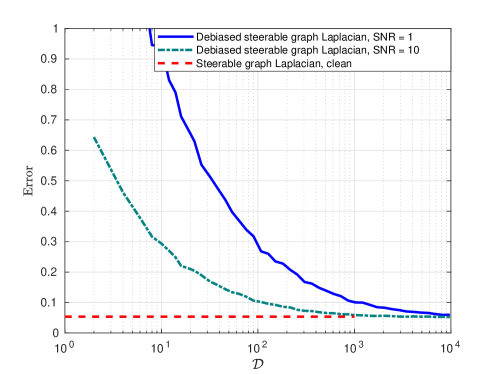
Figure 6: Errors in approximating the Laplace-Beltrami operator on the unit sphere (following the numerical example in Section 2.4) using the debiased steerable graph Laplacian constructed from noisy data points, as function of the ambient dimension $\mathcal{D}$. The debiased steerable graph Laplacian is computed using $\varepsilon=2^{-0.75}$ (which was optimal for the clean case) and $N=2,000$ noisy measurements, where the noise is additive white Gaussian with variance $\sigma^{2}$, while $SNR=1/(\mathcal{D}\sigma^{2})$ is kept fixed. The red dashed horizontal line corresponds to the error obtained from the clean steerable graph Laplacian in this setting (see Figure 1).

In summary, the analysis and numerical example in this section suggest that when the dimension $\mathcal{D}$ is large, the noise variance $\sigma^{2}$ is small, and the overall noise magnitude $\gamma=\mathcal{D}\sigma^{2}$ is fixed (and may be large compared to the magnitude of the signal), the steerable graph Laplacian constructed from the noisy data after implicit debiasing (by zeroing-out the diagonal of $W$) is expected to be close to its clean counterpart.

4.2 Performence of the filtering procedure

Next, we consider the eigenvectors and eigenvalues computed from the clean (normalized) steerable graph Laplacian, and analyze the effect of the filtering procedure (described in Section 2.5) on the noise in the dataset. From (42), the de-noised data for angular frequency $m$ is given by

$$\widetilde{X}^{(m)}=C^{(m)}Y^{(m)}=Q^{(m)}\left[Q^{(m)}\right]^{*}Y^{(m)},$$ (60)

where $Y^{(m)}$ is the matrix of noisy data points corresponding to angular index $m$, i.e. $Y^{(m)}_{i,\ell}=y_{i,(m,\ell)}$. Since $Q^{(m)}$ consists of $k_{m}$ orthonormal column vectors independent of the noise, and recalling that $\gamma=\mathcal{D}\sigma^{2}$, $\mathcal{D}=\sum_{m=-M}^{M}\ell_{m}$, we have that

$$\frac{1}{N}\mathbb{E}\left\|\hat{X}-\widetilde{X}\right\|^{2}_{F}=\frac{1}{N}\sum_{m=-M}^{M}\mathbb{E}\left\|\hat{X}^{(m)}-\widetilde{X}^{(m)}\right\|^{2}_{F}=\frac{\sigma^{2}\sum_{m=-M}^{M}k_{m}\ell_{m}}{N}\leq\max_{m}{\left\{k_{m}\right\}}\frac{\gamma}{N},$$ (61)

where $\hat{X}=[\hat{X}^{(-M)}\cdots\hat{X}^{(M)}]$ ($\hat{X}^{(m)}$ is defined in (42)) represents the clean filtered dataset, and $\widetilde{X}=[\widetilde{X}^{(-M)}\cdots\widetilde{X}^{(M)}]$ represents the noisy filtered dataset. Hence, larger datasets are expected to provide improved de-noising results, as the noise in the filtered dataset $\widetilde{X}$ reduces proportionally to $1/N$.

At this point, it is worthwhile to point out that the error bound of (61) is significantly better than what we would expect from using the standard graph Laplacian and its eigenvectors (to filter the coordinates of the dataset). Fundamentally, this is due to the block diagonal structure of the coefficients matrix $A$ (see Section 2.5), and more specifically, the fact that we only need to use eigenfunctions with angular index $m$ to expand data coordinates with the same angular index, in contrast to using all eigenfunctions. In particular, since the limiting operators of the steerable and standard graph Laplacians are the same (the Laplace-Beltrami operator), we expect the truncation rule of (33) to provide a similar number of eigenfunctions/eigenvectors from both methods. Then, if we were to use the eigenvectors of the standard graph Laplacian to filter our dataset, we would be required to use all $\sim\sum_{m=-M}^{M}k_{m}$ eigenvectors, and by a computation equivalent to (61) we would expect an error of $\sim\sum_{m=-M}^{M}k_{m}\frac{\gamma}{N}$, which is considerably larger than $\max_{m}{\left\{k_{m}\right\}}\frac{\gamma}{N}$. In conclusion, as the steerable graph Laplacian is more informative than the standard graph Laplacian, in the sense that it provides us with the angular part of each eigenfunction, it allows us to be more precise when filtering our dataset by matching the angular frequencies of the eigenfunctions to those of the data, thereby reducing the computational complexity and improving the de-noising performance considerably. This feature of the steerable graph Laplacian stands on its own, and is separate from the improved convergence rate to the Laplace-Beltrami operator (Theorem 2), which improves the accuracy of the eigenfunctions and eigenvalues compared to those of the standard graph Laplacian.

Lastly, we mention that the error term (61) can be viewed as a variance error term in a classical bias-variance trade-off, as we can write, conditioned on the clean dataset $X$, that

$$\frac{1}{N}\mathbb{E}\left\|{X}-\widetilde{X}\right\|^{2}_{F} =\frac{1}{N}\mathbb{E}\biggl{\|}{X}-\overbrace{\mathbb{E}\left[\widetilde{X}\right]}^{=\hat{X}}+\overbrace{\mathbb{E}\left[\widetilde{X}\right]}^{=\hat{X}}-\widetilde{X}\biggr{\|}^{2}_{F}$$

$$=\underbrace{\frac{1}{N}\mathbb{E}\left\|{X}-\hat{X}\right\|^{2}_{F}}_{\text{Bias}}+\underbrace{\frac{1}{N}\mathbb{E}\left\|\hat{X}-\widetilde{X}\right\|^{2}_{F}}_{\text{Variance}}.$$ (62)

Consequently, the overall error cannot get arbitrarily small, as there exists a bias term when approximating the clean data points by finitely many eigenfunctions (see Proposition 4). Therefore, in practice, the optimal de-noising results for a given dataset and noise variance would be attained as an optimum in a bias-variance trade-off, where a large cut-off frequency $\lambda_{c}$ would result in larger $\left\{k_{m}\right\}$ values and a larger variance error (as noise is mapped to more expansion coefficients), and a smaller cut-off frequency $\lambda_{c}$ would result in smaller $\left\{k_{m}\right\}$ values and a larger bias error.

Remark 4.

While the discussion in this section suggests that our method is robust to noise in the high-dimensional regime, it is not to say that reducing the dimensionality of a given dataset (with a given and fixed noise variance $\sigma^{2}$) would degrade the accuracy of the quantities computed by our method. On the contrary, a close examination of the results in [12] reveals that the errors in pairwise distances computed from noisy data points are dominated by $\sqrt{\mathcal{D}}\sigma^{2}$, meaning that projecting the data onto a lower-dimensional subspace (while retaining a sufficient approximation accuracy w.r.t the clean data) is encouraged – as it improves the accuracy of the pairwise affinities on one hand, and reduces the overall noise magnitude $\gamma=\mathcal{D}\sigma^{2}$ on the other.

5 Example: De-noising cryo-EM projection images

In this section, we demonstrate how we can use our framework to de-noise single-particle cryo-electron microscopy (cryo-EM) image datasets.

5.1 Cryo-EM

In single-particle cryo-EM [15, 7], one is interested in reconstructing a three-dimensional model of a macromolecule (such as a protein) from a set of two-dimensional images taken by an electron microscope. The procedure begins by embedding many copies of the macromolecule in a thin layer of ice, where due to the experimental set-up, the different copies are frozen at random unknown orientations. Then, an electron microscope acquires two-dimensional images of the these macromolecules (more precisely, it samples the Radon transform of the density function of the macromolecule). Consequently, it can be shown that the set of all projection images lies on a three-dimensional manifold diffeomorphic to the group SO(3). Thus, the manifold model assumption discussed in this work is natural for describing cryo-EM datasets. Note that due to the experimental set-up in cryo-EM, the in-plane rotation of each copy of the macromolecule is arbitrary, and therefore, so are the planar rotations of the two-dimensional images. Additionally, the images acquired in cryo-EM experiments are very noisy, with a typical SNR (Signal-to-Noise Ratio) of $1/10$ and lower. Simulated clean and noisy cryo-EM images of the 70S ribosome subunit can be seen in Figure 8 (top two rows).

5.2 De-noising recipe

Given a collection of cryo-EM projection images $\left\{I_{1},\ldots,I_{N}\right\}$ sampled on a Cartesian grid, we start by performing steerable principal components analysis (sPCA), as described in [21]. This procedure provides us with steerable basis functions (the steerable principal components) $\left\{\psi_{m,\ell}\right\}$ of the form of (3), which are optimal for expanding the images in the dataset and all of their rotations. For each basis function $\psi_{m,\ell}$, the steerable PCA also returns its associated eigenvalue $\nu_{m,k}$, which encodes the contribution of $\psi_{m,\ell}$ to the expansion (analogously to the eigenvalues of the covariance matrix in standard PCA). Therefore, we have that

$$I_{i}\approx\sum_{m=-M}^{M}\sum_{\ell=1}^{\ell_{m}}y_{i,(m,\ell)}\psi_{m,\ell},$$ (63)

where $y_{i,(m,\ell)}$ is the $(m,\ell)$’th expansion coefficient of the $i$’th image (provided by sPCA, see [21] for appropriate error bounds associated with (63)). Expanding the image dataset using such basis functions allows us to apply our filtering scheme in the domain of the expansion coefficients, as required by our algorithms. We note that for images corrupted by additive white Gaussian noise, the noise variance $\sigma^{2}$ is estimated from the corners of the images (where no molecule is expected to be present), and the number of basis functions used in the expansion, governed by $M$ and $\left\{\ell_{m}\right\}$, is determined by estimating which eigenvalues $\nu_{m,k}$ are above the noise level (i.e. exceed the Baik-Ben Arous-Péché transition point [3], see also [42, 41]) via

$$\ell_{m}=\max\left\{\ell:\;\nu_{m,\ell}>\sigma^{2}\left(1+\sqrt{\frac{n_{m}}{N}}\right)^{2}\right\},$$ (64)

where $\left\{n_{m}\right\}$ can be found in [21] ($n_{m}$ is the size of the $m$’th block in the block-diagonal covariance matrix associated with steerable PCA), and assuming that $\left\{\nu_{m,k}\right\}_{k}$ are sorted in a non-increasing order for every $m$. Correspondingly, $M$ in (63) is simply the largest $\left|m\right|$ s.t. $\ell_{m}>0$.

Using the above setting, the task of de-noising the images $\left\{I_{i}\right\}$ is reduced to the task of de-noising the sPCA coefficients $\left\{y_{i,(m,\ell)}\right\}$. We then estimate the steerable manifold harmonics $\left\{\tilde{v}_{m,k}\right\}$ (as described by Algorithm 1) from the dataset $\left\{y_{i}\right\}_{i=1}^{N}$, and follow by employing $\left\{\tilde{v}_{m,k}\right\}$ for filtering the dataset according to Algorithm 2. After obtaining the de-noised expansion coefficients $\left\{\hat{x}_{i,(m,\ell)}\right\}$, we can plug them back in the expansion (3) to get de-noised images. The procedure is summarized in Figure 7. Note that since $\left\{I_{i}\right\}$ are real-valued images, their expansion coefficients satisfy the symmetry

$$y_{i,(-m,\ell)}=y_{i,(m,\ell)}^{*}.$$ (65)

Therefore, it is sufficient to de-noise only the coefficients with non-negative angular frequencies.

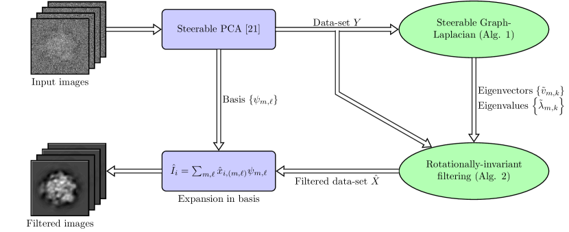
Figure 7: Schematic view of the de-noising procedure. We start by applying the steerable PCA [21] to the input images, obtaining basis functions $\left\{\psi_{m,\ell}\right\}$ and associated expansion coefficients $\left\{y_{i,(m,\ell)}\right\}$ (organized into the matrix $Y$ following the layout of (4)), where the truncation of the expansion is due to (64). Then, the dataset $Y$ is used to construct the steerable graph Laplacian, whose eigenfunctions (the steerable manifold harmonics) are obtained via Algorithm 1 with implicit debiasing (step 4) and without denisty normalization (step 6). Using the steerable manifold hamronics, we filter the dataset via Algorithm 2, and use the filtered coefficients $\left\{\hat{x}_{i,(m,\ell)}\right\}$ in conjunction with the basis functions $\left\{\psi_{m,\ell}\right\}$ to get back the filtered images.

5.3 Experimental results

We demonstrate the de-noising performance of our approach using simulated images of the 70S ribosome, of size $128\times 128$ pixels, after applying a filter to all images corresponding to a typical Contrast Transfer Function (CTF) [15] of the electron microscope. As described previously, we first map all images to their sPCA coefficients via [21] (with $T=10$ and half-Nyquist bandlimit), and then proceed according to our filtering scheme (Algorithms 1 and 2). We mention that throughout our experiments the choice $K=256$ was found satisfactory, and that $\varepsilon$ and $\lambda_{c}$ were chosen automatically for every experimental set-up (determined by the number of images $N$ and noise variance $\sigma^{2}$) as described in Appendix A. In every experiment, we compare the de-noised images resulting from our method to the images obtained directly from the sPCA coefficients (i.e. images computed from the coefficients $\left\{y_{i,(m,\ell)}\right\}$), and to images obtained after applying a shrinkage to the sPCA coefficients via $y_{i,(m,\ell)}w_{m,\ell}$, where the weights $\left\{w_{m,1},\ldots,w_{m,\ell_{m}}\right\}_{m=-M}^{M}$, which were computed as described in [42], correspond to the asymptotically-optimal Wiener filter [33]. Essentially, this is the optimal filter for the expansion coefficients in the sense of minimizing the mean squared error.

First, we demonstrate our method on $10,000$ projection images at signal-to-noise ratio of $1/20$. The de-noised images can be seen in Figure 8, where it is visually evident that the final de-noised images using our method contain many more details compared to sPCA Wiener filtering, which results in somewhat blurred images due to the aggressive shrinkage of sPCA coefficients. In terms of performance measures, our method (which we term “sMH filtering”, where sMH stands for “steerable manifold harmonics”) results in an average peak-SNR (pSNR) of $25.37$dB, where the sPCA Wiener filter provided $21.17$dB pSNR, and sPCA alone resulted in $17.64$dB pSNR.

It is therefore evident that Wiener filtering of sPCA coefficients is far from optimal in terms of de-noising and image recovery, as it essentially applies a single linear operator on the individual images, which is only optimal when the data resides on a linear subspace. However, in the case of cryo-EM, as the data resides on a manifold, it is reasonable to apply non-linear methods which account for the geometry and topology of the manifold. In this respect, our method is able to make use of all images and their rotations simultaneously to accurately estimate the structure of the manifold, and thereby provides an improved de-noising of the image dataset.

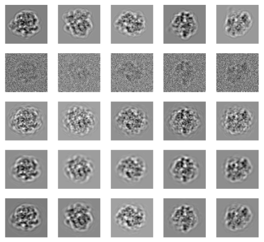
Figure 8: Images after de-noising, for $N=10,000$ and SNR $=1/20$. Different colummns correspond to different images from the dataset (different in-plane rotations and viewing directions of the molecule), while different rows correspond to (from top to bottom): clean images, noisy images, sPCA (pSNR $=17.64$dB), sPCA Wiener filter (pSNR $=21.17$dB), and sMH filtering (this paper, pSNR $=25.37$dB).

Next, Figure 9 demonstrates the performance of our method for SNR $=1/10$ and different values of $N$ (dataset size). As anticipated, our method is able to exploit larger datasets for improved de-noising, whereas the sPCA Wiener filtering offers only a mild gain beyond $2,000$ images. The reason for that is that the Wiener filtering is applied to each image separately, and therefore reaches saturation once the estimation of the sPCA from the noisy data is sufficiently accurate (approaches the sPCA of the clean data). Note that the pSNR from the projection onto the sPCA components (without shrinkage) reduces with $N$, because more basis functions $\psi_{m,\ell}$ are chosen (according to (64)) as $N$ increases, even if their contribution to expanding the dataset is negligible. Therefore, the dimension $\mathcal{D}$ increases, and with it also the overall noise magnitude $\mathcal{D}\sigma^{2}$. It is important to mention that even though the variance error term in (61) behaves like $1/N$, the improvement in the pSNR of our method is not expected to follow this trend, since the overall error also includes a bias error term (see (62)), such that the minimal error for every value of $N$ is attained as a different optimum in the bias-variance trade-off.

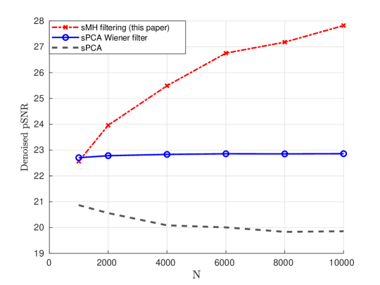
Figure 9: pSNR of de-noised images for SNR $=1/10$ and different dataset sizes $N$.

Lastly, we evaluated the de-noising quality for $N=10,000$ images and varying amounts of noise. The results are displayed in Figure 10, where we can see that our method outperforms the sPCA Wiener filter considerably in a wide range of SNRs. We remark that as the SNR decreases the asymptotics considered in Section 4 become less valid, thus at some point the steerable graph Laplacian becomes too noisy, and the performance gain of our method drops. This phenomenon is mostly evident for SNRs below $-14$dB, and our method eventually under-performs the sPCA Wiener filter at $-20$dB SNR.

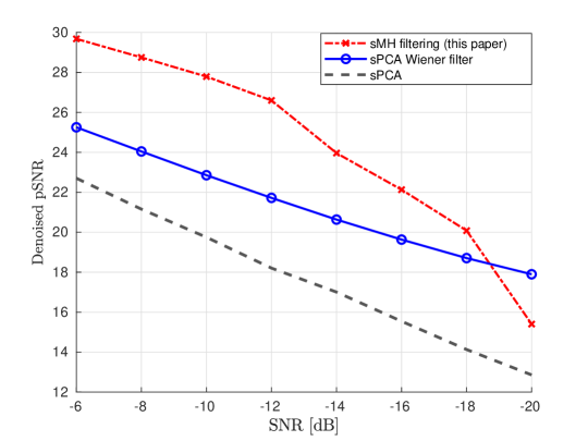
Figure 10: pSNR of de-noised images for $N=10,000$ and various SNR levels.

6 Conclusions and discussion

In this work, we introduced the steerable graph Laplacian, which generalizes the standard graph Laplacian by incorporating all planar rotations of all images in the dataset. We demonstrated that the (normalized) steerable graph Laplacian is both more accurate and more informative than the standard graph Laplacian, in the sense that it allows for an improved approximation of the Laplace-Beltrami operator on one hand, and admits eigenfunctions with a closed-form analytic expression of their angular part (i.e. the angular Fourier modes) on the other. This closed-form expression is essentially what allows for the efficient filtering procedure of the data coordinates (see Section 2.5), as we only need to estimate a block-diagonal coefficients matrix. Then, we have shown that under a suitable modification, the (normalized) steerable graph Laplacian is robust to noise in the regime of high dimensionality due to the concentration of measure of Gaussian noise. Moreover, we have seen that the proposed filtering procedure reduces the noise proportionally to the number of images in the dataset, which was corroborated by the experiments of de-noising cryo-EM projection images, where we demonstrated that our method can provide excellent de-noising results on highly noisy image datasets.

It is interesting to point-out that the steerable graph Laplacian, while utilized for filtering image datasets, can be employed for many other purposes. One application immediately coming to mind is the filtering of datasets consisting of periodic signals (see last remark in Section 2.1). However, and more importantly, the steerable graph Laplacian can replace the standard graph Laplacian in all applications where the domain is known to be rotationally-invariant (by our definition in Section 2.1). For instance, it can be used for regularization over general signal/data recovery inverse problems, or for dimensionality reduction in the framework of Diffusion Maps [8] and Laplacian Eigenmaps [4]. In this context, we mention the method of Vector Diffusion Maps (VDM) [32], which allows for diffusion-based dimensionality reduction for manifold data in the presence of nuisance parameters (such as planar rotations). However, as VDM computes the group ratios only between pairs of data points (e.g. optimal rotational alignments), it may be of interest to compare it to the steerable graph Laplacian, which essentially considers all planar rotations of all images. Lastly, we note that a possible future research direction is the extension of our techniques to other group actions (such as SO(3)).

Appendix A Choosing $\varepsilon$ and $\lambda_{c}$

In this section, we provide some guidelines on how to choose the parameters $\varepsilon$ and $\lambda_{c}$, and propose a method for determining them automatically.

In the clean setting, it is reasonable to choose the optimal value of $\varepsilon$ by minimizing the bias-variance error related to the convergence of the steerable graph Laplacian (i.e. equation (18)). However, in general this cannot be achieved without prior knowledge on geometrical quantities of $\mathcal{M}$, such as its curvature (see [31] and the related discussion therein). Nonetheless, methods for automatic picking of $\varepsilon$ for the standard graph Laplacian were proposed (see for example [9]). Unfortunately, such methods cannot be applied to noisy data in a straightforward manner, due to the effects of noise on the pairwise distances, and we are not aware of any work detailing the automatic choice of $\varepsilon$ for this case. We note however, that when the distances are computed from the noisy data-points $\left\{y_{1},\ldots,y_{N}\right\}$, and if $N$ is sufficiently large such that the noise is the dominant factor in determining $\varepsilon$, then it is reasonable to choose

$$\varepsilon\propto\sqrt{\mathcal{D}}\sigma^{2},$$ (66)

as this expression dominates the standard deviation of the errors in the pairwise (squared) distances (see [12] and analysis therein), and so can be used to set a region in which it is likely to find the optimal $\varepsilon$.

In order to find the optimal $\varepsilon$ and cut-off frequency $\lambda_{c}$ for a given dataset, we propose to use a cross-validation procedure. In particular, we choose $\varepsilon$ and $\lambda_{c}$ such that the log-likelihood of a noisy set of points, given a de-noised set (where the sets are disjoint), is maximized. In more detail, suppose that $\left\{y_{1},\ldots,y_{N}\right\}$ is a collection of noisy data-points as in (54), i.e.

$$y_{i}=x_{i}+\eta_{i},$$ (67)

where $\eta_{i}\in\mathbb{C}^{\mathcal{D}}$ are i.i.d Gaussian vectors with mean zero and covariance $\sigma^{2}I$, and $x_{i}$ are sampled from the manifold $\mathcal{M}$ with uniform distribution. Then, the log-likelihood of obtaining the subset $\left\{y_{N^{{}^{\prime}}+1},\ldots,y_{N}\right\}$, where $N^{{}^{\prime}}<N$, is given (up to additive constants) by

$$\sum_{i={N^{{}^{\prime}}+1}}^{N}\log\left[\frac{1}{\operatorname{Vol}\left\{\mathcal{M}\right\}}\int_{\mathcal{M}}\exp{\left\{-\left\|y_{i}-x\right\|^{2}/2\sigma^{2}\right\}}dx\right].$$ (68)

We then propose to approximate this log-likelihood by Monte-Carlo integration via the points

$$\left\{\hat{x}_{1}(\varepsilon,\lambda_{c}),\ldots,\hat{x}_{N^{{}^{\prime}}}(\varepsilon,\lambda_{c})\right\},$$ (69)

obtained from the de-noising of $\left\{y_{1},\ldots,y_{N^{{}^{\prime}}}\right\}$ using the parameters $(\varepsilon,\lambda_{c})$. That is, we define the empirical log-likelihood of $\left\{y_{N^{{}^{\prime}}+1},\ldots,y_{N}\right\}$ (as a function of the parameters $\varepsilon$ and $\lambda_{c}$) by

$$J(\varepsilon,\lambda_{c})=\sum_{i={N^{{}^{\prime}}+1}}^{N}\log{\left[\sum_{j=1}^{N^{{}^{\prime}}}\frac{2\pi}{K}\sum_{k=0}^{K-1}\exp{\left\{-\left\|y_{i}-\hat{x}^{2\pi k/K}_{j}(\varepsilon,\lambda_{c})\right\|^{2}/2\sigma^{2}\right\}}\right]},$$ (70)

where $\hat{x}^{2\pi k/K}_{j}(\varepsilon,\lambda_{c})$ stands for the rotation of $\hat{x}_{j}(\varepsilon,\lambda_{c})$ by an angle of $2\pi k/K$ according to (6). We mention that summing over the rotations improves the accuracy of the Monte-Carlo integration, as we account for one of the dimensions of the manifold $\mathcal{M}$ in the integration. Finally, we choose the parameters $\varepsilon$ and $\lambda_{c}$ by maximizing $J$, i.e.

$$\left\{\varepsilon^{opt},\lambda_{c}^{opt}\right\}=\operatorname*{arg\,max}_{(\varepsilon,\lambda_{c})}{\left\{J(\varepsilon,\lambda_{c})\right\}}.$$ (71)

Essentially, we expect the realizations of the noisy data-points $\left\{y_{N^{{}^{\prime}}+1},\ldots,y_{N}\right\}$ to be best explained when the de-noised points $\left\{\hat{x}_{1}(\varepsilon,\lambda_{c}),\ldots,\hat{x}_{N^{{}^{\prime}}}(\varepsilon,\lambda_{c})\right\}$ (and their rotations) lay as close as possible to $\mathcal{M}$, and we seek the best parameters for achieving that. For example, if we take $\lambda_{c}$ to be too small, then the de-noising error will be dominated by a bias term as we did not take a sufficient number of components to represent the features of the clean images accurately. Therefore we would expect the empirical log-likelihood to be small as the de-noised images will not be close to $\mathcal{M}$. On the other hand, if we take $\lambda_{c}$ to be too large, then over-fitting will occur, in the sense that some features of the noise will be preserved in the de-noised images. In that case, as the empirical likelihood is computed on a set independent from the set of de-noised points, we would again expect the empirical log-likelihood to be small.

Appendix B Quadratic form of $L$

In what follows, we derive the quadratic form of $L$ appearing in equation (12). First, for $f=\left[f_{1}(\vartheta),\ldots,f_{N}(\vartheta)\right]^{T}$ we have that

$$(Lf)(i,\vartheta)=D_{i,i}f_{i}(\vartheta)-\sum_{j=1}^{N}\int_{0}^{2\pi}W_{i,j}(\vartheta,\varphi)f_{j}(\varphi)d\varphi,$$ (72)

and therefore

$$\left\langle f,Lf\right\rangle_{\mathcal{H}}=\sum_{i=1}^{N}D_{i,i}\int_{0}^{2\pi}\left|f_{i}(\vartheta)\right|^{2}d\vartheta-\sum_{i,j=1}^{N}\int_{0}^{2\pi}\int_{0}^{2\pi}f_{i}^{*}(\vartheta)W_{i,j}(\vartheta,\varphi)f_{j}(\varphi)d\vartheta d\varphi.$$ (73)

Then, if we notice that

$$D_{i,i}=\sum_{j=1}^{N}\int_{0}^{2\pi}W_{i,j}(0,\alpha)d\alpha=\sum_{j=1}^{N}\int_{0}^{2\pi}W_{i,j}(\vartheta,\varphi)d\varphi$$ (74)

for every $\vartheta\in[0,2\pi)$ (by changing the integration parameters), we have that

$$\sum_{i=1}^{N}D_{i,i}\int_{0}^{2\pi}\left|f_{i}(\vartheta)\right|^{2}d\vartheta=\sum_{i,j=1}^{N}\int_{0}^{2\pi}\int_{0}^{2\pi}W_{i,j}(\vartheta,\varphi)\left|f_{i}(\vartheta)\right|^{2}d\vartheta d\varphi=\sum_{i,j=1}^{N}\int_{0}^{2\pi}\int_{0}^{2\pi}W_{i,j}(\vartheta,\varphi)\left|f_{j}(\varphi)\right|^{2}d\vartheta d\varphi,$$ (75)

due to the symmetry $W_{i,j}(\vartheta,\varphi)=W_{j,i}(\varphi,\vartheta)$ (see the definition of $W$ in (9)). Finally, using (75) we can write

$$\left\langle f,Lf\right\rangle_{\mathcal{H}} =\frac{1}{2}\sum_{i,j=1}^{N}\int_{0}^{2\pi}\int_{0}^{2\pi}W_{i,j}(\vartheta,\varphi)\left[\left|f_{i}(\vartheta)\right|^{2}+\left|f_{j}(\varphi)\right|^{2}-f_{i}(\vartheta)f_{j}^{*}(\varphi)-f_{i}^{*}(\vartheta)f_{j}(\varphi)\right]d\vartheta d\varphi$$

$$=\frac{1}{2}\sum_{i,j=1}^{N}\int_{0}^{2\pi}\int_{0}^{2\pi}W_{i,j}(\vartheta,\varphi)\left|f_{i}(\vartheta)-f_{j}(\varphi)\right|^{2}d\vartheta d\varphi.$$ (76)

Appendix C Linear rotationally-invariant operators

We start with the following definition of linear rotationally-invariant operators over $\mathcal{H}$.

Definition 5 (LRI operators).

An operator $G:\mathcal{H}\rightarrow\mathcal{H}$ is linear rotationally-invariant (LRI) over $\mathcal{H}$, if

1. For any fixed $(i,\vartheta)\in\Gamma$ (where $\Gamma$ defined in Section 2.2), the functional $\left\{Gf\right\}(i,\vartheta)$ is linear and continuous in $f$.

2. $G$ satisfies

   $$\left\{Gf\right\}(i,\vartheta-\alpha)=\left\{Gf^{\alpha}\right\}(i,\vartheta),\quad\quad f^{\alpha}(i,\vartheta)\triangleq f_{i}(\vartheta-\alpha),$$ (77)

   for all $f\in\mathcal{H}$, $\alpha\in[0,2\pi)$, and $(i,\vartheta)\in\Gamma$.

In the first requirement of Definition 5, the continuity property essentially means that if $f_{1}$ and $f_{2}$ are close (in $\mathcal{H}$), then $Gf_{1}(i,\vartheta)$ and $Gf_{2}(i,\vartheta)$ are also close (in absolute value). As for the second requirement (rotational-invariance), loosely speaking, it means that shifting the output of the operator cyclically by an angle $\alpha$ is equivalent to shifting the input by $\alpha$, hence the action of the operator itself does not depend on the angle $\vartheta$ (of $(i,\vartheta)\in\Gamma$). We mention that this property of linearity and rotational-invariance can be viewed as analogous to that of Linear-Time Invariant (LTI) operators, native to classical signal processing.

Remark 5.

Our definition of LRI operators is somewhat more restrictive than the name suggests (compared also to classical LTI operators) because of our requirement for continuity of every functional $\left\{G\cdot\right\}(i,\vartheta)$. We note that while this requirement can be removed, allowing for a broader class of operators, it is simpler to handle and sufficient for our purposes.

The next lemma characterizes the form of LRI operators explicitly.

Lemma 6 (Explicit form of LRI operators).

Let $G$ be an LRI operator over $\mathcal{H}$. Then, there exist unique $\left\{G_{i,j}\right\}_{i,j=1}^{N}\in\mathcal{L}^{2}(\mathbb{S}^{1})$, s.t. for any $f\in\mathcal{H}$ and $(i,\vartheta)\in\Gamma$

$$\left\{Gf\right\}(i,\vartheta)=\sum_{j=1}^{N}\int_{0}^{2\pi}G_{i,j}(\varphi-\vartheta)f_{j}(\varphi)d\varphi.$$ (78)

Proof.

By the Riesz representation theorem, if $\left\{G\cdot\right\}(i,\vartheta)$ is a linear and continuous functional over $\mathcal{H}$, then there exists a unique $g_{(i,\vartheta)}\in\mathcal{H}$ such that

$$\left\{Gf\right\}(i,\vartheta)=\left\langle g_{(i,\vartheta)},f\right\rangle_{\mathcal{H}}=\sum_{j=1}^{N}\int_{0}^{2\pi}g^{*}_{i,j}(\vartheta,\varphi)f_{j}(\varphi)d\varphi,$$ (79)

where $g_{(i,\vartheta)}\triangleq\left[g_{i,1}(\vartheta,\cdot),\ldots,g_{i,N}(\vartheta,\cdot)\right]^{T}$. Additionally, from (77), we have that

$$\left\{Gf\right\}(i,\vartheta)=\left\{Gf\right\}(i,\vartheta+\alpha-\alpha)=\left\{Gf^{\alpha}\right\}(i,\vartheta+\alpha)=\sum_{j=1}^{N}\int_{0}^{2\pi}g^{*}_{i,j}(\vartheta+\alpha,\varphi^{{}^{\prime}}+\alpha)f_{j}(\varphi^{{}^{\prime}})\varphi^{{}^{\prime}},$$ (80)

when changing the integration parameter via $\varphi^{{}^{\prime}}=\varphi-\alpha$. Lastly, taking $\alpha=-\vartheta$ and defining $G_{i,j}(\varphi-\vartheta)=g^{*}_{i,j}(0,\varphi-\vartheta)$ concludes the proof. ∎

The main contribution of Lemma 6 is to point out that every LRI operator can be characterized by a finite number of functions $\left\{G_{i,j}\right\}_{i,j=1}^{N}$ which can be expanded in a Fourier series. Therefore, $G$ can be mapped to (and described by) a sequence of matrices $\left\{\hat{G}^{(m)}\right\}_{m=-\infty}^{\infty}$ defined by

$$\hat{G}^{(m)}_{i,j}=\int_{0}^{2\pi}G_{i,j}(\alpha)e^{\imath m\alpha}d\alpha.$$ (81)

It is important to notice that from (6) and (9), it immediately follows that the steerable affinity operator $W$ of (9) is LRI with $G_{i,j}=W_{i,j}(0,\vartheta-\varphi)$. However, we note that for any fixed $(i,\vartheta)\in\Gamma$, it is evident that $Df(i,\vartheta)$ (where $D$ is the diagonal matrix defined in (11)) is not a continuous functional of $f$ (in $\mathcal{H}$), as small perturbations in $f$ may lead to arbitrarily large changes in $Df(i,\vartheta)$ as it depends on point-wise values of $f$. Therefore, the steerable graph Laplacian $L$ (from (11)) is not LRI. Nonetheless, as we shall see next, we can still employ the properties of LRI operators to characterize a broader family of operators, which includes the steerable affinity operator $W$ and the steerable graph Laplacian $L$ as special cases, with eigenfunctions admitting a particularly convenient form. This is the subject of the next proposition.

Proposition 7.

Consider an operator $H:\mathcal{H}\rightarrow\mathcal{H}$ of the form

$$H=A+G,$$ (82)

where $G$ is LRI and $A\in\mathbb{C}^{N\times N}$ is a complex-valued matrix. If $(\lambda,v)$ is an eigenvalue-eigenvector pair of the matrix

$$\hat{H}^{(m)}=A+\hat{G}^{(m)},$$ (83)

where $\hat{G}^{(m)}$ is from (81), then $\Phi=v\cdot e^{\imath m\vartheta}$ is an eigenfunction of $H$ with eigenvalue $\lambda$.

Proof.

The proof follows directly from Lemma 6 and the Fourier expansion of $G_{i,j}$. Let us write

$$\left\{H\Phi\right\}(i,\vartheta)=\sum_{j=1}^{N}A_{i,j}\Phi(j,\vartheta)+\sum_{j=1}^{N}\int_{0}^{2\pi}G_{i,j}(\varphi-\vartheta)\Phi(j,\varphi)d\varphi,$$ (84)

where we have used the explicit form of the LRI operator $G$ given by (78). Then, if we expand $G_{i,j}(\cdot)$ in a Fourier series as

$$G_{i,j}(\varphi-\vartheta)=\frac{1}{2\pi}\sum_{m=-\infty}^{\infty}\hat{G}_{i,j}^{(m)}e^{-\imath m(\varphi-\vartheta)},\quad\quad\hat{G}^{(m)}_{i,j}=\int_{0}^{2\pi}G_{i,j}(\alpha)e^{\imath m\alpha}d\alpha,$$ (85)

we have that

$$\left\{H\Phi\right\}(i,\vartheta)=\sum_{j=1}^{N}A_{i,j}\Phi(j,\vartheta)+\sum_{j=1}^{N}\frac{1}{2\pi}\sum_{m^{{}^{\prime}}=-\infty}^{\infty}\hat{G}_{i,j}^{m^{{}^{\prime}}}e^{\imath m^{{}^{\prime}}\vartheta}\int_{0}^{2\pi}\Phi(j,\varphi)e^{-\imath m^{{}^{\prime}}\varphi}d\varphi.$$ (86)

Therefore, by substituting $\Phi(i,\vartheta)=v_{i}e^{\imath m\vartheta}$, where $v_{i}$ stands for $i$’th element of $v$, we get

$$\left\{H\Phi\right\}(i,\vartheta)=e^{\imath m\vartheta}\sum_{j=1}^{N}A_{i,j}v_{j}+e^{\imath m\vartheta}\sum_{j=1}^{N}\hat{G}_{i,j}^{m}v_{j},$$ (87)

where we have used the orthogonality of $\left\{e^{\imath m\vartheta}\right\}_{m=-\infty}^{\infty}$ over $[0,2\pi)$. Finally, it follows that

$$H\Phi=\left[(A+\hat{G}^{(m)})v\right]e^{\imath m\vartheta}=\lambda ve^{\imath m\vartheta}=\lambda\Phi,$$ (88)

since $v$ is an eigenvector of $A+\hat{G}^{(m)}$ with eigenvalue $\lambda$. ∎

Therefore, even though the steerable graph Laplacian $L$ is not strictly LRI according to Definition 5, it still takes the form of the operators considered in Proposition 7, and consequently, we can derive its eigen-decomposition by making use of the sequence of matrices $\left\{\hat{W}^{(m)}\right\}_{m=-\infty}^{\infty}$ of (13).

Appendix D Proof of Theorem 1

Proof.

First, we note that by (15) and (9), it follows directly that $\hat{W}^{(m)}$ is Hermitian, which implies that $S_{m}$ is also Hermitian, and therefore can be diagonalized by a set of orthogonal eigenvectors. Next, as $L$ is of the form $A+G$ as required by Proposition 7 (where $A$ is a matrix and $G$ is an LRI operator), we can obtain a sequence of eigenfunctions and eigenvalues of $L$ by diagonalizing the matrices $S_{m}=D-\hat{W}^{(m)}$ for every $m\in\mathbb{Z}$. Then, the eigenvalues $\left\{\lambda_{m,k}\right\}_{k=1}^{N}$ must be real-valued (since $S_{m}$ is Hermitian), and moreover, by the quadratic form of $L$ (12) it follows that $\left\langle f,Lf\right\rangle_{\mathcal{H}}\geq 0$, which implies that $L$ is semi-positive definite and thus the eigenvalues $\left\{\lambda_{m,k}\right\}_{k=1}^{N}$ are non-negative.

Lastly, the fact that $\left\{\Phi_{m,k}\right\}_{m,k}$ are orthogonal and complete follows from the orthogonality and completeness of $\left\{e^{\imath m\vartheta}\right\}_{m=-\infty}^{\infty}$ over $\mathcal{L}^{2}(\mathbb{S}^{1}),$ and the orthogonality and completeness of $\left\{v_{m,k}\right\}_{k=1}^{N}$ over $\mathbb{C}^{N}$ (since $D-\hat{W}_{m}$ is Hermitian) for every $m\in\mathbb{Z}$. In particular, it easily follows that we can expand every $f\in\mathcal{H}$ as

$$f(i,\vartheta)=\sum_{m=\infty}^{\infty}\alpha_{m}^{i}e^{\imath m\vartheta}=\sum_{m=\infty}^{\infty}\sum_{j=1}^{N}\beta_{m,j}v_{i,(m,j)}e^{\imath m\vartheta},$$ (89)

where $v_{i,(m,j)}$ stands for the $i$’th element of the vector $v_{m,j}$ (which is the $j$’th eigenvector of $S_{m}=D-\hat{W}^{(m)}$), which concludes the proof. ∎

Appendix E Proof of Theorem 2

E.1 The limit and bias terms

By (17) and (11), we can write

$$\frac{4}{\varepsilon}\left\{\tilde{L}g\right\}(i,\vartheta) =\frac{4}{\varepsilon}\left[f(x_{i}^{\vartheta})-\sum_{j=1}^{N}\int_{0}^{2\pi}D^{-1}_{i,i}{W}_{i,j}(\vartheta,\varphi)f(x_{j}^{\varphi})d\varphi\right]$$

$$=\frac{4}{\varepsilon}\left[f(x_{i}^{\vartheta})-\frac{\frac{1}{N}\sum_{j=1}^{N}\int_{0}^{2\pi}\exp{\left\{-{\left\|x_{i}^{\vartheta}-x_{j}^{\varphi}\right\|^{2}}{/\varepsilon}\right\}}f(x_{j}^{\varphi})d\varphi}{\frac{1}{N}\sum_{j=1}^{N}\int_{0}^{2\pi}\exp{\left\{-{\left\|x_{i}^{\vartheta}-x_{j}^{\varphi}\right\|^{2}}{/\varepsilon}\right\}}d\varphi}\right].$$ (90)

We begin by deriving the limit of (90) for $N\rightarrow\infty$ and a fixed $\varepsilon>0$, showing that it is essentially the Laplace-Beltrami operator $\Delta_{\mathcal{M}}$ with an additional bias error term of $O(\varepsilon)$. First, let us focus our attention on the expression

$$C_{i,N}^{1}(\vartheta)\triangleq\frac{1}{N}\sum_{j=1}^{N}\int_{0}^{2\pi}\exp{\left\{-{\left\|x_{i}^{\vartheta}-x_{j}^{\varphi}\right\|^{2}}{/\varepsilon}\right\}}f(x_{j}^{\varphi})d\varphi,$$ (91)

which is the numerator of the second term of (90) (inside the brackets). Before we proceed with the evaluation of the expression in (91), we construct a convenient parametrization of the manifold $\mathcal{M}$. To this end, since our manifold $\mathcal{M}$ is rotationally-invariant, it would be beneficial to parametrize it by a rotationally-invariant coordinate $z$ coupled with a rotation angle $\beta\in[0,2\pi)$ (analogously to polar coordinates in $\mathbb{R}^{2}$). In particular, in Section E.3 we construct a parametrization $x\mapsto(z,\beta)$ for every $x\in\mathcal{M}^{{}^{\prime}}$, where $\mathcal{M}^{{}^{\prime}}\subset\mathcal{M}$ is a certain smooth neighbourhood of $x_{i}^{\vartheta}$ (defined explicitly in Section E.3), such that

$$x=\mathcal{R}(z,\beta)=z^{\beta},\quad\quad\quad z\in\mathcal{N},\quad\quad\quad\beta\in[0,2\pi),$$ (92)

and $\mathcal{N}\subset\mathcal{M}^{{}^{\prime}}$ is a smooth $(d-1)$-dimensional submanifold.

Next, let us continue with the evaluation of (91), and define

$$H_{i}^{\vartheta}(x)\triangleq\int_{0}^{2\pi}\exp{\left\{-{\left\|x_{i}^{\vartheta}-x^{\varphi}\right\|^{2}}{/\varepsilon}\right\}}f(x^{\varphi})d\varphi.$$ (93)

Now, using the rotationally-invariant parametrization $x\mapsto(z,\beta)$ for every $x\in\mathcal{M}^{{}^{\prime}}$, we can write

$$x^{\varphi}=\mathcal{R}(x,\varphi)=\mathcal{R}(z^{\beta},\varphi)=z^{\varphi+\beta},$$ (94)

and thus

$$H_{i}^{\vartheta}(x)=\int_{0}^{2\pi}\exp{\left\{-{\left\|x_{i}^{\vartheta}-z^{\varphi+\beta}\right\|^{2}}{/\varepsilon}\right\}}f(z^{\varphi+\beta})d\varphi=\int_{0}^{2\pi}\exp{\left\{-{\left\|x_{i}^{\vartheta}-z^{\varphi}\right\|^{2}}{/\varepsilon}\right\}}f(z^{\varphi})d\varphi=H_{i}^{\vartheta}(z),$$ (95)

establishing that $H_{i}^{\vartheta}$ is only a function of $z\in\mathcal{N}$ for all points $x\in\mathcal{M}^{{}^{\prime}}$. Now, since $\left\{x_{i}\right\}$ are i.i.d samples from $\mathcal{M}$, then by the law of large numbers

$$\lim_{N\rightarrow\infty}C_{i,N}^{1}(\vartheta)=\lim_{N\rightarrow\infty}\frac{1}{N}\sum_{j=1}^{N}H_{i}^{\vartheta}(x_{j})=\lim_{N\rightarrow\infty}\frac{1}{N}\sum_{j\neq i,j=1}^{N}H_{i}^{\vartheta}(x_{j})=\mathbb{E}{\left[H_{i}^{\vartheta}(x)\right]}=\int_{\mathcal{M}}H_{i}^{\vartheta}(x)p(x)dx.$$ (96)

By our construction of the rotationally-invariant parametrization, and in particular the set $\mathcal{M}^{{}^{\prime}}$ (see Section (E.3)), we have that $\left\|x_{i}^{\vartheta}-x\right\|^{2}>(\delta^{{}^{\prime}})^{2}$ for all $x\notin\mathcal{M}^{{}^{\prime}}$ and some positive constant $\delta^{{}^{\prime}}>0$. Hence

$$\int_{\mathcal{M}}H_{i}^{\vartheta}(x)p(x)dx=\int_{\mathcal{M}^{{}^{\prime}}}H_{i}^{\vartheta}(x)p(x)dx+O\left(e^{-(\delta^{{}^{\prime}})^{2}/\varepsilon}\right),$$ (97)

and we mention that the exponential term $O\left(e^{-(\delta^{{}^{\prime}})^{2}/\varepsilon}\right)$ is negligible w.r.t to any polynomial asymptotic expansion in $\varepsilon$, and is therefore omitted in subsequent analysis.

Continuing, we are interested in changing the integration variable from $x$ to $(z,\beta)$, as considered by the following lemma.

Lemma 8 (Integration and volume form on $\mathcal{M}^{{}^{\prime}}$).

For any smooth $h:\mathcal{M}^{{}^{\prime}}\rightarrow\mathbb{R}$, we have that

$$\int_{\mathcal{M}^{{}^{\prime}}}h(x)dx=\int_{z\in\mathcal{N}}\int_{\beta=0}^{2\pi}h(z^{\beta})V(z^{\beta})dzd\beta,$$ (98)

where $V(x)$ is associated with the volume form of $\mathcal{M}^{{}^{\prime}}$ at $x$ when integrating by $(z,\beta)$, and is invariant to $\beta$, i.e.

$$V(z^{\beta})=V(z)$$ (99)

for all $\beta\in[0,2\pi)$.

The proof of Lemma 8 is provided in Section E.4. Hence, By Lemma 8, equations (95) – (97), and the fact that $p(x)={1}/{\operatorname{Vol}\left\{\mathcal{M}\right\}}$, we have

$$\lim_{N\rightarrow\infty}C_{i,N}^{1}(\vartheta)=\int_{\mathcal{N}}\int_{0}^{2\pi}H_{i}^{\vartheta}(z)V(z)p(z^{\beta})dzd\beta=\frac{2\pi}{\operatorname{Vol}\left\{\mathcal{M}\right\}}\int_{\mathcal{N}}H_{i}^{\vartheta}(z)V(z)dz.$$ (100)

Then, by substituting (93) into (100) we obtain

$$\lim_{N\rightarrow\infty}C_{i,N}^{1}(\vartheta)=\frac{2\pi}{\operatorname{Vol}\left\{\mathcal{M}\right\}}\int_{\mathcal{N}}\int_{0}^{2\pi}\exp{\left\{-{\left\|x_{i}^{\vartheta}-z^{\varphi}\right\|^{2}}{/\varepsilon}\right\}}f(z^{\varphi})V(z)dzd\varphi.$$ (101)

Eventually, if we change parametrization from $(z,\varphi)$ back to $x$, via $x=z^{\varphi}$, then by Lemma 8 we arrive at

$$\lim_{N\rightarrow\infty}C_{i,N}^{1}(\vartheta) =\frac{2\pi}{\operatorname{Vol}\left\{\mathcal{M}\right\}}\int_{\mathcal{M}^{{}^{\prime}}}\exp{\left\{-{\left\|x_{i}^{\vartheta}-x\right\|^{2}}{/\varepsilon}\right\}}f(x)dx$$

$$=\frac{2\pi}{\operatorname{Vol}\left\{\mathcal{M}\right\}}\int_{\mathcal{M}}\exp{\left\{-{\left\|x_{i}^{\vartheta}-x\right\|^{2}}{/\varepsilon}\right\}}f(x)dx+O\left(e^{-(\delta^{{}^{\prime}})^{2}/\varepsilon}\right)$$

$$=\frac{2\pi}{\operatorname{Vol}\left\{\mathcal{M}\right\}}\int_{\mathcal{M}}\exp{\left\{-{\left\|x_{i}^{\vartheta}-x\right\|^{2}}{/\varepsilon}\right\}}f(x)dx,$$ (102)

where we again used the fact that $\left\|x_{i}^{\vartheta}-x\right\|^{2}>(\delta^{{}^{\prime}})^{2}$ for all $x\notin\mathcal{M}^{{}^{\prime}}$ (see Section (E.3)), and omitted the resulting $O\left(e^{-(\delta^{{}^{\prime}})^{2}/\varepsilon}\right)$ term.

In a similar fashion, if we consider the denominator of the second term in (90)

$$C_{i,N}^{2}(\vartheta)\triangleq\frac{1}{N}\sum_{j=1}^{N}\int_{0}^{2\pi}\exp{\left\{-{\left\|x_{i}^{\vartheta}-x_{j}^{\varphi}\right\|^{2}}{/\varepsilon}\right\}}d\varphi,$$ (103)

and by repeating the calculations for $C_{i,N}^{1}(\vartheta)$ with $f\equiv 1$, we get that

$$\lim_{N\rightarrow\infty}C_{i,N}^{2}(\vartheta)=\frac{2\pi}{\operatorname{Vol}\left\{\mathcal{M}\right\}}\int_{\mathcal{M}}\exp{\left\{-{\left\|x_{i}^{\vartheta}-x\right\|^{2}}{/\varepsilon}\right\}}dx.$$ (104)

Lastly, if we substitute (102) and (104) into (90), we have that

$$\lim_{N\rightarrow\infty}\frac{4}{\varepsilon}\left\{\tilde{L}g\right\}(i,\vartheta) =\frac{4}{\varepsilon}\left[f(x_{i}^{\vartheta})-\frac{\frac{1}{\operatorname{Vol}\left\{\mathcal{M}\right\}}\int_{\mathcal{M}}\exp{\left\{-{\left\|x_{i}^{\vartheta}-x\right\|^{2}}{/\varepsilon}\right\}}f(x)dx}{\frac{1}{\operatorname{Vol}\left\{\mathcal{M}\right\}}\int_{\mathcal{M}}\exp{\left\{-{\left\|x_{i}^{\vartheta}-x\right\|^{2}}{/\varepsilon}\right\}}dx}\right]$$ (105)

$$=\Delta_{\mathcal{M}}f(x_{i}^{\vartheta})+O(\varepsilon),$$ (106)

where the last simplification (eq. (106)) is justified in [31].

E.2 The variance term

The variance error term in the convergence of the steerable graph Laplacian to the Laplace Beltrami operator arises from the discrepancy between the values of $C_{i,N}^{1}(\vartheta)$, $C_{i,N}^{2}(\vartheta)$ for finite $N$, and their limits (102), (104), respectively, when $N\rightarrow\infty$. To prove the improved convergence rate of steerable graph Laplacian, we follow the technique used in [31] which makes use of the Chernoff tail inequality. Such an inequality provides a bound for the probability that a sum of random variables deviates from its mean by a certain quantity.

Let us begin by defining

$$G_{i}^{\vartheta}(x)\triangleq\int_{0}^{2\pi}\exp{\left\{-{\left\|x_{i}^{\vartheta}-x^{\varphi}\right\|^{2}}{/\varepsilon}\right\}}d\varphi.$$ (107)

Then, we are interested in evaluating the probabilities

$$p_{+}(N,\alpha) =Pr\left\{\frac{\sum_{j\neq i}^{N}H_{i}^{\vartheta}(x_{j})}{\sum_{j\neq i}^{N}G_{i}^{\vartheta}(x_{j})}-\frac{\mathbb{E}\left[H_{i}^{\vartheta}\right]}{\mathbb{E}\left[G_{i}^{\vartheta}\right]}>\alpha\right\},$$ (108)

$$\quad p_{-}(N,\alpha) =Pr\left\{\frac{\sum_{j\neq i}^{N}H_{i}^{\vartheta}(x_{j})}{\sum_{j\neq i}^{N}G_{i}^{\vartheta}(x_{j})}-\frac{\mathbb{E}\left[H_{i}^{\vartheta}\right]}{\mathbb{E}\left[G_{i}^{\vartheta}\right]}<-\alpha\right\},$$ (109)

where we mention that the use of ${\sum_{j\neq i}^{N}H_{i}^{\vartheta}(x_{j})}/{\sum_{j\neq i}^{N}G_{i}^{\vartheta}(x_{j})}$ instead of ${\sum_{j=1}^{N}H_{i}^{\vartheta}(x_{j})}/{\sum_{j=1}^{N}G_{i}^{\vartheta}(x_{j})}$ (i.e. without the diagonal) is justified at the end of the proof. We proceed by evaluating $p_{+}(N,\alpha)$, as $p_{-}(N,\alpha)$ can be obtained in a similar fashion. As was shown in [31], $p_{+}(N,\alpha)$ can be rewritten as

$$p_{+}(N,\alpha)=Pr\left\{\sum_{j\neq i}^{N}J_{i}^{\vartheta}(x_{j})>\alpha(N-1)\left(\mathbb{E}\left[G_{i}^{\vartheta}\right]\right)^{2}\right\},$$ (110)

where $J_{i}^{\vartheta}(x_{j})$ are zero-mean i.i.d random variables (indexed by $j$), given by

$$J_{i}^{\vartheta}(x_{j})\triangleq\mathbb{E}\left[G_{i}^{\vartheta}\right]H_{i}^{\vartheta}(x_{j})-\mathbb{E}\left[H_{i}^{\vartheta}\right]G_{i}^{\vartheta}(x_{j})+\alpha\mathbb{E}\left[G_{i}^{\vartheta}\right]\left(\mathbb{E}\left[G_{i}^{\vartheta}\right]-G_{i}^{\vartheta}(x_{j})\right).$$ (111)

At this point, making use of Chernoff’s inequality gives

$$p_{+}(N,\alpha)\leq\exp{\left\{-\frac{\alpha^{2}(N-1)^{2}\left(\mathbb{E}\left[G_{i}^{\vartheta}\right]\right)^{4}}{2(N-1)\mathbb{E}\left[\left(J_{i}^{\vartheta}\right)^{2}\right]+O(\alpha)}\right\}},$$ (112)

and it remains to evaluate the variance term $\mathbb{E}\left[\left(J_{i}^{\vartheta}\right)^{2}\right]$, which can be expressed as

$$\mathbb{E}\left[\left(J_{i}^{\vartheta}\right)^{2}\right]=\left(\mathbb{E}\left[G_{i}^{\vartheta}\right]\right)^{2}\mathbb{E}\left[\left(H_{i}^{\vartheta}\right)^{2}\right]-2\mathbb{E}\left[G_{i}^{\vartheta}\right]\mathbb{E}\left[H_{i}^{\vartheta}\right]\mathbb{E}\left[H_{i}^{\vartheta}G_{i}^{\vartheta}\right]+\left(\mathbb{E}\left[H_{i}^{\vartheta}\right]\right)^{2}\mathbb{E}\left[\left(G_{i}^{\vartheta}\right)^{2}\right]+O(\alpha).$$ (113)

Now, the integral expressions of $\mathbb{E}\left[H_{i}^{\vartheta}\right]$ and $\mathbb{E}\left[G_{i}^{\vartheta}\right]$ (obtained in the previous section in equations (102) and (104), respectively), admit asymptotic expansions via the following proposition.

Proposition 9.

[31] Let $\widetilde{\mathcal{M}}$ be a smooth and compact $\tilde{d}$-dimensional submanifold, and let $\tilde{f}:\widetilde{\mathcal{M}}\rightarrow\mathbb{R}$ be a smooth function. Then, for any $y\in\widetilde{\mathcal{M}}$

$$\left(\pi\varepsilon\right)^{-\tilde{d}/2}\int_{\widetilde{\mathcal{M}}}\exp{\left\{-{\left\|y-x\right\|^{2}}{/\varepsilon}\right\}}\tilde{f}(x)dx=\tilde{f}(y)+\frac{\varepsilon}{4}\left[E(y)\tilde{f}(y)+\Delta_{\widetilde{\mathcal{M}}}\tilde{f}(y)\right]+O(\varepsilon^{2}),$$ (114)

where $E(y)$ is a scalar function of the curvature of $\widetilde{\mathcal{M}}$ at $y$.

Then, it follows from Proposition 9 (see also [8, 5]) that

$$\mathbb{E}\left[H_{i}^{\vartheta}\right] =\frac{2\pi}{\operatorname{Vol}\left\{\mathcal{M}\right\}}\int_{\mathcal{M}}\exp{\left\{-{\left\|x_{i}^{\vartheta}-x\right\|^{2}}{/\varepsilon}\right\}}f(x)dx=\frac{2\pi}{\operatorname{Vol}(\mathcal{M})}(\pi\varepsilon)^{d/2}\left[f(x_{i}^{\vartheta})+O(\varepsilon)\right],$$ (115)

$$\mathbb{E}\left[G_{i}^{\vartheta}\right] =\frac{2\pi}{\operatorname{Vol}\left\{\mathcal{M}\right\}}\int_{\mathcal{M}}\exp{\left\{-{\left\|x_{i}^{\vartheta}-x\right\|^{2}}{/\varepsilon}\right\}}dx=\frac{2\pi}{\operatorname{Vol}(\mathcal{M})}(\pi\varepsilon)^{d/2}\left[1+O(\varepsilon)\right].$$ (116)

Thus, it remains to evaluate the second order moments $\mathbb{E}\left[\left(H_{i}^{\vartheta}\right)^{2}\right]$,$\mathbb{E}\left[\left(G_{i}^{\vartheta}\right)^{2}\right]$, and $\mathbb{E}\left[H_{i}^{\vartheta}G_{i}^{\vartheta}\right]$, which is the subject of the next lemma, whose proof is given in Section E.5.

Lemma 10.

Let $\mu(x)\triangleq\sqrt{\sum_{m=-M}^{M}\sum_{\ell=1}^{\ell_{m}}m^{2}\left|x_{m,\ell}^{2}\right|^{2}}>0$ for every $x\in\mathcal{N}$. Then

$$\mathbb{E}\left[\left(H_{i}^{\vartheta}\right)^{2}\right] =\frac{\left(\pi\varepsilon\right)^{(d+1)/2}}{2^{(d-1)/2}}\left[\frac{f^{2}(x_{i}^{\vartheta})p_{\mathcal{N}}(x_{i}^{\vartheta})}{\mu^{2}(x_{i}^{\vartheta})}+O(\varepsilon)\right],$$ (117)

$$\mathbb{E}\left[\left(G_{i}^{\vartheta}\right)^{2}\right] =\frac{\left(\pi\varepsilon\right)^{(d+1)/2}}{2^{(d-1)/2}}\left[\frac{p_{\mathcal{N}}(x_{i}^{\vartheta})}{\mu^{2}(x_{i}^{\vartheta})}+O(\varepsilon)\right],$$ (118)

$$\mathbb{E}\left[H_{i}^{\vartheta}G_{i}^{\vartheta}\right] =\frac{\left(\pi\varepsilon\right)^{(d+1)/2}}{2^{(d-1)/2}}\left[\frac{f(x_{i}^{\vartheta})p_{\mathcal{N}}(x_{i}^{\vartheta})}{\mu^{2}(x_{i}^{\vartheta})}+O(\varepsilon)\right],$$ (119)

where $p_{\mathcal{N}}(x)=2\pi V(x)/\operatorname{Vol}\left\{\mathcal{M}\right\}$ (and $V(x)$ is from Lemma 8).

We mention that since we required (in Theorem 2) that $\sum_{m\neq 0}\sum_{\ell=1}^{\ell_{m}}\left|x_{m,\ell}\right|^{2}>0$ for all $x\in\mathcal{M}$ (up to a set of measure zero on $\mathcal{M}$), then it is also the case that $\mu(x)>0$ for all $x\in\mathcal{N}$ with probability one.

Now, using Lemma 10, (115), (116), and substituting all quantities into (113), we get that

$$\mathbb{E}\left[\left(J_{i}^{\vartheta}\right)^{2}\right] =\left(\frac{2\pi}{\operatorname{Vol}(\mathcal{M})}\right)^{2}\left(\pi\varepsilon\right)^{d}\frac{\left(\pi\varepsilon\right)^{(d+1)/2}}{2^{(d-1)/2}}\left[\frac{f^{2}(x_{i}^{\vartheta})p_{\mathcal{N}}(x_{i}^{\vartheta})}{\mu^{2}(x_{i}^{\vartheta})}+O(\varepsilon)\right]$$

$$-2\left(\frac{2\pi}{\operatorname{Vol}(\mathcal{M})}\right)^{2}\left(\pi\varepsilon\right)^{d}\frac{\left(\pi\varepsilon\right)^{(d+1)/2}}{2^{(d-1)/2}}\left[\frac{f^{2}(x_{i}^{\vartheta})p_{\mathcal{N}}(x_{i}^{\vartheta})}{\mu^{2}(x_{i}^{\vartheta})}+O(\varepsilon)\right]$$

$$+\left(\frac{2\pi}{\operatorname{Vol}(\mathcal{M})}\right)^{2}\left(\pi\varepsilon\right)^{d}\frac{\left(\pi\varepsilon\right)^{(d+1)/2}}{2^{(d-1)/2}}\left[\frac{f^{2}(x_{i}^{\vartheta})p_{\mathcal{N}}(x_{i}^{\vartheta})}{\mu^{2}(x_{i}^{\vartheta})}+O(\varepsilon)\right]+O(\alpha)$$

$$=\left(\frac{2\pi}{\operatorname{Vol}(\mathcal{M})}\right)^{2}\left(\pi\varepsilon\right)^{d}\frac{\left(\pi\varepsilon\right)^{(d+1)/2}}{2^{(d-1)/2}}\cdot O(\varepsilon)+O(\alpha)=O(\varepsilon^{3d/2+3/2})+O(\alpha).$$ (120)

Additionally, from (116) we have

$$\mathbb{E}\left(\left[G_{i}^{\vartheta}\right]\right)^{4}=O(\varepsilon^{2d}),$$ (121)

and thus

$$p_{+}(N,\alpha)\leq\exp{\left\{-\frac{\alpha^{2}}{O(\varepsilon^{-d/2+3/2}/N)+O(\alpha)}\right\}}.$$ (122)

Henceforth, by taking $\alpha=O(\varepsilon^{-d/4+3/4}/\sqrt{N})$ we can make $p_{+}(N,\alpha)$ arbitrarily small with exponential decay. Additionally, we mention that $p_{-}(N,\alpha)$ leads to the same asymptotic expression. Therefore, it follows that with high probability

$$\left|\frac{\sum_{j\neq i}^{N}H_{i}^{\vartheta}(x_{j})}{\sum_{j\neq i}^{N}G_{i}^{\vartheta}(x_{j})}-\frac{\mathbb{E}\left[H_{i}^{\vartheta}\right]}{\mathbb{E}\left[G_{i}^{\vartheta}\right]}\right|=\left|\alpha\right|=O(\frac{\varepsilon^{-d/4+3/4}}{{N}^{1/2}})=O(\frac{1}{{N}^{1/2}\varepsilon^{(d-1)/4-1/2}}).$$ (123)

Continuing, we can write (using (106))

$$\frac{4}{\varepsilon}\left|\frac{\sum_{j\neq i}^{N}H_{i}^{\vartheta}(x_{j})}{\sum_{j\neq i}^{N}G_{i}^{\vartheta}(x_{j})}-\frac{\mathbb{E}\left[H_{i}^{\vartheta}\right]}{\mathbb{E}\left[G_{i}^{\vartheta}\right]}\right|=\left|\frac{4}{\varepsilon}\left(f(x_{i}^{\vartheta})-\frac{\sum_{j\neq i}^{N}H_{i}^{\vartheta}(x_{j})}{\sum_{j\neq i}^{N}G_{i}^{\vartheta}(x_{j})}\right)-\frac{4}{\varepsilon}\left(f(x_{i}^{\vartheta})-\frac{\mathbb{E}\left[H_{i}^{\vartheta}\right]}{\mathbb{E}\left[G_{i}^{\vartheta}\right]}\right)\right|$$

$$=\left|\frac{4}{\varepsilon}\left(f(x_{i}^{\vartheta})-\frac{\sum_{j\neq i}^{N}H_{i}^{\vartheta}(x_{j})}{\sum_{j\neq i}^{N}G_{i}^{\vartheta}(x_{j})}\right)-\left(\Delta_{\mathcal{M}}f(x_{i}^{\vartheta})+O(\varepsilon)\right)\right|=O(\frac{1}{{N}^{1/2}\varepsilon^{(d-1)/4+1/2}}),$$ (124)

which gives us that

$$\frac{4}{\varepsilon}\left(f(x_{i}^{\vartheta})-\frac{\sum_{j\neq i}^{N}H_{i}^{\vartheta}(x_{j})}{\sum_{j\neq i}^{N}G_{i}^{\vartheta}(x_{j})}\right)=\Delta_{\mathcal{M}}f(x_{i}^{\vartheta})+O(\frac{1}{{N}^{1/2}\varepsilon^{(d-1)/4-1/2}})+O(\varepsilon).$$ (125)

The last step of the proof is to justify that removing the diagonal of the steerable affinity operator $W$ (i.e. computing all sums with $j\neq i$) does not change the convergence rate. Indeed, this is the case since

$$\frac{\sum_{j=1}^{N}H_{i}^{\vartheta}(x_{j})}{\sum_{j=1}^{N}G_{i}^{\vartheta}(x_{j})}-\frac{\sum_{j\neq i}^{N}H_{i}^{\vartheta}(x_{j})}{\sum_{j\neq i}^{N}G_{i}^{\vartheta}(x_{j})}=\frac{\sum_{j=1}^{N}H_{i}^{\vartheta}(x_{j})}{\sum_{j=1}^{N}G_{i}^{\vartheta}(x_{j})}-\frac{\sum_{j\neq i}^{N}H_{i}^{\vartheta}(x_{j})}{\sum_{j=1}^{N}G_{i}^{\vartheta}(x_{j})}\frac{\sum_{j=1}^{N}G_{i}^{\vartheta}(x_{j})}{\sum_{j\neq i}^{N}G_{i}^{\vartheta}(x_{j})}$$

$$=\frac{\sum_{j=1}^{N}H_{i}^{\vartheta}(x_{j})}{\sum_{j=1}^{N}G_{i}^{\vartheta}(x_{j})}-\frac{\sum_{j\neq i}^{N}H_{i}^{\vartheta}(x_{j})}{\sum_{j=1}^{N}G_{i}^{\vartheta}(x_{j})}\left(1+\frac{G_{i}^{\vartheta}(x_{i})}{\sum_{j\neq i}^{N}G_{i}^{\vartheta}(x_{j})}\right)=\frac{H_{i}^{\vartheta}(x_{i})}{\sum_{j=1}^{N}G_{i}^{\vartheta}(x_{j})}-\frac{G_{i}^{\vartheta}(x_{i})}{\sum_{j=1}^{N}G_{i}^{\vartheta}(x_{j})}\frac{\sum_{j\neq i}^{N}H_{i}^{\vartheta}(x_{j})}{\sum_{j\neq i}^{N}G_{i}^{\vartheta}(x_{j})}$$

$$=O\left(\frac{G_{i}^{\vartheta}(x_{i})}{\sum_{j=1}^{N}G_{i}^{\vartheta}(x_{j})}\right),$$ (126)

where we used the fact that since $f$ is smooth then it is also bounded on $\mathcal{M}$, satisfying $\left|f(x)\right|\leq c$, and hence $\left|H_{i}^{\vartheta}(x_{i})\right|\leq c\left|G_{i}^{\vartheta}(x_{i})\right|$. Therefore, by using Proposition 9 (specifically, retaining the zero-order element in the asymptotic expansion in (114)) it follows that

$$\frac{G_{i}^{\vartheta}(x_{i})}{\sum_{j=1}^{N}G_{i}^{\vartheta}(x_{j})}=\frac{\frac{1}{N}G_{i}^{\vartheta}(x_{i})}{\frac{1}{N}\sum_{j=1}^{N}G_{i}^{\vartheta}(x_{j})}=O(\frac{\varepsilon^{1/2}/N}{\varepsilon^{d/2}})=O(\frac{1}{N\varepsilon^{(d-1)/2}}),$$ (127)

which is negligible compared to variance error term of (125). Overall, we get that

$$\frac{4}{\varepsilon}\left\{\tilde{L}g\right\}(i,\vartheta)=\frac{4}{\varepsilon}\left(f(x_{i}^{\vartheta})-\frac{\sum_{j=1}^{N}H_{i}^{\vartheta}(x_{j})}{\sum_{j=1}^{N}G_{i}^{\vartheta}(x_{j})}\right)=\Delta_{\mathcal{M}}f(x_{i}^{\vartheta})+O(\frac{1}{{N}^{1/2}\varepsilon^{(d-1)/4-1/2}})+O(\varepsilon),$$ (128)

which concludes the proof.

E.3 Construction of a rotationally-invariant parametrization

We construct a parametrization $(z,\beta)$ of all points $x$ in a certain neighbourhood of $x_{i}^{\vartheta}$. This parametrization has favorable properties for our purposes, and is specific for every index $i$ and rotation angle $\vartheta$. The parametrization is defined by the mapping $x\mapsto(z,\beta)$, given by

$$z(x)=\mathcal{R}(x,{\hat{\alpha}(x)}),\quad\quad\quad\beta(x)=-\hat{\alpha}(x),\quad\quad\quad\hat{\alpha}(x)=\operatorname*{arg\,min}_{\alpha\in[0,2\pi)}{\left\|x^{\alpha}-x_{i}^{\vartheta}\right\|_{2}^{2}}.$$ (129)

That is, $z$ is the rotation of $x$ (by (6)) which is closest to $x_{i}^{\vartheta}$, and therefore this parametrization satisfies

$$x=\mathcal{R}(z,\beta)=z^{\beta}.$$ (130)

Note that this mapping is invariant to the intrinsic rotation, that is, different values of $x$ which differ only by a rotation will be mapped to the same $z$. Therefore, the parametrization $(z,\beta)$ can be perceived as a form of a polar parametrization, where coordinates are parametrized by a radius (the equivalent of $z$) and a rotation angle (the equivalent of $\beta$).

Now, a solution to

$$\operatorname*{arg\,min}_{\alpha\in[0,2\pi)}\left\|x^{\alpha}-x_{i}^{\vartheta}\right\|_{2}^{2}$$ (131)

must exist (since the set of minimizers is compact), but may not be unique for all $x\in\mathcal{M}$. We start by showing that it is guaranteed to be unique for $x$ in a sufficiently small neighbourhood of $x_{i}^{\vartheta}$. To this end, note that due to our requirements in Theorem (2), we have with probability one that $\sum_{\left|m\right|>0}\sum_{\ell}\left|x_{i,(m,\ell)}\right|^{2}>0$ (i.e. the image corresponding to $x_{i}^{\vartheta}$ is not radially symmetric), and since $\mathcal{M}$ is smooth, there exists a neighbourhood of $x_{i}^{\vartheta}$ for which $\sum_{\left|m\right|>0}\sum_{\ell}\left|x_{(m,\ell)}\right|^{2}>0$. Let us consider a ball of radius $\delta>0$ around $x_{i}^{\vartheta}$, denoted by $B_{\delta}(x_{i}^{\vartheta})$, such that $\sum_{\left|m\right|>0}\sum_{\ell}\left|x_{(m,\ell)}\right|^{2}>0$ for all points $x\in B_{\delta}(x_{i}^{\vartheta})\cap\mathcal{M}$. Clearly, fixing some $x\in B_{\delta}(x_{i}^{\vartheta})\cap\mathcal{M}$, we have that $\min_{\alpha\in[0,2\pi)}{\left\{\left\|x^{\alpha}-x_{i}^{\vartheta}\right\|_{2}^{2}\right\}}\leq\delta^{2}$, and moreover, the curve $\left\{x^{\alpha}\right\}_{\alpha=0}^{2\pi}$ has bounded curvature and does not self intersect, which means that there exists a sufficiently small $\delta^{{}^{\prime}}\leq\delta$ such that any $\alpha$ minimzing $\left\|x^{\alpha}-x_{i}^{\vartheta}\right\|_{2}^{2}$ must satisfy $x^{\alpha}\in B_{\delta^{{}^{\prime}}}(x_{i}^{\vartheta})\cap\mathcal{M}$. Moreover, we choose $\delta^{{}^{\prime}}$ such that the solution is unique, which is justified by the fact that the problem $\min_{\alpha\in[0,2\pi)}\left\|x^{\alpha}-x_{i}^{\vartheta}\right\|_{2}^{2}$ s.t. $x^{\alpha}\in B_{\delta^{{}^{\prime}}}(x_{i}^{\vartheta})\cap\mathcal{M}$, must be convex for a sufficiently small $\delta^{{}^{\prime}}$ (due to the smoothness of the curve $\left\{x^{\alpha}\right\}_{\alpha=0}^{2\pi}$). To conclude, for points $x$ in a sufficiently small neighbourhood of $x_{i}^{\vartheta}$, the mapping $x\mapsto(z,\beta)$ given by (129) is unique.

Next, it is of interest to characterize the resulting set of feasible points of $z$, and we proceed by showing that

$$\mathcal{N}\triangleq\left\{z(x):\;x\in B_{\delta^{{}^{\prime}}}(x_{i}^{\vartheta})\cap\mathcal{M}\right\}$$ (132)

is a smooth and compact $(d-1)$-dimensional submanifold. Now, from (131) it follows that $\alpha=\hat{\alpha}(x)$ must be a solution of

$$\operatorname{Re}{\left\{\left\langle\frac{\partial x^{\alpha}}{\partial\alpha},x^{\alpha}-x_{i}^{\vartheta}\right\rangle\right\}}=0,$$ (133)

which can be written explicitly via (6) as

$$\operatorname{Re}{\left\{\left\langle\frac{\partial x^{\alpha}}{\partial\alpha},x^{\alpha}-x_{i}^{\vartheta}\right\rangle\right\}} =\sum_{m=-M}^{M}\sum_{\ell=1}^{\ell_{m}}\operatorname{Re}{\left\{\imath m\cdot x_{(m,\ell)}^{*}e^{-\imath m\alpha}\cdot\left(x_{(m,\ell)}e^{\imath m\alpha}-x_{i,(m,\ell)}^{\vartheta}\right)\right\}}$$

$$=\sum_{m=-M}^{M}\sum_{\ell=1}^{\ell_{m}}\operatorname{Re}{\left\{\imath m\cdot\left|x_{(m,\ell)}\right|^{2}-\imath m\cdot x_{(m,\ell)}^{*}e^{-\imath m\alpha}\cdot x_{i,(m,\ell)}^{\vartheta}\right\}}$$

$$=-\sum_{m=-M}^{M}\sum_{\ell=1}^{\ell_{m}}\operatorname{Re}{\left\{\imath mx_{(m,\ell)}^{*}x_{i,(m,\ell)}^{\vartheta}\cdot e^{-\imath m\alpha}\right\}}.$$ (134)

Next, since at $\alpha=\hat{\alpha}(x)$ we have that $z=x^{\alpha}$, then by (129) each $z$ satisfies

$$\operatorname{Re}{\left\{\left\langle\frac{\partial z^{\beta}}{\partial\beta}\bigg{|}_{\beta=0},z-x_{i}^{\vartheta}\right\rangle\right\}}=0,$$ (135)

which can be written explicitly via (134) as

$$\sum_{m=-M}^{M}\sum_{\ell=1}^{\ell_{m}}\operatorname{Re}{\left\{\imath m\cdot z_{(m,\ell)}^{*}\cdot x_{i,(m,\ell)}^{\vartheta}\right\}}=0,$$ (136)

where $z_{(m,\ell)}$ denotes the $(m,\ell)$‘th coordinate of $z$. Essentially, equation (136) defines a linear subspace of the ambient space, such that all feasible points for $z$ ($z=x^{\alpha}$ for $\alpha$ satisfying (131)) must lie in the intersection between ${B}_{\delta^{{}^{\prime}}}(x_{i}^{\vartheta})\cap\mathcal{M}$ and this subspace. In particular, the submanifold $\mathcal{N}$ can be explicitly defined through

$$\mathcal{N}=\left\{x:\;\sum_{m=-M}^{M}\sum_{\ell=1}^{\ell_{m}}\operatorname{Re}{\left\{\imath m\cdot x_{(m,\ell)}^{*}\cdot x_{i,(m,\ell)}^{\vartheta}\right\}}=0,\;x\in{B}_{\delta^{{}^{\prime}}}(x_{i}^{\vartheta})\cap\mathcal{M}\right\},$$ (137)

which is a smooth and compact submanifold due to the smoothness and compactness of $\mathcal{M}$, and is of intrinsic dimension $(d-1)$ due to the additional linear constraint (note that this constraint is not degenerate since $\sum_{\left|m\right|>0}\sum_{\ell}\left|x_{(m,\ell)}\right|^{2}>0$ for $x\in B_{\delta}(x_{i}^{\vartheta})\cap\mathcal{M}$).

Lastly, we make the observation that all rotations of any point in the neighbourhood $B_{\delta^{{}^{\prime}}}(x_{i}^{\vartheta})\cap\mathcal{M}$, i.e. $x^{\varphi}$ for all $\varphi\in[0,2\pi)$ and any $x\in B_{\delta^{{}^{\prime}}}(x_{i}^{\vartheta})\cap\mathcal{M}$, share the same solution (the same $x^{\alpha}$ for $\alpha$ from (131)) as the point $x$. This allows us to extend the neighbourhood in which our parametrization is valid by taking all rotations of all points in this neighbourhood, and in particular, we conclude that for all $x\in\mathcal{M}^{{}^{\prime}}$, where

$$\mathcal{M}^{{}^{\prime}}\triangleq\left\{x^{\varphi}:\;x\in B_{\delta^{{}^{\prime}}}(x_{i}^{\vartheta})\cap\mathcal{M},\;\varphi\in[0,2\pi)\right\},$$ (138)

the parametrization $x\mapsto(z,\beta)$, where $x=z^{\beta}$, is unique. Additionally, it is evident that $\mathcal{M}^{{}^{\prime}}\subset\mathcal{M}$ is also a smooth and compact $d$-dimensional submanifold.

E.4 Proof of Lemma 8

Proof.

Let $\mathcal{N}$ be parametrized locally by $u=\left[u_{1},\ldots,u_{(d-1)}\right]\in\mathbb{R}^{d-1}$ around a point $z_{0}$. That is, every coordinate $z_{m,\ell}$ of the manifold $\mathcal{N}$ is expressed as a function of $u$ in the vicinity of the point $z_{0}$. Then, $\mathcal{M}^{{}^{\prime}}$ can be parametrized locally around $x_{0}=z_{0}^{\beta_{0}}$ by $[u,\beta]\in\mathbb{R}^{d}$, where $\beta\in[0,2\pi)$ is the rotation angle from our rotationally-invariant parametrization (see section E.3), in the sense that every coordinate $x_{m,\ell}$ of $\mathcal{M}^{{}^{\prime}}$ can be expressed as a function of $[u,\beta]$ in the neighbourhood of the point $x_{0}$. Hence, the integral of a function $h(x)$ over $\mathcal{M}^{{}^{\prime}}$ can be expressed through the parametrization $x\mapsto(z,\beta)$ by

$$\int_{\mathcal{M}^{{}^{\prime}}}h(x)dx=\int_{z\in\mathcal{N}}\int_{\beta=0}^{2\pi}h(z^{\beta})dV(z^{\beta}),$$ (139)

where

$$dV(x)=\sqrt{\left|\det{\left\{g_{\mathcal{M}^{{}^{\prime}}}(x)\right\}}\right|}du_{1}\ldots du_{d-1}d\beta$$ (140)

is the volume form at the point $x$, $g_{\mathcal{M}^{{}^{\prime}}}(x)$ is the metric tensor on $\mathcal{M}^{{}^{\prime}}$, given by pull-back as

$$g_{\mathcal{M}^{{}^{\prime}}}(x)=\operatorname{Re}\left\{J_{\mathcal{M}^{{}^{\prime}}}^{*}(x)J_{\mathcal{M}^{{}^{\prime}}}(x)\right\},$$ (141)

and $J_{\mathcal{M}^{{}^{\prime}}}(x)$ is the Jacobian matrix

$$J_{\mathcal{M}^{{}^{\prime}}}(x)=\begin{bmatrix}J_{u}&J_{\beta}\end{bmatrix},\quad\quad J_{u}=\begin{bmatrix}\frac{\partial x_{(-M,1)}}{\partial u_{1}}&\ldots&\frac{\partial x_{(-M,1)}}{\partial u_{(d-1)}}&\\ \vdots&\ldots&\vdots\\ \frac{\partial x_{(-M,\ell_{m})}}{\partial u_{1}}&\ldots&\frac{\partial x_{(-M,\ell_{m})}}{\partial u_{(d-1)}}\\ \textbf{\vdots}&&\textbf{\vdots}\\ \frac{\partial x_{(M,1)}}{\partial u_{1}}&\ldots&\frac{\partial x_{(M,1)}}{\partial u_{(d-1)}}\\ \vdots&\ldots&\vdots\\ \frac{\partial x_{(M,\ell_{m})}}{\partial u_{1}}&\ldots&\frac{\partial x_{(M,\ell_{m})}}{\partial u_{(d-1)}}\end{bmatrix},\quad\quad J_{\beta}=\begin{bmatrix}\frac{\partial x_{(-M,1)}}{\partial\beta}\\ \vdots\\ \frac{\partial x_{(-M,\ell_{m})}}{\partial\beta}\\ \textbf{\vdots}\\ \frac{\partial x_{(M,1)}}{\partial\beta}\\ \vdots\\ \frac{\partial x_{(M,\ell_{m})}}{\partial\beta}\end{bmatrix}.$$ (142)

Note that since $x=z^{\beta}$ we have $x_{m,\ell}=z_{m,\ell}e^{\imath m\beta}$ (from (6)), and thus

$$\frac{\partial x_{(m,\ell)}}{\partial u_{i}}=\frac{\partial z_{(m,\ell)}}{\partial u_{i}}\cdot e^{\imath m\beta},\quad i=1,\ldots,d-1;\quad\quad\quad\frac{\partial x_{(m,\ell)}}{\partial\beta}=\imath m\cdot z_{m,\ell}\cdot e^{\imath m\beta}.$$ (143)

Therefore, it is evident that the metric tensor

$$g_{\mathcal{M}^{{}^{\prime}}}(x)=\operatorname{Re}\left\{J_{\mathcal{M}^{{}^{\prime}}}^{*}(x)J_{\mathcal{M}^{{}^{\prime}}}(x)\right\}=\begin{bmatrix}\operatorname{Re}\left\{J_{u}^{*}(x)J_{u}(x)\right\}&\operatorname{Re}\left\{J_{u}^{*}(x)J_{\beta}(x)\right\}\\ \operatorname{Re}\left\{J_{\beta}^{*}(x)J_{u}(x)\right\}&\operatorname{Re}\left\{J_{\beta}^{*}(x)J_{\beta}(x)\right\}\end{bmatrix}$$ (144)

does not depend on $\beta$, i.e. $g_{\mathcal{M}^{{}^{\prime}}}(x)=g_{\mathcal{M}^{{}^{\prime}}}(z)$, since the term $e^{\imath m\beta}$ cancels-out in all entries of $g_{\mathcal{M}^{{}^{\prime}}}(x)$. Consequently, we have that

$$dV(x)=\sqrt{\left|\det{\left\{g_{\mathcal{M}^{{}^{\prime}}}(z)\right\}}\right|}du_{1}\ldots du_{d-1}d\beta={V}(z)dzd\beta,$$ (145)

where we denoted

$${V}(z)=\sqrt{\left|\det{\left\{g_{\mathcal{M}^{{}^{\prime}}}(z)\right\}}\right|},\quad\quad\quad dz=du_{1}\ldots du_{d-1},$$ (146)

and it follows that

$$\int_{\mathcal{M}^{{}^{\prime}}}h(x)dx=\int_{z\in\mathcal{N}}\int_{\beta=0}^{2\pi}h(z^{\beta}){V}(z)dzd\beta.$$ (147)

∎

E.5 Proof of Lemma 10

We put our focus on evaluating the term $\mathbb{E}\left[\left(H_{i}^{\vartheta}\right)^{2}\right]$, as the other second-order terms $\mathbb{E}\left[\left(G_{i}^{\vartheta}\right)^{2}\right]$ and $\mathbb{E}\left[H_{i}^{\vartheta}G_{i}^{\vartheta}\right]$ can be obtained in a similar fashion. Thus, we are interested in evaluating the term

$$\mathbb{E}\left[\left(H_{i}^{\vartheta}\right)^{2}\right]=\int_{\mathcal{\mathcal{M}}}\left(H_{i}^{\vartheta}(x)\right)^{2}p(x)dx,$$ (148)

recalling that

$$H_{i}^{\vartheta}(x)=\int_{0}^{2\pi}\exp{\left\{-{\left\|x_{i}^{\vartheta}-x^{\varphi}\right\|^{2}}{/\varepsilon}\right\}}f(x^{\varphi})d\varphi.$$ (149)

Using the construction of our rotationally-invariant parametrization (see Section E.3), and in particular the submanifold $\mathcal{M}^{{}^{\prime}}$, we can write

$$\mathbb{E}\left[\left(H_{i}^{\vartheta}\right)^{2}\right]=\int_{\mathcal{\mathcal{M}^{{}^{\prime}}}}\left(H_{i}^{\vartheta}(x)\right)^{2}p(x)dx+O\left(e^{-(\delta^{{}^{\prime}})^{2}/\varepsilon}\right),$$ (150)

for some constant $\delta^{{}^{\prime}}>0$. Next, as the $O\left(e^{-(\delta^{{}^{\prime}})^{2}/\varepsilon}\right)$ term is negligible w.r.t to any polynomial asymptotic expansion in $\varepsilon$, we omit it. Then, by Lemma 8 (i.e. change of integration variables $x\mapsto(z,\beta)$) and (95), we have

$$\mathbb{E}\left[\left(H_{i}^{\vartheta}\right)^{2}\right] =\int_{\mathcal{N}}\int_{0}^{2\pi}\left(H_{i}^{\vartheta}(z^{\beta})\right)^{2}p(z^{\beta})V(z)dzd\beta=\frac{2\pi}{\operatorname{Vol}\left\{\mathcal{M}\right\}}\int_{\mathcal{N}}\left(H_{i}^{\vartheta}(z)\right)^{2}V(z)dz$$

$$=\int_{\mathcal{N}}\left(H_{i}^{\vartheta}(z)\right)^{2}p_{\mathcal{N}}(z)dz,$$ (151)

where we defined

$$p_{\mathcal{N}}(z)=\frac{2\pi}{\operatorname{Vol}\left\{\mathcal{M}\right\}}V(z).$$ (152)

We start by deriving an asymptotic expression for $H_{i}^{\vartheta}(z)$. Let us write

$$\left\|x_{i}^{\vartheta}-z^{\varphi}\right\|^{2} =\left\|\left(x_{i}^{\vartheta}-z\right)+\left(z-z^{\varphi}\right)\right\|^{2}$$

$$=\left\|x_{i}^{\vartheta}-z\right\|^{2}+2\operatorname{Re}\left\{\left\langle x_{i}^{\vartheta}-z,z-z^{\varphi}\right\rangle\right\}+\left\|z-z^{\varphi}\right\|^{2},$$ (153)

and denote

$$\delta_{i}^{\vartheta}(z,x)\triangleq 2\operatorname{Re}\left\{\left\langle x_{i}^{\vartheta}-z,z-x\right\rangle\right\}.$$ (154)

Therefore, we have that

$$H_{i}^{\vartheta}(z)=\exp{\left\{-{\left\|x_{i}^{\vartheta}-z\right\|^{2}}{/\varepsilon}\right\}}\int_{0}^{2\pi}\exp{\left\{-{\left\|z-z^{\varphi}\right\|^{2}}{/\varepsilon}\right\}}\exp{\left\{-{\delta_{i}^{\vartheta}(z,z^{\varphi})}{/\varepsilon}\right\}}f(z^{\varphi})d\varphi.$$ (155)

Next, we use Taylor expansion to write

$$\exp{\left\{-{\delta_{i}^{\vartheta}(z,z^{\varphi})}{/\varepsilon}\right\}}=1-\frac{\delta_{i}^{\vartheta}(z,z^{\varphi})}{\varepsilon}+O\left(\frac{\left[\delta_{i}^{\vartheta}(z,z^{\varphi})\right]^{2}}{\varepsilon^{2}}\right),$$ (156)

which gives us that

$$H_{i}^{\vartheta}(z)=\exp{\left\{-{\left\|x_{i}^{\vartheta}-z\right\|^{2}}{/\varepsilon}\right\}} \left[\int_{0}^{2\pi}\exp{\left\{-{\left\|z-z^{\varphi}\right\|^{2}}{/\varepsilon}\right\}}f(z^{\varphi})d\varphi\right.$$

$$\left.-\frac{1}{\varepsilon}\int_{0}^{2\pi}\exp{\left\{-{\left\|z-z^{\varphi}\right\|^{2}}{/\varepsilon}\right\}}\delta_{i}^{\vartheta}(z,z^{\varphi})f(z^{\varphi})d\varphi\right.$$

$$\left.+O\left(\frac{1}{\varepsilon^{2}}\int_{0}^{2\pi}\exp{\left\{-{\left\|z-z^{\varphi}\right\|^{2}}{/\varepsilon}\right\}}\left[\delta_{i}^{\vartheta}(z,z^{\varphi})\right]^{2}\left|f(z^{\varphi})\right|d\varphi\right)\right].$$ (157)

In what follows, we evaluate the terms in the square brackets of (157) one by one, where we mention that Proposition 9 is the main workhorse for obtaining the asymptotic expansions of the integrals taking part in our analysis. To this end, let us first define the set of points $\mathcal{C}_{z}=\left\{z^{\varphi}\right\}_{\varphi=0}^{2\pi}$, which is a smooth curve in $\mathbb{C}^{\mathcal{D}}$. We then change the integration parameter in (157) from the angle $\varphi$ to the variable $x=z^{\varphi}$ (which is equivalent to parametrizing by arc-length), and if we recall that $f(x)$ is a smooth function, then by Proposition 9 we get that

$$\int_{0}^{2\pi}\exp{\left\{-{\left\|z-z^{\varphi}\right\|^{2}}{/\varepsilon}\right\}}f(z^{\varphi})d\varphi =\frac{1}{\mu(z)}\int_{x\in\mathcal{C}_{z}}\exp{\left\{-{\left\|z-x\right\|^{2}}{/\varepsilon}\right\}}f(x)dx$$

$$=\frac{\sqrt{\pi\varepsilon}}{\mu(z)}\left[f(z)+O(\varepsilon)\right],$$ (158)

where $\mu(z)=\sqrt{\left|\det{\left[\operatorname{Re}{\left\{J_{\beta}^{*}(z)J_{\beta}(z)\right\}}\right]}\right|}$ ($J_{\beta}$ is defined in (142)) is associated with the change of the integration variable, and is given explicitly by

$$\mu(z)=\sqrt{\sum_{m=-M}^{M}\sum_{\ell=1}^{\ell_{m}}m^{2}\left|z_{m,\ell}\right|^{2}}.$$ (159)

Next, we evaluate the second term in the square brackets of (157). Since $\delta_{i}^{\vartheta}(z,z^{\varphi})$ is a smooth function in $\varphi$, and using the previous change of variable $x=z^{\varphi}$ together with Proposition 9, we have

$$\frac{1}{\varepsilon}\int_{0}^{2\pi}\exp{\left\{-{\left\|z-z^{\varphi}\right\|^{2}}{/\varepsilon}\right\}}\delta_{i}^{\vartheta}(z,z^{\varphi})f(z^{\varphi})d\varphi=\frac{1}{\varepsilon\mu(z)}\int_{x\in\mathcal{C}_{z}}\exp{\left\{-{\left\|z-x\right\|^{2}}{/\varepsilon}\right\}}\delta_{i}^{\vartheta}(z,x)f(x)dx$$

$$=\frac{\sqrt{\pi\varepsilon}}{\varepsilon\mu(z)}\left[\delta_{i}^{\vartheta}(z,z)f(z)+\frac{\varepsilon}{4}\left[E(y)\delta_{i}^{\vartheta}(z,z)f(z)+\Delta_{\mathcal{C}_{z}}\left\{\delta_{i}^{\vartheta}(z,x)f(x)\right\}\bigg{|}_{x=z}\right]+O(\varepsilon^{2})\right]$$

$$=\frac{\sqrt{\pi\varepsilon}}{\varepsilon\mu(z)}\left[\frac{\varepsilon}{4}\Delta_{\mathcal{C}_{z}}\left\{\delta_{i}^{\vartheta}(z,x)f(x)\right\}\bigg{|}_{x=z}+O(\varepsilon^{2})\right]$$ (160)

since it is clear from (154) that $\delta_{i}^{\vartheta}(z,z)=0$. Moreover, we have (see Lemma 3.3 in [28]) that

$$\Delta_{\mathcal{C}_{z}}\left\{\delta_{i}^{\vartheta}(z,x)f(x)\right\}|_{x=z} =\Delta_{\mathcal{C}_{z}}f(x)|_{x=z}\cdot\delta_{i}^{\vartheta}(z,z)-2\left\langle\nabla_{\mathcal{C}_{z}}\delta_{i}^{\vartheta}(z,x)|_{x=z},\nabla_{\mathcal{C}_{z}}f(z)\right\rangle+f(z)\cdot\Delta_{\mathcal{C}_{z}}\delta_{i}^{\vartheta}(z,x)|_{x=z}$$

$$=f(z)\cdot\Delta_{\mathcal{C}_{z}}\delta_{i}^{\vartheta}(z,x)|_{x=z},$$ (161)

where we have used the fact that $\delta_{i}^{\vartheta}(z,z)=0$, and moreover, that (using (154))

$$\nabla_{\mathcal{C}_{z}}\delta_{i}^{\vartheta}(z,x)|_{x=z}=-2\operatorname{Re}\left\{\left\langle x_{i}^{\vartheta}-z,\nabla_{\mathcal{C}_{z}}x|_{x=z}\right\rangle\right\}=-2\operatorname{Re}\left\{\left\langle x_{i}^{\vartheta}-z,\frac{1}{\mu(z)}\frac{\partial z^{\beta}}{\partial\beta}\bigg{|}_{\beta=0}\right\rangle\right\}=0$$ (162)

as $x_{i}^{\vartheta}-z$ is perpendicular to $\frac{\partial z^{\beta}}{\partial\beta}\bigg{|}_{\beta=0}$ by our rotationally-invariant parametrization (equation (135) in Section E.3). Therefore, we are left with

$$\frac{1}{\varepsilon}\int_{0}^{2\pi}\exp{\left\{-{\left\|z-z^{\varphi}\right\|^{2}}{/\varepsilon}\right\}}\delta_{i}^{\vartheta}(z,z^{\varphi})f(z^{\varphi})d\varphi=\frac{\sqrt{\pi\varepsilon}}{\varepsilon\mu(z)}\left[\varepsilon q(z)+O(\varepsilon^{2})\right]=\frac{\sqrt{\pi\varepsilon}}{\mu(z)}\left[q(z)+O(\varepsilon)\right],$$ (163)

where we defined the function $q(z)$ as

$$q(z)=\frac{f(z)}{4}\Delta_{\mathcal{C}_{z}}\delta_{i}^{\vartheta}(z,x)|_{x=z}=-\frac{f(z)}{2}\operatorname{Re}\left\{\left\langle x_{i}^{\vartheta}-z,\Delta_{\mathcal{C}_{z}}x|_{x=z}\right\rangle\right\},$$ (164)

with the second equality following from (154). The notation $\Delta_{\mathcal{C}_{z}}x|_{x=z}$ denotes the Laplacian of each coordinate of $x$, taken w.r.t to the curve $\mathcal{C}_{z}$, and sampled at the point $z$. Consequently, $q(z)$ is a smooth function satisfying

$$q(x_{i}^{\vartheta})=0,\quad\quad\quad q(z)=O(\left\|x_{i}^{\vartheta}-z\right\|),$$ (165)

where we applied the Cauchy-Schwarz inequality to (164), together with the fact that $\left\|\Delta_{\mathcal{C}_{z}}x|_{x=z}\right\|$ is bounded (since $\mathcal{C}_{z}$ is smooth).

Now, as for the last term in the square brackets of (157), we first mention that since $f(x)$ is smooth, it is bounded (on a compact domain) and therefore

$$O\left(\frac{1}{\varepsilon^{2}}\int_{0}^{2\pi}\exp{\left\{-{\left\|z-z^{\varphi}\right\|^{2}}{/\varepsilon}\right\}}\left[\delta_{i}^{\vartheta}(z,z^{\varphi})\right]^{2}\left|f(z^{\varphi})\right|d\varphi\right)=\\ O\left(\frac{1}{\varepsilon^{2}}\int_{0}^{2\pi}\exp{\left\{-{\left\|z-z^{\varphi}\right\|^{2}}{/\varepsilon}\right\}}\left[\delta_{i}^{\vartheta}(z,z^{\varphi})\right]^{2}d\varphi\right).$$ (166)

Moreover, if we expand

$$z^{\varphi}_{m,\ell}=z_{m,\ell}e^{\imath m\varphi}=z_{m,\ell}+\frac{\partial z_{m,\ell}^{\varphi}}{\partial\varphi}\bigg{|}_{\varphi=0}\cdot\varphi+O(\varphi^{2}),$$ (167)

then we have that

$$z^{\varphi}-z=\frac{\partial z^{\varphi}}{\partial\varphi}\bigg{|}_{\varphi=0}\cdot\varphi+O(\varphi^{2}),$$ (168)

and it is evident that

$$\delta_{i}^{\vartheta}(z,z^{\varphi}) =-2\operatorname{Re}\left\{\left\langle x_{i}^{\vartheta}-z,z-z^{\varphi}\right\rangle\right\}=2\operatorname{Re}\left\{\left\langle x_{i}^{\vartheta}-z,\frac{\partial z^{\varphi}}{\partial\varphi}\bigg{|}_{\varphi=0}\right\rangle\right\}\cdot\varphi+O(\varphi^{2}\left\|x_{i}^{\vartheta}-z\right\|)$$

$$=O(\varphi^{2}\left\|x_{i}^{\vartheta}-z\right\|),$$ (169)

where we used Cauchy-Schwarz inequality and again the fact that $x_{i}^{\vartheta}-z$ is perpendicular to $\frac{\partial z^{\varphi}}{\partial\varphi}\bigg{|}_{\varphi=0}$ due to our rotationally-invariant parametrization (eq. (135)). Eventually, we obtain that

$$\left[\delta_{i}^{\vartheta}(z,z^{\varphi})\right]^{2}=O(\varphi^{4}\left\|x_{i}^{\vartheta}-z\right\|^{2}).$$ (170)

Continuing, from (168) it is clear that

$$\varphi=O(\left\|z-z^{\varphi}\right\|),$$ (171)

and therefore

$$\left[\delta_{i}^{\vartheta}(z,z^{\varphi})\right]^{2}=O(\left\|z-z^{\varphi}\right\|^{4}\left\|x_{i}^{\vartheta}-z\right\|^{2}).$$ (172)

When plugging (172) back into (166) and changing the integration parameter from $\varphi$ to $x=z^{\varphi}$, we arrive at

$$O\left(\frac{1}{\varepsilon^{2}}\int_{0}^{2\pi}\exp{\left\{-{\left\|z-z^{\varphi}\right\|^{2}}{/\varepsilon}\right\}}\left[\delta_{i}^{\vartheta}(z,z^{\varphi})\right]^{2}d\varphi\right)=O\left(\frac{1}{\varepsilon^{2}\mu(z)}\int_{x\in\mathcal{C}_{z}}\exp{\left\{-{\left\|z-x\right\|^{2}}{/\varepsilon}\right\}}\left[\delta_{i}^{\vartheta}(z,x)\right]^{2}dx\right)$$

$$=O\left(\frac{\left\|x_{i}^{\vartheta}-z\right\|^{2}}{\varepsilon^{2}\mu(z)}\int_{x\in\mathcal{C}_{z}}\exp{\left\{-{\left\|z-x\right\|^{2}}{/\varepsilon}\right\}}\left\|z-x\right\|^{4}dx\right)=O\left(\frac{\left\|x_{i}^{\vartheta}-z\right\|^{2}}{\varepsilon^{2}\mu(z)}\cdot{\varepsilon^{2}\sqrt{\pi\varepsilon}}\right)=O\left(\frac{\left\|x_{i}^{\vartheta}-z\right\|^{2}}{\mu(z)}\sqrt{\pi\varepsilon}\right),$$ (173)

where we used the asymptotic expansion in Proposition 9 together with the fact that the function $\left\|z-x\right\|^{4}$ (in $z$) and its Laplacian vanish at $z=x$ (leaving only the $O(\varepsilon^{2})$ term in the asymptotic expansion of Proposition 9).

Altogether, when plugging (158), (163), and (173) into (157), we get

$$H_{i}^{\vartheta}(z)=\frac{\exp{\left\{-{\left\|x_{i}^{\vartheta}-z\right\|^{2}}{/\varepsilon}\right\}}}{\mu(z)}\sqrt{\pi\varepsilon}\left[f(z)+q(z)+O(\left\|x_{i}^{\vartheta}-z\right\|^{2})+O(\varepsilon)\right],$$ (174)

where $q(z)$ was defined in (164). Therefore, we have

$$\left(H_{i}^{\vartheta}(z)\right)^{2} =\frac{\exp{\left\{-2{\left\|x_{i}^{\vartheta}-z\right\|^{2}}{/\varepsilon}\right\}}}{\mu^{2}(z)}{\pi\varepsilon}\left[f(z)+q(z)+O(\left\|x_{i}^{\vartheta}-z\right\|^{2})+O(\varepsilon)\right]^{2}$$

$$=\frac{\exp{\left\{-2{\left\|x_{i}^{\vartheta}-z\right\|^{2}}{/\varepsilon}\right\}}}{\mu^{2}(z)}{\pi\varepsilon}\left[f^{2}(z)+2f(z)q(z)+O(\left\|x_{i}^{\vartheta}-z\right\|^{2})+O(\varepsilon)\right],$$ (175)

where we used the fact (from (165)) that $q(z)=O(\left\|x_{i}^{\vartheta}-z\right\|)$, and retained only the asymptotically dominant factors inside the square brackets.

We are now ready to evaluate $\mathbb{E}\left[\left(H_{i}^{\vartheta}\right)^{2}\right]$ by plugging  (175) into (148). We have

$$\mathbb{E}\left[\left(H_{i}^{\vartheta}\right)^{2}\right]=\int_{\mathcal{N}}\left(H_{i}^{\vartheta}(z)\right)^{2}p_{\mathcal{N}}(z)dz$$

$$=\pi\varepsilon\int_{\mathcal{N}}\frac{\exp{\left\{-2{\left\|x_{i}^{\vartheta}-z\right\|^{2}}{/\varepsilon}\right\}}}{\mu^{2}(z)}\left[f^{2}(z)+2f(z)q(z)+O(\left\|x_{i}^{\vartheta}-z\right\|^{2})+O(\varepsilon)\right]p_{\mathcal{N}}(z)dz.$$ (176)

Before we proceed with the asymptotic analysis, we mention that if $\mu(z)>0$ for all $z\in\mathcal{N}$, then $1/\mu^{2}(z)$ is a smooth function. Additionally, the smoothness of $p_{\mathcal{N}}(z)=2\pi V(z)/\operatorname{Vol}\left\{\mathcal{M}\right\}$ is guaranteed by the smoothness of $\mathcal{M}$ and $\mathcal{N}$ (see the definition of $V(x)$ in Section E.4). Then, we expand the square brackets in (176) and evaluate (asymptotically) all resulting integrals by applying Proposition 9. We get

$$\int_{\mathcal{N}}\exp{\left\{-2{\left\|x_{i}^{\vartheta}-z\right\|^{2}}{/\varepsilon}\right\}}\frac{f^{2}(z)p_{\mathcal{N}}(z)}{\mu^{2}(z)}dz={\left(\pi\varepsilon/2\right)^{(d-1)/2}}\left[\frac{f^{2}(x_{i}^{\vartheta})p_{\mathcal{N}}(x_{i}^{\vartheta})}{\mu^{2}(x_{i}^{\vartheta})}+O(\varepsilon)\right],$$ (177)

$$\int_{\mathcal{N}}\exp{\left\{-2{\left\|x_{i}^{\vartheta}-z\right\|^{2}}{/\varepsilon}\right\}}\frac{f(z)q(z)p_{\mathcal{N}}(z)}{\mu^{2}(z)}dz ={\left(\pi\varepsilon/2\right)^{(d-1)/2}}\left[\frac{f(x_{i}^{\vartheta})q(x_{i}^{\vartheta})p_{\mathcal{N}}(x_{i}^{\vartheta})}{\mu^{2}(x_{i}^{\vartheta})}+O(\varepsilon)\right]$$

$$={\left(\pi\varepsilon/2\right)^{(d-1)/2}}\cdot O(\varepsilon),$$ (178)

since $q(x_{i}^{\vartheta})=0$ (see (165)), and

$$\int_{\mathcal{N}}\frac{\exp{\left\{-2{\left\|x_{i}^{\vartheta}-z\right\|^{2}}{/\varepsilon}\right\}}}{\mu^{2}(z)}O(\left\|x_{i}^{\vartheta}-z\right\|^{2})p_{\mathcal{N}}(z)dz={\left(\pi\varepsilon/2\right)^{(d-1)/2}}\cdot O(\varepsilon),$$ (179)

where we used the fact that $\left\|x_{i}^{\vartheta}-z\right\|^{2}$ is smooth and vanishes at $z=x_{i}^{\vartheta}$ (using Proposition 9, we are left only with the $O(\varepsilon)$ term in the expansion).

Finally, by substituting all of the above asymptotic integral expansions into (176), it follows that

$$\mathbb{E}\left[\left(H_{i}^{\vartheta}\right)^{2}\right]={\pi\varepsilon}{\left(\pi\varepsilon/2\right)^{(d-1)/2}}\left[\frac{f^{2}(x_{i}^{\vartheta})p_{\mathcal{N}}(x_{i}^{\vartheta})}{\mu^{2}(x_{i}^{\vartheta})}+O(\varepsilon)\right]=\frac{\left(\pi\varepsilon\right)^{(d+1)/2}}{2^{(d-1)/2}}\left[\frac{f^{2}(x_{i}^{\vartheta})p_{\mathcal{N}}(x_{i}^{\vartheta})}{\mu^{2}(x_{i}^{\vartheta})}+O(\varepsilon)\right].$$ (180)

Then, $\mathbb{E}\left[\left(G_{i}^{\vartheta}\right)^{2}\right]$ and $\mathbb{E}\left[H_{i}^{\vartheta}G_{i}^{\vartheta}\right]$ can be obtained in exactly the same manner, and we omit the derivation for the sake of brevity (note that to compute $\mathbb{E}\left[\left(G_{i}^{\vartheta}\right)^{2}\right]$ it is sufficient to take $f\equiv 1$ throughout the derivation).

Appendix F Non-uniform sampling distribution

Let us consider the case where the sampling distribution $p(x)$ is not uniform, and analyze the resulting limiting operator by following the analysis of the bias error term in Section E.1. From (100), we have that

$$\lim_{N\rightarrow\infty}C_{i,N}^{1}(\vartheta)=\lim_{N\rightarrow\infty}\frac{1}{N}\sum_{j=1}^{N}\int_{0}^{2\pi}\exp{\left\{-{\left\|x_{i}^{\vartheta}-x_{j}^{\varphi}\right\|^{2}}{/\varepsilon}\right\}}f(x_{j}^{\varphi})d\varphi$$

$$=\int_{\mathcal{N}}\int_{0}^{2\pi}H_{i}^{\vartheta}(z)V(z)p(z^{\beta})dzd\beta={2\pi}\int_{\mathcal{N}}H_{i}^{\vartheta}(z)V(z)\tilde{p}(z)dz,$$ (181)

where the submanifold $\mathcal{N}$ is from the rotationally-invariant parametrization $x\mapsto(z,\beta)$ of Section E.3, and we defined

$$\tilde{p}(x)=\frac{1}{2\pi}\int_{0}^{2\pi}p(x^{\varphi})d\varphi.$$ (182)

Then, by following the derivation in Section E.1 we get that

$$\lim_{N\rightarrow\infty}C_{i,N}^{1}(\vartheta)={2\pi}\int_{\mathcal{M}}\exp{\left\{-{\left\|x_{i}^{\vartheta}-x\right\|^{2}}{/\varepsilon}\right\}}f(x)\tilde{p}(x)dx,$$ (183)

which is the same expression as in the case of uniform distribution except for the added density $\tilde{p}$. In a similar way, we also get that the analogue of (104) in the case of non-uniform density is

$$\lim_{N\rightarrow\infty}C_{i,N}^{2}(\vartheta)=\lim_{N\rightarrow\infty}\frac{1}{N}\sum_{j=1}^{N}\int_{0}^{2\pi}\exp{\left\{-{\left\|x_{i}^{\vartheta}-x_{j}^{\varphi}\right\|^{2}}{/\varepsilon}\right\}}d\varphi={2\pi}\int_{\mathcal{M}}\exp{\left\{-{\left\|x_{i}^{\vartheta}-x\right\|^{2}}{/\varepsilon}\right\}}\tilde{p}(x)dx.$$ (184)

If we use these results, then the equivalent of (105) for non-uniform density is

$$\lim_{N\rightarrow\infty}\frac{4}{\varepsilon}\left\{\tilde{L}g\right\}(i,\vartheta)=\frac{4}{\varepsilon}\left[f(x_{i}^{\vartheta})-\frac{\int_{\mathcal{M}}\exp{\left\{-{\left\|x_{i}^{\vartheta}-x\right\|^{2}}{/\varepsilon}\right\}}f(x)\tilde{p}(x)dx}{\int_{\mathcal{M}}\exp{\left\{-{\left\|x_{i}^{\vartheta}-x\right\|^{2}}{/\varepsilon}\right\}}\tilde{p}(x)dx}\right],$$ (185)

and from the results of [8] it directly follows that

$$\lim_{\varepsilon\rightarrow 0}\lim_{N\rightarrow\infty}\frac{4}{\varepsilon}\left\{\tilde{L}g\right\}(i,\vartheta) =\frac{\Delta_{\mathcal{M}}\left(f\cdot\tilde{p}\right)(x_{i}^{\vartheta})}{\tilde{p}(x_{i}^{\vartheta})}-\frac{\Delta_{\mathcal{M}}\tilde{p}(x_{i}^{\vartheta})}{\tilde{p}(x_{i}^{\vartheta})}\cdot f(x_{i}^{\vartheta})$$

$$=\Delta_{\mathcal{M}}f(x_{i}^{\vartheta})-2\frac{\left\langle\nabla_{\mathcal{M}}f(x_{i}^{\vartheta}),\nabla_{\mathcal{M}}\tilde{p}(x_{i}^{\vartheta})\right\rangle}{\tilde{p}(x_{i}^{\vartheta})}.$$ (186)

Therefore, it is evident that the steerable graph Laplacian $\tilde{L}$ does not converge to the Laplace-Beltrami operator $\Delta_{\mathcal{M}}$, but rather to a Fokker-Planck operator which depends on the rotationally-invariant distribution $\tilde{p}$. Note that if $p$ was uniform, i.e. $p(x)=1/\operatorname{Vol}\left\{\mathcal{M}\right\}$, then the two operators would coincide.

Next, following [8], we propose to normalize the sampling density by considering a re-weighted version of the steerable affinity operator $W_{i,j}(\vartheta,\varphi)$. Specifically, we define

$$\bar{W}_{i,j}(\vartheta,\varphi)=\frac{W_{i,j}(\vartheta,\varphi)}{D_{i,i}D_{j,j}},$$ (187)

$$\bar{D}_{i,i}=\sum_{j=1}^{N}\int_{0}^{2\pi}\bar{W}_{i,j}(0,\alpha)d\alpha,$$ (188)

and then the density-normalized steerable graph Laplacian $\bar{L}$ is defined via

$$\bar{L}f=f-\bar{D}^{-1}\bar{W}f.$$ (189)

Note that we can write

$$\left\{\bar{D}^{-1}\bar{W}\right\}_{i,j}(\vartheta,\varphi)=\frac{W_{i,j}(\vartheta,\varphi)/D_{j,j}}{\sum_{j=1}^{N}\int_{0}^{2\pi}\left[W_{i,j}(\vartheta,\varphi)/D_{j,j}\right]d\alpha}=\frac{N^{-1}{W_{i,j}(\vartheta,\varphi)}/{(D_{j,j}/N)}}{N^{-1}\sum_{j=1}^{N}\int_{0}^{2\pi}\left[W_{i,j}(\vartheta,\varphi)/(D_{j,j}/N)\right]d\alpha},$$ (190)

where we have that

$$\lim_{N\rightarrow\infty}\frac{1}{N}{D}_{j,j}=\lim_{N\rightarrow\infty}\frac{1}{N}\sum_{k=1}^{N}\int_{0}^{2\pi}{W}_{j,k}(0,\alpha)d\alpha=\lim_{N\rightarrow\infty}C_{j,N}^{2}(0)={2\pi}\int_{\mathcal{M}}\exp{\left\{-{\left\|x_{j}-x\right\|^{2}}{/\varepsilon}\right\}}\tilde{p}(x)dx,$$ (191)

and therefore

$$\lim_{N\rightarrow\infty}\frac{4}{\varepsilon}\left\{\bar{L}g\right\}(i,\vartheta)=\frac{4}{\varepsilon}\left[f(x_{i}^{\vartheta})-\frac{\int_{\mathcal{M}}{\exp{\left\{-{\left\|x_{i}^{\vartheta}-x\right\|^{2}}{/\varepsilon}\right\}}f(x)\hat{p}(x)dx}}{\int_{\mathcal{M}}{\exp{\left\{-{\left\|x_{i}^{\vartheta}-x\right\|^{2}}{/\varepsilon}\right\}}\hat{p}(x)dx}}\right],$$ (192)

where $\hat{p}(x)$ is a “corrected” density given by

$$\hat{p}(x)=\frac{\tilde{p}(x)}{\int_{\mathcal{M}}\exp{\left\{-{\left\|x-y\right\|^{2}}{/\varepsilon}\right\}}\tilde{p}(y)dy}.$$ (193)

Lastly, the derivation in [8] establishes that

$$\lim_{\varepsilon\rightarrow 0}\lim_{N\rightarrow\infty}\frac{4}{\varepsilon}\left\{\bar{L}g\right\}(i,\vartheta)=\Delta_{\mathcal{M}}f(x_{i}^{\vartheta}).$$ (194)

Appendix G Proof of Theorem 3

We mention that this proof follows very closely the proof of Theorem 1.

Proof.

First, as

$$\left\{D^{-1}Wf\right\}(i,\vartheta)=\sum_{j=1}^{N}\int_{0}^{2\pi}\left(W_{i,j}(\vartheta,\varphi)/D_{i,i}\right)f_{j}(\varphi)d\varphi,$$ (195)

it is evident that $D^{-1}W$ is also LRI (since $D^{-1}W$ merely alters $W_{i,j}$ by constant factors independent of $\vartheta$), and hence $L=I-D^{-1}W$ is of the form $A+G$ as required by Proposition 7. Therefore, we can obtain a sequence of eigenfunctions and eigenvalues of $L$ by diagonalizing the matrices $\tilde{S}_{m}=I-D^{-1}\hat{W}^{(m)}$ for every $m\in\mathbb{Z}$. However, it is important to mention that in contrast to $S_{m}=D-\hat{W}^{(m)}$, the matrix $\tilde{S}_{m}=I-D^{-1}\hat{W}^{(m)}$ is not Hermitian. Nonetheless, if we make the observation that $\tilde{S}_{m}$ is similar to the Hermitian matrix $S_{m}^{{}^{\prime}}=I-D^{-1/2}\hat{W}^{(m)}D^{-1/2}$ by

$$D^{1/2}\tilde{S}_{m}D^{-1/2}=S^{{}^{\prime}}_{m},$$ (196)

then it follows that $\tilde{S}_{m}$ can be diagonalized with a set of eigenvectors complete in $\mathbb{C}^{N}$ and the eigenvalues of $S_{m}^{{}^{\prime}}$, which are real-valued. Then, as it follows from Theorem 1 that the eigenvalues of $S_{m}$ are non-negative, we have that the eigenvalues of $S_{m}^{{}^{\prime}}=D^{-1/2}S_{m}D^{-1/2}$ must be also non-negative (since surely $v^{*}D^{-1/2}S_{m}D^{-1/2}v\geq 0$ for any $v\in\mathbb{C}^{N}$), which lastly implies that the eigenvalues of $\tilde{S}_{m}$ are non-negative. As to the fact that $\left\{\Phi_{m,k}\right\}_{m,k}$ are complete in $\mathcal{H}$, the same arguments as in the proof of Theorem 1 hold. ∎

References

- [1] Yonathan Aflalo, Haim Brezis, and Ron Kimmel. On the optimality of shape and data representation in the spectral domain. SIAM Journal on Imaging Sciences, 8(2):1141–1160, 2015.
- [2] Yariv Aizenbud and Amir Averbuch. Matrix decompositions using sub-gaussian random matrices. arXiv preprint arXiv:1602.03360, 2016.
- [3] Jinho Baik, Gérard Ben Arous, Sandrine Péché, et al. Phase transition of the largest eigenvalue for nonnull complex sample covariance matrices. The Annals of Probability, 33(5):1643–1697, 2005.
- [4] Mikhail Belkin and Partha Niyogi. Laplacian eigenmaps for dimensionality reduction and data representation. Neural computation, 15(6):1373–1396, 2003.
- [5] Mikhail Belkin and Partha Niyogi. Towards a theoretical foundation for Laplacian-based manifold methods. Journal of Computer and System Sciences, 74(8):1289–1308, 2008.
- [6] Gregory Beylkin, Christopher Kurcz, and Lucas Monzón. Grids and transforms for band-limited functions in a disk. Inverse Problems, 23(5):2059, 2007.
- [7] Yifan Cheng, Nikolaus Grigorieff, Pawel A Penczek, and Thomas Walz. A primer to single-particle cryo-electron microscopy. Cell, 161(3):438–449, 2015.
- [8] Ronald R Coifman and Stéphane Lafon. Diffusion maps. Applied and computational harmonic analysis, 21(1):5–30, 2006.
- [9] Ronald R Coifman, Yoel Shkolnisky, Fred J Sigworth, and Amit Singer. Graph Laplacian tomography from unknown random projections. IEEE Transactions on Image Processing, 17(10):1891–1899, 2008.
- [10] Mathieu Desbrun, Mark Meyer, Peter Schröder, and Alan H Barr. Implicit fairing of irregular meshes using diffusion and curvature flow. In Proceedings of the 26th annual conference on Computer graphics and interactive techniques, pages 317–324. ACM Press/Addison-Wesley Publishing Co., 1999.
- [11] Michael Eisenstein. The field that came in from the cold. Nature methods, 13(1):19, 2016.
- [12] Noureddine El Karoui et al. On information plus noise kernel random matrices. The Annals of Statistics, 38(5):3191–3216, 2010.
- [13] Noureddine El Karoui, Hau-tieng Wu, et al. Graph connection Laplacian methods can be made robust to noise. The Annals of Statistics, 44(1):346–372, 2016.
- [14] Martin Eller and Massimo Fornasier. Rotation invariance in exemplar-based image inpainting. Variational Methods: In Imaging and Geometric Control, 18:108, 2017.
- [15] Joachim Frank. Three-Dimensional Electron Microscopy of Macromolecular Assemblies: Visualization of Biological Molecules in Their Native State. Oxford, 2006.
- [16] William T. Freeman and Edward H Adelson. The design and use of steerable filters. IEEE Transactions on Pattern Analysis & Machine Intelligence, 13(9):891–906, 1991.
- [17] Nathan Halko, Per-Gunnar Martinsson, and Joel A Tropp. Finding structure with randomness: Probabilistic algorithms for constructing approximate matrix decompositions. SIAM review, 53(2):217–288, 2011.
- [18] Matthias Hein and Markus Maier. Manifold denoising. In NIPS, volume 19, pages 561–568, 2006.
- [19] Zexuan Ji, Qiang Chen, Quan-Sen Sun, and De-Shen Xia. A moment-based nonlocal-means algorithm for image denoising. Information Processing Letters, 109(23-24):1238–1244, 2009.
- [20] Boris Landa and Yoel Shkolnisky. Approximation scheme for essentially bandlimited and space-concentrated functions on a disk. Applied and Computational Harmonic Analysis, 2016.
- [21] Boris Landa and Yoel Shkolnisky. Steerable principal components for space-frequency localized images. SIAM Journal on Imaging Sciences, 10(2):508–534, 2017.
- [22] Roy R Lederman. Numerical algorithms for the computation of generalized prolate spheroidal functions. arXiv preprint arXiv:1710.02874, 2017.
- [23] Xianming Liu, Deming Zhai, Debin Zhao, Guangtao Zhai, and Wen Gao. Progressive image denoising through hybrid graph Laplacian regularization: a unified framework. IEEE Transactions on image processing, 23(4):1491–1503, 2014.
- [24] François G Meyer and Xilin Shen. Perturbation of the eigenvectors of the graph Laplacian: Application to image denoising. Applied and Computational Harmonic Analysis, 36(2):326–334, 2014.
- [25] Stanley Osher, Zuoqiang Shi, and Wei Zhu. Low dimensional manifold model for image processing. SIAM Journal on Imaging Sciences, 10(4):1669–1690, 2017.
- [26] Pietro Perona. Deformable kernels for early vision. Pattern Analysis and Machine Intelligence, IEEE Transactions on, 17(5):488–499, 1995.
- [27] Gabriel Peyré. Manifold models for signals and images. Computer Vision and Image Understanding, 113(2):249–260, 2009.
- [28] Steven Rosenberg. The Laplacian on a Riemannian manifold: an introduction to analysis on manifolds. Number 31. Cambridge University Press, 1997.
- [29] Sam T Roweis and Lawrence K Saul. Nonlinear dimensionality reduction by locally linear embedding. science, 290(5500):2323–2326, 2000.
- [30] Yoel Shkolnisky. Prolate spheroidal wave functions on a disc —- integration and approximation of two-dimensional bandlimited functions. Applied and Computational Harmonic Analysis, 22(2):235–256, 2007.
- [31] Amit Singer. From graph to manifold Laplacian: The convergence rate. Applied and Computational Harmonic Analysis, 21(1):128–134, 2006.
- [32] Amit Singer and H-T Wu. Vector diffusion maps and the connection Laplacian. Communications on pure and applied mathematics, 65(8):1067–1144, 2012.
- [33] Amit Singer and H-T Wu. Two-dimensional tomography from noisy projections taken at unknown random directions. SIAM journal on imaging sciences, 6(1):136–175, 2013.
- [34] Amit Singer, Zhizhen Zhao, Yoel Shkolnisky, and Ronny Hadani. Viewing angle classification of cryo-electron microscopy images using eigenvectors. SIAM Journal on Imaging Sciences, 4(2):723–759, 2011.
- [35] David Slepian. Prolate spheroidal wave functions, Fourier analysis and uncertainty -— IV: extensions to many dimensions; generalized prolate spheroidal functions. Bell System Technical Journal, 43(6):3009–3057, 1964.
- [36] Gabriel Taubin. A signal processing approach to fair surface design. In Proceedings of the 22nd annual conference on Computer graphics and interactive techniques, pages 351–358. ACM, 1995.
- [37] Joshua B Tenenbaum, Vin De Silva, and John C Langford. A global geometric framework for nonlinear dimensionality reduction. science, 290(5500):2319–2323, 2000.
- [38] Rebecca F Thompson, Matt Walker, C Alistair Siebert, Stephen P Muench, and Neil A Ranson. An introduction to sample preparation and imaging by cryo-electron microscopy for structural biology. Methods, 100:3–15, 2016.
- [39] Bruno Vallet and Bruno Lévy. Spectral geometry processing with manifold harmonics. In Computer Graphics Forum, volume 27, pages 251–260. Wiley Online Library, 2008.
- [40] Thomas P-Y Yu, Arne Stoschek, and David L Donoho. Translation-and direction-invariant denoising of 2d and 3d images: experience and algorithms. In Wavelet Applications in Signal and Image Processing IV, volume 2825, pages 608–620. International Society for Optics and Photonics, 1996.
- [41] Zhizhen Zhao, Yoel Shkolnisky, and Amit Singer. Fast steerable principal component analysis. IEEE Transactions on Computational Imaging, 2(1):1–12, 2016.
- [42] Zhizhen Zhao and Amit Singer. Fourier–Bessel rotational invariant eigenimages. JOSA A, 30(5):871–877, 2013.
- [43] Zhizhen Zhao and Amit Singer. Rotationally invariant image representation for viewing direction classification in cryo-em. Journal of structural biology, 186(1):153–166, 2014.
- [44] Sebastian Zimmer, Stephan Didas, and Joachim Weickert. A rotationally invariant block matching strategy improving image denoising with non-local means. In Proc. 2008 International Workshop on Local and Non-Local Approximation in Image Processing, pages 135–142, 2008.