GRB 151027B - large-amplitude late-time radio variability

Abstract

Context. Deriving physical parameters from gamma-ray burst afterglow observations remains a challenge, even now, 20 years after the discovery of afterglows. The main reason for the lack of progress is that the peak of the synchrotron emission is in the sub-mm range, thus requiring radio observations in conjunction with X-ray/optical/near-infrared data in order to measure the corresponding spectral slopes and consequently remove the ambiguity wrt. slow vs. fast cooling and the ordering of the characteristic frequencies.

Aims. We have embarked on a multi-frequency, multi-epoch observing campaign to obtain sufficient data for a given GRB that allows us to test the simplest version of the fireball afterglow model.

Methods. We observed GRB 151027B, the 1000th Swift-detected GRB, with GROND in the optical-NIR, ALMA in the sub-millimeter, ATCA in the radio band, and combine this with public Swift-XRT X-ray data.

Results. While some observations at crucial times only return upper limits or surprising features, the fireball model is narrowly constrained by our data set, and allows us to draw a consistent picture with a fully-determined parameter set. Surprisingly, we find rapid, large-amplitude flux density variations in the radio band which are extreme not only for GRBs, but generally for any radio source. We interpret these as scintillation effects, though the extreme nature requires either the scattering screen to be at much smaller distance than usually assumed, multiple screens, or a combination of the two.

Conclusions. The data are consistent with the simplest fireball scenario, for a blast wave moving into a constant-density medium, and slow-cooling. All fireball parameters are constrained to better than or about a factor of two, except for the density and the fraction of the energy in the magnetic field which has a factor 10 uncertainty in both directions.

1 Introduction

Long-duration Gamma-Ray Bursts (GRBs) are widely accepted to be related to the death of massive stars (Hjorth et al., 2003; Stanek et al., 2003). Due to their large $\gamma$-ray luminosity they can be detected to very high redshift, and thus provide a unique probe into the early Universe. How the afterglow emission evolves both in frequency space and with time depends on both the properties of the burst environment (e.g., gas density profile, dust) and the progenitor itself (e.g., temporal energy injection profile as well as mass, rotation, and binarity, all of which influence the density and structure of the circumburst medium, e.g., Yoon et al. 2012).

When the relativistically expanding blast wave interacts with the circum-burst medium, an external shock is formed, the macroscopic properties of which are well understood. Under the implicit assumptions that the electrons are “Fermi” accelerated at the relativistic shock to a power-law distribution, their dynamics can be expressed in terms of four main parameters: (1) the total internal energy in the shocked region as released in the explosion, (2) the electron density $n$ and radial profile of the surrounding medium, (3) the fraction of the shock energy that goes into electrons $\epsilon_{e}$, (4) the ratio of the magnetic field energy density to the total energy, $\epsilon_{B}$. Measuring the energetics or the energy partition ($\epsilon_{e}$/$\epsilon_{B}$) has been challenging, and observations at multiple different passbands have thus far only been possible for a dozen of the more than 1000 GRB afterglows detected so far.

The observational difficulty of establishing whether the observed synchrotron spectrum is in the fast or slow cooling stage introduces a degeneracy when attempting to explain the spectrum in terms of the physical model parameters. The minimal and simplest afterglow model has five parameters (not counting the distance/redshift). The degeneracy between many of these parameters makes it even more difficult to draw firm conclusions. Thus, it is not surprising that many previous attempts had to compromise whenever assumptions had to be made about individual parameters (e.g., Panaitescu & Kumar, 2002; Yost et al., 2003; Chandra et al., 2008; Cenko et al., 2010; Greiner et al., 2013; Laskar et al., 2014; Varela et al., 2016), but contradictions between analyses with different assumptions surfaced only in the rare cases when the same GRB afterglows were analyzed based on different data sets (e.g., McBreen et al., 2010; Cenko et al., 2011).

Here, we report our multi-epoch, multi-frequency observations of GRB 151027B, in an attempt to collect an exhaustive dataset which would allow us to determine all these parameters.

2 GRB 151027B detection and afterglow observations

2.1 GRB prompt and afterglow detection

GRB 151027B was detected by the Swift (Gehrels et al., 2004) Burst Alert Telescope (BAT, Barthelmy et al. 2005) on 2015 October 27 at $T_{0}$ = 22:40:40 UT (MJD = 57322.944907) as the 1000th Swift burst (Ukwatta et al., 2015). The prompt light curve shows a complex structure with several overlapping peaks that starts at $\sim T_{0}$ and extends for about 100 s, leading to a formal duration T90 (15–350 keV) of 80$\pm$36 s (Sakamoto et al., 2015). Swift slewed immediately to the BAT-derived position, allowing the X-ray afterglow to be discovered readily with the Swift X-ray telescope (XRT, Burrows et al. (2005)) with a 4^′′ accurate position (later refined to 1$\aas@@fstack{\prime\prime}$8). This in turn allowed the discovery of the optical afterglow one hour later by the Nordic Optical Telescope (Malesani et al., 2015), and a redshift determination of $z=4.063$ with VLT/X-shooter another four hours later (Xu et al., 2015). In addition to our GROND observations (see below), detections of the optical afterglow were also reported by MASTER (Buckley et al., 2015), RATIR (Watson et al., 2015) and the 2-m Faulkes Telescope North in Hawaii (Dichiara et al., 2015). Swift-UVOT did not detect the afterglow, consistent with the redshift and galactic foreground extinction (Breeveld et al., 2015).

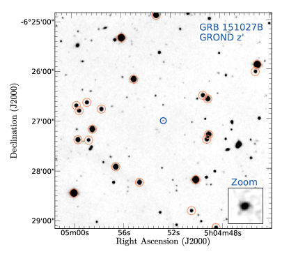
Figure 1: Finding chart of the afterglow of GRB 151027B based on a GROND $z^{\prime}$-band image, with secondary standard stars of Tab. 3 encircled. North is up, and East to the left.

Table 1: GROND observations; all in the AB system, not corrected for Galactic foreground extinction corresponding to $E(B-V)=0.18$ mag ($A_{V}=0.55$ mag) (Schlafly & Finkbeiner, 2011).

Time after $T_{0}$	$g^{\prime}$	$r^{\prime}$	$i^{\prime}$	$z^{\prime}$	$J$	$H$	$K_{\rm s}$
(s)	(mag)	(mag)	(mag)	(mag)	(mag)	(mag)	(mag)
$28830\pm 903$	$22.16\pm 0.23$	$20.41\pm 0.05$	$19.78\pm 0.04$	$19.58\pm 0.04$	$19.47\pm 0.09$	$18.96\pm 0.08$	$19.09\pm 0.16$
$30948\pm 1125$	$22.17\pm 0.26$	$20.59\pm 0.07$	$20.02\pm 0.06$	$19.66\pm 0.05$	$19.48\pm 0.10$	$19.19\pm 0.10$	$19.10\pm 0.20$
$33291\pm 1129$	$22.69\pm 0.24$	$20.62\pm 0.04$	$20.00\pm 0.04$	$19.67\pm 0.04$	$19.52\pm 0.07$	$19.17\pm 0.08$	$19.10\pm 0.14$
$35634\pm 1130$	$22.45\pm 0.16$	$20.64\pm 0.04$	$20.08\pm 0.04$	$19.77\pm 0.04$	$19.54\pm 0.07$	$19.39\pm 0.08$	$19.24\pm 0.14$
$112431\pm 6317$	$>23.6$	$22.05\pm 0.07$	$21.53\pm 0.07$	$21.18\pm 0.06$	$21.10\pm 0.15$	$20.73\pm 0.16$	$20.36\pm 0.24$
$202273\pm 1606$	$>24.0$	$22.57\pm 0.09$	$22.09\pm 0.09$	$21.85\pm 0.08$	$21.80\pm 0.25$	$21.53\pm 0.29$	$>20.9$
$804300\pm 6436$	$>25.8$	$24.75\pm 0.16$	$24.33\pm 0.21$	$23.87\pm 0.23$	$>22.3$	$>21.9$	$>21.5$
$\!\!1838665\pm 3570$	$>25.5$	$>25.7$	$>24.9$	$>24.7$	$>22.4$	$>22.0$	$>21.4$

2.2 GROND observations

Observations with GROND (Greiner et al., 2008) started on 2015 October 28 at 06:26 UT, about 8 hr after the trigger, at a Moon distance of only 37^∘. Simultaneous imaging in $g^{\prime}r^{\prime}i^{\prime}z^{\prime}JHK_{\rm s}$ continued for several further epochs (see the observation log in Tab. 1) until 2015 November 18, when the afterglow could not be detected anymore. During the night of November 5/6, a field with SDSS coverage (RA(2000.0)=03h 45m, Decl.(2000.0)=-06^∘15^′) was observed immediately after the GRB field under photometric conditions.

Table 2: ATCA observing details

Date & Start-Time	On source	Time after GRB	Telescope	5.5 GHz flux	9 GHz flux
	exposure (hr)	(days)a)	configuration	$\mu$Jyb)	$\mu$Jyb)
2015-10-30 12:56	3.3	2.76$\pm$0.16	6A	$<$18	67$\pm$10
2015-11-02 12:00	3.2	5.74$\pm$0.19	6A	73$\pm$10	98$\pm$11
2015-11-11 15:36	5.8	14.70$\pm$0.19	6A	76$\pm$7	$<$15
2015-11-14 11:31	3.3	17.69$\pm$0.16	6A	$<$26.0	100$\pm$10
2015-11-16 12:00	6.7	19.72$\pm$0.17	1.5A	$<$13.4	$<$15.4
2015-12-02 09:36	8.4	35.67$\pm$0.21	1.5A	60$\pm$11	36$\pm$11
2015-12-11 10:05	2.5	44.54$\pm$0.06	750C	71$\pm$12	$<$22
2016-01-22 06:30	5.7	86.48$\pm$0.16	EW352	$<$24	$<$28

^a) The “error” denotes the time span over which the exposure was spread to cover the $u-v$ plane. ^b) Upper limits are given at the 2$\sigma$ level.

GROND data have been reduced in the standard manner (Krühler et al., 2008) using pyraf/IRAF (Tody, 1993; Küpcü Yoldaş et al., 2008). The optical/NIR imaging was calibrated against the primary SDSS standard star network, or catalogued magnitudes of field stars from the SDSS in the case of $g^{\prime}r^{\prime}i^{\prime}z^{\prime}$ observations, or the 2MASS catalog for $JHK_{\rm s}$ imaging. This results in typical absolute accuracies of $\pm$0.03 mag in $g^{\prime}r^{\prime}i^{\prime}z^{\prime}$ and $\pm$0.05 mag in $JHK_{\rm s}$. Comparison stars covered by the finding chart of GRB 151027B (Fig. 1) are given in Tab. 3.

Despite its high redshift, the afterglow was detected in all seven bands (Tab. 1) at a common position of RA(2000.0), Dec(2000.0) = 76$\aas@@fstack{\circ}$21955, -6$\aas@@fstack{\circ}$45029, or 05:04:52.69 –06:27:01.1, with a 1$\sigma$ error of $\pm$0$\aas@@fstack{\prime\prime}$25. This is fully consistent with both, the UVOT-corrected Swift/XRT position (Osborne et al., 2015) as well as the NOT-derived position (Malesani et al., 2015).

2.3 ATCA observations

We observed the field of GRB 151027B under program C2955 (PI: Greiner) simultaneously at 5.5 and 9 GHz with the Australia Telescope Compact Array (ATCA), beginning at October 30.54 UT for 3.3 hr; the corresponding detection at 9 GHz has been reported earlier (Greiner et al., 2015b). Over the following three months, we observed the GRB 151027B position at another 7 epochs. A summary of the observing log, including the telescope configuration, is given in Tab. 2. The observations were mostly performed with the CFB 1M-0.5K mode, providing 2048 channels per 2048 MHz continuum intermediate frequency (IF; 1 MHz resolution) and 2048 channels per 1 MHz zoom band (0.5 kHz resolution). Data analysis was done using the standard software package MIRIAD (Sault et al., 1995), applying appropriate bandpass, phase and flux calibrations. The quasar 0458-020 was used as phase and 1934-638 as flux calibrator. Multifrequency synthesis images were constructed using robust weighting (robust=0) and the full bandwidth between its flagged edges. The noise was determined by estimating the root-mean-square (rms) in emission-free parts of the cleaned map.

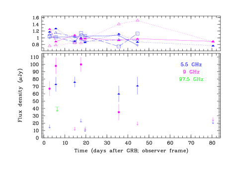
Figure 2: Radio light curve of the afterglow of GRB 151027B at 5.5 and 9 GHz, with the ALMA 97.5 GHz 2$\sigma$ upper limit overplotted (lower panel). The upper panel shows the measured fluxes of selected brighter (130-500 $\mu$Jy) sources. While their nature or intrinsic variability is not known, their $<$20% flux variation demonstrates that the strong fluctuations seen for the GRB 151027B afterglow (which would correspond to an amplitude between 0.2 and 2 in this graph) is not an instrumental artifact.

Given the largely varying flux levels between different observations and also large flux differences between the two frequencies, we note that the signal-to-noise ratio in most detections is so high that it is unlikely our measurements are wrong. We employed two further tests: 1) for the November 14 observation, we made separate images for the top and bottom of the 9 GHz band, resulting in flux measurements of 96 $\mu$Jy (8-9 GHz) and 106 $\mu$Jy (9-10 GHz), thus providing an internally consistent result; 2) we checked for other sources in the field for evidence of such variation, but did not find any (see Fig. 2).

2.4 ALMA observations

ALMA observations were triggered under proposal-ID 2015.1.01558.T (PI: S. Schulze). A band 7 (343.495 GHz) observation was performed starting on 2015 November 2, 05:22 UT under a precipitable water vapour (PWV) of 0.71 mm, and a band 3 (97.495 GHz) observation started on 2015 November 4 at 07:45 UT under a PWV=0.31 mm. The data analysis was performed using the standard ALMA data analysis package CASA (McMullin et al., 2007; Petry et al., 2012), following the default calibration path also used in ALMA Quality Assurance. The final images are shown in Fig. 3.

Within the GROND error circle of 0$\aas@@fstack{\prime\prime}$25, in band 3, we find a peak with a flux of 0.0619 mJy which given the rms noise of 0.0210 mJy corresponds to nearly 3$\sigma$. However, the area of the error circle contains 1914 spatial resolution pixels, so we expect 1914 pixels $\times$ 0.0016 = 3 pixels to be above a 3$\sigma$ flux level. Thus, the presence of the source-like point in the error circle is compatible with a random occurrence, likely thermal noise. In fact, there are similar peaks outside the error circle.

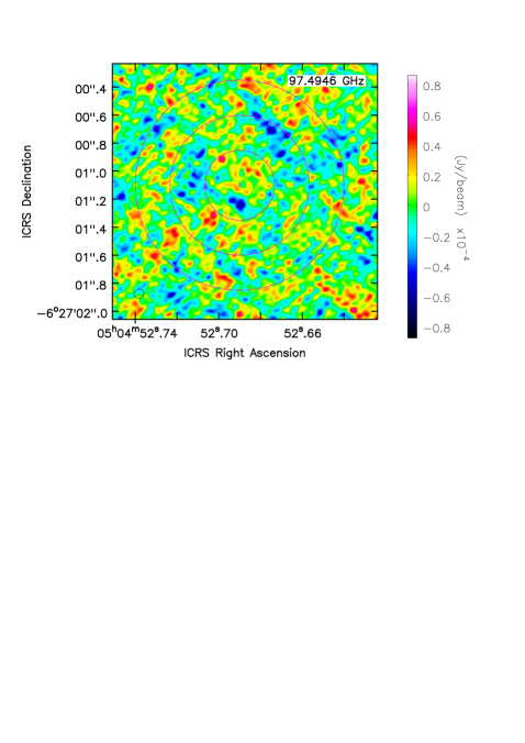
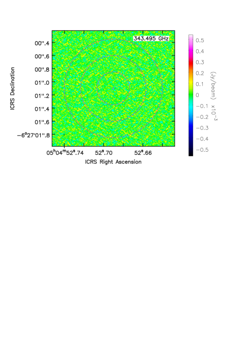
Figure 3: ALMA images of the GRB 151027B location at band 3 (97.5 GHz; left) and band 7 (343.5 GHz; right), in the International Celestial Reference System (ICRS). The concentric circles around our best-fit GROND position are the 1$\sigma$, 2$\sigma$ and 3$\sigma$ error circles. The contour in the lower left of each figure gives the size of the synthesized beam of the observation. It is due to the smaller beam size that the band 7 image visually looks smoother than that of band 3; the rms-noise is actually worse, as given in the text.

In band 7, we find a peak within the error circle of 0.177 mJy which given the rms noise of 0.0496 mJy corresponds to 3.5$\sigma$. However, the area of the error circle contains 7793 spatial resolution pixels, so we expect 7793 pixels $\times$ 0.0002 = 1.6 pixels to be above a 3.5$\sigma$ flux level.

Summarizing, no source is detected in either observation, with 2$\sigma$ upper limits of 42 $\mu$Jy in band 3 (97.495 GHz, integrated over a bandwidth of 7 GHz; taking into account that only about 87% of each of the four spectral windows was used; edge channels are not good) at 7.378 days after the GRB, and 100 $\mu$Jy in band 7 (343.495 GHz, also with a bandwidth of 7 GHz) at 5.279 days after the GRB. These values include the primary beam correction (though this is $>$0.99 due to being close to the center of the field of view).

3 Results

Here, we will analyze our data in the context of the GRB fireball model (Meszaros & Rees, 1997; Granot & Sari, 2002). Throughout this paper, we use the definition $F_{\nu}\propto t^{-\alpha}\nu^{-\beta}$ where $\alpha$ is the temporal decay index, and $\beta$ is the spectral slope.

3.1 Radio scintillation

The large-amplitude radio variability observed in this GRB is very unusual. In the context of the canonical fireball scenario one would expect a smoothly varying afterglow, perhaps with a rapid rise and decay due to reverse shock emission, none of which is akin to our data. Moreover, we observe large variations between the simultaneously covered 5.5 and 9 GHz bands, i.e. the inferred spectral slope changes between $<-2.3$ and $>2.9$ within days, while temporal slopes in the range $<-15$ and $>9$ over $2-3$ days are implied. We are not aware of any physical process(es) in GRB jets or shocks capable of producing emission with such properties, and thus consider the afterglow radio emission to be strongly influenced by scintillation.

Interstellar scintillation effects have been observed in GRB radio light curves, and used to obtain indirect measures of the source size (for a recent review, see Granot & van der Horst, 2014). This method relies on the fact that propagation effects in the interstellar medium cause modulations of the flux of a compact source, while a source larger than a certain angular size will not vary (Rickett, 1990). In the case of GRBs, the source is the evolving shock front of the jet, which is very compact at first but expands over time. This can result in strong modulations at early times, which get quenched at later times (Frail et al., 1997; Goodman, 1997; Frail et al., 2000). These variations can be found between observations on different days, but intraday variability has also been observed in GRBs (e.g., Chandra et al., 2008; van der Horst et al., 2014). The typical procedure for relating the source size to the scintillation effects is to estimate the scintillation strength and timescale using the methods of Walker (1998) combined with the NE2001 model of the free electrons in our galaxy (Cordes & Lazio, 2002). In the strong scattering regime, there are two possible types of scintillation: refractive and diffractive. In both cases the modulation strength depends on the source size compared to the angular scale for scintillation, which ranges from a few to a few tens of micro-arcseconds. Diffractive scintillation gives stronger flux modulations than refractive scintillation, but the angular scale for diffractive scintillation is smaller than that for refractive scintillation. Furthermore, the former is a narrow-band phenomenon while the latter is broad-band, but they could both be at play in GRB afterglow observations.

The redshift of GRB 151027B is 4.063, which means that 1 arcsecond on the sky corresponds to a distance of 7.05 kpc, so 1 micro-arcsecond corresponds to $2.2\times 10^{16}$ cm. A size of $10^{16}-10^{17}$ cm is typical for the jet size, so strong scintillation effects are expected for this GRB, also because the high redshift of the GRB means that 40 days in the observer frame corresponds to 8 days in the source rest frame. The scintillation timescale of several hours to days that we observe for GRB 151027B is plausible, but the observed modulation seems to be too large to accommodate within this framework. The maximum modulation index for diffractive scintillation is 1, i.e. the flux can increase or decrease by a factor of 2 due to scintillation, and the modulation index for refractive scintillation is always smaller than 1. Both of those are significantly smaller than the jumps in flux that we have observed for GRB 151027B, which are more than a factor of 5 between some observations (at the $2\sigma$ level). For instance, at 9 GHz the flux fluctuates from $<15\mu$Jy at 14.7 days, to $100\pm 10\mu$Jy at 17.7 days, and then $<15\mu$Jy at 19.7 days; flux changes of more than a factor of 5, both up and down.

Given that these strong flux modulations can not be explained by physical processes in the source itself, scintillation does seem to be the most natural way to explain the observations, as has been done for other GRBs with radio flux modulations. However, in this particular case, we seemingly have to deviate from the typical methodology applied in the modeling of scintillation effects on GRB radio light curves due to the very large and fast modulations. One of the underlying assumptions of the usual methodology is that the scattering happens at one location, the scattering screen, which resides at a typical distance (usually 1 kpc from the observer). However, many studies of interstellar scintillation with pulsars and active galactic nuclei have shown that the distance of the scattering screen is quite uncertain. Varying this distance can have strong effects on both the modulation strength and timescale. For example, some quasars have shown extreme intraday variability, indicating that their scattering screen is significantly closer than what is usually assumed (Dennett-Thorpe & de Bruyn, 2002; Bignall et al., 2006; Macquart & de Bruyn, 2007; de Bruyn & Macquart, 2015). Furthermore, extragalactic sources may be shining through multiple scattering screens inside our galaxy, complicating the scintillation behavior even further. Every scattering screen will impose its own modulation strength and timescale, possibly leading to enhanced and complex scintillation behaviour.

The bottom line is that the observed fluctuations in GRB 151027B can be explained by scintillation, but the large modulation amplitude and rapid variations suggests that the scattering screen is at a smaller distance, that there are multiple screens, or a combination of the two. It will require many more detailed studies of various radio sources, including GRB afterglows, to fully probe the scintillation behavior of the interstellar medium in our local environment.

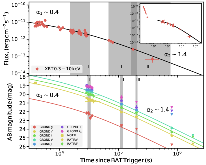
Figure 4: Light curve of the afterglow of GRB 151027B at X-rays as observed with Swift/XRT (top), and in the optical/near-infrared as observed with GROND (no extinction-correction applied), complemented with two measurements by NOT and RATIR (Malesani et al., 2015; Watson et al., 2015). Error bars are plotted, but mostly smaller than the symbol size. The vertical grey bands mark the time intervals for which the spectral energy distributions have been established (see text for more details and Fig. 5).

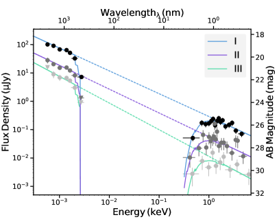
Figure 5: Observer-frame optical/near-infrared to X-ray spectral energy distribution of the afterglow of GRB 151027B at the three epochs marked in Fig. 4 with the grey shading. Error bars are plotted, but mostly smaller than the symbol size.

3.2 Constraints on the fireball model

Both the X-ray and the optical light-curves can be modeled with a smoothly broken power-law (Fig. 4) with $\alpha_{1}=0.44\pm 0.19$, $\alpha_{2}=1.44\pm 0.14$ and $t_{b}\sim 22.5$ ks, consistent with the magnitudes observed by NOT and RATIR (Malesani et al., 2015; Watson et al., 2015). These temporal slopes were used to rescale an XRT spectrum from data taken between $T_{0}+15$ ks and $T_{0}+32$ ks to the stacked GROND data taken between $T_{0}+32$ ks and $T_{0}+34$ ks (both these intervals are shaded in grey in Fig. 4). The resulting broadband spectral energy distribution (SED) is best fit with a single power-law of slope $\beta=0.81\pm 0.01$, with a negligible amount of dust ($A_{V}=0.01\pm 0.01$ mag), independent of the extinction model (see Bolmer et al. 2018 for more details on the extinction determination, where a broken power-law model has been preferred in order to derive a conservative extinction value). In these fits, the $g^{\prime}$$r^{\prime}$ filters were ignored owing to additional uncertainty from absorption from the Ly$\alpha$ forest. The spectral slope in the X-ray to optical/near-infrared does not change with time within errors ($\beta_{1}=0.81\pm 0.01$, $\beta_{2}=0.83\pm 0.03$ and $\beta_{3}=0.89\pm 0.07$) as evidenced by the other broadband SEDs at later times (see Fig. 5), nor do the data require a spectral break at later times. The above post-break parameters are fully consistent (within 2$\sigma$) with an afterglow with an electron powerlaw distribution with $p=2.62\pm 0.02$, evolving via slow cooling into an ISM environment where the cooling break is above the Swift/XRT upper energy boundary: measured $\alpha_{2}=1.44\pm 0.14$ vs. predicted $\alpha_{2}=1.22\pm 0.02$. A cooling break below the GROND bands would imply $p=1.62\pm 0.02$ and $\alpha_{2}=0.72$, inconsistent with our observed light curve. In the preferred scenario, the cooling break $\nu_{c}$ would move to lower frequencies proportional to $t^{-1/2}$. Since we also do not see any signature of a spectral break in the X-ray band up to 2$\times$10⁵ s after the GRB, after back-extrapolation this implies that $\nu_{c}$ (31 ks) $>$ 20 keV. We finally note that the pre-break phase is consistent with the plateaus seen in many Swift-detected GRBs (e.g., Dainotti et al., 2017, and references therein), with the optical data (primarily the NOT data) fitting the picture as well as evidenced by being in the same synchrotron spectral regime.

The remaining question then is the relative ordering of the peak frequency $\nu_{m}$ and the self-absorption frequency $\nu_{sa}$. Given the multiple radio detections with ATCA implies that the self-absorption frequency should be below 5 GHz already at 2.8 days after the GRB in order for the scintillation amplitude not to exceed a factor of 10. The ALMA limits then require $\nu_{m}$ to be above the self-absorption frequency. Considering the canonical decrease of $\nu_{m}$ according to $t^{-3/2}$, our following two observational constraints fix the value of $\nu_{m}(t)$ to better than 20%: (i) at the time of the first GROND observation, $\nu_{m}$(31 ks)$<1.3\times 10^{14}$ Hz; (ii) the ALMA band 7 limit together with the interpolated optical/near-infrared fluxes at this epoch imply $\nu_{m}$(5.279 d)$>1.8\times 10^{12}$ Hz. Back-extrapolating the latter limit to the first GROND observation (by a factor of (31 ks/456.1 ks)^-3/2 = 56.4) implies an inferred $\nu_{m}$(31 ks)$=(1.15\pm 0.15)\times 10^{14}$ Hz.

With these observational constraints it is possible to determine the fireball parameters, as follows: We observe the following set of relations, all at 31 ks after the GRB:

$$\nu_{m}=(1.15\pm 0.15)\times 10^{14}\,{\rm Hz}$$

$$F_{\nu}(\nu_{m})=(100\pm 10)\,\mu{\rm Jy}$$

$$\nu_{c}>4.8\times 10^{18}\,{\rm Hz}\,\,(=20\,{\rm keV})$$

$$F_{\nu}(\nu_{c})<0.07\,\mu{\rm Jy}$$

Within the canonical fireball scenario (Granot & Sari, 2002) in the slow cooling case with the ordering $\nu_{sa}<\nu_{m}<\nu_{c}$ and ISM density profile, the self-absorption frequency remains constant, and being always below 100 MHz, i.e. below our observed frequencies, for all the allowed parameter range (see below), it does not provide any further constraint.

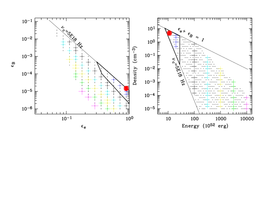
Figure 6: Constraints on the fireball parameters for the afterglow of GRB 151027B. Small black dots delineate the allowed phase space by the four constraints at 31 ks, and colored crosses visualize different possible solutions for seven different values of the kinetic energy. The solution with the lowest kinetic energy is marked with the red-filled octagon: $E_{\rm kin}=11.2\times 10^{52}$ erg, external density $n=5$ cm^-3, $\epsilon_{e}=0.9$ and $\epsilon_{B}=1.5\times 10^{-5}$. The thick-lined triangles enclose the allowed parameter range, if $E_{\rm kin}<5\times E_{\rm\gamma,iso}$.

These constraints on the observed frequencies and fluxes lead to bounds on the fireball parameters as visualized in Fig. 6. While the observations do not uniquely constrain all parameters we can use an efficiency argument to derive a likely parameter range. In the standard picture, a fraction $\epsilon_{\gamma}$ of the explosion energy is radiated in the prompt radiation (observable as $E_{\rm\gamma,iso}$), and the remaining fraction ending up as kinetic energy $E_{\rm kin}$ of the swept up ambient gas. Early observations suggested nearly equipartition between these two channels, though later considerations including proper error estimates suggest $\epsilon_{\gamma}$ in the range of $\sim 0.1-0.5$ (Granot et al., 2006). Assuming $\epsilon_{\gamma}=0.2$ and using $E_{\rm\gamma,iso}$ (15–10000 keV) = $(5\pm 1)\times 10^{52}$ erg (based on a best-fit cut-off powerlaw fit of the Swift/BAT data provided at http://gcn.gsfc.nasa.gov/notices_s/661869/BA/ giving an energy fluence of (14.7$\pm$2.6) $\times 10^{-7}$ erg cm^-2), the GRB 151027B fireball parameters are constrained as follows: external density $n=0.03-5$ cm^-3, $\epsilon_{e}=0.3-1.0$ and $\epsilon_{B}=4\times 10^{-4}-2\times 10^{-6}$ (see Fig. 6). We note that our derived $\epsilon_{e}$ is higher than the majority of published afterglows, though still in the allowed range.

For the solution with the lowest kinetic energy, $E_{\rm kin}=11.2\times 10^{52}$ erg (remaining parameters see caption of Fig. 6), we then compute the X-ray, optical I-band and 7 GHz radio (as average between 5.5 and 9 GHz) light curves. These are shown in Fig. 7. Note that the model was derived without using constraints from the radio bands, so it is interesting that the ’predicted’ radio light curve of Fig. 7 corresponds roughly to the mean of the radio detections and upper limits. This implies that the scintillation interpretation of the measured radio fluxes is reasonable. Thus, the observed scintillation corresponds to about a factor $\pm$3 variation in either direction, but is not a one-way excursion.

4 Conclusions

Our data set of the GRB 151027B afterglow can be explained with the simplest version of the standard fireball scenario, displaying a single synchrotron spectrum evolving according to standard dynamics.

We find that the blast wave moves into a constant-density environment, in the slow cooling regime. While we do not see the characteristic movement of the cooling frequency in or through the X-ray band, the constancy of the peak flux over the full observing epoch as evidenced by our data requires a constant density profile. The derived fireball parameters are all within the range expected and discussed in the literature. For the smallest allowed kinetic energy, $\epsilon_{e}$ is pushed towards the upper limit of 1.

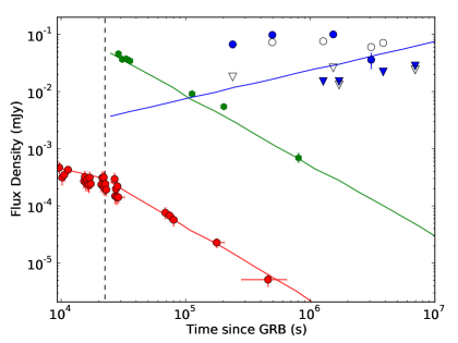
Figure 7: Model light curves for the afterglow of GRB 151027B at X-rays (red), optical (green, extinction-corrected) and radio (blue; open/filled symbols are 5.5/9 GHz, respectively; circles=detection, triangles=upper limits) for the lowest-$E_{\rm kin}$ parameter set. Data are drawn with error bars, but those are mostly smaller than the symbol size. The vertical line denotes the break time of 22.5 ks (see sect. 3.2). Radio data have not been used in deriving the model, so the blue curve is actually a ‘predicted’ light curve. The fact that it matches the mean between the radio measurements and upper limits demonstrates that the model is reasonably good, and that the scintillation interpretation for the radio measurements is reasonable.

After GRBs 000131, 050904, 090423, 111008A, 120521C, 130606A, 140304A, 140311A, 140515A the afterglow of GRB 151027B is the tenth above a redshift of 4 which is detected in the radio band (see the summary table http://www.mpe.mpg.de/^∼jcg/grbgen.html). Its peak spectral radio luminosity (2$\times$10³¹ erg/s/Hz) is among the top quarter of radio afterglows (Chandra & Frail, 2012), but certainly not exceptional. However, the large-amplitude and rapid flux fluctuations up to 9 GHz are exceptional, and imply that scintillation plays a major role, even at 45 days (9 days rest-frame) post-burst.

We finally mention that the ALMA flux limits are close to the prediction of our model, so we cannot completely rule out that the 3.5$\sigma$ blob in the band 7 image is not, indeed, the afterglow.

With the above caveats it is worth noting that this is one of the few afterglows of long-duration GRBs for which the simplest version of the afterglow scenario describes a rather extensive multi-epoch and multi-frequency data set. In many cases, more data also meant a need for a more complicated afterglow scenario. This is independent of the publication bias that afterglows with ’exciting’ irregular behaviour (like GRBs 071031 – Krühler et al. 2009, 080129 – Greiner et al. 2009, 081029 – Nardini et al. 2011, 100621A – Greiner et al. 2013, 100814A – Nardini et al. 2014, 111209A – Greiner et al. 2015a; Kann et al. 2018) get more easily published than standard GRB afterglows. It remains to be investigated whether or not some of the standard afterglows can be fitted with the next-simplest version of afterglow models. The hydrodynamical simulations including the incorporation of the off-axis angle view (van Eerten, 2015) represent one way, analytical jet spreading models another.

While there is a wealth of published papers dealing with the (fireball) modelling of individual GRB afterglows, the vast majority only allows consistency checks, since the data are not sufficient to derive all five (plus redshift) model parameters. The three historical exceptions for which all parameters could be determined are GRBs 980703 (Frail et al., 2003), 000926 (Harrison et al., 2001) and 090323 (Cenko et al., 2011). More recently, our group managed to add another 4 GRBs to this sample (100418A, 110715A, 121024A, 130418A – (Varela, 2017); for GRB 121024A see Varela et al. (2016) for details. This small sample, out of a total of $>$700 known X-ray/optical afterglows, shows the challenge of testing the afterglow model(s). And even those seven GRB afterglows are not uniquely described by a single set of parameters or the simplest fireball version: one GRB is equally well described by either wind or ISM density profile, two other GRBs show substantial flaring activity implying additional energy injection, and another two GRBs show strong evidence for an inverse Compton component. There are indications in this sample for a preference of a wind-like GRB environment, contrary to the results of many early analyses. However, this topic as well as other afterglow-related issues like a reliable distribution of microphysical parameters, require a substantially larger sample size.

From an observer point of view, it is not obvious how to best reach a larger sample size, i.e. how a guaranteed-success strategy would look like. Radio observations are only meaningful at late times when scintillation has ceased, but then the X-ray and optical/NIR instrumentation typically is not sensitive enough to detect the afterglow anymore. Yet, radio observations provide crucial constraints for the afterglow modelling. Alternatively, dedicated multi-band, multi-epoch ALMA monitoring seems promising for two reasons: Firstly, it is sensitive enough to cover a larger time interval of the afterglow emission (say 2-3 weeks). Secondly, the $\nu_{m}$-crossing is faster than that of $\nu_{c}$, allowing (in combination with the decay slope) a potentially better distinction between wind and ISM environment. While rapid (within a day) target-of-opportunity (ToO) observations are finally allowed with ALMA, the general acceptance level of GRB-related ToO-proposals is going down after more than a decade of Swift-driven afterglow studies, and the need for getting proposals accepted at several observatories during the same semester does not make things easier (see e.g. Middleton et al. 2017 for a description of the problem and suggested solutions). Instead of attempting full multi-wavelength coverage over a long time-interval, a graded approach with dense X-ray/optical/sub-mm coverage during the first days and sub-mm/radio at late stages might be the better approach. This is particularly motivated by the potential of trans-relativistic dynamical models and models including jet dynamics, that improve upon earlier closure relations. The number of open questions and the impact which a proper knowledge of the GRB afterglow emission process would have on a variety of other astrophysical areas certainly justifies a concerted approach.

Facilities: Max Planck:2.2m (GROND), ATCA, ALMA, Swift

Table 3: Secondary standard stars used to calibrate the optical/NIR afterglow measurements. The $g^{\prime}$$r^{\prime}$$i^{\prime}$$z^{\prime}$ magnitudes are in the AB system, $JHK_{\rm s}$ in Vega.

RA/Decl. (deg)	RA/Decl. (hms)	$g^{\prime}$	$r^{\prime}$	$i^{\prime}$	$z^{\prime}$	$J$	$H$	$K_{\rm s}$
(2000.0)	(2000.0)	(mag)	(mag)	(mag)	(mag)	(mag)	(mag)	(mag)
76.22154 -6.41494	05:04:53.17 -06:24:53.8	16.838$\pm$0.001	15.947$\pm$0.001	15.664$\pm$0.001	15.440$\pm$0.001	14.437$\pm$0.002	14.000$\pm$0.002	13.860$\pm$0.009
76.23341 -6.42239	05:04:56.02 -06:25:20.6	15.289$\pm$0.001	14.961$\pm$0.001	14.475$\pm$0.001	14.325$\pm$0.001	13.375$\pm$0.001	13.022$\pm$0.002	12.860$\pm$0.004
76.18746 -6.43186	05:04:44.99 -06:25:54.7	15.155$\pm$0.001	14.914$\pm$0.001	14.441$\pm$0.001	14.308$\pm$0.001	13.374$\pm$0.001	13.023$\pm$0.002	13.047$\pm$0.004
76.18821 -6.43417	05:04:45.17 -06:26:03.0	18.943$\pm$0.009	18.278$\pm$0.004	18.046$\pm$0.005	17.858$\pm$0.005	16.910$\pm$0.020	16.439$\pm$0.027	16.338$\pm$0.089
76.22938 -6.43628	05:04:55.05 -06:26:10.6	16.412$\pm$0.001	15.793$\pm$0.001	15.512$\pm$0.001	15.323$\pm$0.001	14.381$\pm$0.002	13.936$\pm$0.002	13.853$\pm$0.009
76.20600 -6.44189	05:04:49.44 -06:26:30.8	19.557$\pm$0.014	17.987$\pm$0.003	17.294$\pm$0.003	16.894$\pm$0.002	15.656$\pm$0.005	14.906$\pm$0.007	14.848$\pm$0.023
76.20441 -6.44311	05:04:49.06 -06:26:35.2	18.429$\pm$0.005	16.989$\pm$0.001	16.419$\pm$0.001	16.063$\pm$0.001	14.871$\pm$0.004	14.159$\pm$0.004	14.115$\pm$0.012
76.24538 -6.44383	05:04:58.89 -06:26:37.8	18.927$\pm$0.007	17.926$\pm$0.003	17.539$\pm$0.003	17.282$\pm$0.003	16.177$\pm$0.007	15.552$\pm$0.009	15.483$\pm$0.037
76.24888 -6.44475	05:04:59.73 -06:26:41.1	18.823$\pm$0.007	17.953$\pm$0.003	17.592$\pm$0.003	17.350$\pm$0.003	16.287$\pm$0.009	15.775$\pm$0.012	15.698$\pm$0.046
76.24046 -6.44611	05:04:57.71 -06:26:46.0	18.042$\pm$0.003	17.457$\pm$0.002	17.242$\pm$0.002	17.068$\pm$0.002	16.179$\pm$0.007	15.785$\pm$0.012	15.733$\pm$0.046
76.24809 -6.44664	05:04:59.54 -06:26:47.9	18.253$\pm$0.004	17.550$\pm$0.002	17.278$\pm$0.002	17.084$\pm$0.003	16.097$\pm$0.007	15.634$\pm$0.011	15.586$\pm$0.039
76.24358 -6.45283	05:04:58.46 -06:27:10.2	16.975$\pm$0.001	16.058$\pm$0.001	15.684$\pm$0.001	15.422$\pm$0.001	14.353$\pm$0.002	13.896$\pm$0.002	13.711$\pm$0.007
76.20421 -6.45503	05:04:49.01 -06:27:18.1	16.637$\pm$0.001	16.080$\pm$0.001	15.909$\pm$0.001	15.760$\pm$0.001	14.888$\pm$0.002	14.595$\pm$0.005	14.589$\pm$0.014
76.24854 -6.45628	05:04:59.65 -06:27:22.6	17.206$\pm$0.002	16.637$\pm$0.001	16.419$\pm$0.001	16.259$\pm$0.001	15.334$\pm$0.004	15.057$\pm$0.007	14.938$\pm$0.018
76.24492 -6.45639	05:04:58.78 -06:27:23.0	19.816$\pm$0.017	18.618$\pm$0.005	18.125$\pm$0.005	17.828$\pm$0.005	16.660$\pm$0.014	16.090$\pm$0.018	–
76.20492 -6.45661	05:04:49.18 -06:27:23.8	17.422$\pm$0.002	16.985$\pm$0.001	16.840$\pm$0.002	16.710$\pm$0.002	15.832$\pm$0.007	15.538$\pm$0.011	15.668$\pm$0.039
76.23579 -6.46542	05:04:56.59 -06:27:55.5	17.697$\pm$0.002	16.485$\pm$0.001	16.035$\pm$0.001	15.720$\pm$0.001	14.555$\pm$0.002	13.993$\pm$0.002	13.858$\pm$0.007
76.20871 -6.46989	05:04:50.09 -06:28:11.6	17.155$\pm$0.002	15.646$\pm$0.001	14.865$\pm$0.001	14.477$\pm$0.001	13.231$\pm$0.001	12.624$\pm$0.001	12.455$\pm$0.002
76.22787 -6.47075	05:04:54.69 -06:28:14.7	19.456$\pm$0.014	17.722$\pm$0.002	16.879$\pm$0.002	16.392$\pm$0.001	15.037$\pm$0.004	14.370$\pm$0.004	14.142$\pm$0.009
76.25004 -6.47411	05:05:00.01 -06:28:26.8	14.953$\pm$0.001	14.683$\pm$0.001	14.181$\pm$0.001	13.959$\pm$0.001	12.881$\pm$0.001	12.503$\pm$0.001	12.362$\pm$0.002
76.21046 -6.48039	05:04:50.51 -06:28:49.4	20.958$\pm$0.052	19.300$\pm$0.010	18.445$\pm$0.007	17.950$\pm$0.005	16.676$\pm$0.012	15.973$\pm$0.014	15.843$\pm$0.043
76.20200 -6.48617	05:04:48.48 -06:29:10.2	20.425$\pm$0.035	18.816$\pm$0.007	17.941$\pm$0.005	17.449$\pm$0.004	16.118$\pm$0.007	15.430$\pm$0.009	15.310$\pm$0.027

References

- Barthelmy et al. (2005) Barthelmy S.D., Barbier L.M., Cummings J.R., et al. 2005, Space Sci. Rev. 120, 143
- Bignall et al. (2006) Bignall, H. E., Macquart, J.-P., Jauncey, D. L., et al. 2006, ApJ 652, 1050
- Bolmer et al. (2018) Bolmer J., Greiner J., Krühler T., et al. 2018, A&A 609, A62
- Breeveld et al. (2015) Breeveld A.A, Ukwatta T.N., 2015, GCN Circ. #18517
- Buckley et al. (2015) Buckley D., Potter S., Kniazev A., et al. 2015, GCN Circ. #18511
- Burrows et al. (2005) Burrows D.N., Hill J.E., Nousek J.A. et al. 2005, SSR 120, 165
- Cenko et al. (2010) Cenko S.B., Frail D.A., Harrison F.A., et al. 2010, ApJ 711, 641
- Cenko et al. (2011) Cenko S.B., Frail D.A., Harrison F.A., et al. 2011, ApJ 732, 29
- Chandra et al. (2008) Chandra, P., Cenko, S.B., Frail, D.A., et al. 2008, ApJ 683, 924
- Chandra & Frail (2012) Chandra, P., Frail, D.A., 2012, ApJ ApJ 746, 156
- Cordes & Lazio (2002) Cordes, J.M., & Lazio, T.J.W. 2002, arXiv:astro-ph/0207156
- de Bruyn & Macquart (2015) de Bruyn, A.G., & Macquart, J.-P. 2015, A&A 574, A125
- Dainotti et al. (2017) Dainotti M.G., Hernandez X., Postnov S., et al. 2017, ApJ 848, 88
- Dennett-Thorpe & de Bruyn (2002) Dennett-Thorpe, J., & de Bruyn, A. G. 2002, Nature 415, 57
- Dichiara et al. (2015) Dichiara S., Kopac D., Guidorzi C., Kobayashi S., Gomboc A., 2015, GCN Circ. #18520
- Frail et al. (1997) Frail D.A., Kulkarni S.R., Nicastro L., Feroci M., Taylor G.B., 1997, Nature 389, 261
- Frail et al. (2000) Frail D.A., Waxman E., & Kulkarni S.R. 2000, ApJ 537, 191
- Frail et al. (2003) Frail D.A., Yost S.A., Berger E. et al. 2003, ApJ 590, 992
- Gehrels et al. (2004) Gehrels N., Chincarini G., Giommi P., et al. 2004, ApJ 621, 558
- Goodman (1997) Goodman, J. 1997, New A 2, 449
- Granot & Sari (2002) Granot J., Sari R., 2002, ApJ 568, 820
- Granot et al. (2006) Granot J., Königl A., Piran T., 2006, MN 370, 1946
- Granot & van der Horst (2014) Granot, J., & van der Horst, A. J. 2014, PASA 31, e008
- Greiner et al. (2008) Greiner J., Bornemann W., Clemens C., et al. 2008, PASP 120, 405
- Greiner et al. (2009) Greiner J., Krühler T., McBreen S., et al. 2009, ApJ 693, 1912
- Greiner et al. (2013) Greiner J., Krühler T., Nardini M. et al. 2013, A&A 560, A70
- Greiner et al. (2015a) Greiner J., Mazzali P.A., Kann D.A. et al. 2015, Nat. 523, 189
- Greiner et al. (2015b) Greiner J., Wieringa M., Wiseman P., 2015b, GCN Circ. #18548
- Harrison et al. (2001) Harrison F.A., Yost S.A., Sari R. et al. 2001, ApJ 559, 123
- Hjorth et al. (2003) Hjorth J., Sollermann J., Moller P. et al. 2003, Nature 423, 847
- Kann et al. (2018) Kann D.A., Schady P., Olivares E.F. et al. 2018, A&A (subm., arXiv:1706.00601)
- Krühler et al. (2008) Krühler T., Küpcü Yoldaş A., Greiner J., et al. 2008, ApJ 685, 376
- Krühler et al. (2009) Krühler T., Greiner J., McBreen S., et al. 2009, ApJ 697, 758
- Küpcü Yoldaş et al. (2008) Küpcü Yoldaş A., Krühler T., Greiner J., et al. 2008, AIP Conf. Proc., 1000, 227
- Laskar et al. (2014) Laskar T., Berger E., Tanvir N.R., et al. 2014, ApJ 781, 1
- Malesani et al. (2015) Malesani D., Tanvir N.R., Xu D., et al. 2015, GCN Circ. #18501
- Macquart & de Bruyn (2007) Macquart, J.-P., & de Bruyn, A. G. 2007, MNRAS, 380, L20
- McBreen et al. (2010) McBreen S., Krühler T., Rau A. et al. 2010, A&A 516, A71
- McMullin et al. (2007) McMullin J.P., Waters B., Schiebel D., Young W., Golap K., 2007, Astron. Data Analysis Software and Systems XVI (ASP Conf. Ser. 376), eds. R.A. Shaw, F. Hill, D.J. Bell, (San Francisco, CA; ASP), p. 127
- Meszaros & Rees (1997) Meszaros P., Rees M.J., 1997, ApJ 476, 232
- Middleton et al. (2017) Middleton M.J., Casella P., Ghandi P. et al. 2017, New Astron. Rev. 79, 26
- Nardini et al. (2011) Nardini M., Greiner J., Krühler T. et al. 2011, A&A 531, A39
- Nardini et al. (2014) Nardini M., Elliott J., Filgas R., et al. 2014, A&A 562, A29
- Osborne et al. (2015) Osborne J.P., Beardmore A.P., Evans P.A., Goad M.R., 2015, GCN Circ. #18504
- Panaitescu & Kumar (2002) Panaitescu A., Kumar P., 2002, ApJ 571, 779
- Petry et al. (2012) Petry D., CASA Development Team, 2012, Astron. Data Analysis Software and Systems XXI. Proc. of Conf. Paris, 6-10 Nov. 2011, eds. P. Ballester, D. Egret, N.P.F. Lorente, ASP Conf. Ser. 461, p. 849
- Rickett (1990) Rickett, B. J. 1990, ARA&A, 28, 561
- Sakamoto et al. (2015) Sakamoto T., Barthelmy S.D., Cummings J.R., et al. 2015, GCN Circ. #18514
- Sault et al. (1995) Sault R.J., Teuben P.J., Wright M.C.H., 1995, in ’Astronomical Data Analysis Software and Systems IV’, ed. R. Shaw et al., ASP Conf. Ser. 77, 433
- Schlafly & Finkbeiner (2011) Schlafly E.F., Finkbeiner D.P., 2011, ApJ 737, 103
- Stanek et al. (2003) Stanek K.Z., Matheson T., Garnavich P.M. et al. 2003, ApJ 591, L17
- Taylor et al. (1997) Taylor G.B., Frail D.A., Beasley A.J., Kulkarni S.R., 1997, Nature 389, 263
- Tody (1993) Tody D., 1993, in Astronomical Data Analysis Software and Systems II, ASP Conf. Ser. 52, ed. R.J. Hanisch, R.J.V. Brissenden, & J. Barnes, p. 173
- Ukwatta et al. (2015) Ukwatta T.N., Barthelmy S.D., Baumgartner W.H., 2015, GCN Circ. #18499
- van der Horst et al. (2014) van der Horst, A.J., Paragi, Z., de Bruyn, A.G., et al. 2014, MNRAS 444, 3151
- van Eerten (2015) van Eerten H., 2015, Jour. High-Energy Astrophys. 7, 23
- Varela et al. (2016) Varela K., van Eerten H., Greiner J. et al., 2016, A&A 589, A37
- Varela (2017) Varela K., 2017, Dissertation, TU Munich
- Walker (1998) Walker, M. A. 1998, MNRAS 294, 307
- Watson et al. (2015) Watson A.M., Butler N., Kutyrev A., et al. 2015, GCN Circ. #18512
- Xu et al. (2015) Xu D., Tanvir N.R., Malesani D., Fynbo J.P.U., 2015, GCN Circ. #18505
- Yoon et al. (2012) Yoon S.-C., Dierks A., Langer N., 2012, A&A 542, A113
- Yost et al. (2003) Yost S.A., Harrison F.A., Sari R., Frail D.A., 2003, ApJ 597, 459