Fast Piecewise-Affine Motion Estimation Without Segmentation

Abstract

Current algorithmic approaches for piecewise affine motion estimation are based on alternating motion segmentation and estimation. We propose a new method to estimate piecewise affine motion fields directly without intermediate segmentation. To this end, we reformulate the problem by imposing piecewise constancy of the parameter field, and derive a specific proximal splitting optimization scheme. A key component of our framework is an efficient one-dimensional piecewise-affine estimator for vector-valued signals. The first advantage of our approach over segmentation-based methods is its absence of initialization. The second advantage is its lower computational cost which is independent of the complexity of the motion field. In addition to these features, we demonstrate competitive accuracy with other piecewise-parametric methods on standard evaluation benchmarks. Our new regularization scheme also outperforms the more standard use of total variation and total generalized variation.

I Introduction

Two important prior models have been explored for motion estimation. The first one works with a dense representation of motion and imposes at each pixel a smoothness constraint [19] such as total variation (TV) [5, 56]. Its regularization terms are most often convex and well suited to a large collection of optimization techniques. The second type of prior model works with parametric representations of motion, which may be chosen to provide a satisfying match of 3D translations on the camera plane. In particular, piecewise-parametric estimation methods have yielded very accurate results [42, 37, 55]. Yet, in spite of these achievements, local smoothness priors are still preferred to piecewise-parametric ones in most motion estimation methods. The main reason is the difficulty of the optimization problem associated with the piecewise-parametric approach. In this work, we address this optimization issue.

The problem is usually formulated as the joint segmentation of the motion field and estimation of the parameters inside each region, following the seminal work of Mumford and Shah [25] for the image segmentation part. The interdependency of these two tasks translates into highly non-convex optimization. The existing solutions proceed iteratively by alternating an optimization step with respect to the image partition and an optimization step with respect ot the motion parameters. This alternance causes two main issues. Firstly, the resulting scheme is very sensitive to initialization and can only be used for refinement. Secondly, the computational cost is often prohibitive for practical applications. In particular, it depends on the number of regions, which should typically be very large to achieve high-accuracy.

In this paper, we propose a new method to estimate piecewise-affine motion fields. It eschews the explicit segmentation of motion, leading to the direct estimation of a piecewise-affine motion field. We revisit the standard formulation and impose a piecewise-constant regularization of the field of affine parameters. The key step of our algorithm is a specific proximal-splitting approach that yields a series of 1D piecewise-affine vectorial estimation problems. We propose an efficient solver that is based on dynamic programming and inspired by the works on segmentation described in [33, 35, 48].

Extensive experiments on the reference benchmarks MPI Sintel [7] and Kitti [16] show that our approach outperforms the standard TV and total generalized variation (TGV) regularizations, and that it is competitive with the best performing piecewise-parametric methods. Moreover, our optimization does not require any initialization of the motion field, and it is faster than other piecewise-parametric approaches. In particular, the computational time does not depend on the complexity of the motion field. Thus, our method combines the advantages of the piecewise-affine model with robustness and a low computational cost. It can be integrated as a regularizer in various motion estimation frameworks.

The outline of the paper is as follows: In Section II, we review related works and identify their limitations. In Section  III, we describe the model and optimization method that we propose. In Section IV, we evaluate the performance of our method on standard benchmarks.

II Related Works

Joint motion segmentation and parameter estimation has been formulated as an optimization problem of the form

$$J=\min_{\mathcal{R},{\bf w}}\leavevmode\nobreak\ \left(\rho({\bf w})+\frac{\lambda}{2}\sum_{n=1}^{L}\mathcal{L}(R_{n})\right),$$ (1)

where $L$ is the number of regions, $\mathcal{R}=\{R_{1},\ldots,R_{L}\}$ is a partition of the image, ${\bf w}$ is a piecewise-parametric motion field on $\mathcal{R}$ (i.e. ${\bf w}$ is parametric on each $R_{n}$ for $n=1,\ldots,L.$), $\rho$ is a function that imposes data fidelity, $\mathcal{L}$ is a segmentation prior usually defined as the total boundary length delineating the segmented regions $R_{n},$ and $\lambda$ is a balance parameter between $\rho$ and $\mathcal{L}$. Problems of this type are typically minimized alternately with respect to $\mathcal{R}$, which amounts to an image-partitioning problem, and with respect to ${\bf w}$, which amounts to a parametric motion fitting.

The differences between existing methods concern mainly the solver for the image-partitioning problem. In a continuous setting, following the approach of Mumford and Shah [25], the problem has been addressed with an implicit level-set representation of the partitioning curve in [13, 28, 43]. A primal-dual optimization strategy was used in [42]. In a discrete setting, iterated conditional modes and high confidence first approaches were exploited in [3, 27, 24]. Graph-cuts methods have also been used in [31], and more recently in [55]. Layered models, introduced in [46], involve a similar optimization problem but add a depth information between the different regions, from which occlusions can be derived. This model has been revitalized in [37, 39, 38, 32].

The importance of initialization when optimizing (1) with an alternating scheme is illustrated in [39, 42], where the optimization is initialized through advanced motion estimation methods [36, 50]. In [8], an alternating direction method of multipliers (ADMM) approach is used to solve (1) without intermediate segmentation steps. However, the underlying model is piecewise-constant and not rich enough in most practical scenarios; it is initialized by a block matching algorithm.

Most of the computational effort is spent on the image-partitioning problem. The earliest works retain at most five regions to make the problem tractable [3, 24, 13, 28]. More recently, the layered approach [39] handles a larger number of regions but requires several hours of computation, and the primal dual approach [42] can take up to one hour despite a GPU implementation. The method proposed in [55] achieves around fifteen minutes for $(1240\times 370)$ image, with a graph cut minimization approach.

Beyond solving (1), other techniques can be involved to improve the results. They include the handling of occlusions [2, 27, 42], label cost terms to limit the number of regions [42, 55], edge-driven models to fit image boundaries [28], deviations from the parametric models to estimate more complex deformations [37], smoothness of the parameters of neighboring regions [55], or post-processing refinements with a variational optimization of TV-based models [55]. Yet other methods rely on similar principles but incorporate additional information obtained from their applicative context, like epipolar constraints [21, 45], temporal consistency [21], or semantic information about the type of moving objects in the scene [32].

Extensions of TV to second order derivatives result in approximately piecewise-affine solutions [41, 29]. However, the $\ell_{1}$ norm does not delineate moving objects as sharply as the Mumford-Shah model (1). In this line, the over-parametrized approach [26, 20], which models a spatially varying parameter field with TV regularization, also shows this undesirable effect.

III Proposed Piecewise-Affine Estimation

In this section, we detail our method to estimate piecewise-affine motion fields. After the model and minimization problem, we present our optimization strategy based on directional splitting. The key to our method is an efficient solver for the vectorial 1D piecewise-affine denoising problem.

III-A Piecewise-Affine Model

Let two successive frames of an image sequence be $I_{1},I_{2}:\Omega\rightarrow\mathbb{R}$, where $\Omega\subset\mathbb{N}^{2}$ is the image grid. Our goal is to estimate the piecewise-affine motion field ${\bf w}:\Omega\rightarrow\mathbb{R}^{2}$ that transports $I_{1}$ to $I_{2}$ according to (1). It is common to discretize the length $\mathcal{L}$ of a segment boundary by

$$\mathcal{L}(R_{n})=\sum_{k=1}^{K}\alpha_{k}|\{{\bf x}\in R_{n}:{\bf x}+{\bf d}_{k}\notin R_{n}\}|,$$ (2)

where ${\bf d}_{k}$ is an element of the set $\mathcal{D}\subset\mathbb{(}Z^{2})^{K}$ of directions and $\alpha_{k}>0$ is its corresponding weight [1, 9]. The choice of $\mathcal{D}$ and $\alpha$ determines how well the regularizer approximates rotational invariance. Considering only horizontal and vertical directions, with $\mathcal{D}=\{(0,1),(1,0)\}$, creates block artifacts similar to those of anisotropic TV regularization. To attenuate them, we use the four-directional neighborhood system $\mathcal{D}=\{(0,1),(1,0),(1,1),(-1,1)\}$ that includes diagonal directions. The weights are chosen such that the norm built from the basis vectors of $\mathcal{D}$ best approximates the isotropic Euclidean norm [9, 35].

Henceforth, we assume that the motion field ${\bf w}$ can be written in terms of the parameter field ${\bf P}:\Omega\to\mathbb{R}^{2\times 3}$ as

$${\bf w}({\bf x})={\bf P}({\bf x})\bar{{\bf x}}$$ (3)

$\text{for all }{\bf x}\in\Omega$, where $\bar{{\bf x}}=(x_{1},x_{2},1)$ denotes the homogeneous coordinates of ${\bf x}.$ When ${\bf P}$ is piecewise constant, it defines a partition $\mathcal{\mathcal{R}}$ of the domain $\Omega$. This allows us to conveniently express the piecewise-affine model (1) as

$$\begin{split}J=&\min_{{\bf w},{\bf P}}\leavevmode\nobreak\ \left(\rho({\bf w})+\lambda\sum_{k=1}^{K}\alpha_{k}\|\mbox{\boldmath{$\mbox{\boldmath{$\nabla$}}$}}_{{\bf d}_{k}}{\bf P}\|_{0}\right)\\ &\text{s.t. }{\bf w}({\bf x})={\bf P}({\bf x})\bar{{\bf x}}\end{split}$$ (4)

$\text{for all }{\bf x}\in\Omega$, where $\|\mbox{\boldmath{$\nabla$}}_{{\bf d}_{k}}{\bf P}\|_{0}$ counts the number of parameter changes with respect to the direction ${\bf d}_{k}$, as given by

$$\|\mbox{\boldmath{$\nabla$}}_{{\bf d}_{k}}{\bf P}\|_{0}=\left|\{{\bf x}\in\Omega:{\bf P}({\bf x})\neq{\bf P}({\bf x}+{\bf d}_{k})\}\right|.$$ (5)

Note that the factor $\frac{1}{2}$ that was compensating for the double counting of the boundary lengths in (1) is not needed in (4). Although our final goal is to estimate the flow field ${\bf w}$, the introduction of ${\bf P}$ in (4) is important for the derivation of our proposed algorithm. Differently from the over-parametrized approach [26, 17], we do not estimate the parameters but directly the motion field.

The data term in (1) reflects the assumption of the conservation of an image feature along the motion trajectory. Here, we rely on the usual assumption of constant brightness and penalize deviations with an $\ell_{1}$ norm to gain robustness to local violations such as occlusions or illumination changes. The linearized form of this criterion is

$$\rho_{\text{d}}({\bf w})=\sum_{{\bf x}\in\Omega}|\mbox{\boldmath{$\nabla$}}^{\top}I_{2}({\bf x})\,{\bf w}({\bf x})+I_{t}({\bf x})|,$$ (6)

where $\mbox{\boldmath{$\nabla$}}^{\top}=\left(\frac{\partial}{\partial x_{1}},\frac{\partial}{\partial x_{2}}\right)^{\top}$ and $I_{t}$ is the discrete temporal image gradient given by $I_{t}=(I_{2}-I_{1})$. Note that this data term (6) does not depend on the parameter field ${\bf P}$ but only on the associated flow field ${\bf w}.$

III-B Splitting Approach and Augmented Lagrangian Resolution

The problem (4) is non-convex and NP-hard. Thus, the convergence to a global minimum cannot be guaranteed. To find a practical solution, we devise a splitting strategy. We divide (4) into easier subproblems in an ADMM-like augmented-Lagrangian framework, which has turned out to often work well for non-convex problems [11, 34, 47, 18, 54].

The starting point for our method is the formulation in terms of the parameter field (4). We introduce splitting variables ${\bf P}_{k}$ to decouple the data term and the terms associated to the directions ${\bf d}_{k}$ of the regularization. This leads to the reformulation of (4) as

$$J = \min_{{\bf w},{\bf P}_{1},\ldots,{\bf P}_{K}}\rho({\bf w})+\lambda\sum_{k=1}^{K}\alpha_{k}\|\mbox{\boldmath{$\nabla$}}_{d_{k}}{\bf P}_{k}\|_{0}$$

$$\text{ s.t. }{\bf w}({\bf x})={\bf z}_{k}({\bf x}),$$

$$\phantom{\text{ s.t. }}{\bf z}_{k}({\bf x})={\bf P}_{k}({\bf x})\bar{\bf x},\leavevmode\nobreak\ \forall{\bf x}\in\Omega,\leavevmode\nobreak\ \forall k=1,\ldots,K.$$

Then, the augmented Lagrangian (in scaled form) of (III-B) writes

$$\begin{split}\mathcal{A}_{\eta}&({\bf w},\{{\bf P}_{k}\}_{k},\{{\bf z}_{k}\}_{k},\{\mbox{\boldmath{$\upmu$}}_{k}\}_{k})=\rho({\bf w})+\lambda\sum_{k=1}^{K}\alpha_{k}\|\mbox{\boldmath{$\nabla$}}_{{\bf d}_{k}}{\bf P}_{k}\|_{0}\\ &+\frac{\eta}{2}\sum_{k=1}^{K}\sum_{{\bf x}\in\Omega}\left\|{\bf w}({\bf x})-{\bf z}_{k}({\bf x})+\frac{\mbox{\boldmath{$\upmu$}}_{k}({\bf x})}{\eta}\right\|_{2}^{2}-\frac{1}{2\eta}\left\|\mbox{\boldmath{$\upmu$}}_{k}({\bf x})\right\|_{2}^{2},\\[4.30554pt] \text{ s.t. }&{\bf z}_{k}({\bf x})={\bf P}_{k}({\bf x})\bar{\bf x},\leavevmode\nobreak\ \forall{\bf x}\in\Omega,\leavevmode\nobreak\ \forall k\in\{1,\ldots,K\},\end{split}$$

where $\{\mbox{\boldmath{$\upmu$}}_{k}\}_{k=1,\ldots,K}$ are Lagrange multipliers and $\eta>0$ is a parameter that controls the fulfillment of the constraints, and influences the speed of convergence. Further, $\|\cdot\|_{2}^{2}$ denotes the squared Euclidean norm in $\mathbb{R}^{2}$. Note that we include the equality constraints into the target functional only with respect to the motion field variables. The couplings of the parameter fields ${\bf P}_{k}$ and the flow fields ${\bf z}_{k}$ remain as explicit constraints. This will become important when solving the subproblems.

Next, we follow the ADMM strategy and iteratively minimize the augmented Lagrangian with respect to ${\bf w}$ and ${\bf z}_{k}$, and perform gradient ascents on the Lagrange multipliers as

$${\bf w}^{(n+1)}=\operatorname{\arg}\min_{\bf w}\mathcal{A}_{\eta}({\bf w},{\bf z}_{1}^{(n)},\ldots,{\bf z}_{K}^{(n)})$$

$$({\bf z}^{(n+1)}_{1},\cdot)=\operatorname{\arg}\min_{{\bf z}_{1},{\bf P}_{1}}\mathcal{A}_{\eta}({\bf w}^{(n+1)},{\bf z}_{1},\ldots,{\bf z}_{K}^{(n)},P_{1})$$

$$\leavevmode\nobreak\ \leavevmode\nobreak\ \leavevmode\nobreak\ \leavevmode\nobreak\ \leavevmode\nobreak\ \leavevmode\nobreak\ \leavevmode\nobreak\ \leavevmode\nobreak\ \leavevmode\nobreak\ \leavevmode\nobreak\ \leavevmode\nobreak\ \leavevmode\nobreak\ \leavevmode\nobreak\ \leavevmode\nobreak\ \leavevmode\nobreak\ \leavevmode\nobreak\ \leavevmode\nobreak\ \leavevmode\nobreak\ \leavevmode\nobreak\ \leavevmode\nobreak\ \leavevmode\nobreak\ \leavevmode\nobreak\ \leavevmode\nobreak\ \leavevmode\nobreak\ \leavevmode\nobreak\ \leavevmode\nobreak\ \text{ s.t. }{\bf z}_{1}({\bf x})={\bf P}_{1}({\bf x})\bar{\bf x},\,\forall{\bf x}\in\Omega$$

$$\leavevmode\nobreak\ \leavevmode\nobreak\ \leavevmode\nobreak\ \leavevmode\nobreak\ \leavevmode\nobreak\ \leavevmode\nobreak\ \leavevmode\nobreak\ \leavevmode\nobreak\ \leavevmode\nobreak\ \leavevmode\nobreak\ \leavevmode\nobreak\ \leavevmode\nobreak\ \leavevmode\nobreak\ \leavevmode\nobreak\ \leavevmode\nobreak\ \leavevmode\nobreak\ \vdots$$

$$({\bf z}^{(n+1)}_{K},\cdot)=\operatorname{\arg}\min_{{\bf z}_{K},{\bf P}_{K}}\mathcal{A}_{\eta}({\bf w}^{(n+1)},{\bf z}_{1}^{(n+1)},\ldots,{\bf z}_{K},{\bf P}_{K})$$

$$\leavevmode\nobreak\ \leavevmode\nobreak\ \leavevmode\nobreak\ \leavevmode\nobreak\ \leavevmode\nobreak\ \leavevmode\nobreak\ \leavevmode\nobreak\ \leavevmode\nobreak\ \leavevmode\nobreak\ \leavevmode\nobreak\ \leavevmode\nobreak\ \leavevmode\nobreak\ \leavevmode\nobreak\ \leavevmode\nobreak\ \leavevmode\nobreak\ \leavevmode\nobreak\ \leavevmode\nobreak\ \leavevmode\nobreak\ \leavevmode\nobreak\ \leavevmode\nobreak\ \leavevmode\nobreak\ \leavevmode\nobreak\ \leavevmode\nobreak\ \leavevmode\nobreak\ \leavevmode\nobreak\ \leavevmode\nobreak\ \text{ s.t. }{\bf z}_{K}({\bf x})={\bf P}_{K}({\bf x}),\,\forall{\bf x}\in\Omega$$

$$\mbox{\boldmath{$\upmu$}}_{1}^{(n+1)}({\bf x})=\mbox{\boldmath{$\upmu$}}_{1}^{(i)}({\bf x})\leavevmode\nobreak\ +\leavevmode\nobreak\ \eta({\bf w}^{(n+1)}({\bf x})-{\bf z}_{1}^{(n+1)}({\bf x})),\,\forall{\bf x}\in\Omega$$

$$\leavevmode\nobreak\ \leavevmode\nobreak\ \leavevmode\nobreak\ \leavevmode\nobreak\ \leavevmode\nobreak\ \leavevmode\nobreak\ \leavevmode\nobreak\ \leavevmode\nobreak\ \leavevmode\nobreak\ \leavevmode\nobreak\ \leavevmode\nobreak\ \leavevmode\nobreak\ \leavevmode\nobreak\ \leavevmode\nobreak\ \leavevmode\nobreak\ \leavevmode\nobreak\ \vdots$$

$$\mbox{\boldmath{$\upmu$}}_{K}^{(n+1)}({\bf x})=\mbox{\boldmath{$\upmu$}}_{K}^{(n)}({\bf x})\leavevmode\nobreak\ +\leavevmode\nobreak\ \eta({\bf w}^{(n+1)}({\bf x})-{\bf z}_{K}^{(n+1)}({\bf x})),\,\forall{\bf x}\in\Omega.$$

Observe that we only need the minimizing arguments with respect to the ${\bf z}_{k}$ variables, but not with respect to the the parameter field. This is the reason why we omit the minimizer with respect to ${\bf P}_{k}$ on the left hand side of (III-B).

The accuracy and efficiency of our approach is based on our ability to solve exactly and at low computational cost each subproblem in (III-B). In Sections III-C and III-D, we detail our solvers for the update of ${\bf w}$ and ${\bf z}_{k}$, respectively.

III-C Update of ${\bf w}$

The minimization with respect to ${\bf w}$ in (III-B) writes

$$\hat{\bf w}=\operatorname{\arg}\min_{\bf w}\left(\rho({\bf w})+\frac{\eta}{2}\sum_{k=1}^{K}\sum_{{\bf x}\in\Omega}\left\|{\bf w}({\bf x})-{\bf z}_{k}({\bf x})+\frac{\mbox{\boldmath{$\upmu$}}_{k}({\bf x})}{\eta}\right\|_{2}^{2}\right).$$ (9)

With simple manipulations, we rewrite (9) as

$$\hat{\bf w}=\operatorname{\arg}\min_{\bf w}\left(\rho({\bf w})\leavevmode\nobreak\ +\leavevmode\nobreak\ \frac{\eta K}{2}\sum_{{\bf x}\in\Omega}\left\|{\bf w}({\bf x})-{\bf r}({\bf x})\right\|^{2}\right),$$ (10)

where

$${\bf r}({\bf x})=\frac{1}{K}\sum_{k=1}^{K}\left({\bf z}_{k}({\bf x})-\frac{\mbox{\boldmath{$\upmu$}}_{k}({\bf x})}{\eta}\right).$$ (11)

Problem (10) is pointwise and admits a closed-form solution with the thresholding scheme

$$\hat{\bf w}({\bf x})={\bf r}({\bf x})+\begin{cases}\frac{\mbox{\boldmath{$\nabla$}}I}{\eta K},&\rho_{0}({\bf r}({\bf x}))<-\frac{\|\mbox{\boldmath{$\nabla$}}I\|_{2}^{2}}{\eta K}\\ -\frac{\mbox{\boldmath{$\nabla$}}I}{\eta K},&\rho_{0}({\bf r}({\bf x}))>\frac{\|\mbox{\boldmath{$\nabla$}}I\|_{2}^{2}}{\eta K}\\ -\rho_{0}({\bf r}({\bf x}))\frac{\mbox{\boldmath{$\nabla$}}I}{\|\mbox{\boldmath{$\nabla$}}I\|_{2}^{2}},&|\rho_{0}({\bf r}({\bf x}))|\leq\frac{\|\mbox{\boldmath{$\nabla$}}I\|_{2}^{2}}{\eta K},\end{cases}$$ (12)

where $\mbox{\boldmath{$\nabla$}}I=\mbox{\boldmath{$\nabla$}}^{\top}I_{2}({\bf x})$ and $\rho_{0}({\bf r}({\bf x}))=|\mbox{\boldmath{$\nabla$}}I\,{\bf r}({\bf x})+I_{t}|$. A similar step appears in the context of a primal-dual optimization framework [56, 10].

Note that while we give here the solution for a data term derived from brightness constancy, the pointwise nature of the problem makes it tractable for other assumptions. For example, solutions for more sophisticated data fidelity terms based on normalized cross correlation or census transform are studied in [44].

III-D Fast update of ${\bf z}_{k}$

We address the minimization of the augmented Lagrangian with respect to ${\bf z}_{k}$ in the ADMM steps (III-B). It is instructive to first consider the case ${\bf z}_{1}$ which corresponds to the minimization in the vertical direction ${\bf d}_{1}=(0,1).$

Our first step is to reduce the problem to a one-dimensional parameter estimation. To this end, we write the corresponding line in (III-B) as

$$\begin{split}(\hat{\bf z}_{1},\cdot)=&\operatorname{\arg}\min_{{\bf z},{\bf P}}\left(\kappa\|\mbox{\boldmath{$\nabla$}}_{{\bf d}_{1}}{\bf P}\|_{0}+\sum_{{\bf x}\in\Omega}\left\|{\bf v}({\bf x})-{\bf z}({\bf x})\right\|_{2}^{2}\right),\\ &\text{s.t. }{\bf P}({\bf x})\bar{\bf x}={\bf z}({\bf x}),\end{split}$$ (13)

with ${\bf v}({\bf x})={\bf w}({\bf x})+\frac{\mbox{\boldmath{$\upmu$}}_{k}({\bf x})}{\eta}$ and $\kappa=\frac{2\alpha_{k}\lambda}{\eta}.$ Recall that ${\bf x}\in\{1,\ldots,m\}\times\{1,\ldots,n\}$ and that ${\bf z}\in\mathbb{R}^{2}$ and ${\bf P}\in\mathbb{R}^{2\times 3}.$ A crucial observation is that $\|\mbox{\boldmath{$\nabla$}}_{{\bf d}_{1}}{\bf P}\|_{0}$ only takes into account neighborhood differences within the vertical scan lines. Therefore, the two-dimensional optimization problem (13) boils down to independent one-dimensional subproblems. Let us fix a vertical scan line by choosing a fixed index $x_{1}.$ The $x_{1}$th line of a minimizer $\hat{\bf z}_{1}$ is then given by

$$\begin{split}&(\hat{\bf z}_{1}(x_{1},\cdot),\cdot)=\operatorname{\arg}\min_{{\bf z}^{\prime},{\bf P}^{\prime}}\left(\kappa\|\mbox{\boldmath{$\nabla$}}_{{\bf d}_{1}}{\bf P}^{\prime}\|_{0}+\sum_{m=1}^{n}\left\|{\bf v}^{\prime}(m)-{\bf z}^{\prime}(m)\right\|^{2}_{2}\right),\\ &\leavevmode\nobreak\ \leavevmode\nobreak\ \leavevmode\nobreak\ \leavevmode\nobreak\ \text{s.t. }P^{\prime}_{11}(m)x_{1}+P^{\prime}_{12}(m)m+P^{\prime}_{13}(m)=z^{\prime}_{1}(m)\\ &\leavevmode\nobreak\ \leavevmode\nobreak\ \leavevmode\nobreak\ \leavevmode\nobreak\ \phantom{\text{s.t. }}P^{\prime}_{21}(m)x_{1}+P^{\prime}_{22}(m)m+P^{\prime}_{23}(m)=z^{\prime}_{2}(m),\end{split}$$ (14)

$\text{for all }m$, where ${\bf v}^{\prime}(m)={\bf v}(x_{1},m),$ and where ${\bf z}^{\prime}$ and ${\bf P}^{\prime}$ are the flow field and parameter field on a one-dimensional line, respectively. As $x_{1}$ is fixed, the search space in $P^{\prime}$ can be reduced to parameter fields which are constant in the $P^{\prime}_{11}$ and $P^{\prime}_{21}$ component, say $P^{\prime}_{11}=P^{\prime}_{21}=0,$ without increasing the functional value. Let us denote such a reduced parameter field by ${\bf P}^{\prime\prime};$ i.e. ${\bf P}^{\prime\prime}(m)=(0,P^{\prime}_{12}(m),P^{\prime}_{13}(m);0,P^{\prime}_{22}(m),P^{\prime}_{23}(m)).$ The remaining four entries of the reduced parameter field are estimated via

$$\begin{split}\hat{\bf P}^{\prime\prime}=\operatorname{\arg}\min_{{\bf P}^{\prime\prime}}\leavevmode\nobreak\ &\Bigg{(}\kappa\|\mbox{\boldmath{$\nabla$}}_{{\bf d}_{1}}{\bf P}^{\prime\prime}\|_{0}+\sum_{m=1}^{n}(v^{\prime}_{1}(m)-P^{\prime}_{12}(m)m-P^{\prime}_{13}(m))^{2}\\ &+(v^{\prime}_{2}(m)-P^{\prime}_{22}(m)m-P^{\prime}_{23}(m))^{2}\Bigg{)}.\end{split}$$ (15)

The crucial point is that the problem (15) can be solved exactly and efficiently and that $\hat{\bf z}(x_{1},\cdot)$ in (14) is recovered directly from the reduced parameter field $\hat{\bf P}^{\prime\prime}$ by

$$\begin{split}\hat{z}^{\prime}_{1}(x_{1},m)=\hat{P}^{\prime}_{12}(m)m+\hat{P}^{\prime}_{13}(m)\\ \hat{z}^{\prime}_{2}(x_{1},m)=\hat{P}^{\prime}_{22}(m)m+\hat{P}^{\prime}_{23}(m)\end{split}$$ (16)

without computing an optimal full parameter field $\hat{\bf P}^{\prime}$ in (14).

We propose to solve problem (15) by dynamic programming. To that end, we cast it to a partitioning problem. We denote by $\mathcal{I}$ a partition of $\mathcal{N}=\{1,2,\ldots,n\}$, so that $\mathcal{I}$ consists of subsets of $\mathcal{N}$ such that $\cup_{I\in\mathcal{I}}=\mathcal{N}$ and $I\cap J=\emptyset$ whenever $I\neq J.$ Here, we additionally require that each $I\in\mathcal{I}$ is a ?discrete interval?; that is, $I$ is of the form $\{l,l+1,\ldots,r\}.$ The minimum functional value in (14) is equal to the minimum value of the functional

$$B(\mathcal{I})=\kappa(|\mathcal{I}|-1)+\sum_{I\in\mathcal{I}}\sum_{t=1}^{2}\min_{a,b\in\mathbb{R}}\sum_{p\in I}(ap+b-v^{\prime}_{t}(p))^{2}$$ (17)

taken over all partitions $\mathcal{I}$ of $\mathcal{N}.$ (Note that the sum over $t=1,2$ comes from expanding the Euclidean norm in $\mathbb{R}^{2}.$) From an optimal partition $\hat{\mathcal{I}}$ which minimizes $B,$ the minimizer $\hat{\bf P}^{\prime\prime}$ of (15) can be obtained by letting $\hat{\bf P}^{\prime\prime}$ on $I\in\hat{\mathcal{I}}$ the (vectorial) affine linear parameters determined by

$$(\hat{P}^{\prime}_{t2},\hat{P}^{\prime}_{t3})=\operatorname{\arg}\min_{a,b}\sum_{p\in I}(ap+b-v_{t}(x_{1},p))^{2},\quad\text{for }t=1,2.$$ (18)

It now remains to compute an optimal partition $\hat{\mathcal{I}}$ for problem (17). Our solver is based on the scheme presented in [51, 23, 15] which we explain next. We denote the optimal functional value for data given on the domain $\{1,\ldots,r\}$ by

$$B_{r}^{*}=\min_{\mathcal{I}\text{ partition on }\{1,\ldots,r\}}B(\mathcal{I}).$$ (19)

It satisfies the Bellman equation

$$B_{r}^{*}=\min_{l=1,\ldots,r}\left(B^{*}_{l-1}+\kappa+\sum_{t=1}^{2}\epsilon_{lrt}\right),$$ (20)

where we let $B^{*}_{0}=-\kappa$ and

$$\epsilon_{lrt}=\min_{a,b\in\mathbb{R}}\sum_{p=l}^{r}(ap+b-v_{t}(x_{1},p))^{2}.$$ (21)

This reveals that $B_{r}^{*}$ can be computed from $B_{l-1}^{*}$ and $\epsilon_{lrt}$ for $l=1,\ldots,r$ and for $t=1,2.$ By the dynamic programming principle, we successively compute $B_{1}^{*},$ $B_{2}^{*},$ until we reach $B_{n}^{*}.$ As our primary interest is the partition $\mathcal{I}$ rather than the functional value, we keep track of a corresponding optimal partition. An economic way is to store at step $r$ the minimizing argument $l^{*}$ of (20); see [15] for a detailed description of that data structure. We further note that the $\epsilon_{lrt}$ in (21) can be computed in $\mathcal{O}(1)$ by precomputation of the moments of the data in (14); see Appendix A for a detailed description. The worst case complexity of this algorithm is $\mathcal{O}(n^{2})$, where $n$ is the number of elements in one line of the motion field. Thus, we get the complexity $\mathcal{O}(N^{3/2})$, where $N$ denotes the number of pixels in the image. Since $n$ lines can be processed simultaneously, the complexity is $\mathcal{O}(N)$ if $n$ processors are available. To further accelerate the computations, we adopt the pruning strategy of [33].

So far, we have discussed the direction ${\bf d}_{1}.$ For the directions ${\bf d}_{2},\ldots,{\bf d}_{K},$ we get intrinsically one-dimensional problems along the paths determined by the finite-difference vectors in a similar way. More precisely, we solve the one-dimensional problems of the form (14) linewise along vertical paths for $k=2$ and along diagonal and antidiagonal paths for $k=3,4,$ respectively. The 1D subproblems in vertical direction have length $m$. Meanwhile, those in the vertical direction have varying lengths, because the number of pixels in a diagonal direction depends on its offset.

IV Experimental results

IV-A Large Displacements Model

Modern evaluation benchmarks often include large displacements. To cope with them, we extend the model described in Section III by adopting the approach described in [6, 49, 30]. It has become standard for variational motion estimation. This amounts to adding a term $\phi({\bf w},{\bf m})$ to the model (4), to promote similarity of the motion field ${\bf w}$ to the motion of a precomputed set of matched pixels ${\bf m}:\Lambda\subset\Omega\rightarrow\mathbb{R}^{2}$, defined on a sparse subset $\Lambda$ of the image grid. This leads to

$$\begin{split}J=&\min_{{\bf w},{\bf P}}\leavevmode\nobreak\ \rho({\bf w})+\gamma\phi({\bf w},{\bf m})+\lambda\sum_{k=1}^{K}\alpha_{k}\|\mbox{\boldmath{$\nabla$}}_{{\bf d}_{k}}{\bf P}\|_{0}\\ &\text{s.t. }{\bf w}({\bf x})={\bf P}({\bf x})\bar{{\bf x}}\end{split}$$ (22)

$\text{for all }{\bf x}\in\Omega$, where $\gamma>0$ is a balance parameter and $\phi({\bf w},{\bf m})$ is defined by

$$\phi({\bf w},{\bf m})=\sum_{{\bf x}\in\Omega}c({\bf x})\,\|{\bf w}({\bf x})-{\bf m}({\bf x})\|_{1},$$ (23)

where $c$ is the indicator function of $\Lambda$ defined by

$$c({\bf x})=\begin{cases}1,&{\bf x}\in\Lambda\\ 0,&\text{else.}\end{cases}$$ (24)

We compute the matches with the method described in [49], using the public code of the authors. This new term has almost no impact on the computational cost in the optimization framework described in Section III. We introduce an additional splitting variable associated to $\phi$, which generates a new subproblem that is solved directly, like in Section III-C. We give the detailed minimization steps in Appendix B.

Finally, to overcome the restriction of small displacements of the linearized data term (6), the estimation is integrated in a standard coarse-to-fine scheme [5].

IV-B Implementation Details

The parameters are optimized on a subset of 30% of the training data set, both on MPI Sintel and Kitti. The results of Table I are obtained on the rest of the sequences. To accelerate convergence, we increase the value of $\eta$ at each iteration in (III-B). We start with the initial value $\eta^{(0)}=0.01$ and we define the sequence $(\eta^{(i)})_{i\in\mathbb{N}}$ by a geometric evolution $\eta^{(i+1)}=\tau\,\eta^{(i)}$ with $\tau=1.1$. As pre-processing, we apply Gaussian filtering with a variance of 0.9 to the input images to reduce the influence of noise. We apply a weighted median filter as a post-processing at each scale of the coarse-to-fine scheme to remove outliers. The scale factor of the coarse-to-fine pyramid is set to 0.75.

The algorithm has been implemented in MATLAB, with a C++ implementation for the dynamic programming solver. The 1D piecewise-affine denoising subproblem (Section III-D), which consumes most of the computational time, is naturally parallelizable. The reported runtime results have been obtained with a parallelization on 4 cores.

IV-C Comparison Methods

TABLE I: Comparison of AEP on benchmarks.

MPI Sintel
Method	AEP	AEP
	Training set	Test set
Ours	2.27	1.35
Ours-TV	2.53	-
DataFlow [44]	5.16	-
DeepFlow [49]	3.04	1.77
Classic+NL [38]	5.22	3.77
PH-Flow [55]	-	1.71
FC-2Layers-FF [40]	-	3.05

Kitti
Method	AEP	AEP
	Training set	Test set
Ours	1.29	1.5
Ours-TV	1.56	-
DataFlow [44]	1.36	1.9
DeepFlow [49]	1.45	1.5
Classic+NL [38]	2.61	2.8
PH-Flow [55]	-	1.3
NLTGV-Census [29]	-	1.6

We want to focus on regularization while validating our piecewise-affine model. We consider competing methods that are as close as possible to ours and compare our method with 1) the usual TV and TGV regularizations, and 2) other piecewise-parametric approaches.

TV-Based Methods  The method named Classic++ is described in [38]. It uses the same data term as ours, with an anisotropic TV regularization but without the features described in Section IV-A.

The $DeepFlow$ method [30] differs from our formulation of Section IV-A by an isotropic TV regularization instead of our piecewise-affine constraint and by a gradient conservation in addition to the intensity conservation (6).

Finally, we also consider the nonlocal extension of TV described in [38] and named Classic+NL.

To demonstrate the importance of the piecewise-affine model compared to TV regularization, we create a method that we term Ours-TV by replacing the one-dimensional piecewise-affine constraint in (22) by a one-dimensional TV regularization. This leads to the optimization problem

$$J=\min_{{\bf w}}\leavevmode\nobreak\ \left(\rho({\bf w})+\gamma\phi({\bf w},{\bf m})+\lambda\sum_{k=1}^{K}\alpha_{k}\,TV_{k}({\bf w})\right),$$ (25)

where $TV_{k}$ applies TV regularization in the $k$th direction. The minimization framework remains unchanged, except for the subproblems with respect to ${\bf z}_{k}$ in (III-B). They become TV-$\ell_{2}$ denoising problems, efficiently solvable with the taut-string algorithm [12].

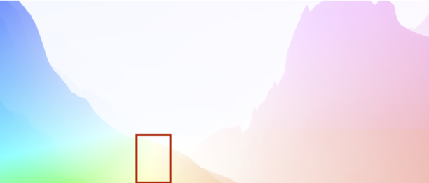
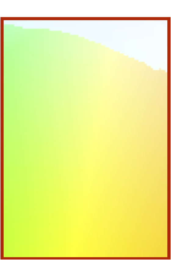
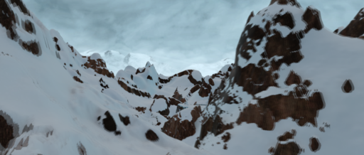
	Ground truth		Overlay of the input images
Our method
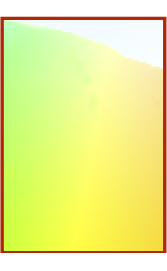
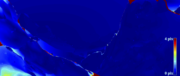
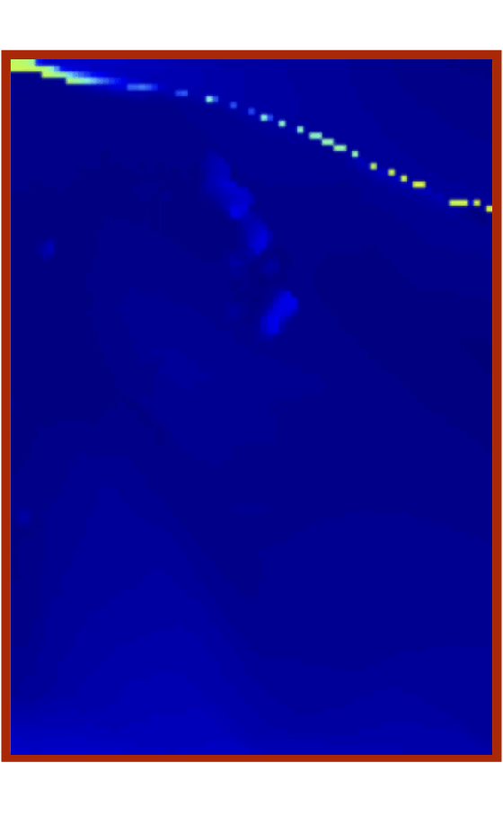
			$\text{AEP}=0.15$
Ours-TV
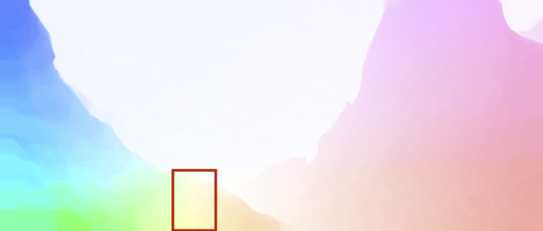
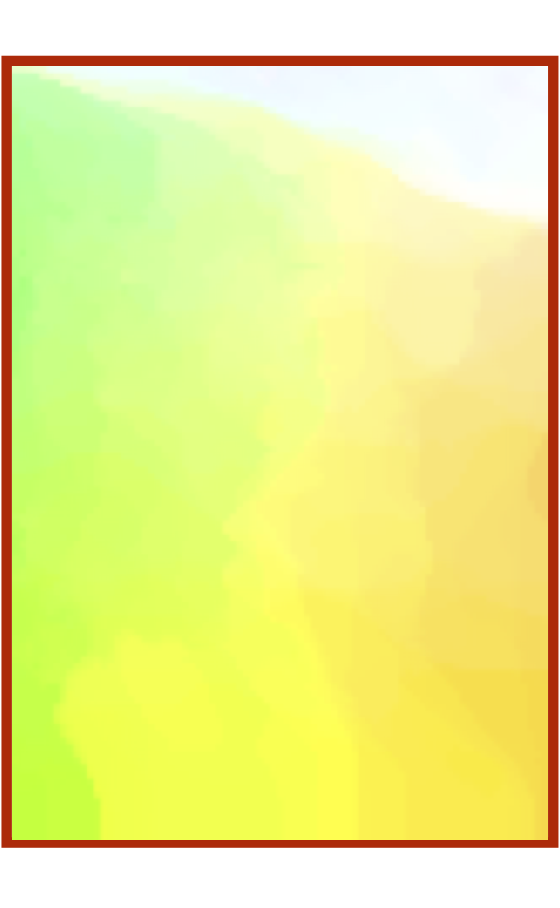
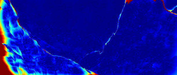
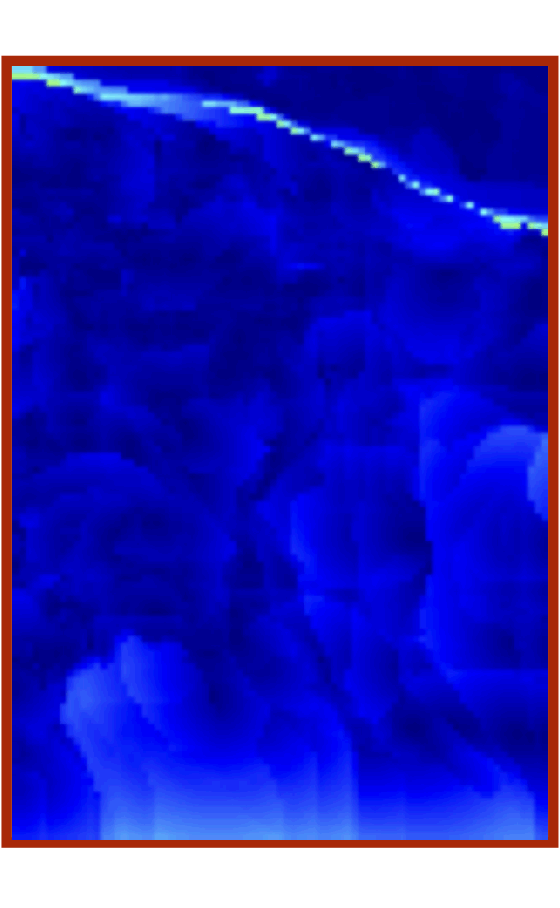
			$\text{AEP}=0.26$
Classic++
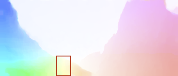
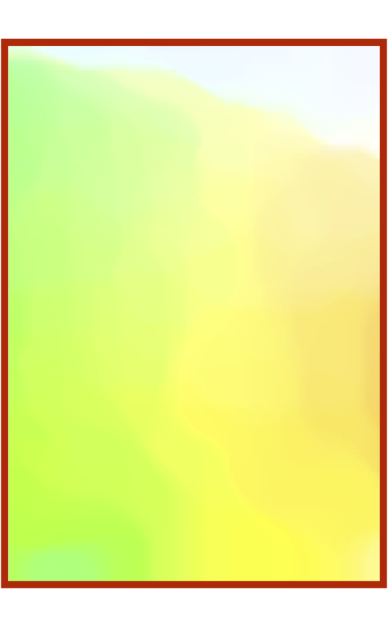
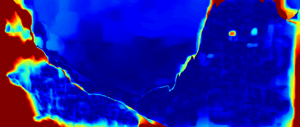
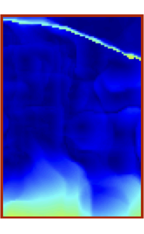
			$\text{AEP}=0.99$
Classic+NL
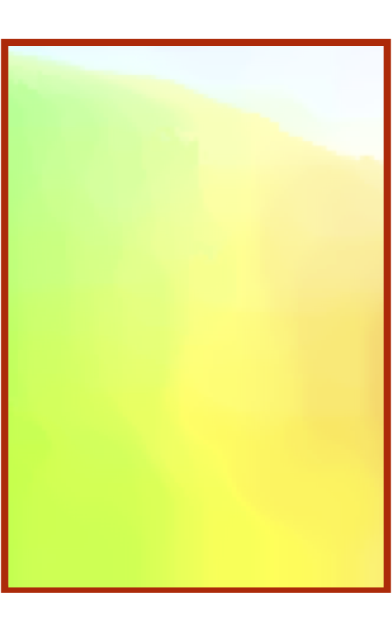
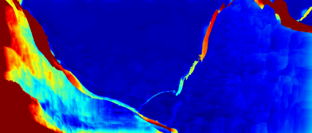
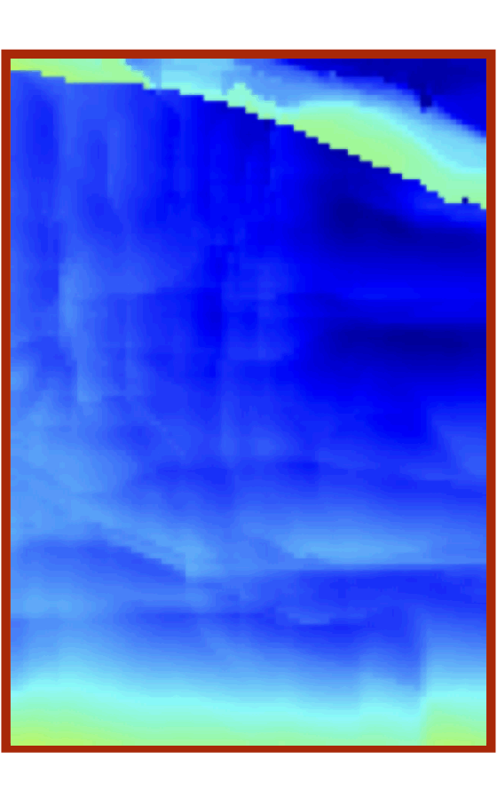
			$\text{AEP}=0.96$

Figure 1: Comparison of the TV motion fields (left column) and their associated error maps (right column). We provide a zoomed cutout of the motion field in each case.

TGV-Based Methods  The second-order TGV regularization generalizes the TV approach and imposes a piecewise-affine form by introducing penalization of second derivatives with an $\ell_{1}$ norm [4]. We consider the method $DataFlow$ described in [44]. It uses TGV regularization with several advanced data terms. In our experiments, we used the sum of absolute differences, which is a patch-based version of brightness constancy. We integrated $\phi$ from (22) in DataFlow, taking advantage of the public code provided by the authors.

We also performed comparisons with the nonlocal version of TGV proposed in [29], termed NL-TGV. However, the data term in NL-TGV is different from ours. It is based on the census transform, which provides invariance to illumination changes.

Piecewise-Parametric Methods  The method termed PH-Flow estimates a piecewise homography model and is based on the formulation (1) with inter-piece regularization and graph cut optimization [55].

We also perform comparisons with the method FC-2Layers-FF [40], which is based on a layered representation and is not purely piecewise-parametric but allows deviations from an affine model in each of the segmented region.

We used the publicly available codes for Classic++ and Classic+NL, $DeepFlow$, and $DataFlow$.

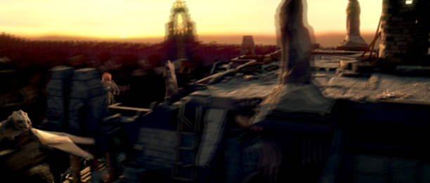
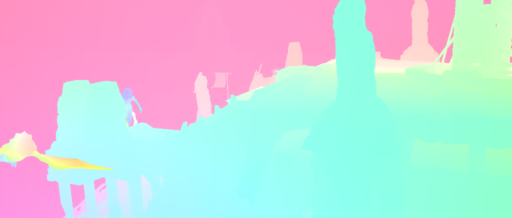
Overlay of the input images	Ground truth	Our method
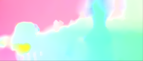
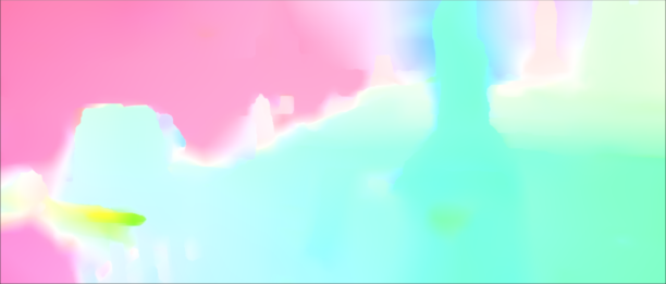
TGV-Census	NLTGV-Census	DataFlow
(extracted from [29])	(extracted from [29])

Figure 2: Comparison of the TGV motion fields. The visualizations of TGV-Census and NLTGV-Census are taken from [29]. The input images are from the $final$ version of the MPI Sintel dataset.

IV-D Evaluation Datasets

We validate our method on two reference benchmarks for motion estimation.

The MPI Sintel benchmark is composed of sequences extracted from a realistic animated movie. It contains $1\,064$ training sequences with available ground truth and 564 test sequences used for blind evaluation [7]. Each sequence has a final and a clean version. The final version introduces perturbations such as motion blur, defocus, or atmospheric fog, which are not present in the clean version. These effects are handled by the data term or by specific estimation strategies. To focus on the evaluation of the regularization, we used the clean dataset in our experiments.

The Kitti benchmark [16] is composed of 193 training sequences and 193 test sequences, acquired in real outdoor conditions on a platform installed on a moving car. A ground truth is provided only for half of the pixels. This benchmark is characterized by large illumination changes.

We compute the estimation accuracy with the endpoint error, defined at each pixel as the Euclidean distance between the estimated motion vector and the ground truth. We report the averaged endpoint error (AEP) on the whole image. To isolate the impact of the regularization, all the errors reported in this section have been computed in non-occluded regions. Occlusion handling is a separate problem that requires dedicated techniques not discussed in this paper [14, 22, 52, 53].

The results on the two benchmarks are presented in Table I, on the training and test sets. We consider methods with public codes for the training set, and the ones with published results for the test set. Therefore, some methods are not present in both categories. We did not report the result of DataFlow for the test set of MPI Sintel since the published results have been obtained without the large displacement extension of Section IV-A, which is decisive to obtain comparable results.

IV-E TV and TGV regularization

In Figure 1, we compare our result with methods based on TV regularization, namely, Ours-TV, Classic++, and its nonlocal variant Classic+NL, in the case of smooth variations of the motion field and small displacements. We display the estimated motion field and the endpoint error maps. The TV regularization produces typical staircasing artifacts due to the piecewise constancy of the solution. This effect is emphasized in the cutouts of Figure 1. Our piecewise-affine approach does not produce staircasing and is much closer to the ground truth, both visually and in terms of AEP. We also observe that the motion discontinuities are more accurately recovered with our approach.

In Figure 2, we compare our method with the methods TGV-Census, NLTGV-Census and DataFlow, which are based on TGV regularization. The absence of staircasing of TGV comes at the price of some blurring artifacts in the result. Even the nonlocal approach NLTGV-Census, which is specifically designed to reduce blurring, cannot solve completely the problem. In contrast, our method combines a good restitution of affine displacements with a satisfactory recovery of sharp motion discontinuities.

In Figure 3, we compare the results of our method, Ours-TV, $DeepFlow$ and $DataFlow$. We recall that the essential difference between these methods is only the regularization strategy. We observe that the sharpness of discontinuities is always better preserved in our results compared to $DeepFlow$ and $DataFlow$. Generally, the global shapes of moving objects are more accurately delineated by our method. We also observe staircasing artifacts in the results of Ours-TV. Altogether, the best AEP is achieved by our method. Note that large errors at image borders are due to occlusions and are not taken into account in the computation of the AEP.

These qualitative observations are confirmed by the better results of our approach in Table I compared to the methods with a similar framework but different regularization: Ours-TV, DeepFlow, DataFlow, Classic+NL, and NLTGV-Census.

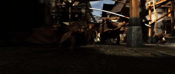
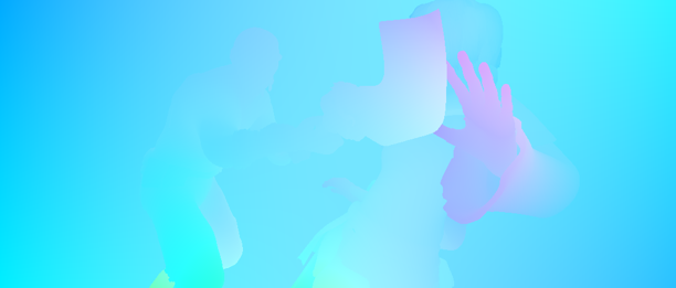
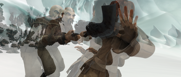
	Ground truth	Input images	Ground truth	Input Images
Our method
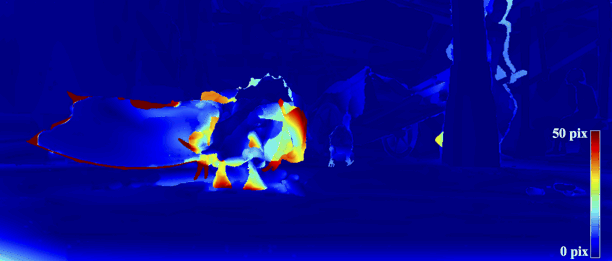
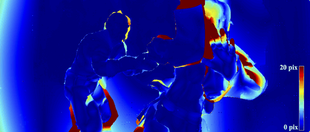
		$\text{AEP}=1.55$		$\text{AEP}=1.30$
Ours-TV
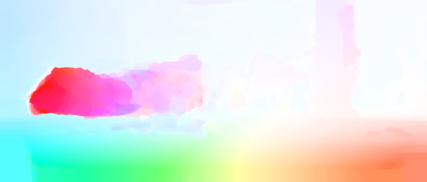
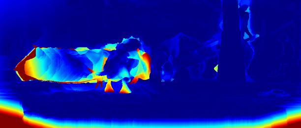
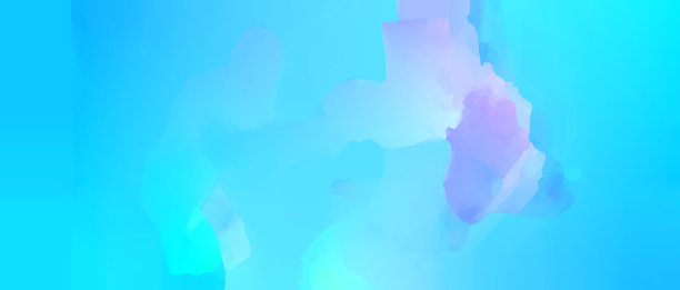
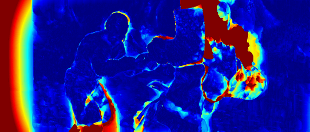
		$\text{AEP}=2.02$		$\text{AEP}=1.95$
DeepFlow
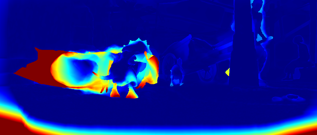
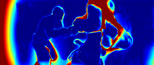
		$\text{AEP}=3.98$		$\text{AEP}=2.01$
DataFlow
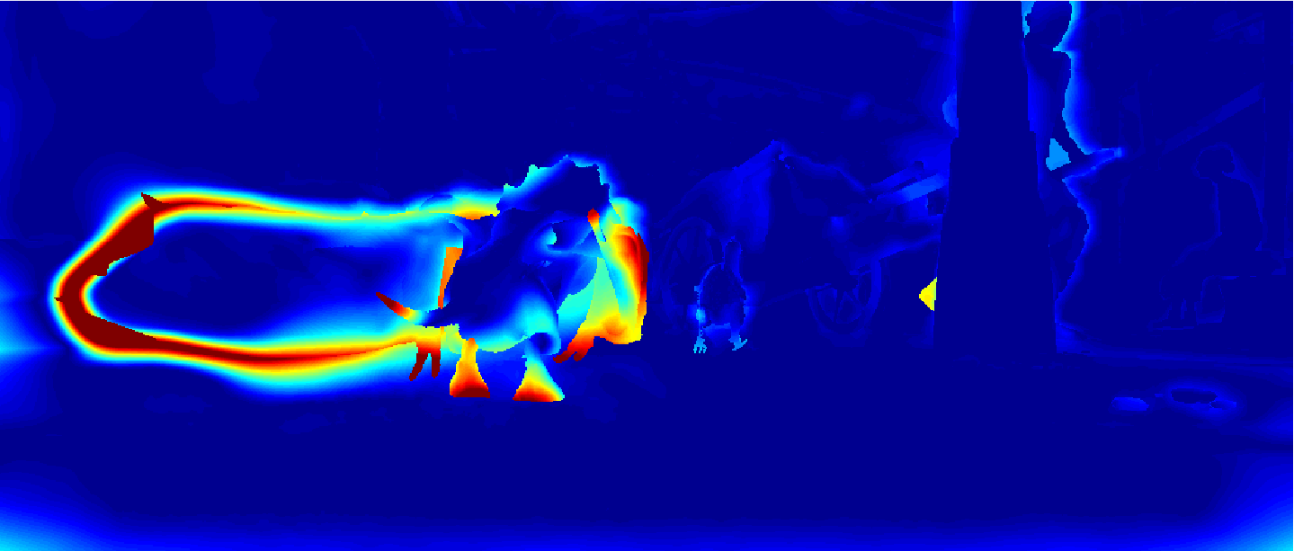
		$\text{AEP}=2.34$		$\text{AEP}=1.90$

Figure 3: Comparison of the motion fields (columns 1 and 3) and their associate error maps (columns 2 and 4) on the sequences market_4 (columns 1 and 2) and ambush_2 (columns 3 and 4) of the MPI Sintel benchmark.

IV-F Piecewise-Parametric Methods

In Figure 4, we show visual comparisons between our method, PH-Flow, and FC-2Layers-FF. On these examples, our method is able to retrieve more details and to delineate motion discontinuities more accurately. The numerical results of Table I show a clear advantage of our method on MPI Sintel. On the Kitti benchmark, our method is close to the best performing method PH-Flow.

Besides these numerical results, our method has four main practical advantages: (i) it is initialization-free, contrarily to other piecewise-parametric motion estimation methods; (ii) it is refinement-free, while the results of PH-Flow are obtained after refinement with the method Classic+NL dedicated to small displacements; (iii) it is fast, taking around 3 minutes on the non-downsampled images of the Kitti benchmark, while the reported computation time of PH-FLow is 15 minutes on the same benchmark, despite a downsampling by a factor of 2 in [55]; (iv) its running time is completely independent of the complexity of the flow field, while the running time of [55] is depends highly on the complexity of the motion field due to its need for an explicit motion segmentation.

Input images
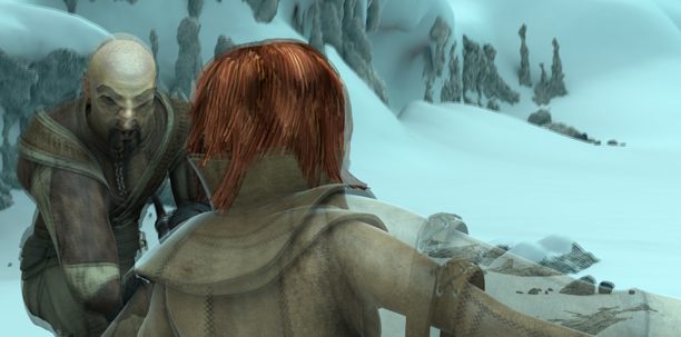
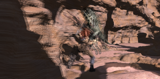
Ground truth
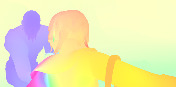
Our method
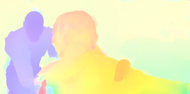
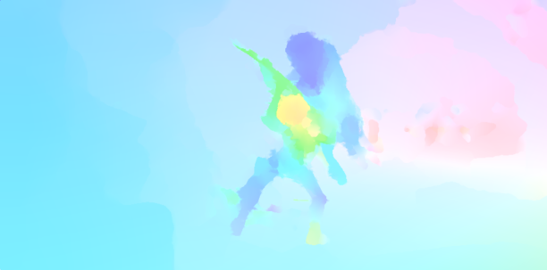
	$\text{AEP}=3.60$	$\text{AEP}=0.34$
PH-Flow
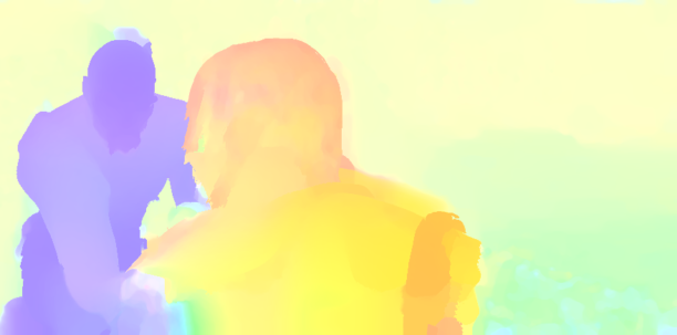
	$\text{AEP}=4.11$	$\text{AEP}=0.47$
FC-2Layers-FF
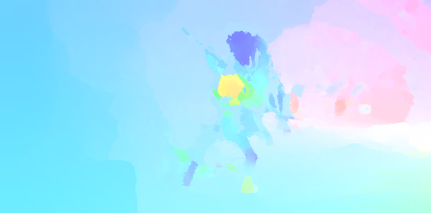
	$\text{AEP}=7.99$	$\text{AEP}=0.56$

Figure 4: Comparisons between the results of our method, PH-Flow [55], and FC-2Layers-FF [40] on images from the test sequence of the MPI Sintel benchmark.

IV-G Reconstitution of Piecewise-Affine Edges

To illustrate the piecewise-affine form of the estimated motion fields, we show in Figure 5 a reconstruction of motion edges obtained by thresholding the magnitude of spatial derivatives of the motion field. When the scene is composed of a few moving parts undergoing simple deformations, the image domain is divided in a few meaningful regions. When the motion is more complex, our method decomposes the motion field in smaller pieces. A crucial aspect of our method is that this increasing complexity has no effect on the computational cost.

Input images
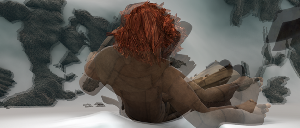
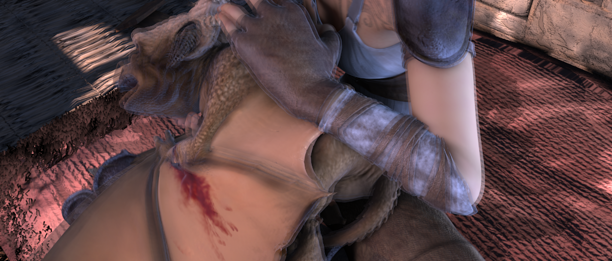
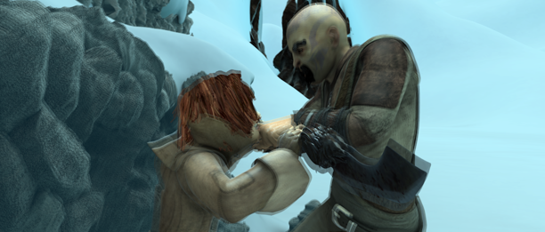
Ground truth
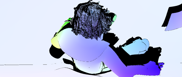
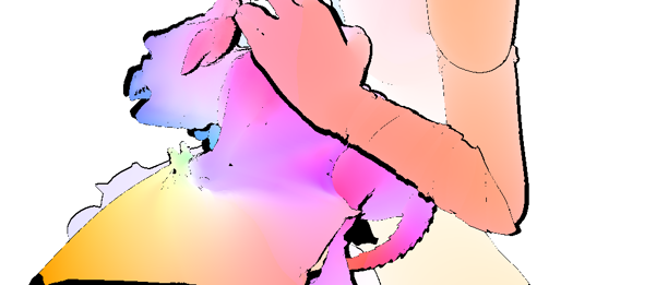
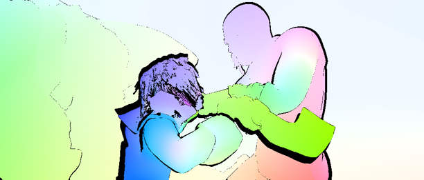
Motion field
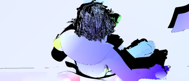
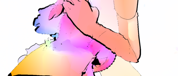
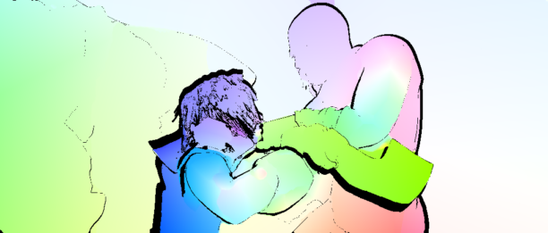
Motion edges

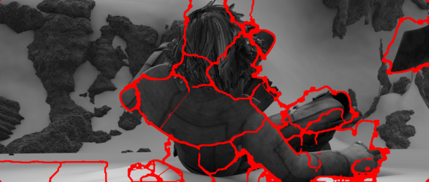
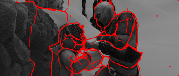
Figure 5: Reconstruction of motion edges (last row) from the motion field estimated with our method (third row) on examples of the MPI Sintel dataset. Black pixels in the motion fields represent occluded region.

V Conclusion

We have proposed a new method to estimate piecewise-affine motion fields. In contrast to related methods, our approach does not rely on explicit segmentation but directly estimates a piecewise-affine motion field. Key steps in the derivation are the specific formulation of the energy functional as a constrained optimization problem and the decomposition into tractable subproblems by an alternatig direction method of multipliers strategy. Then, these subproblems are cast to (non-convex) univariate piecewise-affine problems. A crucial ingredient of our method is that we are able to solve them exactly and efficiently. Our method overcomes the two main limitations of previous piecewise-parametric approaches, namely, sensitivity to initialization and computational cost. Yet, our experiments show that it is competitive in terms of quality. Further, they suggest that the piecewise affine model improves upon total variation and total generalized variation regularizations when using similar data terms. The versatility of our proximal splitting strategy lets extensions of the method to new data terms be easily implemented. Thus, the proposed approach can serve as a general regularization framework for motion estimation.

Appendix A Calculation of the Approximation Errors

We describe how to efficiently compute the approximation errors $\epsilon_{lrt}$ required in (20). Let $g\in\mathbb{R}^{n\times 2}.$ (This corresponds to $g_{pt}=v_{t}(x_{1},p).$ for all $p,t$ in (20).) Taking the derivative of the right-hand side of (21) with respect to $a,b$ yields the optimality conditions

$$\sum_{p=l}^{r}w_{p}(a_{lrt}p+b_{lrt}-g_{pt})p=0$$

$$\sum_{p=l}^{r}w_{p}(a_{lrt}p+b_{lrt}-g_{pt})=0.$$ (26)

This linear system can be rewritten as

$$a_{k}E_{lr}+b_{k}G_{lr}=I_{lrt},$$

$$a_{k}G_{lr}+b_{k}H_{lr}=J_{lrt},$$ (27)

with the auxiliary quantities

$$E_{lr}=\sum_{p=l}^{r}w_{p}p^{2},\quad G_{lr}=\sum_{p=l}^{r}w_{p}p,\quad H_{lr}=\sum_{p=l}^{r}w_{p},$$ (28)

$$I_{lrk}=\sum_{p=l}^{r}w_{p}g_{pt}p,\quad J_{lrk}=\sum_{p=l}^{r}w_{p}g_{pt}.$$ (29)

The solutions $a^{*}_{lrk}$ and $b^{*}_{lrk}$ are given by

$$a^{*}_{lrt}=\frac{I_{lr}H_{lr}-G_{lr}J_{lrk}}{E_{lr}H_{lr}-G_{lr}^{2}}$$ (30)

and

$$b^{*}_{lrt}=\frac{E_{lr}J_{lr}-I_{lrk}G_{lr}}{E_{lr}H_{lr}-G_{lr}^{2}}.$$ (31)

Plugging this into (21) gives us

$$\epsilon_{lrk}=\frac{J_{lr}^{2}E_{lr}-2G_{lr}J_{lrt}I_{lrt}+H_{lr}I_{lrt}^{2}+G_{lr}^{2}K_{lrt}-H_{lr}E_{lr}K_{lrt}}{G_{lr}^{2}-H_{lr}E_{lr}}$$ (32)

where $K_{lrt}=\sum_{p=l}^{r}w_{p}g_{pt}^{2}.$ Note that the involved sums can be computed efficiently by utilizing precomputations of moments. For example, $E_{lr}$ can be computed via $E_{lr}=E^{\prime}_{r}-E^{\prime}_{l-1}$ where $E^{\prime}_{t}=\sum_{p=1}^{t}w_{p}p^{2}.$ So $E_{lr}$ can be computed in $O(1)$ if the vector $E^{\prime}$ is precomputed. $E^{\prime}$ in turn can be computed in $O(n).$ For the other summations, analogous schemes are applied.

Appendix B Optimization for the Large Displacement Model

To solve the minimization problem (22) for the extended model, we follow the splitting scheme used for (III-B). We introduce an additional splitting variable associated to the term $\phi$. Accordingly, (22) rewrites

$$J=\min_{{\bf w},{\bf u},{\bf P}_{1},\ldots,{\bf P}_{K}}\left(\rho({\bf w})+\gamma\,\phi({\bf u},{\bf m})+\lambda\sum_{k=1}^{K}\alpha_{k}\|\mbox{\boldmath{$\nabla$}}_{d_{k}}{\bf P}_{k}\|_{0}\right)$$

$$\text{ s.t. }{\bf w}({\bf x})={\bf z}_{k}({\bf x}),$$

$$\phantom{\text{ s.t. }}{\bf u}({\bf x})={\bf w}({\bf x}),$$

$$\phantom{\text{ s.t. }}{\bf z}_{k}({\bf x})={\bf P}_{k}({\bf x})\bar{\bf x},\leavevmode\nobreak\ \forall{\bf x}\in\Omega,\leavevmode\nobreak\ \forall k=1,\ldots,K.$$

The augmented Lagrangian associated to (B) is then

$$\begin{split}\mathcal{A}_{\eta_{1},\eta_{2}}&({\bf w},{\bf u},\{{\bf P}_{k}\}_{k},\{{\bf z}_{k}\}_{k},\{\mbox{\boldmath{$\upmu$}}_{k}\}_{k},\mbox{\boldmath{$\upxi$}})=\\ &\rho({\bf w})+\gamma\,\phi({\bf u},{\bf m})+\lambda\sum_{k=1}^{K}\alpha_{k}\|\mbox{\boldmath{$\nabla$}}_{{\bf d}_{k}}{\bf P}_{k}\|_{0}\\ &+\frac{\eta_{1}}{2}\sum_{k=1}^{K}\sum_{{\bf x}\in\Omega}\left\|{\bf w}({\bf x})-{\bf z}_{k}({\bf x})+\frac{\mbox{\boldmath{$\upmu$}}_{k}({\bf x})}{\eta_{1}}\right\|_{2}^{2}-\frac{1}{2\eta_{1}}\left\|\mbox{\boldmath{$\upmu$}}_{k}({\bf x})\right\|_{2}^{2}\\ &+\frac{\eta_{2}}{2}\sum_{{\bf x}\in\Omega}\left\|{\bf u}({\bf x})-{\bf w}({\bf x})+\frac{\mbox{\boldmath{$\upxi$}}({\bf x})}{\eta_{2}}\right\|_{2}^{2}-\frac{1}{2\eta_{2}}\left\|\mbox{\boldmath{$\upxi$}}({\bf x})\right\|_{2}^{2}\\[4.30554pt] \text{ s.t. }&{\bf z}_{k}({\bf x})={\bf P}_{k}({\bf x})\bar{\bf x},\leavevmode\nobreak\ \forall{\bf x}\in\Omega,\leavevmode\nobreak\ \forall k\in\{1,\ldots,K\}.\end{split}$$ (34)

Similarly to the update scheme (III-B), the ADMM steps involve minimizing $\mathcal{A}_{\eta_{1},\eta_{2}}({\bf w},{\bf u},\{{\bf P}_{k}\}_{k},\{{\bf z}_{k}\}_{k},\{\mbox{\boldmath{$\upmu$}}_{k}\}_{k},\mbox{\boldmath{$\upxi$}})$ with respect to ${\bf w}$, ${\bf z}_{k}$, and ${\bf u}$. The minimization problem with respect to ${\bf z}_{k}$ is the same as in Section III-D. We detail now the updates of ${\bf w}$ and ${\bf u}$, which are very similar to the description of Section III-C.

Update of ${\bf w}$

The minimization w.r.t $u$ in can be rewritten

$$\min_{\bf w}\rho({\bf w})\leavevmode\nobreak\ +\leavevmode\nobreak\ \frac{\eta_{1}K+\eta_{2}}{2}\sum_{{\bf x}\in\Omega}\left({\bf w}({\bf x})-{\bf t}({\bf x})\right)^{2},$$ (35)

where

$${\bf t}({\bf x})=\frac{1}{\eta_{1}K+\eta_{2}}\left(\eta_{1}K\ {\bf r}({\bf x})+\eta_{2}\left({\bf u}({\bf x})+\frac{\mbox{\boldmath{$\upxi$}}({\bf x})}{\eta_{2}}\right)\right).$$ (36)

The problem is pointwise and admits a closed-form solution with the thresholding scheme

$${\bf w}({\bf x})={\bf t}({\bf x})+\begin{cases}\frac{\mbox{\boldmath{$\nabla$}}I}{\eta_{1}K},&\rho_{0}({\bf t}({\bf x}))<-\frac{\|\mbox{\boldmath{$\nabla$}}I\|_{2}^{2}}{\eta_{1}K}\\ -\frac{\mbox{\boldmath{$\nabla$}}I}{\eta_{1}K},&\rho_{0}({\bf t}({\bf x}))>\frac{\|\mbox{\boldmath{$\nabla$}}I\|_{2}^{2}}{\eta_{1}K}\\ -\rho_{0}({\bf t}({\bf x}))\frac{\mbox{\boldmath{$\nabla$}}I}{\|\mbox{\boldmath{$\nabla$}}I\|_{2}^{2}},&|\rho_{0}({\bf t}({\bf x}))|\leq\frac{\|\mbox{\boldmath{$\nabla$}}I\|_{2}^{2}}{\eta_{1}K}.\end{cases}$$ (37)

Update of ${\bf u}$

The minimization w.r.t $u$ in writes

$$J=\min_{\bf u}\left(\gamma\phi({\bf u},{\bf m})+\frac{\eta_{2}}{2}\sum_{{\bf x}\in\Omega}\left\|{\bf u}({\bf x})-{\bf v}({\bf x})\right\|^{2}\right).$$ (38)

where ${\bf v}({\bf x})={\bf w}({\bf x})-\frac{\mbox{\boldmath{$\upxi$}}({\bf x})}{\eta_{2}}$.

The problem is pointwise and admits a closed-form solution with the thresholding scheme

$$u_{k}({\bf x})=\begin{cases}v_{k}({\bf x}),&c({\bf x})=0,\\ v_{k}({\bf x})+\frac{\gamma}{\eta_{2}},&v_{k}({\bf x})-m_{k}({\bf x})<-\frac{\gamma}{\eta_{2}}\text{ and }c({\bf x})\neq 0\\ v_{k}({\bf x})-\frac{\gamma}{\eta_{2}},&v_{k}({\bf x})-m_{k}({\bf x})>\frac{\gamma}{\eta_{2}}\text{ and }c({\bf x})\neq 0\\ m_{k}({\bf x}),&|v_{k}({\bf x})-m_{k}({\bf x})|\leq\frac{\gamma}{\eta_{2}}\text{ and }c({\bf x})\neq 0.\end{cases}$$ (39)

where $k=\{1,2\}$ and we use the notations ${\bf u}({\bf x})=(u_{1}({\bf x}),u_{2}({\bf x}))$, ${\bf v}({\bf x})=(v_{1}({\bf x}),v_{2}({\bf x}))$, and ${\bf m}({\bf x})=(m_{1}({\bf x}),m_{2}({\bf x}))$.

References

- [1] A. Blake and A. Zisserman. Visual reconstruction. MIT Press Cambridge, 1987.
- [2] M. Bleyer, C. Rhemann, and M. Gelautz. Segmentation-based motion with occlusions using graph-cut optimization. In DAGM Symposium on Pattern Recognotion, pages 465–474, Berlin, Germany, September 2006.
- [3] Patrick Bouthemy and Edouard François. Motion segmentation and qualitative dynamic scene analysis from an image sequence. Int. J. of Computer Vision, 10(2):157–182, 1993.
- [4] Kristian Bredies, Karl Kunisch, and Thomas Pock. Total generalized variation. SIAM Journal on Imaging Sciences, 3(3):492–526, 2010.
- [5] T. Brox, A. Bruhn, N. Papenberg, and J. Weickert. High accuracy optical flow estimation based on a theory for warping. In European Conference on Computer Vision (ECCV), pages 25–36, Prague, Czech Republic, 2004.
- [6] T. Brox and J. Malik. Large displacement optical flow: descriptor matching in variational motion estimation. IEEE Trans. Pattern Analysis and Machine Intelligence, 33(3):500–513, 2011.
- [7] D. Butler, J. Wulff, G. Stanley, and M. Black. A naturalistic open source movie for optical flow evaluation. In European Conference on Computer Vision (ECCV), pages 611–625. Springer-Verlag, 2012.
- [8] Xiaohao Cai, Jan Henrik Fitschen, Mila Nikolova, Gabriele Steidl, and Martin Storath. Disparity and optical flow partitioning using extended potts priors. Information and Inference, 4(1):43–62, 2015.
- [9] A. Chambolle. Finite-differences discretizations of the Mumford-Shah functional. ESAIM: Mathematical Modelling and Numerical Analysis, 33(02):261–288, 1999.
- [10] A. Chambolle and T. Pock. A first-order primal-dual algorithm for convex problems with applications to imaging. Journal of Mathematical Imaging and Vision, 40(1):120–145, 2011.
- [11] Rick Chartrand and Brendt Wohlberg. A nonconvex ADMM algorithm for group sparsity with sparse groups. In International Conference on Acoustics, Speech and Signal Processing (ICASSP), pages 6009–6013, 2013.
- [12] L. Condat. A direct algorithm for 1-D total variation denoising. IEEE Signal Processing Letters, 20(11):1054–1057, 2013.
- [13] D. Cremers and S. Soatto. Motion competition: A variational approach to piecewise parametric motion segmentation. Int. J. of Computer Vision, 62(3):249–265, 2005.
- [14] Denis Fortun, Patrick Bouthemy, and Charles Kervrann. Aggregation of local parametric candidates with exemplar-based occlusion handling for optical flow. Computer Vision and Image Understanding, 145:81–94, 2016.
- [15] F. Friedrich, A. Kempe, V. Liebscher, and G. Winkler. Complexity penalized M-estimation. Journal of Computational and Graphical Statistics, 17(1):201–224, 2008.
- [16] Andreas Geiger, Philip Lenz, and Raquel Urtasun. Are we ready for autonomous driving? the KITTI vision benchmark suite. In Computer Vision and Pattern Recognition (CVPR), pages 3354–3361, 2012.
- [17] Raja Giryes, Michael Elad, and Alfred M Bruckstein. Sparsity based methods for overparameterized variational problems. SIAM Journal on Imaging Sciences, 8(3):2133–2159, 2015.
- [18] K. Hohm, M. Storath, and A. Weinmann. An algorithmic framework for Mumford-Shah regularization of inverse problems in imaging. Inverse Problems, 31(11):115011, 2015.
- [19] B.K.P. Horn and B.G. Schunck. Determining optical flow. Artificial Intelligence, 17(1-3):185–203, 1981.
- [20] Michael Hornacek, Frederic Besse, Jan Kautz, Andrew W. Fitzgibbon, and Carsten Rother. Highly overparameterized optical flow using patchmatch belief propagation. In European Conference on Computer Vision, Zurich,, pages 220–234, 2014.
- [21] Junhwa Hur and Stefan Roth. Joint optical flow and temporally consistent semantic segmentation. ECCV, 2016.
- [22] Serdar Ince and Janusz Konrad. Occlusion-aware optical flow estimation. IEEE Trans. Image Processing, 17(8):1443–1451, 2008.
- [23] Jon Kleinberg and Eva Tardos. Algorithm design. Pearson Education India, 2006.
- [24] E. Memin and P. Perez. Hierarchical estimation and segmentation of dense motion fields. Int. J. of Computer Vision, 46(2):129–155, 2002.
- [25] D. Mumford and J. Shah. Optimal approximations by piecewise smooth functions and associated variational problems. Communications on Pure and Applied Mathematics, 42(5):577–685, 1989.
- [26] Tal Nir, Alfred M Bruckstein, and Ron Kimmel. Over-parameterized variational optical flow. Int. J. of Computer Vision, 76(2):205–216, 2008.
- [27] J.M. Odobez and P. Bouthemy. Direct incremental model-based image motion segmentation for video analysis. Signal Processing, 66(2):143–155, 1998.
- [28] Nikos Paragios and Rachid Deriche. Geodesic active regions and level set methods for motion estimation and tracking. Computer Vision and Image Understanding, 97(3):259–282, 2005.
- [29] R Ranftl, K. Bredies, and T. Pock. Non-local total generalized variation of optical flow estimation. In European Conference on Computer Vision, pages 439–454, Zurich, 2015.
- [30] J. Revaud, P. Weinzaepfel, and C Harchoui, Z. Schmid. Epicflow: Edge-preserving interpolation of correspondences for optical flow. In IEEE Conf. Computer Vision and Pattern Recognition (CVPR’15), Boston, MA, 2015.
- [31] Thomas Schoenemann and Daniel Cremers. Near real-time motion segmentation using graph cuts. In DAGM Symposium on Pattern Recognition, pages 455–464, 2006.
- [32] Laura Sevilla-Lara, Deqing Sun, Varun Jampani, and Michael J Black. Optical flow with semantic segmentation and localized layers. CVPR, 2016.
- [33] M. Storath and A. Weinmann. Fast partitioning of vector-valued images. SIAM Journal on Imaging Sciences, 7(3):1826–1852, 2014.
- [34] M. Storath, A. Weinmann, and L. Demaret. Jump-sparse and sparse recovery using Potts functionals. IEEE Transactions on Signal Processing, 62(14):3654–3666, 2014.
- [35] M. Storath, A. Weinmann, J. Frikel, and M. Unser. Joint image reconstruction and segmentation using the Potts model. Inverse Problems, 31(2):025003, 2015.
- [36] D. Sun, S. Roth, and M.J. Black. Secrets of optical flow estimation and their principles. In Computer Vision and Pattern Recognition (CVPR), pages 2432–2439, San Fransisco, June 2010.
- [37] D. Sun, E. Sudderth, and M. Black. Layered image motion with explicit occlusions, temporal consistency, and depth ordering. In Advances in Neural Information Processing Systems (NIPS), pages 2226–2234, Vancouver, Canada, 2010.
- [38] Deqing Sun, Stefan Roth, and Michael Black. A quantitative analysis of current practices in optical flow estimation and the principles behind them. Int. J. of Computer Vision, 106(2):115–137, 2014.
- [39] Deqing Sun, Erik Sudderth, and Michael Black. Layered segmentation and optical flow estimation over time. In Computer Vision and Pattern Recognition (CVPR), pages 1768–1775, 2012.
- [40] Deqing Sun, Jonas Wulff, Erik Sudderth, Hanspeter Pfister, and Michael Black. A fully-connected layered model of foreground and background flow. In IEEE Conf. Computer Vision and Pattern Recognition (CVPR), pages 2451–2458, 2013.
- [41] W. Trobin, T. Pock, D. Cremers, and H. Bischof. An unbiased second-order prior for high-accuracy motion estimation. DAGM Symposium on Pattern Recognition, pages 396–405, 2008.
- [42] Markus Unger, Manuel Werlberger, Thomas Pock, and Horst Bischof. Joint motion estimation and segmentation of complex scenes with label costs and occlusion modeling. In Computer Vision and Pattern Recognition (CVPR), pages 1878–1885, 2012.
- [43] Carlos Vazquez, Amar Mitiche, and Robert Laganiere. Joint multiregion segmentation and parametric estimation of image motion by basis function representation and level set evolution. IEEE Transactions on Pattern Analysis and Machine Intelligence, 28(5):782–793, 2006.
- [44] Christoph Vogel, Stefan Roth, and Konrad Schindler. An evaluation of data costs for optical flow. In DAGM Symposium on Pattern Recognition, pages 343–353, 2013.
- [45] Christoph Vogel, Konrad Schindler, and Stefan Roth. 3d scene flow estimation with a piecewise rigid scene model. International Journal of Computer Vision, 115(1):1–28, 2015.
- [46] John Wang and Edward Adelson. Representing moving images with layers. IEEE Trans. Image Processing, 3(5):625–638, 1994.
- [47] Yu Wang, Wotao Yin, and Jinshan Zeng. Global convergence of ADMM in nonconvex nonsmooth optimization. Preprint arXiv:1511.06324, 2015.
- [48] A. Weinmann and M. Storath. Iterative Potts and Blake-Zisserman minimization for the recovery of functions with discontinuities from indirect measurements. Proceedings of the Royal Society of London A: Mathematical, Physical and Engineering Sciences, 471(2176):20140638, 2015.
- [49] P. Weinzaepfel, J. Revaud, Z. Harchaoui, C. Schmid, et al. Deepflow: Large displacement optical flow with deep matching. In Int. Conf. on Computer Vision (ICCV), pages 1385–1392, Sydney, 2013.
- [50] M. Werlberger, W. Trobin, T. Pock, A. Wedel, D. Cremers, and H. Bischof. Anisotropic Huber-L1 optical flow. In British Machine Vision Conference (BMVC), 2009.
- [51] G. Winkler and V. Liebscher. Smoothers for discontinuous signals. Journal of Nonparametric Statistics, 14(1-2):203–222, 2002.
- [52] Jiangjian Xiao, Hui Cheng, Harpreet Sawhney, Cen Rao, and Michael Isnardi. Bilateral filtering-based optical flow estimation with occlusion detection. In European Conference on Computer Vision (ECCV), pages 211–224, 2006.
- [53] Li Xu, Jiaya Jia, and Yasuyuki Matsushita. Motion detail preserving optical flow estimation. IEEE Trans. Pattern Analysis and Machine Intelligence, 34(9):1744–1757, 2012.
- [54] Zheng Xu, Soham De, Mario Figueiredo, Christoph Studer, and Tom Goldstein. An empirical study of ADMM for nonconvex problems. Preprint arXiv:1612.03349, 2016.
- [55] J. Yang and H. Li. Dense, accurate optical flow estimation with piecewise parametric model. In IEEE Conf. Computer Vision and Pattern Recognition (CVPR), Boston, MA, 2015.
- [56] C. Zach, T. Pock, and H. Bischof. A duality based approach for realtime TV-L1 optical flow. In DAGM Symposium on Pattern Recognition, pages 214–223, 2007.