Conformal Parametrisation of Loxodromes
by Triples of Circles

Abstract.

We provide a parametrisation of a loxodrome by three specially arranged cycles. The parametrisation is covariant under fractional linear transformations of the complex plane and naturally encodes conformal properties of loxodromes. Selected geometrical examples illustrate the usage of parametrisation. Our work extends the set of objects in Lie sphere geometry—circle, lines and points—to the natural maximal conformally-invariant family, which also includes loxodromes.

1. Introduction

It is easy to come across shapes of logarithmic spirals, as on Fig. 1(a), looking either on a sunflower, a snail shell or a remote galaxy. It is not surprising since the fundamental differential equation $\dot{y}=\lambda y$, $\lambda\in\mathbb{C}{}$ serves as a first approximation to many natural processes.

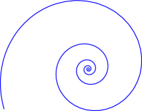
(a) (b)

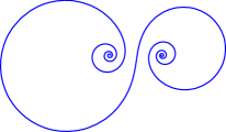
Figure 1. A logarithnic spiral (a) and its image under a fractional linear transformation—loxodrome (b).

The main symmetries of complex analysis are build on the fractional linear transformation (FLT):

(1) $$\begin{pmatrix}\alpha&\beta\\ \gamma&\delta\end{pmatrix}:\ z\mapsto\frac{\alpha z+\beta}{\gamma z+\delta},\quad\text{ where }\alpha,\beta,\gamma,\delta\in\mathbb{C}{}\text{ and }\det\begin{pmatrix}\alpha&\beta\\ \gamma&\delta\end{pmatrix}\neq 0.$$

Thus, images of logarithmic spirals under FLT, called loxodromes, as on Fig. 1(b) shall not be rare. Indeed, they appear in many occasions from the stereographic projection of a rhumb line in navigation to a preferred model of a Carleson arc in the theory singular integral operators [BoettcherKarlovich01a, BishopBoettcherKarlovichSpitkovsky99a]. Furthermore, loxodromes are orbits of one-parameter continuous groups of FLT of loxodromic type [Beardon95]*§ 4.3 [Simon11a]*§ 9.2 [Vasilevski08a]*§ 9.2.

This setup motivates a search for effective tools to deal with FLT-invariant properties of loxodromes. They were studied from a differential geometry point of view in several recent paper [Bolt07a, Porter93a, Porter98a, Porter98b, Porter07a]. In this work we develop a “global” description which matches the Lie sphere geometry framework, see Rem. 3.

The outline of the paper is as follows. After preliminaries on FLT and invariant geometry of cycles (Section 2) we review the basics of logarithmic spirals and loxodromes (Section 3). A new parametrisation of loxodromes is introduced in Section 4 and several examples illustrate its usage in Section 5. Section 6 frames our work within a wider approach [Kisil15a, Kisil14b], which extends Lie sphere geometry. A brief list of open questions concludes the paper.

2. Preliminaries: Fractional Linear Transformations and Cycles

In this section we provide some necessary background in Lie geometry of circles, fractional-linear transformations and Fillmore–Springer–Cnops construction (FSCc). Regretfully, the latter remains largely unknown in the context of complex numbers despite of its numerous advantages. We will have some further discussion of this in Rem. 3 below.

The right way [Simon11a]*§ 9.2 to think about FLT (1) is through the projective complex line $P\mathbb{C}{}$. It is the family of cosets in $\mathbb{C}^{2}{}$ with respect to the equivalence relation $\begin{pmatrix}w_{1}\\ w_{2}\end{pmatrix}\sim\begin{pmatrix}\alpha w_{1}\\ \alpha w_{2}\end{pmatrix}$ for all nonzero $\alpha\in\mathbb{C}{}$. Conveniently $\mathbb{C}{}$ is identified with a part of $P\mathbb{C}{}$ by assigning the coset of $\begin{pmatrix}z\\ 1\end{pmatrix}$ to $z\in\mathbb{C}{}$. Loosely speaking $P\mathbb{C}{}=\mathbb{C}{}\cup\{\infty\}$, where $\infty$ is the coset of $\begin{pmatrix}1\\ 0\end{pmatrix}$. The pair $[w_{1}:w_{2}]$ with $w_{2}\neq 0$ gives homogeneous coordinates for $z=w_{1}/w_{2}\in\mathbb{C}{}$. Then, the linear map $\mathbb{C}^{2}{}\rightarrow\mathbb{C}^{2}{}$

(2) $$M:\ \begin{pmatrix}w_{1}\\ w_{2}\end{pmatrix}\mapsto\begin{pmatrix}w_{1}^{\prime}\\ w_{2}^{\prime}\end{pmatrix}=\begin{pmatrix}\alpha w_{1}+\beta w_{2}\\ \gamma w_{1}+\delta w_{2}\end{pmatrix},\text{ where }M=\begin{pmatrix}\alpha&\beta\\ \gamma&\delta\end{pmatrix}\in\mathrm{GL}_{2}(\mathbb{C}{})$$

factors from $\mathbb{C}^{2}{}$ to $P\mathbb{C}{}$ and coincides with (1) on $\mathbb{C}{}\subset P\mathbb{C}{}$.

Generic equations of cycle in real and complex coordinates $z=x+\mathrm{i}y$ are:

(3) $$k(x^{2}+y^{2})-2lx-2ny+m=0\qquad\text{or}\qquad kz\bar{z}-\bar{L}z-{L}\bar{z}+m=0\,,$$

where $(k,l,n,m)\in\mathbb{R}^{4}{}$ and $L=l+\mathrm{i}n$. This includes lines (if $k=0$), points as zero-radius circles (if $l^{2}+n^{2}-mk=0$) and proper circles otherwise. Homogeneity of (3) suggests that $(k,l,m,n)$ shall be considered as homogeneous coordinates $[k:l:m:n]$ of a point in three-dimensional projective space $P\mathbb{R}^{3}{}$.

The homogeneous form of cycle’s equation (3) for $z=[w_{1}:w_{2}]$ can be written using matrices as follows:

(4) $$kw_{1}\bar{w}_{1}-\bar{L}w_{1}\bar{w}_{2}-{L}\bar{w}_{1}w_{2}+mw_{2}\bar{w}_{2}=\begin{pmatrix}-\bar{w}_{2}&\bar{w}_{1}\end{pmatrix}\begin{pmatrix}\bar{L}&-m\\ k&-{L}\end{pmatrix}\begin{pmatrix}{w}_{1}\\ w_{2}\end{pmatrix}=0.$$

From now on we identify a cycle $C$ given by (3) with its $2\times 2$ matrix $\begin{pmatrix}\bar{L}&-m\\ k&-{L}\end{pmatrix}$, this is called the Fillmore–Springer–Cnops construction (FSCc) . Again, $C$ shall be treated up to the equivalence relation $C\sim tC$ for all real $t\neq 0$. Then, the linear action (2) corresponds to some action on $2\times 2$ cycle matrices by the intertwining identity:

(5) $$\begin{pmatrix}-\bar{w}^{\prime}_{2}&\bar{w}^{\prime}_{1}\end{pmatrix}\begin{pmatrix}\bar{L}^{\prime}&-m^{\prime}\\ k^{\prime}&-{L}^{\prime}\end{pmatrix}\begin{pmatrix}{w}^{\prime}_{1}\\ w^{\prime}_{2}\end{pmatrix}=\begin{pmatrix}-\bar{w}_{2}&\bar{w}_{1}\end{pmatrix}\begin{pmatrix}\bar{L}&-m\\ k&-{L}\end{pmatrix}\begin{pmatrix}{w}_{1}\\ w_{2}\end{pmatrix}.$$

Explicitly, for $M\in\mathrm{GL}_{2}(\mathbb{C}{})$ those actions are:

(6) $$\begin{pmatrix}{w}^{\prime}_{1}\\ w^{\prime}_{2}\end{pmatrix}=M\begin{pmatrix}{w}_{1}\\ w_{2}\end{pmatrix},\quad\text{and}\quad\begin{pmatrix}\bar{L}^{\prime}&-m^{\prime}\\ k^{\prime}&-{L}^{\prime}\end{pmatrix}=\bar{M}\begin{pmatrix}\bar{L}&-m\\ k&-{L}\end{pmatrix}M^{-1}\,,$$

where $\bar{M}$ is the component-wise complex conjugation of $M$. Note, that FLT $M$ (1) corresponds to a linear transformation $C\mapsto M(C):=\bar{M}CM^{-1}$ of cycle matrices in (6). A quick calculation shows that $M(C)$ indeed has real off-diagonal elements as required for a FSCc matrix.

This paper essentially depends on the following

Proposition 1.

Define a cycle product of two cycles $C$ and $C^{\prime}$ by:

(7) $$\left\langle C,C^{\prime}\right\rangle:=\mathop{\mathrm{tr}}(C\bar{C}^{\prime})=L\bar{L}^{\prime}+\bar{L}L^{\prime}-mk^{\prime}-km^{\prime}.$$

Then, the cycle product is FLT-invariant:

(8) $$\left\langle M(C),M(C^{\prime})\right\rangle=\left\langle C,C^{\prime}\right\rangle\qquad\text{for any }M\in\mathrm{SL}_{2}(\mathbb{C}{})\,.$$

Proof.

Indeed:

$$\left\langle M(C),M(C^{\prime})\right\rangle =\mathop{\mathrm{tr}}(M(C)\overline{M(C^{\prime})})$$

$$=\mathop{\mathrm{tr}}(\bar{M}CM^{-1}M\bar{C}^{\prime}\bar{M}^{-1})$$

$$=\mathop{\mathrm{tr}}(\bar{M}C\bar{C}^{\prime}\bar{M}^{-1})$$

$$=\mathop{\mathrm{tr}}(C\bar{C}^{\prime})$$

$$=\left\langle C,C^{\prime}\right\rangle,$$

using the invariance of trace. ∎

Note that the cycle product (7) is not positive definite, it produces a Lorentz-type metric in $\mathbb{R}^{4}{}$. Here are some relevant examples of geometric properties expressed through the cycle product:

Example 2.

1. If $k=1$ (and $C$ is a proper circle), then $\left\langle C,C\right\rangle\!/2$ is equal to the square of radius of $C$. In particular $\left\langle C,C\right\rangle=0$ indicates a zero-radius circle representing a point.

2. If $\left\langle C_{1},C_{2}\right\rangle=0$ for non-zero radius cycles $C_{1}$ and $C_{2}$, then they intersects at the right angle.

3. If $\left\langle C_{1},C_{2}\right\rangle=0$ and $C_{2}$ is zero-radius circle, then $C_{1}$ passes the point represented by $C_{2}$.

In general, a combination of (6) and (8) yields that a consideration of FLT in $\mathbb{C}{}$ can be replaced by linear algebra in the space of cycles $\mathbb{R}^{4}{}$ (or rather $P\mathbb{R}^{3}{}$) with an indefinite metric, see [GohbergLancasterRodman05a] for the latter.

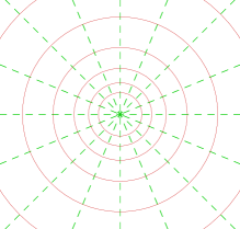
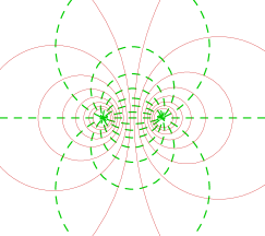
Figure 2. Orthogonal elliptic (green-dashed) and hyperbolic (red-solid) pencils of cycles. Left drawing shows the standard case and the right—generic, which is the image of the standard pencils under FLT.

A spectacular (and needed later) illustration of this approach is orthogonal pencils of cycles. Consider a collection of all cycles passing two different points in $\mathbb{C}{}$, it is called an elliptic pencil. A beautiful and non-elementary fact of the Euclidean geometry is that cycles orthogonal to every cycle in the elliptic pencil fill the entire plane and are disjoint, the family is called a hyperbolic pencil. The statement is obvious in the standard arrangement when the elliptic pencil is formed by straight lines—cycles passing the origin and infinity. Then, the hyperbolic pencil consists of the concentric circles, see Fig. 2. For the sake of completeness, a parabolic pencil (not used in this paper) formed by all circles touching a given line at a given point, [Kisil12a]*Ex. 6.10 contains further extensions and illustrations. See [Vasilevski08a]*§ 11.8 for an example of cycle pencils’ appearance in operator theory.

This picture trivialises a bit in the language of cycles. A pencil of cycles (of any type!) is a linear span $tC_{1}+(1-t)C_{2}$ of two arbitrary different cycles $C_{1}$ and $C_{2}$ from the pencil. Again, this is easier to check for the standard pencils. A pencil is elliptic, parabolic or hyperbolic depending on which inequality holds [Kisil12a]*Ex. 5.28.ii:

(9) $$\left\langle C_{1},C_{2}\right\rangle^{2}\lesseqqgtr\left\langle C_{1},C_{1}\right\rangle\left\langle C_{2},C_{2}\right\rangle.$$

Then, the orthogonality of cycles on the plane is exactly their orthogonality as vectors with respect to the indefinite cycle product (7). For cycles in the standard pencils this is immediately seen from the explicit expression of the product $\left\langle C,C^{\prime}\right\rangle=L\bar{L}^{\prime}+\bar{L}L^{\prime}-mk^{\prime}-km^{\prime}$ in cycle components. Finally, linearization (6) of FLT in the cycle space shows that a pencil (i.e. a linear span) is transformed to a pencil and FLT-invariance (8) of the cycle product guarantees that the orthogonality of two pencils is preserved.

Remark 3.

A sketchy historic overview (we apologise for any important omission!) starts from the concept of Lie sphere geometry, see [Benz07a]*Ch. 3 for a detailed presentation. It unifies circles, lines and points, which all are called cycles in this context (analytically it is already in (3)). The main invariant property of Lie sphere geometry is tangential contact. The first radical advance came from the observation that cycles (through their parameters in (3)) naturally form a linear or projective space, see [Pedoe95a] [Schwerdtfeger79a]*Ch. 1. The second crucial step is the recognition that the cycle space carries out the FLT-invariant indefinite metric [Benz07a]*Ch. 3 [Kirillov06]*§ F.4. At the same time some presentations of cycles by $2\times 2$ matrices were used [Simon11a]*§ 9.2 [Schwerdtfeger79a]*Ch. 1 [Kirillov06]*§ F.4. Their main feature is that FLT in $\mathbb{C}{}$ corresponds to a some sort of linear transform by matrix conjugation in the cycle space. However, the metric in the cycle space was not expressed in terms of those matrices.

All three ingredients—matrix presentation with linear structure and the invariant product–came happily together as Fillmore–Springer–Cnops construction (FSCc) in the context of Clifford algebras [Cnops02a]*Ch. 4 [FillmoreSpringer90a]. Regretfully, FSCc have not yet propagated back to the most fundamental case of complex numbers, cf. [Simon11a]*§ 9.2 or somewhat cumbersome techniques used in [Benz07a]*Ch. 3. Interestingly, even the founding fathers were not always strict followers of their own techniques, see [FillmoreSpringer00a].

A combination of all three components of Lie cycle geometry within FSCc facilitates further development. It was discovered that for the smaller group $\mathrm{SL}_{2}(\mathbb{R}{})$ there exist more types—elliptic, parabolic and hyperbolic–of invariant metrics in the cycle space [Kisil06a] [Kisil05a] [Kisil12a]*Ch. 5. Based on the earlier work [Kirillov06], the key concept of Lie sphere geometry—tangency of two cycles $C_{1}$ and $C_{2}$— was expressed through the cycle product (7) as [Kisil12a]*Ex. 5.26.ii:

$$\left\langle C_{1}+C_{2},C_{1}+C_{2}\right\rangle=0\,\quad\text{for }C_{1},C_{2}\text{ normalised such that }\left\langle C_{1},C_{1}\right\rangle=\left\langle C_{2},C_{2}\right\rangle=1.$$

(Furthermore, $C_{1}+C_{2}$ is the zero-radius cycle representing the point of contact.) FSCc is useful in consideration of the Poincaré extension of Möbius maps [Kisil15a] and continued fractions [Kisil14a]. In theoretical physics FSCc nicely describes conformal compactifications of various space-time models [HerranzSantander02b] [Kisil06b] [Kisil12a]*§ 8.1. Last but not least, FSCc is behind the Computer Algebra System (CAS) operating in Lie sphere geometry [Kisil05b] [Kisil14b]. FSCc equally well covers not only the field of complex numbers but rings of dual and double numbers as well [Kisil12a]. New usage of FSCc will be given in the following sections in applications to loxodromes.

3. Fractional Linear Transformations and Loxodromes

In aiming for a covariant description of loxodromes we start from the following definition.

Definition 4.

A standard logarithmic spiral (SLS) with parameter $\lambda\in\mathbb{C}{}$ is the orbit of the point $1$ under the (disconnected) one-parameter subgroup of FLT of diagonal matrices

(10) $$D_{\lambda}(t)=\begin{pmatrix}\pm\mathrm{e}^{\lambda t/2}&0\\ 0&\mathrm{e}^{-\lambda t/2}\end{pmatrix},\qquad t\in\mathbb{R}{}.$$

Remark 5.

Our SLS is a union of two branches, each of them is a logarithmic spiral in the common sense. The three-cycle parametrisation of loxodromes presented below will becomes less elegant if those two branches need to be separated. Yet, we draw just one “positive” branch on Fig. 3 to make it more transparent.

SLS is the solution of the differential equation $z^{\prime}=\lambda z$ with the initial value $z(0)=\pm 1$ and has the parametric equation $z(t)=\pm\mathrm{e}^{\lambda t}$. Furthermore, we obtain the same orbit for $\lambda_{1}$ and $\lambda_{2}\in\mathbb{C}{}$ if $\lambda_{1}=a\lambda_{2}$ for real $a\neq 0$ through a re-parametrisation of the time $t\mapsto at$. Thus, SLS is identified by the point $[\Re(\lambda):\Im(\lambda)]$ of the real projective line $P\mathbb{R}{}$. Thereafter the following classification is useful:

Definition 6.

SLS is

• positive, if $\Re(\lambda)\cdot\Im(\lambda)>0$;

• degenerate, if $\Re(\lambda)\cdot\Im(\lambda)=0$;

• negative, if $\Re(\lambda)\cdot\Im(\lambda)<0$.

Informally: a positive SLS unwinds counterclockwise, a negative—clockwise. Degenerate SLS is the unit circle if $\Im(\lambda)\neq 0$ and the punctured real axis $\mathbb{R}{}\setminus\{0\}$ if $\Re(\lambda)\neq 0$. If $\Re(\lambda)=\Im(\lambda)=0$ then SLS is the single point $1$.

Definition 7.

A logarithmic spiral is the image of a SLS under a complex affine transformation $z\mapsto\alpha z+\beta$, with $\alpha$, $\beta\in\mathbb{C}{}$. A loxodrome is an image of a SLS under a generic FLT (1).

Obviously, a complex affine transformation is FLT with the upper triangular matrix $\begin{pmatrix}\alpha&\beta\\ 0&1\end{pmatrix}$. Thus, logarithmic spirals form an affine-invariant (but not FLT-invariant) subset of loxodromes. Thereafter, loxodromes (and their degenerate forms—circles, straight lines and points) extend the notion of cycles from the Lie sphere geometry, cf. Rem. 3.

By the nature of Defn. 7, the parameter $\lambda$ and the corresponding classification from Defn. 6 remain meaningful for logarithmic spirals and loxodromes. FLTs eliminate distinctions between circles and straight lines, but for degenerate loxodromes ($\Re(\lambda)\cdot\Im(\lambda)=0$) we still can note the difference between two cases of $\Re(\lambda)\neq 0$ and $\Im(\lambda)\neq 0$: orbits of former are whole circles (straight lines) while latter orbits are only arcs of circles (segments of lines).

The immediate consequence of Defn. 7 is

Proposition 8.

The collection of all loxodromes is a FLT-invariant family. Degenerate loxodromes—(arcs of) circles and (segments) of straight lines—form a FLT-invariant subset of loxodromes.

As mentioned above, SLS is completely characterised by the point $[\Re(\lambda):\Im(\lambda)]$ of the real projective line $P\mathbb{R}{}$ extended by the additional point $[0:0]$. In the standard way, $[\Re(\lambda):\Im(\lambda)]$ is associated with the real value $\tilde{\lambda}:=2\pi\Re(\lambda)/\Im(\lambda)$ extended by $\infty$ for $\Im(\lambda)=0$ and symbol $\frac{0}{0}$ for the $\Re(\lambda)=\Im(\lambda)=0$ cases. Geometrically, $a=\exp(\tilde{\lambda})\in\mathbb{R}_{+}{}$ represents the next point after $1$, where the given SLS branch meets the real positive half-axis after one full counterclockwise turn. Obviously, $a>1$ and $a<1$ for positive and negative SLS, respectively. For a degenerate SLS:

1. with $\Im(\lambda)\neq 0$ we obtain $\tilde{\lambda}=0$ and $a=1$;

2. with $\Re(\lambda)\neq 0$ we consistently define $a=\infty$.

In essence, a loxodrome $\Lambda$ is defined by the pair $(\tilde{\lambda},M)$, where $M$ is the FLT mapping $\Lambda$ to SLS with the parameter $\tilde{\lambda}$. While $\tilde{\lambda}$ is completely determined by $\Lambda$, a map $M$ is not.

Proposition 9.

1. The subgroup of FLT which maps SLS with the parameter $\tilde{\lambda}$ to itself consists of products $D_{\tilde{\lambda}}(t)R^{\varepsilon}$, $\varepsilon=0,1$ of transformations $D_{\tilde{\lambda}}(t)=D_{\lambda}(t)$, $\lambda=\tilde{\lambda}+2\pi\mathrm{i}$ (10) and branch-swapping reflections:

   (11) $$R=\begin{pmatrix}0&-1\\ 1&0\end{pmatrix}:z\mapsto-z^{-1}\,.$$

2. Pairs $(\tilde{\lambda},M)$ and $(\tilde{\lambda}^{\prime},M^{\prime})$ define the same loxodrome if and only if

   1. $\tilde{\lambda}=\tilde{\lambda}^{\prime}$;

   2. $M=D_{\tilde{\lambda}}(t)R^{\varepsilon}M^{\prime}$ for $\varepsilon=0,1$ and $t\in\mathbb{R}{}$.

Remark 10.

Often loxodromes appear as orbits of one-parameter continuous subgroup of loxodromic FLT, which are characterised by a non-real trace [Beardon95]*§ 4.3 [Simon11a]*§ 9.2 [Vasilevski08a]*§ 9.2. In the above notations such a subgroup is $MD_{\tilde{\lambda}}(t)M^{-1}$, thus the common presentation is not much different from the above $(\tilde{\lambda},M)$-parametrisation.

4. Three-cycle Parametrisation of Loxodromes

Although pairs $(\tilde{\lambda},M)$ provide a parametrisation of loxodromes, the following alternative is more operational. It is inspired by the orthogonal pairs of elliptic and hyperbolic pencils described in Section 2.

Definition 11.

A three-cycle parametrisation $\{C_{1},C_{2},C_{3}\}$ of a non-degenerate SLS $\tilde{\lambda}$ satisfies the following conditions:

1. $C_{1}$ is the straight line passing the origin;

2. $C_{2}$ and $C_{3}$ are two circles with their centres at the origin;

3. $\Lambda$ passes the intersection points $C_{1}\cap C_{2}$ and $C_{1}\cap C_{3}$; and

4. A branch of $\Lambda$ makes one full counterclockwise turn between intersection points $C_{1}\cap C_{2}$ and $C_{1}\cap C_{3}$ belonging to a ray in $C_{1}$ from the origin.

We say that three-cycle parametrisation is standard if $C_{1}$ is the real axis and $C_{2}$ is the unit circle, then $C_{3}=\{z:\left|z\right|=\exp(\tilde{\lambda})\}$. A three-cycle parametrisation can be consistently extended to a degenerate SLS $\Lambda$ as follows:

• any straight line $C_{1}$ passing the origin and the unit circles $C_{2}=C_{3}=\Lambda$;

• the real axis as $C_{1}=\Lambda$, the unit circle as $C_{2}$ and $C_{3}=(0,0,0,1)$ being the zero-radius circle at infinity.

Since cycles are elements of the projective space, the following normalised cycle product:

(12) $$\left[C_{1},C_{2}\right]:=\frac{\left\langle C_{1},C_{2}\right\rangle}{\sqrt{\left\langle C_{1},C_{1}\right\rangle\left\langle C_{2},C_{2}\right\rangle}}$$

is more meaningful than the cycle product (7) itself. Note that, $\left[C_{1},C_{2}\right]$ is defined only if neither $C_{1}$ nor $C_{2}$ is a zero-radius cycle (i.e. a point). Also, the normalised cycle product is $\mathrm{GL}_{2}(\mathbb{C}{})$-invariant in comparison to $\mathrm{SL}_{2}(\mathbb{C}{})$-invariance in (8).

A reader will instantly recognise the familiar pattern of the cosine of angle between two vectors appeared in (12). Simple calculations show that this geometric interpretation is very explicit in two special cases of our interest.

Lemma 12.

1. Let $C_{1}$ and $C_{2}$ be two straight lines passing the origin with slopes $\tan\phi_{1}$ and $\tan\phi_{2}$ respectively. Then $C_{2}=D_{x+\mathrm{i}y}(1)C_{1}$ for transformation (10) with any $x\in\mathbb{R}{}$ and $y=\phi_{2}-\phi_{1}$ satisfying the relations:

   (13) $$\left[C_{1},C_{2}\right]=\cos y\,.$$

2. Let $C_{1}$ and $C_{2}$ be two circles centred at the origin and radii $r_{1}$ and $r_{2}$ respectively. Then $C_{2}=D_{x+\mathrm{i}y}(1)C_{1}$ for transformation (10) with any $y\in\mathbb{R}{}$ and $x=\log(r_{2})-\log(r_{1})$ satisfying the relations:

   (14) $$\left[C_{1},C_{2}\right]=\cosh x\,.$$

Note the explicit elliptic-hyperbolic analogy between (13) and (14). By the way, both expressions produce real $x$ and $y$ due to inequality (9) for the respective types of pencils. Now we can deduce the following properties of three-cycle parametrisation.

Proposition 13.

For a given SLS $\Lambda$ with a parameter $\lambda$:

1. Any transformation (10) maps a three-cycle parametrisation of $\Lambda$ to another three-cycle parametrisation of $\Lambda$.

2. For any two three-cycle parametrisations $\{C_{1},C_{2},C_{3}\}$ and $\{C_{1}^{\prime},C_{2}^{\prime},C_{3}^{\prime}\}$ there exists $t_{0}\in\mathbb{R}{}$ such that $C_{j}^{\prime}=D_{\lambda}(t_{0})C_{j}$ for $D_{\lambda}(t_{0})$ (10) and $j=1,2,3$.

3. The parameter $\tilde{\lambda}=2\pi\Re(\lambda)/\Im(\lambda)$ of SLS can be recovered form its three-cycle parametrisation by the relation:

   (15) $$\tilde{\lambda}=\operatorname{arccosh}\left[C_{2},C_{3}\right]\quad\text{and}\quad\lambda\sim\tilde{\lambda}+2\pi\mathrm{i}\,.$$

Proof.

The first statement is obvious. For the second we take $D_{\lambda}(t_{0}):\Lambda\rightarrow\Lambda$ which maps $C_{1}\cap C_{2}$ to $C_{1}^{\prime}\cap C_{2}^{\prime}$, this transformation maps $C_{j}\mapsto C_{j}^{\prime}$ for $j=1,2,3$. Finally, the last statement follows from (14). ∎

Note that expression (15) is FLT-invariant. Since any loxodrome is an image of SLS under FLT we obtain a three-cycle parametrisation of loxodromes as follows.

Proposition 14.

1. Any three-cycle parametrisation $\{C_{1},C_{2},C_{3}\}$ of SLS has the following FLT-invariant properties:

   1. $C_{1}$ is orthogonal to $C_{2}$ and $C_{3}$;

   2. $C_{2}$ and $C_{3}$ either disjoint or coincide.

2. For any FLT $M$ and a three-cycle parametrisation $\{C_{1}^{\prime},C_{2}^{\prime},C_{3}^{\prime}\}$ of SLS, three cycles $C_{j}=M(C_{j}^{\prime})$, $j=1,2,3$ satisfy the above conditions (1a) and (1b).

3. For any triple of cycles $\{C_{1},C_{2},C_{3}\}$ satisfying the above conditions (1a) and (1b) there exist a FLT $M$ such cycles $\{M(C_{1}),M(C_{2}),M(C_{3})\}$ provide a three-cycle parametrisation of SLS with the parameter $\tilde{\lambda}$ (15). FLT $M$ is uniquely defined by the additional condition that $\{M(C_{1}),M(C_{2}),M(C_{3})\}$ is a standard parametrisation of SLS.

Proof.

The first statement is obvious, the second follows because properties (1a) and (1b) are FLT-invariant.

For (3) in the degenerate case $C_{2}=C_{3}$: any $M$ which sends $C_{2}=C_{3}$ to the unit circle will do the job. If $C_{2}\neq C_{3}$ we explicitly describe below the procedure, which produces FLT $M$ mapping the loxodrome to SLS. ∎

Procedure 15.

Two disjoint cycles $C_{2}$ and $C_{3}$ span a hyperbolic pencil $H$ as described in Section 2. Then $C_{1}$ belongs to the elliptic $E$ pencil orthogonal to $H$. Let $C_{0}$ and $C_{\infty}$ be the two zero-radius cycles (points) from the hyperbolic pencil $H$. Every cycle in $E$, including $C_{1}$, passes $C_{0}$ and $C_{\infty}$, we label those two in such a way that

• for a positive $\tilde{\lambda}$ cycle $C_{3}$ is between $C_{2}$ and $C_{\infty}$; and

• for a negative $\tilde{\lambda}$ cycle $C_{3}$ is between $C_{2}$ and $C_{0}$.

Here “between” for cycles means “between” for their intersection points with $C_{1}$. Finally, let $C_{u}$ be any of two intersection points $C_{1}\cap C_{2}$. Then, there exists the unique FLT $M$ such that $M:C_{0}\mapsto 0$, $M:C_{u}\mapsto 1$ and $M:C_{\infty}\mapsto\infty$. We will call $M$ the standard FLT associated to the three-cycle parametrisation $\{C_{1},C_{2},C_{3}\}$ of the loxodrome.

Remark 16.

To complement the construction of the standard FLT $M$ associated to the three-cycle parametrisation $\{C_{1},C_{2},C_{3}\}$ from Procedure 15, we can describe the inverse operation. For the loxodrome, which is the image of SLS with the parameter $\lambda$ under FLT $M$, we define the standard three-cycle parametrisation $\{M(\mathbb{R}{}),M(C_{u}),M(C_{\lambda})\}$ as the image of the standard parametrisation of the SLS under $M$. Here $\mathbb{R}{}$ is the real axis, $C_{u}=\{z:\left|z\right|=1\}$ is the unit circle and $C_{\lambda}=\{z:\left|z\right|=\exp(\tilde{\lambda})\}$.

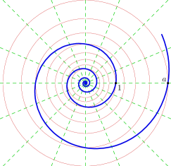
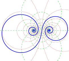
Figure 3. Logarithmic spirals (left) and loxodrome (right) with associated pencils of cycles. This is a combination of Figs. 1 and 2.

In essence, the previous proposition says that a three-cycle and $(\lambda,M)$ parametrisations are equivalent and delivers an explicit procedure producing one from another. However, three-cycle parametrisation is more geometric, since it links a loxodrome to a pair of orthogonal pencils, see Fig. 3. Furthermore, cycles $C_{1}$, $C_{2}$, $C_{3}$ (unlike parameters $\lambda$ and $M$) can be directly drawn on the plane to represent a loxodrome, which may be even omitted.

5. Applications of Three-Cycle Parametrisation

Now we present some examples of the usage of three-cycle parametrisation of loxodromes. First, we want to resolve non-uniqueness in such parametrisations. Recall, that a triple $\{C_{1},C_{2},C_{3}\}$ is non-degenerate if $C_{2}\neq C_{3}$ and $C_{3}$ is not zero-radius.

Proposition 17.

Two non-degenerate triples $\{C_{1},C_{2},C_{3}\}$ and $\{C_{1}^{\prime},C_{2}^{\prime},C_{3}^{\prime}\}$ parameterise the same loxodrome if and only if all the following conditions are satisfied:

1. Pairs $\{C_{2},C_{3}\}$ and $\{C_{2}^{\prime},C_{3}^{\prime}\}$ span the same hyperbolic pencil. That is cycles $C_{2}^{\prime}$ and $C_{3}^{\prime}$ are linear combinations of $C_{2}$ and $C_{3}$ and vise versa.

2. Pairs $\{C_{2},C_{3}\}$ and $\{C_{2}^{\prime},C_{3}^{\prime}\}$ define the same parameter $\tilde{\lambda}$:

   (16) $$\left[C_{2},C_{3}\right]=\left[C_{2}^{\prime},C_{3}^{\prime}\right].$$

3. The elliptic-hyperbolic identity holds:

   (17) $$\frac{\operatorname{arccosh}\left[C_{j},C_{j}^{\prime}\right]}{\operatorname{arccosh}\left[C_{2},C_{3}\right]}\equiv\frac{1}{2\pi}\arccos\left[C_{1},C_{1}^{\prime}\right]\pmod{1}\,,$$

   where $j$ is either $2$ or $3$.

Proof.

Necessity of (1) is obvious, since hyperbolic pencils spanned by $\{C_{2},C_{3}\}$ and $\{C_{2}^{\prime},C_{3}^{\prime}\}$ shall be both the image of concentric circles centred at origin under FLT $M$ defining the loxodrome. Necessity of (2) is also obvious since $\tilde{\lambda}$ is uniquely defined by the loxodrome. Necessity of (3) follows from the analysis of the following demonstration of sufficiency.

For sufficiency, let $M$ be FLT constructed through Procedure 15 from $\{C_{1},C_{2},C_{3}\}$. Then (1) implies that $M(C_{2}^{\prime})$ and $M(C_{3}^{\prime})$ are also circles centred at origin. Then Lem. 12 implies that the transformation $D_{x+\mathrm{i}y}(1)$, where $x=\operatorname{arccosh}\left[C_{2},C_{2}^{\prime}\right]$ and $y=\arccos\left[C_{1},C_{1}^{\prime}\right]$ maps $C_{1}^{\prime}$ and $C_{2}^{\prime}$ to $C_{1}$ and $C_{2}$ respectively. Furthermore, from identity (16) follows that the same $D_{x+\mathrm{i}y}(1)$ maps $C_{3}^{\prime}$ to $C_{3}$. Finally, condition (17) means that $x+\mathrm{i}(y+2\pi n)=a(\tilde{\lambda}+2\pi\mathrm{i})$ for $a=x/\tilde{\lambda}$ and some $n\in\mathbb{Z}{}$. In other words $D_{x+\mathrm{i}y}(1)=D_{\tilde{\lambda}}(a)$, thus $D_{x+\mathrm{i}y}(1)$ maps SLS with the parameter $\tilde{\lambda}$ to itself. Since $\{M(C_{1}),M(C_{2}),M(C_{3})\}$ and $\{M(C_{1}^{\prime}),M(C_{2}^{\prime}),M(C_{3}^{\prime})\}$ are two three-cycle parametrisations of the same SLS, $\{C_{1},C_{2},C_{3}\}$ and $\{C_{1}^{\prime},C_{2}^{\prime},C_{3}^{\prime}\}$ are two three-cycle parametrisations of the same loxodrome. ∎

See Fig. 4 for an animated family of equivalent three-cycle parametrisations of the same loxodrome (also posted at [Kisil16a]). Relation (17), which correlates elliptic and hyperbolic rotations for loxodrome, regularly appears in this context. The next topic provides another illustration of this.

Procedure 18.

To verify whether a loxodrome parametrised by three cycles $\{C_{1},C_{2},C_{3}\}$ passes a point parametrised by a zero-radius cycle $C_{0}$ we perform the following steps:

1. Define the cycle

   (18) $$C_{h}=tC_{2}+(1-t)C_{3}\,,\qquad\text{where }t=-\frac{\left\langle C_{0},C_{3}\right\rangle}{\left\langle C_{0},C_{2}-C_{3}\right\rangle}\,,$$

   which belongs to the hyperbolic pencil spanned by $\{C_{2},C_{3}\}$ and is orthogonal to $C_{0}$, that is, passes the respective point.

2. Find cycle $C_{e}$ from the elliptic pencil orthogonal to $\{C_{2},C_{3}\}$ which passes $C_{0}$. $C_{e}$ is the solution of the system of three linear (with respect to parameters of $C_{e}$) equations, cf. Ex 2:

   $$\left\langle C_{e},C_{0}\right\rangle =0\,,$$

   $$\left\langle C_{e},C_{2}\right\rangle =0\,,$$

   $$\left\langle C_{e},C_{3}\right\rangle =0\,.$$

3. Verify the elliptic-hyperbolic relation:

   (19) $$\frac{\operatorname{arccosh}\left[C_{h},C_{2}\right]}{\operatorname{arccosh}\left[C_{2},C_{3}\right]}\equiv\frac{1}{2\pi}\arccos\left[C_{e},C_{1}\right]\pmod{1}\,.$$

Proof.

Let $M$ be the standard FLT associated to $\{C_{1},C_{2},C_{3}\}$ from Procedure 15. The point $C_{0}$ belongs to the loxodrome if the transformation $D_{\tilde{\lambda}}(t)$ for some $t$ moves $M(C_{0})$ to the intersection $M(C_{1})\cap M(C_{2})$. But $D_{x+\mathrm{i}y}(1)$ with $x=\operatorname{arccosh}\left[C_{h},C_{2}\right]$ and $y=\arccos\left[C_{e},C_{1}\right]$ maps $M(C_{h})\rightarrow M(C_{2})$ and $M(C_{e})\rightarrow M(C_{1})$, thus it also maps $M(C_{0})\subset M(C_{h})\cap M(C_{e})$ to $M(C_{1})\cap M(C_{2})$. Condition (19) guaranties that $D_{x+\mathrm{i}y}(1)=D_{\tilde{\lambda}}(x/\tilde{\lambda})$, as in the previous Prop. ∎

Our final example considers two loxodromes which may have completely different associated pencils.

Procedure 19.

Let two loxodromes are parametrised by $\{C_{1},C_{2},C_{3}\}$ and $\{C_{1}^{\prime},C_{2}^{\prime},C_{3}^{\prime}\}$. Assume they intersect at some point parametrised by a zero-radius cycle $C_{0}$ (this can be checked by Procedure 18, if needed). To find the angle of intersection we perform the following steps:

1. Use (18) to find cycles $C_{h}$ and $C_{h}^{\prime}$ belonging to hyperbolic pencils, spanned by $\{C_{2},C_{3}\}$ and $\{C_{2}^{\prime},C_{3}^{\prime}\}$ respectively, and both passing $C_{0}$.

2. The intersection angle is

   (20) $$\arccos\left[C_{h},C_{h}^{\prime}\right]-\arctan\left(\frac{\tilde{\lambda}}{2\pi}\right)+\arctan\left(\frac{\tilde{\lambda}^{\prime}}{2\pi}\right)\,,$$

   where $\tilde{\lambda}$ and $\tilde{\lambda}^{\prime}$ are determined by (15).

Proof.

A loxodrome intersects any cycle from its hyperbolic pencil with the fixed angle $\arctan(\tilde{\lambda}/(2\pi))$. This is used to amend the intersection angle $\arccos\left[C_{h},C_{h}^{\prime}\right]$ of cycles from the respective hyperbolic pencils. ∎

Corollary 20.

Let a loxodrome parametrised by $\{C_{1},C_{2},C_{3}\}$ passes a point parametrised by a zero-radius cycle $C_{0}$ as in Procedure 18. A non-zero radius cycle $C$ is tangent to the loxodrome at $C_{0}$ if and only if two conditions holds:

(21) $$\begin{split}\left\langle C,C_{0}\right\rangle&=0\,,\\ \arccos\left[C,C_{h}\right]&=\arctan\left(\frac{\tilde{\lambda}}{2\pi}\right)\,,\end{split}$$

where $C_{h}$ is given by (18) and is $\tilde{\lambda}$ is determined by (15).

Proof.

The first condition simply verifies that $C$ passes $C_{0}$, cf. Ex 2. Cycle $C$, as a degenerated loxodrome, is parametrised by $\{C_{e},C,C\}$, where $C_{e}$ is any cycle orthogonal to $C$ and $C_{e}$ is not relevant in the following. The hyperbolic pencil spanned by two copies of $C$ consists of $C$ only. Thus we put $C_{h}^{\prime}=C$, $\tilde{\lambda}^{\prime}=0$ in (20) and equate it to $0$ to obtain the second identity in (21). ∎

6. Discussion and Open Questions

It was mentioned at the end of Section 4 that a three-cycle parametrisation of loxodromes is more geometrical than their presentation by a pair $(\lambda,M)$. Furthermore, three-cycle parametrisation reveals the natural analogy between elliptic and hyperbolic features of loxodromes, see (17) as an illustration. Examples in Section 5 show that various geometrical questions are explicitly answered in term of three-cycle parametrisation. Thus, our work extends the set of objects in Lie sphere geometry—circle, lines and points—to the natural maximal conformally-invariant family, which also includes loxodromes. In practical terms, three-cycle parametrisation allows to extend the library figure for Möbuis invariant geometry [Kisil14b] to operate with loxodromes as well.

It is even more important, that the presented technique is another implementation of a general framework [Kisil15a, Kisil14b], which provides a significant advance in Lie sphere geometry. The Poincaré extension of FLT from the real line to the upper half-plane was performed by a pair of orthogonal cycles in [Kisil15a]. A similar extension of FLT from the complex plane to the upper half-space can be done by a triple of pairwise orthogonal cycles. Thus, triples satisfying FLT-invariant properties (1a) and (1b) of Prop. 14 present another non-equivalent class of cycle ensembles in the sense of [Kisil15a]. In general, Lie sphere geometry can be enriched by consideration of cycle ensembles interrelated by a list of FLT-invariant properties [Kisil15a]. Such ensembles become new objects in the extended Lie spheres geometry and can be represented by points in a cycle ensemble space.

There are several natural directions to extend this work further, here are just few of them:

1. Link our “global” parametrisation of loxodromes with differential geometry approach from [Bolt07a, Porter93a, Porter07a]. Our last Cor. 20 can be a first step in this direction.

2. Consider all FLT-invariant non-equivalent classes of three-cycle ensembles on $\mathbb{C}{}$: pairwise orthogonal triples (representing points in the upper half-space [Kisil15a]), triples satisfying properties (1a) and (1b) of Prop. 14 (representing loxodromes), etc.

3. Extend this consideration for quaternions or Clifford algebras [GuerlebeckHabetaSproessig08, MoraisGeorgievSprossig14a]. The previous works [Porter98a, Porter98b] and availability of FSCc in this setup [Cnops02a]*Ch. 4 [FillmoreSpringer90a] make it rather promising.

4. Consider Möbius transformations in rings of dual and double numbers [Kisil12a, Kisil05a, Kisil15a, Kisil07a, Kisil09e, Kisil11a, Mustafa17a, BarrettBolt10a]. There are enough indications that the story will not be quite the same as for complex numbers.

5. Explore further connections of loxodromes with

   • Carleson curves and microlocal properties of singular integral operators [BishopBoettcherKarlovichSpitkovsky99a, BoettcherKarlovich01a, BarrettBolt08a]; or

   • applications in operator theory [Simon11a, Vasilevski08a].

Some combinations of those topics shall be fruitful as well.