Channel Diagonalization for Cloud Radio Access

Abstract

The diagonalization of a conventional multiple-input multiple-output (MIMO) channel into parallel and independent subchannels via singular value decomposition (SVD) is a fundamental strategy that allows the MIMO channel capacity to be achieved using scalar channel codes. This letter establishes a similar channel diagonalization result for the uplink and the downlink of a cloud radio access network (C-RAN), in which a central processor (CP) is connected to a remote radio head (RRH) serving a single user via rate-limit digital fronthaul carrying the compressed baseband signal. Specifically, we show that the diagonalization of the MIMO channel between the RRH and the user via SVD and the subsequent independent and parallel quantization of scalar signals and channel coding in each of the subchannels is optimal. This letter establishes this fact using the majorization theory. Further, an uplink-downlink duality for the multiple-antenna C-RAN is identified for this single-user case.

I Introduction

A fundamental result in multiple-input multiple-output (MIMO) communication is that the diagonalization of a Gaussian vector channel $\mbox{\boldmath{$y$}}=\mbox{\boldmath{$H$}}\mbox{\boldmath{$x$}}+\mbox{\boldmath{$z$}}$ via singular value decomposition (SVD), $\mbox{\boldmath{$H$}}=\mbox{\boldmath{$U$}}_{H}\mbox{\boldmath{$\Lambda$}}_{H}\mbox{\boldmath{$V$}}_{H}^{H}$, leads to an optimal transmission and reception strategy. The use of the singular vectors $\mbox{\boldmath{$V$}}_{H}$ as the precoders, the singular vectors $\mbox{\boldmath{$U$}}_{H}$ as the receive beamformers, and the use of error-correcting codes designed for single-input single-output (SISO) additive white Gaussian noise (AWGN) channel over the independent and parallel subchannels can achieve the capacity of the overall Gaussian vector channel [1]. Moreover, if the uplink and downlink channels are reciprocals of each other, because the singular values of $H$ and $\mbox{\boldmath{$H$}}^{H}$ are the same, the capacities of the uplink and downlink channels are also the same.

This letter investigates the uplink and downlink of a cloud radio-access network (C-RAN) [2] consisting of a cloud-based central processor (CP), a remote radio head (RRH), and one user. The RRH is connected to the CP via a finite-capacity digital link. In the uplink, the RRH compresses the received baseband analog signal and sends the compressed signal to the CP for demodulation and decoding. In the downlink, the CP pre-computes the desired analog transmit signal and sends a compressed version to the RRH for transmission. For such a C-RAN, we ask the question of whether the natural strategy of first diagonalizing the MIMO channel into parallel scalar channels followed by independently compressing the scalar signal and coding over each of the subchannels is optimal.

This letter answers the question in the affirmative by utilizing the majorization theory [3]. The answer is nontrivial because it involves a joint optimization of transmission and quantization under finite fronthaul. As a consequence of the optimality of channel diagonalization, an uplink-downlink duality is established for the single-RRH single-user C-RAN.

We note that although a main future benefit of C-RAN stems from multiple-RRH cooperation for interference mitigation, the single-RRH single-user C-RAN considered here is already of interest, because the processing of baseband signals in the cloud provides computational offloading benefit [4] even without RRH cooperation. This paper considers C-RAN with a single user. The single-user C-RAN model considered in this letter can also be thought of as corresponding to one subcarrier of an orthogonal frequency-division multiple-access (OFDMA) C-RAN system, in which users are separated via orthogonal subcarriers, free of co-channel interference [5].

II Uplink and Downlink C-RAN Model

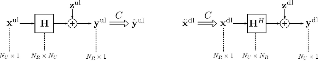
Figure 1: System models of single-user multi-antenna C-RAN in the uplink (left) and the downlink (right).

Consider the uplink and downlink C-RAN model consisting of one CP, one RRH and one user, as shown in Fig. 1. The RRH is equipped with $N_{R}>1$ antennas; the user is equipped with $N_{U}>1$ antennas. In the uplink, the channel from the user to the RRH is denoted by $\mbox{\boldmath{$H$}}\in\mathbb{C}^{N_{R}\times N_{U}}$; in the dual downlink, the channel from the RRH to the user is given by $\mbox{\boldmath{$H$}}^{H}$ by reciprocity. Without loss of generality, we assume that the rank of $H$ is $\min(N_{R},N_{U})$. The transmit power constraint is denoted by $P$ for both the uplink and the downlink. It is assumed that the RRH is connected to the CP via a (noiseless) digital fronthaul link of capacity $C$.

This letter considers compression-based strategies for relaying information between the CP and the RRH via the fronthaul link for both uplink and downlink [6, 7]. Although from a capacity perspective a RRH capable of decoding and encoding can potentially outperform compression in our setting, the compression strategy significantly simplifies the computational requirements at the RRH. For this reason, the practical implementations of C-RAN in 5G cellular systems are likely to involve compression over the fronthaul [4].

II-A Uplink C-RAN

The uplink discrete-time baseband channel is modeled as

$$\mbox{\boldmath{$y$}}^{\rm ul}=\mbox{\boldmath{$H$}}\mbox{\boldmath{$x$}}^{\rm ul}+\mbox{\boldmath{$z$}}^{\rm ul},$$ (1)

where it is assumed that the user transmits a Gaussian signal with covariance $\mbox{\boldmath{$S$}}^{\rm ul}$, i.e., $\mbox{\boldmath{$x$}}^{\rm ul}\sim\mathcal{CN}(\mbox{\boldmath{$0$}},\mbox{\boldmath{$S$}}^{\rm ul})$, and $\mbox{\boldmath{$z$}}^{\rm ul}\sim\mathcal{CN}(\mbox{\boldmath{$0$}},\sigma^{2}\mbox{\boldmath{$I$}})$ denotes the noise at the RRH. The total transmit power of the user across all the antennas is ${\rm tr}(\mbox{\boldmath{$S$}}^{\rm ul})$. The RRH compresses its received signal and sends the compressed signal to the CP. This quantization process can be modeled as

$$\tilde{\mbox{\boldmath{$y$}}}^{\rm ul}=\mbox{\boldmath{$y$}}^{\rm ul}+\mbox{\boldmath{$e$}}^{\rm ul},$$ (2)

where it is assumed that the quantization noise has a Gaussian distribution with covariance $\mbox{\boldmath{$Q$}}^{\rm ul}$, i.e., $\mbox{\boldmath{$e$}}^{\rm ul}\sim\mathcal{CN}(\mbox{\boldmath{$0$}},\mbox{\boldmath{$Q$}}^{\rm ul})$. Based on the rate-distortion theory [8], the fronthaul rate needed for transmitting $\tilde{\mbox{\boldmath{$y$}}}^{\rm ul}$ can be expressed as

$$I(\mbox{\boldmath{$y$}}^{\rm ul};\tilde{\mbox{\boldmath{$y$}}}^{\rm ul})=\log_{2}\frac{\left|\mbox{\boldmath{$H$}}\mbox{\boldmath{$S$}}^{\rm ul}\mbox{\boldmath{$H$}}^{H}+\mbox{\boldmath{$Q$}}^{\rm ul}+\sigma^{2}\mbox{\boldmath{$I$}}\right|}{\left|\mbox{\boldmath{$Q$}}^{\rm ul}\right|}.$$ (3)

The achievable rate for the user, accounting for the quantization noise, can now be expressed as

$$I(\mbox{\boldmath{$x$}}^{\rm ul};\tilde{\mbox{\boldmath{$y$}}}^{\rm ul})=\log_{2}\frac{\left|\mbox{\boldmath{$H$}}\mbox{\boldmath{$S$}}^{\rm ul}\mbox{\boldmath{$H$}}^{H}+\mbox{\boldmath{$Q$}}^{\rm ul}+\sigma^{2}\mbox{\boldmath{$I$}}\right|}{\left|\mbox{\boldmath{$Q$}}^{\rm ul}+\sigma^{2}\mbox{\boldmath{$I$}}\right|}.$$ (4)

With a transmit power constraint $P$ and fronthaul constraint $C$, the maximum achievable uplink rate for the user is the optimal value of the following optimization problem [6]:

$$\mathrm{(P1)}:~{}\mathop{\mathrm{maximize}}_{\mbox{\boldmath{$S$}}^{\rm ul},\mbox{\boldmath{$Q$}}^{\rm ul}} ~{}~{}~{}\log_{2}\frac{\left|\mbox{\boldmath{$H$}}\mbox{\boldmath{$S$}}^{\rm ul}\mbox{\boldmath{$H$}}^{H}+\mbox{\boldmath{$Q$}}^{\rm ul}+\sigma^{2}\mbox{\boldmath{$I$}}\right|}{\left|\mbox{\boldmath{$Q$}}^{\rm ul}+\sigma^{2}\mbox{\boldmath{$I$}}\right|}$$

$$\mathrm{subject\ to} ~{}~{}~{}\log_{2}\frac{\left|\mbox{\boldmath{$H$}}\mbox{\boldmath{$S$}}^{\rm ul}\mbox{\boldmath{$H$}}^{H}+\mbox{\boldmath{$Q$}}^{\rm ul}+\sigma^{2}\mbox{\boldmath{$I$}}\right|}{\left|\mbox{\boldmath{$Q$}}^{\rm ul}\right|}\leq C,$$

$$~{}~{}~{}{\rm tr}\left(\mbox{\boldmath{$S$}}^{\rm ul}\right)\leq P.$$

II-B Downlink C-RAN

The downlink discrete-time baseband channel is modeled as

$$\mbox{\boldmath{$y$}}^{\rm dl}=\mbox{\boldmath{$H$}}^{H}\mbox{\boldmath{$x$}}^{\rm dl}+\mbox{\boldmath{$z$}}^{\rm dl},$$ (5)

where $\mbox{\boldmath{$x$}}^{\rm dl}$ denotes the transmit signal of the RRH, and $\mbox{\boldmath{$z$}}^{\rm dl}\sim\mathcal{CN}(\mbox{\boldmath{$0$}},\sigma^{2}\mbox{\boldmath{$I$}})$ denotes the AWGN at the user.

The transmit signal $\mbox{\boldmath{$x$}}^{\rm dl}$ is a compressed version of the beamformed signal, assumed to be Gaussian distributed as $\tilde{\mbox{\boldmath{$x$}}}^{\rm dl}\sim\mathcal{CN}(\mbox{\boldmath{$0$}},\tilde{\mbox{\boldmath{$S$}}}^{\rm dl})$. The compression process is modeled as

$$\mbox{\boldmath{$x$}}^{\rm dl}=\tilde{\mbox{\boldmath{$x$}}}^{\rm dl}+\mbox{\boldmath{$e$}}^{\rm dl},$$ (6)

where the compression noise is also assumed to be Gaussian, i.e., $\mbox{\boldmath{$e$}}^{\rm dl}\sim\mathcal{CN}(\mbox{\boldmath{$0$}},\mbox{\boldmath{$Q$}}^{\rm dl})$. The total transmit power of the RRH across all the antennas can now be expressed as ${\rm tr}(\tilde{\mbox{\boldmath{$S$}}}^{\rm dl}+\mbox{\boldmath{$Q$}}^{\rm dl})$. By rate-distortion theory, the fronthaul rate for transmitting $\tilde{\mbox{\boldmath{$x$}}}^{\rm dl}$ can be expressed as

$$I(\tilde{\mbox{\boldmath{$x$}}}^{\rm dl};\mbox{\boldmath{$x$}}^{\rm dl})=\log_{2}\frac{|\tilde{\mbox{\boldmath{$S$}}}^{\rm dl}+\mbox{\boldmath{$Q$}}^{\rm dl}|}{\left|\mbox{\boldmath{$Q$}}^{\rm dl}\right|}.$$ (7)

The achievable rate of the user is

$$I(\tilde{\mbox{\boldmath{$x$}}}^{\rm dl};\mbox{\boldmath{$y$}}^{\rm dl})=\log_{2}\frac{\left|\mbox{\boldmath{$H$}}^{H}\tilde{\mbox{\boldmath{$S$}}}^{\rm dl}\mbox{\boldmath{$H$}}+\mbox{\boldmath{$H$}}^{H}\mbox{\boldmath{$Q$}}^{\rm dl}\mbox{\boldmath{$H$}}+\sigma^{2}\mbox{\boldmath{$I$}}\right|}{\left|\mbox{\boldmath{$H$}}^{H}\mbox{\boldmath{$Q$}}^{\rm dl}\mbox{\boldmath{$H$}}+\sigma^{2}\mbox{\boldmath{$I$}}\right|}.$$ (8)

With the same transmit power constraint $P$ and fronthaul constraint $C$ as in the uplink, the maximum achievable downlink rate for the user is the optimal value of the following optimization problem [7]:

$$\mathrm{(P2)}:~{}\mathop{\mathrm{maximize}}_{\tilde{\mbox{\boldmath{$S$}}}^{\rm dl},\mbox{\boldmath{$Q$}}^{\rm dl}} ~{}~{}~{}\log_{2}\frac{\left|\mbox{\boldmath{$H$}}^{H}\tilde{\mbox{\boldmath{$S$}}}^{\rm dl}\mbox{\boldmath{$H$}}+\mbox{\boldmath{$H$}}^{H}\mbox{\boldmath{$Q$}}^{\rm dl}\mbox{\boldmath{$H$}}+\sigma^{2}\mbox{\boldmath{$I$}}\right|}{\left|\mbox{\boldmath{$H$}}^{H}\mbox{\boldmath{$Q$}}^{\rm dl}\mbox{\boldmath{$H$}}+\sigma^{2}\mbox{\boldmath{$I$}}\right|}$$

$$\mathrm{subject\ to} ~{}~{}~{}\log_{2}\frac{|\tilde{\mbox{\boldmath{$S$}}}^{\rm dl}+\mbox{\boldmath{$Q$}}^{\rm dl}|}{\left|\mbox{\boldmath{$Q$}}^{\rm dl}\right|}\leq C,$$

$$~{}~{}~{}{\rm tr}\left(\tilde{\mbox{\boldmath{$S$}}}^{\rm dl}+\mbox{\boldmath{$Q$}}^{\rm dl}\right)\leq P.$$

III Optimality of Channel Diagonalization

This letter shows that the SVD diagonalization of the channel is optimal for both the uplink and the downlink C-RAN by providing optimal solutions to problems (P1) and (P2). Define the SVD of $H$ as $\mbox{\boldmath{$H$}}=\mbox{\boldmath{$U$}}_{H}\mbox{\boldmath{$\Lambda$}}_{H}\mbox{\boldmath{$V$}}_{H}^{H}$, where $\mbox{\boldmath{$\Lambda$}}_{H}\in\mathbb{C}^{N_{R}\times N_{U}}$ is a rectangular diagonal matrix with $D={\rm rank}(\mbox{\boldmath{$H$}})=\min(N_{R},N_{U})$ diagonal elements denoted by $h_{1},\cdots,h_{D}$, with $|h_{1}|\geq\cdots\geq|h_{D}|$, and $\mbox{\boldmath{$U$}}_{H}\in\mathbb{C}^{N_{R}\times N_{R}}$ and $\mbox{\boldmath{$V$}}_{H}\in\mathbb{C}^{N_{U}\times N_{U}}$ are unitary matrices.

Theorem 1

The optimal solution to problem (P1) has the following form:

$$\mbox{\boldmath{$S$}}^{\ast,\rm ul}=\mbox{\boldmath{$V$}}_{H}\mbox{\boldmath{$\Lambda$}}_{S^{\rm ul}}\mbox{\boldmath{$V$}}_{H}^{H},$$ (9)

$$\mbox{\boldmath{$Q$}}^{\ast,\rm ul}=\mbox{\boldmath{$U$}}_{H}\mbox{\boldmath{$\Lambda$}}_{Q^{\rm ul}}\mbox{\boldmath{$U$}}_{H}^{H},$$ (10)

where $\mbox{\boldmath{$\Lambda$}}_{S^{\rm ul}}={\rm diag}(p^{\rm ul}_{1},\cdots,p^{\rm ul}_{N_{U}})$ and $\mbox{\boldmath{$\Lambda$}}_{Q^{\rm ul}}={\rm diag}(q^{\rm ul}_{1},\cdots,q^{\rm ul}_{N_{R}})$ are diagonal matrices with non-negative diagonal elements $p^{\rm ul}_{1},\cdots,p^{\rm ul}_{N_{U}}$ and $q^{\rm ul}_{1},\cdots,q^{\rm ul}_{N_{R}}$.

Theorem 2

The optimal solution to problem (P2) has the following form:

$$\tilde{\mbox{\boldmath{$S$}}}^{\ast,\rm dl}=\mbox{\boldmath{$U$}}_{H}\mbox{\boldmath{$\Lambda$}}_{\tilde{S}^{\rm dl}}\mbox{\boldmath{$U$}}_{H}^{H},$$ (11)

$$\mbox{\boldmath{$Q$}}^{\ast,\rm dl}=\mbox{\boldmath{$U$}}_{H}\mbox{\boldmath{$\Lambda$}}_{Q^{\rm dl}}\mbox{\boldmath{$U$}}_{H}^{H},$$ (12)

where $\mbox{\boldmath{$\Lambda$}}_{\tilde{S}^{\rm dl}}={\rm diag}(\tilde{p}^{\rm dl}_{1},\cdots,\tilde{p}^{\rm dl}_{N_{R}})$ and $\mbox{\boldmath{$\Lambda$}}_{Q^{\rm dl}}={\rm diag}(q^{\rm dl}_{1},\cdots,q^{\rm dl}_{N_{R}})$ are diagonal matrices with non-negative diagonal elements $\tilde{p}^{\rm dl}_{1},\cdots,\tilde{p}^{\rm dl}_{N_{R}}$ and $q^{\rm dl}_{1},\cdots,q^{\rm dl}_{N_{R}}$.

It is well-known that to maximize the capacity of the vector point-to-point channel, the optimal strategy is to set the precoder and receiver beamformer as singular vectors in $\mbox{\boldmath{$V$}}_{H}$ and $\mbox{\boldmath{$U$}}_{H}$ so as to diagonalize the channel $H$ [1]. Theorems 1 and 2 imply that under the assumption of compression-based strategies for C-RAN, the optimal transmit and receive scheme is also to diagonalize the vector channel into $D={\rm rank}(\mbox{\boldmath{$H$}})$ parallel sub-channels such that a simple quantization of scalars together with scalar AWGN codes on each subchannel is optimal. The proofs are based on majorization theory [3] and are deferred to the next section. Here, $h_{d}$, $(p^{\rm ul}_{d},\tilde{p}^{\rm dl}_{d}+q^{\rm dl}_{d})$, and $(q^{\rm ul}_{d},q^{\rm dl}_{d})$ are the channel strength, transmit power, and quantization noise level of the uplink/downlink subchannel $d$.

The optimality of channel diagonalization allows us to establish an uplink-downlink duality relationship for the multi-antenna single-user single-RRH C-RAN. Based on Theorems 1 and 2, the maximizations of the uplink and downlink rates for C-RAN, i.e., (P1) and (P2), reduce to the following scalar optimization problems. For the uplink, we have:

$$~{}\mathop{\mathrm{maximize}}_{\{p^{\rm ul}_{d},q^{\rm ul}_{d}\}} ~{}~{}~{}\sum\limits_{d=1}^{D}\log_{2}\left(1+\frac{|h_{d}|^{2}p^{\rm ul}_{d}}{q^{\rm ul}_{d}+\sigma^{2}}\right)$$ (13)

$$\mathrm{subject\ to} ~{}~{}~{}\sum\limits_{d=1}^{D}\log_{2}\left(\frac{|h_{d}|^{2}p^{\rm ul}_{d}+q^{\rm ul}_{d}+\sigma^{2}}{q^{\rm ul}_{d}}\right)\leq C,$$

$$~{}~{}~{}\sum\limits_{d=1}^{D}p^{\rm ul}_{d}\leq P,$$

and for the downlink, we have:

$$~{}\mathop{\mathrm{maximize}}_{\{\tilde{p}^{\rm dl}_{d},q^{\rm dl}_{d}\}} ~{}~{}~{}\sum\limits_{d=1}^{D}\log_{2}\left(1+\frac{|h_{d}|^{2}\tilde{p}^{\rm dl}_{d}}{|h_{d}|^{2}q^{\rm dl}_{d}+\sigma^{2}}\right)$$ (14)

$$\mathrm{subject\ to} ~{}~{}~{}\sum\limits_{d=1}^{D}\log_{2}\left(\frac{\tilde{p}^{\rm dl}_{d}+q^{\rm dl}_{d}}{q^{\rm dl}_{d}}\right)\leq C,$$

$$~{}~{}~{}\sum\limits_{d=1}^{D}(\tilde{p}^{\rm dl}_{d}+q^{\rm dl}_{d})\leq P.$$

Although the above problems (13) and (14) are not convex, there is an interesting duality between the two. For the SISO C-RAN, the duality has been shown in [9, Theorem 1]. Specifically, consider the case of $D=1$, the maximum uplink achievable rate is

$$\log_{2}\left(1+\frac{|h|^{2}p^{\rm ul}}{q^{\rm ul}+\sigma^{2}}\right)=\log_{2}\left(\frac{|h|^{2}P+\sigma^{2}}{\sigma^{2}+2^{-C}|h|^{2}P}\right),$$ (15)

where we have used the relationships $p^{\rm ul}=P$ and

$$\log_{2}\left(\frac{|h|^{2}p^{\rm ul}+q^{\rm ul}+\sigma^{2}}{q^{\rm ul}}\right)=C.$$ (16)

Likewise in the downlink $D=1$ case, utilizing the relationships $\tilde{p}^{\rm dl}+q^{\rm dl}=P$ and

$$\log_{2}\left(\frac{\tilde{p}^{\rm dl}+q^{\rm dl}}{q^{\rm dl}}\right)=C,$$ (17)

it can be shown that the maximum downlink achievable rate is exactly the same as the uplink:

$$\log_{2}\left(1+\frac{|h|^{2}\tilde{p}^{\rm dl}}{|h|^{2}q^{\rm dl}+\sigma^{2}}\right)=\log_{2}\left(\frac{|h|^{2}P+\sigma^{2}}{\sigma^{2}+2^{-C}|h|^{2}P}\right).$$ (18)

By applying this result to each subchannel $d$, it can be shown that the optimal value of the problem (13) must be the same as that of the problem (14).

Theorem 3

Consider a C-RAN model implementing compression-based strategies in both the uplink and the downlink, where both the user and RRH are equipped with multiple antennas. Any rate that is achievable in the uplink is achievable with the same sum-power and fronthaul capacity constraint in the downlink, and vice versa.

The above result can be thought of as a generalization of celebrated uplink-downlink duality (e.g. [10]) to the C-RAN, but restricted to the single-RRH single-user case.

IV Proofs via Logarithmic Majorization

IV-A Proof of Theorem 1

First by [11, Theorem 2], we can recast problem (P1) as

$$\mathop{\mathrm{maximize}}_{R,{\mathbf{S}}^{\rm ul},{\mathbf{Q}}^{\rm ul}} ~{}~{}~{}R$$ (19)

$$\mathrm{subject\ to} ~{}~{}~{}R\leq\log_{2}\left|\mbox{\boldmath{$I$}}+\mbox{\boldmath{$H$}}\mbox{\boldmath{$S$}}^{\rm ul}\mbox{\boldmath{$H$}}^{H}(\mbox{\boldmath{$Q$}}^{\rm ul}+\sigma^{2}\mbox{\boldmath{$I$}})^{-1}\right|,$$

$$~{}~{}~{}R+\log_{2}\frac{\left|\mbox{\boldmath{$Q$}}^{\rm ul}+\sigma^{2}\mbox{\boldmath{$I$}}\right|}{\left|\mbox{\boldmath{$Q$}}^{\rm ul}\right|}\leq C,$$

$$~{}~{}~{}{\rm tr}\left(\mbox{\boldmath{$S$}}^{\rm ul}\right)\leq P.$$

Define the SVD of $\mbox{\boldmath{$\Phi$}}=\mbox{\boldmath{$H$}}\mbox{\boldmath{$S$}}^{\rm ul}\mbox{\boldmath{$H$}}^{H}$ and $\mbox{\boldmath{$Q$}}^{\rm ul}$ as $\mbox{\boldmath{$\Phi$}}=\mbox{\boldmath{$U$}}_{\Phi}\mbox{\boldmath{$\Lambda$}}_{\Phi}\mbox{\boldmath{$U$}}_{\Phi}^{H}$ and $\mbox{\boldmath{$Q$}}^{\rm ul}=\mbox{\boldmath{$U$}}_{Q^{\rm ul}}\mbox{\boldmath{$\Lambda$}}_{Q^{\rm ul}}\mbox{\boldmath{$U$}}_{Q^{\rm ul}}^{H}$, respectively, for some $\mbox{\boldmath{$\Lambda$}}_{\Phi}={\rm diag}(\lambda_{\Phi,1},\cdots,\lambda_{\Phi,N_{R}})$ with $\lambda_{\Phi,1}\geq\cdots\geq\lambda_{\Phi,N_{R}}$, and $\mbox{\boldmath{$\Lambda$}}_{Q^{\rm ul}}={\rm diag}(\lambda_{U^{\rm ul},1},\cdots,\lambda_{U^{\rm ul},N_{R}})$ with $\lambda_{U^{\rm ul},1}\leq\cdots\leq\lambda_{U^{\rm ul},N_{R}}$. Note that the optimization variables of problem (19) are changed to $R$, $\Phi$ (instead of $\mbox{\boldmath{$S$}}^{\rm ul}$), and $\mbox{\boldmath{$Q$}}^{\rm ul}$.

Consider the first constraint in problem (19). Given any matrix $A$, define $\mbox{\boldmath{$\gamma$}}^{\downarrow}(\mbox{\boldmath{$A$}})$ and $\mbox{\boldmath{$\gamma$}}^{\uparrow}(\mbox{\boldmath{$A$}})$ as the vectors consisting of all the eigenvalues of $A$ in decreasing and increasing order, respectively. According to [3, 9.H.1.d], $\mbox{\boldmath{$\gamma$}}(\mbox{\boldmath{$\Phi$}}(\mbox{\boldmath{$Q$}}^{\rm ul}+\sigma^{2}\mbox{\boldmath{$I$}})^{-1})$ is logarithmically majorized by $\mbox{\boldmath{$\gamma$}}^{\downarrow}(\mbox{\boldmath{$\Phi$}})\circ\mbox{\boldmath{$\gamma$}}^{\downarrow}((\mbox{\boldmath{$Q$}}^{\rm ul}+\sigma^{2}\mbox{\boldmath{$I$}})^{-1})$ (see [12, Definition 1.4]), where $\circ$ represents the elementwise product. Moreover, it can be shown that $f(\mbox{\boldmath{$x$}})=\sum_{n=1}^{N}\log_{2}(\sigma^{2}+x_{n})$ is a Schur-geometrically-convex function of $\mbox{\boldmath{$x$}}=[x_{1},\cdots,x_{N}]^{T}$ (see [12, Definition 1.5]). Since the diagonal elements of $\mbox{\boldmath{$\Lambda$}}_{\Phi}$, $(\mbox{\boldmath{$\Lambda$}}_{Q^{\rm ul}}+\sigma^{2}\mbox{\boldmath{$I$}})^{-1}$ are all arranged in deceasing order, we thus have

$$\log_{2}\left|\mbox{\boldmath{$I$}}+\mbox{\boldmath{$H$}}\mbox{\boldmath{$S$}}^{\rm ul}\mbox{\boldmath{$H$}}^{H}(\mbox{\boldmath{$Q$}}^{\rm ul}+\sigma^{2}\mbox{\boldmath{$I$}})^{-1}\right|$$

$$= \log_{2}\left|\mbox{\boldmath{$I$}}+\mbox{\boldmath{$\Phi$}}(\mbox{\boldmath{$Q$}}^{\rm ul}+\sigma^{2}\mbox{\boldmath{$I$}})^{-1}\right|$$

$$= \log_{2}|\sigma^{2}\mbox{\boldmath{$I$}}+{\rm diag}(\mbox{\boldmath{$\gamma$}}(\mbox{\boldmath{$\Phi$}}(\mbox{\boldmath{$Q$}}^{\rm ul}+\sigma^{2}\mbox{\boldmath{$I$}})^{-1}))|$$

$$\leq \log_{2}|\sigma^{2}\mbox{\boldmath{$I$}}+{\rm diag}(\mbox{\boldmath{$\gamma$}}^{\downarrow}(\mbox{\boldmath{$\Phi$}})\circ\mbox{\boldmath{$\gamma$}}^{\downarrow}((\mbox{\boldmath{$Q$}}^{\rm ul}+\sigma^{2}\mbox{\boldmath{$I$}})^{-1}))|$$

$$= \log_{2}|\sigma^{2}\mbox{\boldmath{$I$}}+\mbox{\boldmath{$\Lambda$}}_{\Phi}(\mbox{\boldmath{$\Lambda$}}_{Q^{\rm ul}}+\sigma^{2}\mbox{\boldmath{$I$}})^{-1}|,$$ (20)

where the equality holds if and only if $\mbox{\boldmath{$U$}}_{Q^{\rm ul}}=\mbox{\boldmath{$U$}}_{\Phi}$.

Next, consider the second constraint in problem (19). It can be observed that it does not depend on $\mbox{\boldmath{$U$}}_{\Phi}$ and $\mbox{\boldmath{$U$}}_{Q^{\rm ul}}$.

Finally, consider the third constraint in problem (19). Define the truncated SVD of $H$ as $\mbox{\boldmath{$H$}}=\bar{\mbox{\boldmath{$U$}}}_{H}\bar{\mbox{\boldmath{$\Lambda$}}}_{H}\bar{\mbox{\boldmath{$V$}}}_{H}^{H}$, where $\bar{\mbox{\boldmath{$U$}}}_{H}$ and $\bar{\mbox{\boldmath{$V$}}}_{H}$ consist of the first $D=\min(N_{R},N_{U})$ columns of $\mbox{\boldmath{$U$}}_{H}$ and $\mbox{\boldmath{$V$}}_{H}$ with $\bar{\mbox{\boldmath{$U$}}}_{H}^{H}\bar{\mbox{\boldmath{$U$}}}_{H}=\bar{\mbox{\boldmath{$V$}}}_{H}^{H}\bar{\mbox{\boldmath{$V$}}}_{H}=\mbox{\boldmath{$I$}}$, and $\bar{\mbox{\boldmath{$\Lambda$}}}_{H}\in\mathbb{C}^{D\times D}$ is the block-submatrix of $\mbox{\boldmath{$\Lambda$}}_{H}$ with indices taken from $1$ to $D$. Since $\mbox{\boldmath{$\Phi$}}=\mbox{\boldmath{$H$}}\mbox{\boldmath{$S$}}^{\rm ul}\mbox{\boldmath{$H$}}^{H}$, we have $\bar{\mbox{\boldmath{$V$}}}_{H}^{H}\mbox{\boldmath{$S$}}^{\rm ul}\bar{\mbox{\boldmath{$V$}}}_{H}=\bar{\mbox{\boldmath{$\Lambda$}}}_{H}^{-1}\bar{\mbox{\boldmath{$U$}}}_{H}^{H}\mbox{\boldmath{$\Phi$}}\bar{\mbox{\boldmath{$U$}}}_{H}\bar{\mbox{\boldmath{$\Lambda$}}}_{H}^{-1}$. It then follows that

$${\rm tr}\left(\mbox{\boldmath{$S$}}^{\rm ul}\right) \overset{(a)}{\geq}{\rm tr}(\mbox{\boldmath{$S$}}^{\rm ul}\bar{\mbox{\boldmath{$V$}}}_{H}\bar{\mbox{\boldmath{$V$}}}_{H}^{H})$$

$$={\rm tr}\left(\mbox{\boldmath{$\Phi$}}\bar{\mbox{\boldmath{$U$}}}_{H}\bar{\mbox{\boldmath{$\Lambda$}}}_{H}^{-2}\bar{\mbox{\boldmath{$U$}}}_{H}^{H}\right)$$

$$={\rm tr}\left(\mbox{\boldmath{$\Phi$}}\mbox{\boldmath{$U$}}_{H}(\mbox{\boldmath{$\Lambda$}}_{H}\mbox{\boldmath{$\Lambda$}}_{H}^{H})^{-1}\mbox{\boldmath{$U$}}_{H}^{H}\right),$$ (21)

where $(a)$ is from [10, Appendix A]. Since the diagonal elements of $(\mbox{\boldmath{$\Lambda$}}_{H}\mbox{\boldmath{$\Lambda$}}_{H}^{H})^{-1}$ are arranged in increasing order, according to [3, 9.H.1.h], we have

$${\rm tr}\left(\mbox{\boldmath{$\Phi$}}\bar{\mbox{\boldmath{$U$}}}_{H}(\mbox{\boldmath{$\Lambda$}}_{H}\mbox{\boldmath{$\Lambda$}}_{H}^{H})^{-1}\bar{\mbox{\boldmath{$U$}}}_{H}^{H}\right) \geq{\rm tr}\left(\mbox{\boldmath{$\Lambda$}}_{\Phi}(\mbox{\boldmath{$\Lambda$}}_{H}\mbox{\boldmath{$\Lambda$}}_{H}^{H})^{-1}\right)$$

$$=\sum\limits_{d=1}^{N_{R}}\frac{\lambda_{\Phi,d}}{|h_{d}|^{2}}.$$ (22)

Note that if $h_{d}=0$, for $d=D+1,\cdots,N_{R}$, we have $\lambda_{\Phi,d}=0$ and $\frac{\lambda_{\Phi,d}}{|h_{d}|^{2}}$ is understood to be zero. Combining (IV-A) and (IV-A), it follows that the transmit power is lower-bounded by $\sum_{d=1}^{N_{R}}\lambda_{\Phi,d}/|h_{d}|^{2}$. Observe that if $\mbox{\boldmath{$U$}}_{\Phi}=\mbox{\boldmath{$U$}}_{H}$, or equivalently, the SVD of $S$ is in the form of (9), the above lower bound on transmit power is achieved, i.e., ${\rm tr}(\mbox{\boldmath{$S$}}^{\rm ul})=\sum_{d=1}^{N_{R}}\lambda_{\Phi,d}/|h_{d}|^{2}$.

Further, regardless of the choice of $\mbox{\boldmath{$U$}}_{\Phi}$, the upper bound of $\log_{2}\left|\mbox{\boldmath{$I$}}+\mbox{\boldmath{$H$}}\mbox{\boldmath{$S$}}^{\rm ul}\mbox{\boldmath{$H$}}^{H}(\mbox{\boldmath{$Q$}}^{\rm ul}+\sigma^{2}\mbox{\boldmath{$I$}})^{-1}\right|$ given in (IV-A) can be achieved as long as the optimal $\mbox{\boldmath{$U$}}_{Q^{\rm ul}}$ is set to be $\mbox{\boldmath{$U$}}_{\Phi}$. As a consequence, the optimal solution is to set $\mbox{\boldmath{$U$}}_{\Phi}$ as $\mbox{\boldmath{$U$}}_{H}$, i.e., (9), since it makes the transmit power the lowest, and to set $\mbox{\boldmath{$U$}}_{Q^{\rm ul}}=\mbox{\boldmath{$U$}}_{\Phi}=\mbox{\boldmath{$U$}}_{H}$ to achieve the maximum value of $\log_{2}\left|\mbox{\boldmath{$I$}}+\mbox{\boldmath{$H$}}\mbox{\boldmath{$S$}}^{\rm ul}\mbox{\boldmath{$H$}}^{H}(\mbox{\boldmath{$Q$}}^{\rm ul}+\sigma^{2}\mbox{\boldmath{$I$}})^{-1}\right|$. This makes the feasible set of $R$, $\mbox{\boldmath{$\Lambda$}}_{S^{\rm ul}}$, and $\mbox{\boldmath{$\Lambda$}}_{Q^{\rm ul}}$ in problem (19) the largest, which results in the best objective value. Theorem 1 is thus proved.

IV-B Proof of Theorem 2

For convenience, define $\mbox{\boldmath{$S$}}^{\rm dl}=\tilde{\mbox{\boldmath{$S$}}}^{\rm dl}+\mbox{\boldmath{$Q$}}^{\rm dl}$ as the covariance matrix of the transmit signal $\mbox{\boldmath{$x$}}^{\rm dl}$. Problem (P2) reduces to:

$$\mathop{\mathrm{maximize}}_{{\mathbf{S}}^{\rm dl},{\mathbf{Q}}^{\rm dl}} ~{}~{}~{}\log_{2}\frac{\left|\mbox{\boldmath{$H$}}^{H}\mbox{\boldmath{$S$}}^{\rm dl}\mbox{\boldmath{$H$}}+\sigma^{2}\mbox{\boldmath{$I$}}\right|}{\left|\mbox{\boldmath{$H$}}^{H}\mbox{\boldmath{$Q$}}^{\rm dl}\mbox{\boldmath{$H$}}+\sigma^{2}\mbox{\boldmath{$I$}}\right|}$$ (23)

$$\mathrm{subject\ to} ~{}~{}~{}\log_{2}\frac{\left|\mbox{\boldmath{$S$}}^{\rm dl}\right|}{\left|\mbox{\boldmath{$Q$}}^{\rm dl}\right|}\leq C,$$

$$~{}~{}~{}{\rm tr}\left(\mbox{\boldmath{$S$}}^{\rm dl}\right)\leq P.$$

First, given any $\mbox{\boldmath{$Q$}}^{\rm dl}=\bar{\mbox{\boldmath{$Q$}}}^{\rm dl}$, we optimize over $\mbox{\boldmath{$S$}}^{\rm dl}$. Define the SVD of $\mbox{\boldmath{$S$}}^{\rm dl}=\mbox{\boldmath{$U$}}_{S^{\rm dl}}\mbox{\boldmath{$\Lambda$}}_{S^{\rm dl}}\mbox{\boldmath{$U$}}_{S^{\rm dl}}^{H}$, where $\mbox{\boldmath{$\Lambda$}}_{S^{\rm dl}}={\rm diag}(p^{\rm dl}_{1},\cdots,p^{\rm dl}_{N_{R}})$ with $p^{\rm dl}_{1}\geq\cdots\geq p^{\rm dl}_{N_{R}}$. Then, problem (23) reduces to the following problem:

$$\mathop{\mathrm{maximize}}_{{\mathbf{U}}_{S^{\rm dl}},{\mathbf{\Lambda}}_{S^{\rm dl}}} ~{}~{}~{}\log_{2}|\mbox{\boldmath{$U$}}_{S^{\rm dl}}\mbox{\boldmath{$\Lambda$}}_{S^{\rm dl}}\mbox{\boldmath{$U$}}_{S^{\rm dl}}^{H}\mbox{\boldmath{$U$}}_{H}\mbox{\boldmath{$\Lambda$}}_{H}\mbox{\boldmath{$\Lambda$}}_{H}^{H}\mbox{\boldmath{$U$}}_{H}^{H}+\sigma^{2}\mbox{\boldmath{$I$}}|$$

$$\mathrm{subject\ to} ~{}~{}~{}\log_{2}|\mbox{\boldmath{$\Lambda$}}_{S^{\rm dl}}|\leq C+\log_{2}|\bar{\mbox{\boldmath{$Q$}}}^{\rm dl}|,$$

$$~{}~{}~{}{\rm tr}(\mbox{\boldmath{$\Lambda$}}_{S^{\rm dl}})\leq P.$$ (24)

Note that the diagonal elements of $\mbox{\boldmath{$\Lambda$}}_{S^{\rm dl}}$ and $\mbox{\boldmath{$\Lambda$}}_{H}\mbox{\boldmath{$\Lambda$}}_{H}^{H}$ are arranged in decreasing order. Similar to (IV-A), we have

$$\log_{2}|\mbox{\boldmath{$U$}}_{S^{\rm dl}}\mbox{\boldmath{$\Lambda$}}_{S^{\rm dl}}\mbox{\boldmath{$U$}}_{S^{\rm dl}}^{H}\mbox{\boldmath{$U$}}_{H}\mbox{\boldmath{$\Lambda$}}_{H}\mbox{\boldmath{$\Lambda$}}_{H}^{H}\mbox{\boldmath{$U$}}_{H}^{H}+\sigma^{2}\mbox{\boldmath{$I$}}|\\ \leq\log_{2}|\mbox{\boldmath{$\Lambda$}}_{S^{\rm dl}}\mbox{\boldmath{$\Lambda$}}_{H}\mbox{\boldmath{$\Lambda$}}_{H}^{H}+\sigma^{2}\mbox{\boldmath{$I$}}|,$$ (25)

where the equality holds if and only if $\mbox{\boldmath{$U$}}_{S^{\rm dl}}=\mbox{\boldmath{$U$}}_{H}$.

Next, given any $\mbox{\boldmath{$S$}}^{\rm dl}=\bar{\mbox{\boldmath{$S$}}}^{\rm dl}$, we optimize $\mbox{\boldmath{$Q$}}^{\rm dl}$. Define $\mbox{\boldmath{$Q$}}^{\rm dl}=\mbox{\boldmath{$U$}}_{Q^{\rm dl}}\mbox{\boldmath{$\Lambda$}}_{Q^{\rm dl}}\mbox{\boldmath{$U$}}_{Q^{\rm dl}}^{H}$, where $\mbox{\boldmath{$\Lambda$}}_{Q^{\rm dl}}={\rm diag}(q^{\rm dl}_{1},\cdots,q^{\rm dl}_{N_{R}})$ with $q^{\rm dl}_{1}\leq\cdots\leq q^{\rm dl}_{N_{R}}$. Then, problem (23) reduces to the following problem:

$$\mathop{\mathrm{minimize}}_{{\mathbf{U}}_{Q^{\rm dl}},{\mathbf{\Lambda}}_{Q^{\rm dl}}} ~{}~{}~{}\log_{2}|\mbox{\boldmath{$U$}}_{H}\mbox{\boldmath{$\Lambda$}}_{H}\mbox{\boldmath{$\Lambda$}}_{H}^{H}\mbox{\boldmath{$U$}}_{H}^{H}\mbox{\boldmath{$U$}}_{Q^{\rm dl}}\mbox{\boldmath{$\Lambda$}}_{Q^{\rm dl}}\mbox{\boldmath{$U$}}_{Q^{\rm dl}}^{H}+\sigma^{2}\mbox{\boldmath{$I$}}|$$

$$\mathrm{subject\ to} ~{}~{}~{}\log_{2}|\mbox{\boldmath{$\Lambda$}}_{Q^{\rm dl}}|\geq\log_{2}|\bar{\mbox{\boldmath{$S$}}}^{\rm dl}|-C.$$ (26)

According to [13, III.6.14], $\mbox{\boldmath{$\gamma$}}^{\downarrow}(\mbox{\boldmath{$H$}}\mbox{\boldmath{$H$}}^{H})\circ\mbox{\boldmath{$\gamma$}}^{\uparrow}(\mbox{\boldmath{$Q$}}^{\rm dl})$ is logarithmically majorized by $\mbox{\boldmath{$\gamma$}}(\mbox{\boldmath{$H$}}\mbox{\boldmath{$H$}}^{H}\mbox{\boldmath{$Q$}}^{\rm dl})$. Then, we have

$$\log_{2}|\mbox{\boldmath{$U$}}_{H}\mbox{\boldmath{$\Lambda$}}_{H}\mbox{\boldmath{$\Lambda$}}_{H}^{H}\mbox{\boldmath{$U$}}_{H}^{H}\mbox{\boldmath{$U$}}_{S^{\rm dl}}\mbox{\boldmath{$\Lambda$}}_{Q^{\rm dl}}\mbox{\boldmath{$U$}}_{S^{\rm dl}}^{H}+\sigma^{2}\mbox{\boldmath{$I$}}|\\ \geq\log_{2}|\mbox{\boldmath{$\Lambda$}}_{H}\mbox{\boldmath{$\Lambda$}}_{H}^{H}\mbox{\boldmath{$\Lambda$}}_{Q^{\rm dl}}+\sigma^{2}\mbox{\boldmath{$I$}}|,$$ (27)

where the equality holds if and only if $\mbox{\boldmath{$U$}}_{Q^{\rm dl}}=\mbox{\boldmath{$U$}}_{H}$.

Combining (25) and (27), Theorem 2 is thus proved.

V Conclusion

This letter shows that for the single-RRH single-user multi-antenna C-RAN, where the compression-based strategies are employed to relay information between the RRH and the CP, for both the uplink and the downlink, the optimal strategy is to perform the channel SVD-based linear precoding and receive beamforming to diagonalize the MIMO channel into parallel SISO subchannels then perform compression and channel coding on each subchannel independently. This result leads to an uplink-downlink duality for the single-user C-RAN.

References

• [1] G.Β G. Raleigh and J.Β M. Cioffi, β€œSpatio-temporal coding for wireless communications,” IEEE Tran. Commun., vol. 46, no. 3, pp. 357-366, Mar. 1998.
• [2] O. Simeone, A. Maeder, M. Peng, O. Sahin, and W. Yu, β€œCloud radio access network: virtualizing wireless access for dense heterogeneous systems,” J. Commun. and Networks, vol. 18, no. 2, pp. 135-149, Apr. 2016.
• [3] A. W. Marshall and I. Olkin, Inequalities: Theory of Majorization and Its Applications. New York: Academic, 1979.
• [4] A. Checko, H. L. Christiansen, Y. Yan, L. Scolari, G. Kardaras, M. S. Berger, and L. Dittmann, β€œCloud RAN for mobile networksβ€”A technology overview,” IEEE Commun. Surveys Tuts., vol. 17, no. 1, pp. 405-426, 2015.
• [5] L. Liu, S. Bi, and R. Zhang, β€œJoint power control and fronthaul rate allocation for throughput maximization in OFDMA-based cloud radio access network,” IEEE Trans. Commun., vol. 63, no. 11, pp. 4097-4110, Nov. 2015.
• [6] Y. Zhou and W. Yu, β€œOptimized backhaul compression for uplink cloud radio access network,” IEEE J. Sel. Areas Commun., vol. 32, no. 6, pp. 1295-1307, June 2014.
• [7] S. H. Park, O. Simeone, O. Sahin and S. Shamai, ”Joint precoding and multivariate backhaul compression for the downlink of cloud radio access networks,” IEEE Trans. Signal Process., vol. 61, no. 22, pp. 5646-5658, Nov. 2013.
• [8] A. E. Gamal and Y.-H. Kim, Network information theory, Cambridge University Press, 2011.
• [9] L. Liu, P. Patil, and W. Yu, β€œAn uplink-downlink duality for cloud radio access network,” in Proc. IEEE Int. Symp. Inf. Theory (ISIT), pp. 1606-1610, Barcelona, Spain, July, 2016.
• [10] S. Vishwanath, N. Jindal, and A. Goldsmith,β€œDuality, achievable rates and sum rate capacity of Gaussian MIMO broadcast channels,” IEEE Trans. Inf. Theory, vol. 49, pp. 2658-2668, Oct. 2003.
• [11] Y. Zhou, Y. Xu, J. Chen, and W. Yu, β€œOptimality of Gaussian fronthaul compression for uplink MIMO cloud radio access networks”, in Proc. IEEE Int. Symp. Inf. Theory (ISIT), pp. 2241-2245, June 2015.
• [12] K. Guan, β€œSome properties of a class of symmetric functions,” J. Math. Anal. and Appl., vol. 336, pp. 70-80, 2007.
• [13] R. Bhatia, Matrix Analysis, Grad. Texts in Math. 169, Springer-Verlag, New York,1997.