A regularised Dean–Kawasaki model: derivation and analysis

Abstract

The Dean–Kawasaki model consists of a nonlinear stochastic partial differential equation featuring a conservative, multiplicative, stochastic term with non-Lipschitz coefficient, and driven by space-time white noise; this equation describes the evolution of the density function for a system of finitely many particles governed by Langevin dynamics. Well-posedness for the Dean–Kawasaki model is open except for specific diffusive cases, corresponding to overdamped Langevin dynamics. There, it was recently shown by Lehmann, Konarovskyi, and von Renesse that no regular (non-atomic) solutions exist.

We derive and analyse a suitably regularised Dean–Kawasaki model of wave equation type driven by coloured noise, corresponding to second order Langevin dynamics, in one space dimension. The regularisation can be interpreted as considering particles of finite size rather than describing them by atomic measures. We establish existence and uniqueness of a solution. Specifically, we prove a high-probability result for the existence and uniqueness of mild solutions to this regularised Dean–Kawasaki model.

Key words: Dean–Kawasaki model, stochastic wave equation, spatial regularisation of space-time white noise, Langevin dynamics, mild solutions.

AMS (MOS) Subject Classification: 60H15 (35R60)

1 Introduction

Fluctuating hydrodynamics is concerned with the description of the evolution of a large number of particles by means of suitable stochastic partial differential equations. We refer the reader to [11] and give as an example the Dean–Kawasaki model [8, 19]

$$\frac{\partial\rho}{\partial t}(x,t)=\underbrace{\nabla\cdot\left(\rho(x,t)\,\nabla\frac{\delta F(\rho)}{\delta\rho}\right)}_{=:\mathscr{D}}+\underbrace{\nabla\cdot\left(\sigma\sqrt{\rho(x,t)}\,\xi\right)}_{=:\mathscr{S}}.$$ (1)

Here $\rho\colon D\times[0,T]\subset\mathbb{R}^{d}\times[0,+\infty]\rightarrow[0,+\infty]$ is the density of particles, $\sigma$ is a small real parameter, $F$ is a free-energy functional, and $\xi$ is a space-time white noise. The deterministic term $\mathscr{D}$ is a gradient-flow-driven term describing the average behaviour of the system, and can be derived from the Fokker–Planck analysis. The stochastic term $\mathscr{S}$ accounts for fluctuations about the mean due to the finite number of particles in the system. As a result of the divergence form, both the terms $\mathscr{D}$ and $\mathscr{S}$ account for conservation of mass in the system, see also [12, 13] for similar models.

Equation (1) poses a fascinating mathematical challenge. On one side, this equation and its more complex incarnations are widely simulated in physics; see for example [32, Eq. (59)], [24] and [10]. On the other hand, very little is known about existence and uniqueness of solutions for this class of problems, as discussed below.

We point out three main difficulties posed by (1) from a mathematical perspective. Firstly, the noise term $\mathscr{S}$ is defined by means of a formal divergence operator. The regularity of the argument of the divergence operator is a priori unknown. In particular, a standard $L^{2}(D)$-valued stochastic analysis for the argument $\sigma\sqrt{\rho(x,t)}\,\xi$ (in the sense of [29, 7], for example) would not allow us to interpret the noise $\mathscr{S}$, hence (1), in a function setting. Secondly, the derivation of (1) in the physics literature is formal and only applicable to empirical (thus atomic) measures. Whether a solution to (1) for smooth initial data exists is in general not clear. Thirdly, the lack of Lipschitz continuity associated with the square root poses further difficulties.

Von Renesse and collaborators have studied regularised versions of (1) in the foundational works [33, 3, 20, 21]. They obtain existence results for measure-valued martingale solutions for modifications of (1) (in [3, 33] for the Gibbs–Boltzmann entropy functional $F$ scaled by $\mu>0$, and in [20] for the case $F\equiv 0$). These modifications affect the drift of (1), and they are associated with Dirichlet form arguments and with the Wasserstein geometry over the space of probability densities.

Very recently, Lehmann, Konarovskyi, and von Renesse [22] dispelled the belief that there are smooth solutions to the purely diffusive Dean–Kawasaki equation. More precisely, for (1) in one space dimension with free energy $F:=\frac{N}{2}\int_{D}{\rho(x)\log(\rho(x))\mbox{d}x}$, where (1) becomes

$$\frac{\partial\rho}{\partial t}(x,t)=\frac{N}{2}\Delta\rho(x,t)+\nabla\cdot\left(\sqrt{\rho(x,t)}\,\xi\right),$$

they showed that a unique measure-valued martingale solution exists if and only if $N\in\mathbb{N}$; in this case, the solution is the empirical distribution associated with $N$ independent Brownian particles, so an atomic measure. The basis of this dichotomy is the interplay of the particular geometry of diffusion and noise in the context of a stochastic Wasserstein gradient flow. We also mention that a similar setting later led the authors of [22] to obtain an analogous dichotomy in the case of more general smooth drift potentials $F$ [23].

The central differences to the approach presented below are that in [22], the underlying particle dynamics is first order (overdamped Langevin); the noise is derived from deep probabilistic arguments (describing Brownian motion in the space of probability measures with finite second moment, i.e., relying on the Wasserstein geometry); and the noise is not regularised.

The original derivation of Dean–Kawasaki equations is mathematically opaque, with one noise being replaced by a stochastically equivalent one, and with physical approximations closing the model in the density $\rho$ under the assumption of local equilibrium (see Steps 2-3 in Subsection 1.1 below); since the existence of solutions to this type of equations is so delicate, we revisit the derivation, introduce physically motivated regularisations and then establish existence and uniqueness of solutions (in a high probability sense). The starting point are undamped (second order) Langevin equations with on-site potential, describing the motion of finitely many particles. A key point for modelling the particles is that we do not describe them by atomic (Dirac) measures; instead, each particle is given by a Gaussian with standard deviation $\epsilon\ll 1$, centred on the particle positions (see Figure 1). As a consequence, standard tools from stochastic calculus apply to the empirical density for $N$ such particles. We find it useful to work with (a regularised version of) the empirical measure $\frac{1}{N}\sum_{i=1}^{N}\delta(x-q_{i})$ and remark that both [22] and [8] use the different, but equivalent, scaling $\sum_{i=1}^{N}\delta(x-q_{i})$, see (3) below. The advantage of the scaling chosen here is that the limit of the number of particles $N\to\infty$ is well-defined, leading to the hydrodynamic scale, and that we work in the setting of probability measures. Specifically, we study suitably combined limits of the number of particles $N$ going to $\infty$ and the width parameter $\epsilon$ going to $0$. Then, the noise in the resulting equations scales with $N^{-1/2}$ and disappears in the limit $N\to\infty$ (in contrast to (1); the dependency on the scaling in the deterministic and stochastic operator in (1) also plays a role in [3, 33, 22]). As in the original derivation by Dean [8], we then replace a non-closed expression for the noise obtained by Itô calculus with a stochastically equivalent one; yet, in the framework we establish, the new noise can be compared to the original one and we obtain error bounds, and show that their difference is small. In addition, we replace a non-closed component of the deterministic drift with a closed expression by working in a low temperature regime for the Langevin system. We are then in a position to formulate, for large but finite $N$, a regularised stochastic wave equation of Dean–Kawasaki type. For this equation, we establish a high probability existence and uniqueness result for mild solutions using a small-noise-regime analysis; more specifically, we invoke a Chebyshev inequality argument to prove that the solution stays close to a suitable deterministic process which is positive and bounded away from the non-Lipschitz noise singularity (i.e., from the identically vanishing density).

The general philosophy of this paper to derive stochastic equations describing the evolution of $N$ Gaussians with given variance instead of $N$ Diracs seems to be novel. Yet it seems to be natural and potentially useful in a variety of situations. For example, if one seeks to analyse the evolution of finitely many droplets in a suspension, then the description of a droplet by a Gaussian seems at least as natural as a description by a Dirac. The stochastic equation derived and studied here describes the evolution of such a system of particles. Additionally, the tightness arguments in $N$ and $\epsilon$ developed in Subsection 3.1 are of independent interest. While we use them as novel argument to compare noise expressions, they can also be useful in an alternative derivation of the hydrodynamic limit, though we do not pursue this avenue in this article.

Before describing this approach in more detail, we sketch the derivation commonly taken in the physical literature.

1.1 Original model derivation in dimension $d=1$

The Dean–Kawasaki model [8, 19] arises in the mathematical description of a system of finitely many particles experiencing Langevin dynamics. We briefly discuss the derivation of this model by following [24, Sec. II]. Consider $N$ stochastically independent and identically distributed particles moving on the real line, with position and velocity $\{(q_{i},p_{i})\}_{i=1}^{N}$. More precisely, their evolution is given by the Langevin dynamics

$$\left\{\begin{array}[]{l}\displaystyle\dot{q}_{i}=p_{i},\vspace{0.2 pc}\\ \displaystyle\dot{p}_{i}=\left(-\gamma p_{i}-V^{\prime}(q_{i})\right)+\sigma\,\dot{\beta}_{i},\qquad i=1,\cdots,N,\end{array}\right.$$ (2)

starting from independent and identically distributed initial conditions $\{(q_{i,0},p_{i,0})\}_{i=1}^{N}$. In (2), $\{\beta_{i}\}_{i=1}^{N}$ is a family of independent standard Brownian motions on a probability space $(\Omega,\mathcal{F},\mathbb{P})$, where $\sigma,\gamma>0$ are given constants satisfying the fluctuation-dissipation relation $\sigma^{2}/(2\gamma)=k_{B}T_{e}$ (see for example [5]), and $V\colon\mathbb{R}\rightarrow\mathbb{R}$ is a potential. The particle system is described in terms of the global quantities

$$\rho_{N}(x,t):=\sum_{i=1}^{N}{\delta(x-q_{i}(t))}\text{ and }j_{N}(x,t):=\sum_{i=1}^{N}{p_{i}(t)\delta(x-q_{i}(t))},\qquad x\in\mathbb{R},\,\,t\geq 0,$$ (3)

representing the local density and the momentum density, respectively. These quantities, which are not rescaled in $N$, are to be understood in the Schwartz distribution sense, due to the presence of the Dirac distributions, denoted by $\delta$. We sketch below how this leads to (1), the Dean–Kawasaki stochastic partial differential equation [8, 19], following [24].

Step 1. Evolution equations of first order in time [24, Eq. (4)] are derived for both $\rho_{N}$ and $j_{N}$ by means of standard Itô calculus, in a distributional sense. These equations are a simple superposition of the stochastic equations resulting from the Langevin dynamics (2) of each particle $i=1,\cdots,N$. The evolution equation for $\rho_{N}$ is a conservation law associated with the momentum density, and it reads $\partial\rho_{N}/\partial t=-\nabla\cdot j_{N}$. The evolution equation for $j_{N}$ is, broadly speaking, an undamped equation perturbed by a particle-dependent stochastic noise.

Step 2. The aforementioned particle-dependent noise featured in the stochastic equation [24, Eq. (4)] associated with $j_{N}$ is not of closed form (i.e., it cannot be expressed as a simple function of the quantities $\rho_{N}$ and $j_{N}$). This noise is

$$\sigma\sum_{i=1}^{N}{\delta(x-q_{i}(t))\dot{\beta}_{i}}.$$ (4)

For this reason, the above noise is formally replaced by another noise preserving the spatial covariance structure of (4). The latter noise takes the shape

$$\sigma\sqrt{\rho_{N}(x,t)}\,\xi,$$ (5)

where $\xi$ is a space-time white noise.

Step 3. The first order evolution equations for $\rho_{N}$, $j_{N}$ (with the noise replacement (5)) are then analysed on the hydrodynamic scale under a local equilibrium assumption, thus giving equations in some new variables $\rho$ and $j$ [24, Eq. (11)]. In one space dimension, this system reads

$$\left\{\begin{array}[]{l}\vspace{-0.8 pc}\\ \displaystyle\frac{\partial\rho}{\partial t}(x,t)=-\frac{\partial j}{\partial x}(x,t),\vspace{0.5 pc}\\ \displaystyle\frac{\partial j}{\partial t}(x,t)=\left(-\gamma j(x,t)-\rho(x,t)\nabla\frac{\delta F(\rho)}{\delta\rho}\right)+\eta\sqrt{\rho(x,t)}\xi\end{array}\right.$$ (6)

(in suitable units, with a small parameter $\eta$), where $F$ is a suitable free-energy functional, and $\delta$ denotes variational differentiation. The equations in (6) are then combined into a dissipative wave equation which is closed in the variable $\rho$ [24, Eq. (12)]. This step provides the divergence operator for the stochastic noise of (1). The final evolution equation (1) is obtained by passing to the overdamped limit. We will not follow this last step and instead study a stochastic damped wave equation which can be seen as regularisation of (6), see (9) below. For details of the procedure just sketched, we refer the reader to [24, Secs. IIA, IIB] and [8, 19].

1.2 Summary of the paper and main results

We now summarise the contents and main results of this paper.

We set the notation in Subsection 2.1. In Subsection 2.2, we define two different sets of hypotheses regarding the potential $V$, referred to as Assumption (G) and Assumption (NG). The first one is associated with a vanishing potential, $V\equiv 0$, which makes some specific tools of the theory of Gaussian random variables applicable. The second assumption allows for a polynomially diverging potential $V(q)\approx|q|^{2n}$, in the context of a Fokker–Planck analysis for (2).

Derivation of the regularised Dean–Kawasaki model: This is the content of Section 3, and we proceed by adapting the procedure sketched in Steps 1-2, Subsection 1.1, to a function context rather than the original distributional setting [8, 19]. We resolve the formal replacement of the noise highlighted in Section 1.1 by smoothing the defining components of $\rho_{N}$ and $j_{N}$. Specifically, we keep the Langevin particle system (2), and consider the $\epsilon$-smoothed local density and $\epsilon$-smoothed momentum density,

$$\rho_{\epsilon}(x,t):=\frac{1}{N}\sum_{i=1}^{N}{w_{\epsilon}(x-q_{i}(t))}\text{ and }j_{\epsilon}(x,t):=\frac{1}{N}\sum_{i=1}^{N}{p_{i}(t)w_{\epsilon}(x-q_{i}(t))},\qquad x\in\mathbb{R},\,t\geq 0,$$ (7)

where $\epsilon>0$ and $w_{\epsilon}(x):=(2\pi\epsilon^{2})^{-1/2}\exp\{-x^{2}/(2\epsilon^{2})\}$ is the Gaussian kernel with mean $0$ and variance $\epsilon^{2}$, see also Definition A.1. The kernels $w_{\epsilon}$ approximate the Dirac delta distribution for small values of $\epsilon$. Notice that $\rho_{\epsilon}$ and $j_{\epsilon}$ include a rescaling in the number of particles, while $\rho_{N}$ and $j_{N}$ do not.

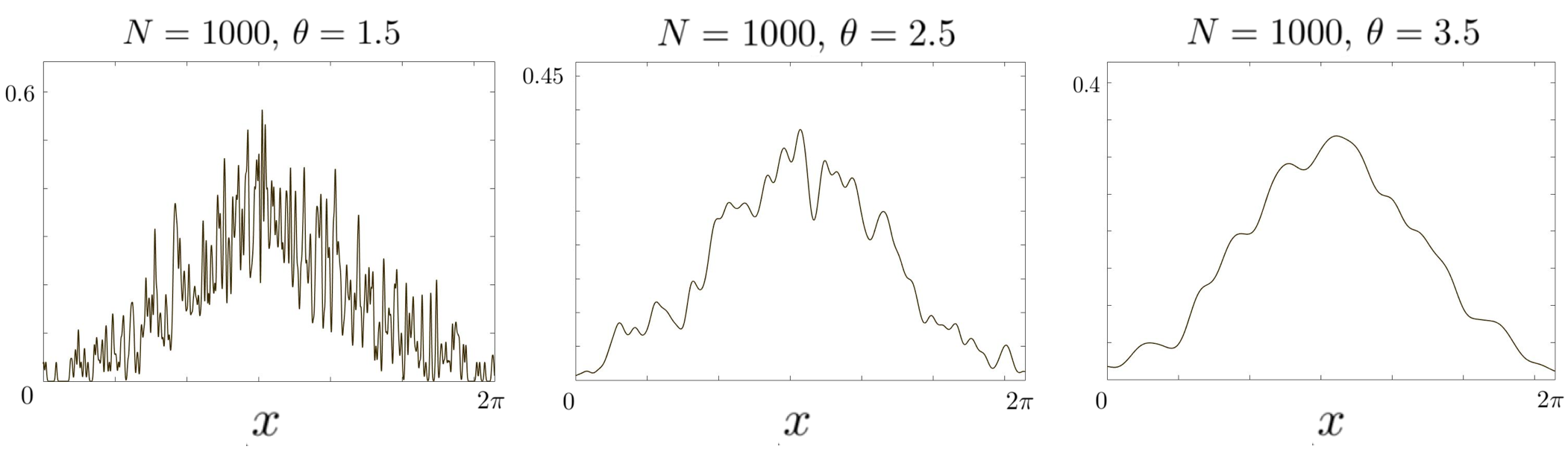
Figure 1: Numerical simulation of the $\epsilon$-smoothed local density $\rho_{\epsilon}(\cdot,t)=N^{-1}\sum_{i=1}^{N}{w_{\epsilon}(\cdot-q_{i}(t))}$ defined in (7), for a fixed time $t$, and on $D=[0,2\pi]$. In this specific example, $q_{i}(t)\sim\mathcal{N}(\pi,10^{0.2})$, $N=1000$, and $N$ and $\epsilon$ satisfy the scaling $N\epsilon^{\theta}=1$ for $\theta=1.5$ (left), $\theta=2.5$ (middle), $\theta=3.5$ (right). The smoothness of the density increases with $\theta$.

We use the $\epsilon$-smoothed quantities (7) instead of the original quantities (3) and follow the same guidelines described in Steps 1-2 of Subsection 1.1 in order to derive the regularised Dean–Kawasaki model. There, we will also consider the quantity

$$j_{2,\epsilon}(x,t):=\frac{1}{N}\sum_{i=1}^{N}{p^{2}_{i}(t)w^{\prime}_{\epsilon}(x-q_{i}(t))}.$$ (8)

We do not adapt Step 3 of Subsection 1.1, as we will not combine the equations for $\rho_{\epsilon},j_{\epsilon}$ or use the hydrodynamic limit theory.

We perform the analysis of the regularised Dean–Kawasaki model both for fixed values of $N$ and $\epsilon$, and also by means of a simultaneous limit involving $N\rightarrow\infty$ and $\epsilon\rightarrow 0$, for $N$ and $\epsilon$ satisfying a prescribed scaling. We first prove some preliminary uniform estimates for the three families of processes $\{\rho_{\epsilon}\}_{\epsilon}$ ,$\{j_{\epsilon}\}_{\epsilon}$, $\{j_{2,\epsilon}\}_{\epsilon}$ given in (7) and (8), as $\epsilon\rightarrow 0$. We have the following result.

Proposition 1.1 (Tightness of $\{\rho_{\epsilon}\}_{\epsilon},\{j_{\epsilon}\}_{\epsilon},\{j_{2,\epsilon}\}_{\epsilon}$).

Let $T>0$, and let $D\subset\mathbb{R}$ be a bounded domain. Assume the validity of either Assumption (G) or Assumption (NG), given below in Subsection 2.2. Then the families of processes of $\{\rho_{\epsilon}\}_{\epsilon},\{j_{\epsilon}\}_{\epsilon}$ are tight in $C(0,T;L^{2}(D))$ and $C(0,T;L^{4}(D))$, respectively, for $N\epsilon^{\theta}\geq 1$, with $\theta\geq 3$. In addition, the family $\{j_{2,\epsilon}\}_{\epsilon}$ is tight in $C(0,T;L^{4}(D))$ for $N\epsilon^{\theta}\geq 1$, with $\theta\geq 5$.

Proposition 1.1 yields relative compactness in law for the families of processes $\{\rho_{\epsilon}\}_{\epsilon},\{j_{\epsilon}\}_{\epsilon},\{j_{2,\epsilon}\}_{\epsilon}$ as $\epsilon\rightarrow 0$. We show convergence for the family $\{\rho_{\epsilon}\}_{\epsilon}$ as $\epsilon\rightarrow 0$ in the following result.

Proposition 1.2.

Let $T>0$, and let $D\subset\mathbb{R}$ be a bounded domain. Assume the validity of either Assumption (G) or Assumption (NG), as well as the scaling $N\epsilon^{\theta}\geq 1$, for some $\theta\geq 3$. For each $\epsilon>0$, let $\eta_{\epsilon}$ be the law of the process $\rho_{\epsilon}$ on $\mathcal{X}:=C(0,T;L^{2}(D))$. There exists a probability measure $\eta$ on $\mathcal{X}$ such that $\eta_{\epsilon}\stackrel{{\scriptstyle w}}{{\rightarrow}}\eta\mbox{ in }\mathcal{X}\mbox{ as }\epsilon\rightarrow 0$. Here $\stackrel{{\scriptstyle w}}{{\rightarrow}}$ denotes weak convergence of measures.

The proofs of Proposition 1.1 and 1.2 under Assumption (G) are the content of Subsection 3.1.

The next step, covered in Subsection 3.2, is the analysis of the evolution equations for $\rho_{\epsilon}$ and $j_{\epsilon}$, namely

$$\left\{\begin{array}[]{l}\vspace{-0.8 pc}\\ \displaystyle\frac{\partial\rho_{\epsilon}}{\partial t}(x,t)=-\frac{\partial j_{\epsilon}}{\partial x}(x,t),\vspace{-0.8 pc}\\ \displaystyle\frac{\partial j_{\epsilon}}{\partial t}(x,t)=\left(-\gamma j_{\epsilon}(x,t)-j_{2,\epsilon}(x,t)-\frac{1}{N}\sum_{i=1}^{N}{V^{\prime}(q_{i}(t))w_{\epsilon}(x-q_{i}(t))}\right)+\overbrace{\frac{\sigma}{N}\sum_{i=1}^{N}{w_{\epsilon}(x-q_{i}(t))\dot{\beta}_{i}}}^{=:\mathcal{\dot{Z}}_{N}(x,t)},\end{array}\right.$$ (9)

where $\mathcal{\dot{Z}}_{N}(x,t)$ is well-defined due to regularity of $w_{\epsilon}$ and of the processes $\{q_{i}\}_{i=1}^{N}$. System (9) is analogous to the system of evolution equations for the original quantities $\rho_{N},j_{N}$ mentioned in Step 1, see [24, Eq. (4)].

In analogy to the original derivation of the Dean–Kawasaki model, the noise $\mathcal{\dot{Z}}_{N}$ is not an elementary function of $\rho_{\epsilon}$ and $j_{\epsilon}$. For this reason, we rewrite $\mathcal{\dot{Z}}_{N}$ as

$$\mathcal{\dot{Z}}_{N}\sim\overbrace{\!\frac{\sigma}{\sqrt{N}}\sqrt{\rho_{\epsilon/\sqrt{2}}}\,\underbrace{Q^{1/2}_{\sqrt{2}\epsilon}\,\xi}_{=:\tilde{\xi}_{\epsilon}}}^{=:\mathcal{\dot{Y}}_{N}}+\mathcal{\dot{R}}_{N},$$ (10)

where $\sim$ denotes equality in law, $\xi$ is again a space-time white noise, $Q_{\sqrt{2}\epsilon}$ is the convolution operator with kernel $w_{\sqrt{2}\epsilon}$ on some spatial domain, and $\mathcal{\dot{R}}_{N}$ is a (small) stochastic remainder. The noise $\mathcal{\dot{Y}}_{N}$ is properly defined for non-negative function $\rho_{\epsilon}$. The specific structure of $\mathcal{\dot{Y}}_{N}$ is thoroughly discussed in Subsection 3.2. We estimate the “difference” between $\mathcal{\dot{Z}}_{N}$ and $\mathcal{\dot{Y}}_{N}$ (i.e., the remainder $\mathcal{\dot{R}}_{N}$) with the following result.

Theorem 1.3 (Error bounds for covariance structure in (9)).

Assume the validity of either Assumption (G) or Assumption (NG). Let $D\subset\mathbb{R}$ be a bounded set, and let $T>0$. Let $N,\epsilon$ satisfy the scaling $N\epsilon^{\theta}=1$, for some fixed $\theta\geq 7/2$. Let $Q_{\sqrt{2}\epsilon}\colon L^{2}(D)\rightarrow L^{2}(D)$ be the convolution operator with kernel $w_{\sqrt{2}\epsilon}$.

1. There exists $C=C(D,T)$ such that the following estimates concerning the spatial covariance of $\mathcal{Z}_{N}$ and $\mathcal{Y}_{N}$ hold for any $t\in[0,T]$ and $x_{1},x_{2}\in D$:

   $$\left|\mathbb{E}\left[\mathchoice{\raisebox{0.0pt}{$\displaystyle{\vphantom{\bigm{|}}\mathopen{}\mathcal{Z}_{N}(x_{1},t)\mathcal{Z}_{N}(x_{2},t)}$}}{\mathcal{Z}_{N}(x_{1},t)\mathcal{Z}_{N}(x_{2},t)}{\mathcal{Z}_{N}(x_{1},t)\mathcal{Z}_{N}(x_{2},t)}{\mathcal{Z}_{N}(x_{1},t)\mathcal{Z}_{N}(x_{2},t)}\right]-\mathbb{E}\left[\mathchoice{\raisebox{0.0pt}{$\displaystyle{\vphantom{\bigm{|}}\mathopen{}\mathcal{Y}_{N}(x_{1},t)\mathcal{Y}_{N}(x_{2},t)}$}}{\mathcal{Y}_{N}(x_{1},t)\mathcal{Y}_{N}(x_{2},t)}{\mathcal{Y}_{N}(x_{1},t)\mathcal{Y}_{N}(x_{2},t)}{\mathcal{Y}_{N}(x_{1},t)\mathcal{Y}_{N}(x_{2},t)}\right]\right| \leq\frac{C\sigma^{2}}{N}w_{\sqrt{2}\epsilon}(x_{1}-x_{2})|x_{1}-x_{2}|^{2},$$ (11)

   $$\left|\mathbb{E}\left[\mathchoice{\raisebox{0.0pt}{$\displaystyle{\vphantom{\bigm{|}}\mathopen{}\mathcal{Z}_{N}(x_{1},t)\mathcal{Z}_{N}(x_{2},t)}$}}{\mathcal{Z}_{N}(x_{1},t)\mathcal{Z}_{N}(x_{2},t)}{\mathcal{Z}_{N}(x_{1},t)\mathcal{Z}_{N}(x_{2},t)}{\mathcal{Z}_{N}(x_{1},t)\mathcal{Z}_{N}(x_{2},t)}\right]\right| \leq\frac{C\sigma^{2}}{N}w_{\sqrt{2}\epsilon}(x_{1}-x_{2}).$$ (12)

2. $\mathcal{Z}_{N}$ and $\mathcal{Y}_{N}$ decay to 0 as $N\rightarrow\infty$ and $\epsilon\rightarrow 0$. Specifically, for any $t\in[0,T]$ and any $x_{1}\in D$, we have

   $$\emph{Var}\left[\mathcal{Z}_{N}(x_{1},t)\right]\leq C\epsilon^{\theta-1},\qquad\emph{Var}\left[\mathcal{Y}_{N}(x_{1},t)\right]\leq C\epsilon^{\theta-1}.$$ (13)

Theorem 1.3, which is proved in Subsection 3.3 under Assumption (G), quantifies the error introduced when replacing the noise $\mathcal{\dot{Z}}_{N}$ with the multiplicative noise $\mathcal{\dot{Y}}_{N}$. More specifically, the bound in (11) is negligible for $x_{1}$, $x_{2}$ close to each other, when compared with the bound in (12). In addition, both $\mathcal{\dot{Z}}_{N}$ and $\mathcal{\dot{Y}}_{N}$ are negligible for distant $x_{1}$ and $x_{2}$. In combination with Proposition 1.1, Theorem 1.3 guarantees convergence of (9) to a deterministic system of equations, for $N\rightarrow\infty$ and $\epsilon\rightarrow 0$. This differs from the original Dean–Kawasaki model, as we have rescaled in the number of particles $N$.

Remark 1.4.

In the limit of infinitely many particles, $N\to\infty$, and under a local equilibrium assumption, one obtains as hydrodynamic limit (6) without the noise term and with the limit of $j_{2,\epsilon}$ being $j_{2}=\nabla\frac{\delta F(\rho)}{\delta\rho}$, for a suitable $F$. A justification of this can be found in the analysis of the Vlasov-Fokker-Planck equation, see for example [26, 9]. In contrast to our setting, the Vlasov-Fokker-Planck equation is derived by relying on the empirical density defined on the combined position–momentum state space, $\tilde{\rho}_{N}(x,y,t)=N^{-1}\sum_{i=1}^{N}{\delta(x-q_{i}(t),y-p_{i}(t))}$. In this work, we only use the position-dependent quantities (7)–(8), as this results in a more reduced model with half the spatial dimension (i.e., position as only space variable). In addition, we do not perform the aforementioned hydrodynamic limit, but then have to close the processes $j_{2,\epsilon}$ (for fixed $N$) using an approximation in the context of a low temperature regime for the underlying Langevin dynamics, see Subsection 3.5.

Subsection 3.4 is devoted to adapting the proofs of Proposition 1.1, Proposition 1.2, and Theorem 1.3 under Assumption (NG) instead of Assumption (G). Finally, in Subsection 3.5 we give suitable approximations of the components of (9) in order to obtain expressions closed in $\rho_{\epsilon}$, $j_{\epsilon}$, $V$.

Mild solutions to the regularised Dean–Kawasaki model in a periodic setting: In Section 4, we build on the contents of Subsection 3.5. We work on a periodic domain, in the case of a large number of particles $N$. We define the regularised Dean–Kawasaki model

$$\,\,\displaystyle\frac{\partial\rho_{\epsilon}}{\partial t}(x,t)=-\frac{\partial j_{\epsilon}}{\partial x}(x,t),\qquad x\in D=[0,2\pi],\,\,t\in[0,T],\vspace{0.7 pc}$$ (14a)

$$\,\,\displaystyle\frac{\partial j_{\epsilon}}{\partial t}(x,t)=-\gamma j_{\epsilon}(x,t)-\left(\frac{\sigma^{2}}{2\gamma}\right)\frac{\partial\rho_{\epsilon}}{\partial x}(x,t)-V_{\mathrm{per}}^{\prime}(x)\rho_{\epsilon}(x,t)+\frac{\sigma}{\sqrt{N}}\sqrt{\rho_{\epsilon}(x,t)}\,\tilde{\xi}_{\mathrm{per},\epsilon},\vspace{0.6 pc}$$ (14b)

$$\,\,\displaystyle\rho_{\epsilon}(x,0)=\rho_{0}(x),\quad j_{\epsilon}(x,0)=j_{0}(x).$$

Note that in addition to the approximations made in Subsection 3.5, we have also replaced $\tilde{\xi}_{\epsilon}$ and $V$ with $\tilde{\xi}_{\mathrm{per},\epsilon}$ and $V_{\mathrm{per}}$, the latter two being $2\pi$-periodic versions of the former. This is a natural choice for the analysis of the equations on a periodic domain.

Remark 1.5.

Equation (14) is a stochastic wave equation. Yet, standard well-posedness results for stochastic partial equations cannot be applied in a straightforward way. Firstly, unlike the stochastic heat equation with non-Lipschitz noise coefficient [30], equation (14) does not have a sufficiently regular Green function associated with its linear drift operator. This results in standard semigroup techniques not being able to provide well-posedness results for (14), due to the presence of the non-Lipschitz noise in (14b). Secondly, the theory of rough paths and paracontrolled distributions appears to be inapplicable, again due to the non-Lipschitz noise. Finally, the very nature of the wave equation does not seem to prevent $\rho$ from becoming negative (e.g., a suitable maximum principle appears to be unavailable), thus it unclear whether the noise is well-defined.

We prove various preliminary results associated with the existence theory for (14). These include the semigroup analysis associated with the deterministic integrand of (14) in Subsection 4.1, a discussion on the choice of a spatially periodic noise in Subsection 4.2, the analysis of the stochastic integrand of (14) in Subsection 4.3, preliminary existence and uniqueness results in Subsection 4.4, and a priori estimates in Subsections 4.5 and 4.6. Our key result, provided in Subsection 4.7, is the following.

Theorem 1.6 (High-probability existence and uniqueness result).

Let $D=[0,2\pi]$. Let $X_{0}=(\rho_{0},j_{0})\in H^{1}_{\mathrm{per}}(D)\times H^{1}_{\mathrm{per}}(D)$ be a deterministic initial condition, where $H^{1}_{\mathrm{per}}(D)$ denotes $2\pi$-periodic functions in $H^{1}(D)$. Assume that $\rho_{0}(x)\geq\eta$,$\mbox{ for all }x\in D$, for some $\eta>0$. Let the scaling $N\epsilon^{\theta}\geq 1$ be satisfied for some $\theta>7$, and let $\nu\in(0,1)$. It is possible to choose a sufficiently large number of particles $N$ such that there exists a unique $H^{1}_{\mathrm{per}}(D)\times H^{1}_{\mathrm{per}}(D)$-valued mild solution $X_{\epsilon}=(\rho_{\epsilon},j_{\epsilon})$ satisfying equation (14) up to a time $T=T(X_{0})$ on a set $F_{\nu}\in\mathcal{F}$ such that $\mathbb{P}(F_{\nu})\geq 1-\nu$. That is to say, the regularised Dean–Kawasaki model (14) is satisfied path-wise by a unique process $X_{\epsilon}$ on a set of probability at least $1-\nu$.

For the reader’s convenience, we summarise how we addressed the three difficulties of the original Dean–Kawasaki model. Firstly, we work in a function setting, thus the noise $\mathcal{\dot{Y}}_{N}$ is well-defined. Secondly, we do not combine the differential equations associated with $\rho_{\epsilon}$ (14a) and $j_{\epsilon}$ (14b), in contrast with [24]. On the contrary, we solve system (14) for the couple $(\rho_{\epsilon},j_{\epsilon})$, thus avoiding the formal application of the divergence operator for the stochastic noise of (9). Finally, we prove the above-mentioned high-probability existence and uniqueness result for (14).

The existence result of this paper is restricted to one spatial dimensional, $d=1$. This restriction comes from Sobolev embeddings, as we point out in Section 4.

Finally, Appendix A contains basic facts about Gaussian random variables, while Appendix B contains technical auxiliary results that are repeatedly used for the derivation of the regularised Dean–Kawasaki model carried out in Section 3.

Remark 1.7.

The assumptions of our main results (i.e., Proposition 1.1 and 1.2, and Theorems 1.3 and 1.6) are concerned with different scalings for the regularisation in $\epsilon$, namely $N\epsilon^{\theta}=1$ for some $\theta$, see Figure 1. The lower the value of $\theta$, the more general and less demanding the regularisation is. We motivate these scalings from the specific function spaces which are involved in the proofs of the aforementioned results. In this work, we do not fully analyse the optimality of such scalings (i.e., the indentification of the lowest admissible value of $\theta$). We limit ourselves to providing general comments on this matter in Remark 4.12.

2 Basic notation and assumptions

2.1 Basic Notation

We may use the same notation for different constants, even within the same line of computation. The dependence of a constant on given parameters will be highlighted only when it is relevant. We use the symbol $\|\cdot\|$ to denote the norm in $\mathbb{R}^{d}$. We use the symbol $\langle\cdot,\cdot\rangle$ to refer to the standard inner product in $\mathbb{R}^{d}$. For $x\in\mathbb{R}$, we define $\langle x\rangle:=\sqrt{1+x^{2}}$. The symbol $\mathbb{E}\left[X\right]$ denotes the expectation of a $\mathbb{R}^{d}$-valued random variable $X$ defined on the probability space $(\Omega,\mathcal{F},\mathbb{P})$. For two $\mathbb{R}^{d}$-valued random variables $X,Y$, we denote the covariance matrix (respectively, correlation matrix) of $X$ and $Y$ by $\mbox{Cov}(X,Y)$ (respectively, $\mbox{Corr}(X,Y)$). For a real-valued random variable $X$, we abbreviate $\mbox{Var}(X):=\mbox{Cov}(X,X)$. We will use the symbol $\sim$ to indicate equivalence of laws for random variables. In particular, we write $X\sim\mathcal{N}(\mu,\sigma^{2})$ for a Gaussian random variable $X$ of mean $\mu$ and variance $\sigma^{2}$. We write $\mathcal{G}(y,\mu,\sigma^{2})$ to denote the probability distribution function of $X\sim\mathcal{N}(\mu,\sigma^{2})$, namely $\mathcal{G}(y,\mu,\sigma^{2}):=(2\pi\sigma^{2})^{-1/2}\exp\left\{-(y-\mu)^{2}/(2\sigma^{2})\right\}$. Quite often, we will use the short-hand notation $w_{\epsilon}(y):=\mathcal{G}(y,0,\epsilon^{2})$, for $\epsilon>0$. For $X\sim\mathcal{N}(\mu,\sigma^{2})$, we define its absolute moments $M(n,\mu,\sigma^{2}):=\mathbb{E}\left[|X|^{n}\right]$ and plain moments $m(n,\mu,\sigma^{2}):=\mathbb{E}\left[X^{n}\right]$, for any $n\in\mathbb{N}\cup\{0\}$. For a vector $\mu\in\mathbb{R}^{d}$ and a symmetric semi-positive definite matrix $\Sigma\in\mathbb{R}^{d\times d}$, we write $X\sim\mathcal{N}(\mu,\Sigma)$ to denote an $\mathbb{R}^{d}$-valued Gaussian random vector with mean $\mu$ and covariance matrix $\Sigma$. For a domain $A\subset\mathbb{R}$, we use the standard notation $L^{p}(A)$ and $H^{n}(A)$ (for $p\in[1,\infty]$ and $n\in\mathbb{N}$) to denote the $L^{p}$-spaces on $A$ and the Sobolev spaces of functions on $A$ with square integrable weak derivatives up to order $n$. We denote $n$ times continuously differentiable functions on $A$ by $C^{n}(A)$ (for $n\in\mathbb{N}\cup\{\infty\}\cup\{0\}$).

2.2 Assumptions on the Langevin dynamics

We consider the following two different sets of assumptions associated with the Langevin dynamics (2), and in particular with the choice of potential $V$.

Assumption (G) (Gaussian setting for vanishing potential $V$).

Let $T>0$. The potential $V$ vanishes, $V\equiv 0$. Moreover, the initial condition $(q_{0},p_{0})$ to (2) is such that the solution $(q(t),p(t))$ to (2) satisfies

1. $(q(t),p(t))\mbox{ is a bivariate Gaussian vector}$, for all $t\in[0,T]$.

2. There exist $\iota>\nu>0$ such that $\nu\leq\mbox{\emph{Var}}[q(t)]\leq\iota$, for all $t\in[0,T]$.

3. The following quantities are Lipschitz on $[0,T]$: the expected values $\mu_{q}(t):=\mathbb{E}\left[\mathchoice{\raisebox{0.0pt}{$\displaystyle{\vphantom{\bigm{|}}\mathopen{}q(t)}$}}{q(t)}{q(t)}{q(t)}\right]$ and $\mu_{p}(t):=\mathbb{E}\left[\mathchoice{\raisebox{0.0pt}{$\displaystyle{\vphantom{\bigm{|}}\mathopen{}p(t)}$}}{p(t)}{p(t)}{p(t)}\right]$, the variances $\sigma^{2}_{q}(t):=\emph{Var}[q(t)]$ and $\sigma^{2}_{p}(t):=\emph{Var}[p(t)]$, and the correlation $\chi(t):=\emph{Corr}(q(t),p(t))$.

This assumption holds generically for the Ornstein-Uhlenbeck process dynamics, see Lemma A.6.

Assumption (NG) (Non-Gaussian setting for rapidly diverging $V(q)\approx|q|^{2n}$).

1. The potential $V$ is a $C^{\infty}(\mathbb{R})$-function. Furthermore, there exists $n\in\mathbb{N}$ such that, for all $k\in\mathbb{N}$, there exists a constant $C_{k}$ such that

   $$\left|\frac{\partial^{k}V(q)}{\partial q^{k}}\right|\leq C_{k}\left(1+\langle q\rangle^{2n-\min\{2,k\}}\right),\qquad\mbox{ for all }q\in\mathbb{R}.$$

2. There exist two constants $C_{0}(V),C_{1}(V)>0$ such that

   $$V(q)\geq C^{-1}_{0}\langle q\rangle^{2n}-C_{0},\qquad\left|\frac{\partial V(q)}{\partial q}\right|\geq C^{-1}_{1}\langle q\rangle^{2n-1}-C_{1},\qquad\mbox{ for all }q\in\mathbb{R}.$$

3. The joint density $g_{0}$ of the initial condition $(q_{0},p_{0})$ to (2) coincides with $\overline{g}(\overline{t},q,p)$, where $\overline{t}$ is some positive time and $\overline{g}(\overline{t},q,p)$ is the solution at time $\overline{t}$ to the Fokker–Planck equation

   $$\frac{\partial g}{\partial t}=-\nabla\cdot(g\mu)+\frac{\sigma^{2}}{2}\frac{\partial^{2}g}{\partial p^{2}},\qquad\mu:=\left(p,-\gamma p-V^{\prime}(q)\right),\qquad g(0,q,p)=\overline{g}_{0}(q,p),$$ (15)

   started from some initial condition $\overline{g}_{0}\in M^{1/2}H^{-5,-5}(\mathbb{R}^{2})$. The notation $H^{s,s}(\mathbb{R}^{2})$, $s>0$, denotes the $s^{th}$-order member of the isotropic Sobolev chain defined in [15, Eq. (3)], while the weight function $M(q,p)\propto\exp\left\{-(2\gamma/\sigma^{2})\left(p^{2}/2+V(q)\right)\right\}$ is the Gibbs invariant measure of (15).

4. We have that $\lim_{q\rightarrow+\infty}{V(q)/V(-q)}$ exists and is finite.

Items (i) and  (ii) of the Assumption (NG) are slightly more restrictive than those of [15, Hypotheses 1]. In particular, we assume the potential $V$ to diverge at infinity with no less than quadratic growth. This is encapsulated in the requirement $n\geq 1$ (instead of the requirement $n>1/2$ made in [15, Hypotheses 1]). Item (iii) implies regularity of the initial condition $g_{0}$.

We briefly justify the choice of the above two sets of hypotheses as follows. Assumption (G) guarantees the applicability of tools inherently associated with the theory of Gaussian random variables. Then many computations can be made explicit in a relatively straightforward way. On the other hand, Assumption (NG) is more general. Our analysis under Assumption (NG) is an extension of the argument previously carried out under Assumption (G). Both these assumptions will play a role in the derivation of the regularised Dean–Kawasaki model in Section 3.

3 Derivation of the regularised Dean–Kawasaki model

We now derive the regularised Dean–Kawasaki model studied in this paper. In Subsection 3.1, under Assumption (G), we prove a tightness result for the relevant quantities (7), (8), as well as uniqueness of the limit for the family $\{\rho_{\epsilon}\}_{\epsilon}$. These results are Propositions 1.1 and 1.2. The proof of Proposition 1.1 is nontrivial but also technical, and might be skipped at a first reading. Subsection 3.2 motivates the derivation of the noise $\mathcal{\dot{Y}}_{N}$, which we introduced in (10). In Subsection 3.3, under Assumption (G), we prove Theorem 1.3, which quantifies the difference between the noises $\mathcal{\dot{Y}}_{N}$ and $\mathcal{\dot{Z}}_{N}$ (see also (9)). In Subsection 3.4 we adapt the proofs of Propositions 1.1, 1.2, and Theorem 1.3 under Assumption (NG). Finally, Subsection 3.5 gathers the relevant information from the earlier parts of Section 3 in order to define a regularised Dean–Kawasaki model.

3.1 Tightness of leading quantities: proofs of Proposition 1.1 and Proposition 1.2

We prove some Kolmogorov-type tightness estimates for the families $\{\rho_{\epsilon}\}_{\epsilon}$, $\{j_{\epsilon}\}_{\epsilon}$ and $\{j_{2,\epsilon}\}_{\epsilon}$. The arguments are somewhat technical; as we are not aware of closely related results in the literature, we describe the proofs in some detail.

Proof of Proposition 1.1 under Assumption (G).

We verify the assumption of  [18, Corollary 14.9] for the families $\{\rho_{\epsilon}\}_{\epsilon}$, $\{j_{\epsilon}\}_{\epsilon}$, $\{j_{2,\epsilon}\}_{\epsilon}$. More specifically, for each family, we prove a suitable Kolmogorov time-regularity condition, as well as tightness of the processes at time 0.

Step 1: Tightness of $\{\rho_{\epsilon}\}_{\epsilon}$. We use the expansion of a square and the independence of the particles to write

$$\mathbb{E}\left[\mathchoice{\raisebox{0.0pt}{$\displaystyle{\vphantom{\bigm{|}}\mathopen{}\|\rho_{\epsilon}(\cdot,t)-\rho_{\epsilon}(\cdot,s)\|_{L^{2}(\mathbb{R})}^{2}}$}}{\|\rho_{\epsilon}(\cdot,t)-\rho_{\epsilon}(\cdot,s)\|_{L^{2}(\mathbb{R})}^{2}}{\|\rho_{\epsilon}(\cdot,t)-\rho_{\epsilon}(\cdot,s)\|_{L^{2}(\mathbb{R})}^{2}}{\|\rho_{\epsilon}(\cdot,t)-\rho_{\epsilon}(\cdot,s)\|_{L^{2}(\mathbb{R})}^{2}}\right]=\frac{1}{N^{2}}\mathbb{E}\left[\mathchoice{\raisebox{0.0pt}{$\displaystyle{\vphantom{\bigm{|}}\mathopen{}\!\int_{\mathbb{R}}{\!\sum_{i,j=1}^{N}{\!\left[w_{\epsilon}(x-q_{i}(t))-w_{\epsilon}(x-q_{i}(s))\right]\left[w_{\epsilon}(x-q_{j}(t))-w_{\epsilon}(x-q_{j}(s))\right]\mbox{d}x}}}$}}{\!\int_{\mathbb{R}}{\!\sum_{i,j=1}^{N}{\!\left[w_{\epsilon}(x-q_{i}(t))-w_{\epsilon}(x-q_{i}(s))\right]\left[w_{\epsilon}(x-q_{j}(t))-w_{\epsilon}(x-q_{j}(s))\right]\mbox{d}x}}}{\!\int_{\mathbb{R}}{\!\sum_{i,j=1}^{N}{\!\left[w_{\epsilon}(x-q_{i}(t))-w_{\epsilon}(x-q_{i}(s))\right]\left[w_{\epsilon}(x-q_{j}(t))-w_{\epsilon}(x-q_{j}(s))\right]\mbox{d}x}}}{\!\int_{\mathbb{R}}{\!\sum_{i,j=1}^{N}{\!\left[w_{\epsilon}(x-q_{i}(t))-w_{\epsilon}(x-q_{i}(s))\right]\left[w_{\epsilon}(x-q_{j}(t))-w_{\epsilon}(x-q_{j}(s))\right]\mbox{d}x}}}\right]$$

$$=\frac{1}{N^{2}}\sum_{i=1}^{N}{\mathbb{E}\left[\mathchoice{\raisebox{0.0pt}{$\displaystyle{\vphantom{\bigm{|}}\mathopen{}\left\|w_{\epsilon}(\cdot-q_{1}(t))-w_{\epsilon}(\cdot-q_{1}(s))\right\|^{2}_{L^{2}(\mathbb{R})}}$}}{\left\|w_{\epsilon}(\cdot-q_{1}(t))-w_{\epsilon}(\cdot-q_{1}(s))\right\|^{2}_{L^{2}(\mathbb{R})}}{\left\|w_{\epsilon}(\cdot-q_{1}(t))-w_{\epsilon}(\cdot-q_{1}(s))\right\|^{2}_{L^{2}(\mathbb{R})}}{\left\|w_{\epsilon}(\cdot-q_{1}(t))-w_{\epsilon}(\cdot-q_{1}(s))\right\|^{2}_{L^{2}(\mathbb{R})}}\right]}$$

$$\quad+\frac{1}{N^{2}}\sum_{i\neq j}{\int_{\mathbb{R}}{\mathbb{E}\left[\mathchoice{\raisebox{0.0pt}{$\displaystyle{\vphantom{\bigm{|}}\mathopen{}w_{\epsilon}(x-q_{i}(t))-w_{\epsilon}(x-q_{i}(s))}$}}{w_{\epsilon}(x-q_{i}(t))-w_{\epsilon}(x-q_{i}(s))}{w_{\epsilon}(x-q_{i}(t))-w_{\epsilon}(x-q_{i}(s))}{w_{\epsilon}(x-q_{i}(t))-w_{\epsilon}(x-q_{i}(s))}\right]\mathbb{E}\left[\mathchoice{\raisebox{0.0pt}{$\displaystyle{\vphantom{\bigm{|}}\mathopen{}w_{\epsilon}(x-q_{j}(t))-w_{\epsilon}(x-q_{j}(s))}$}}{w_{\epsilon}(x-q_{j}(t))-w_{\epsilon}(x-q_{j}(s))}{w_{\epsilon}(x-q_{j}(t))-w_{\epsilon}(x-q_{j}(s))}{w_{\epsilon}(x-q_{j}(t))-w_{\epsilon}(x-q_{j}(s))}\right]\mbox{d}x}}.$$

Given the identical distribution of the particles, we deduce

$$\mathbb{E}\left[\mathchoice{\raisebox{0.0pt}{$\displaystyle{\vphantom{\bigm{|}}\mathopen{}\|\rho_{\epsilon}(\cdot,t)-\rho_{\epsilon}(\cdot,s)\|_{L^{2}(\mathbb{R})}^{2}}$}}{\|\rho_{\epsilon}(\cdot,t)-\rho_{\epsilon}(\cdot,s)\|_{L^{2}(\mathbb{R})}^{2}}{\|\rho_{\epsilon}(\cdot,t)-\rho_{\epsilon}(\cdot,s)\|_{L^{2}(\mathbb{R})}^{2}}{\|\rho_{\epsilon}(\cdot,t)-\rho_{\epsilon}(\cdot,s)\|_{L^{2}(\mathbb{R})}^{2}}\right]$$

$$\quad=\frac{1}{N}\mathbb{E}\left[\mathchoice{\raisebox{0.0pt}{$\displaystyle{\vphantom{\bigm{|}}\mathopen{}\left\|w_{\epsilon}(\cdot-q_{1}(t))-w_{\epsilon}(\cdot-q_{1}(s))\right\|^{2}_{L^{2}(\mathbb{R})}}$}}{\left\|w_{\epsilon}(\cdot-q_{1}(t))-w_{\epsilon}(\cdot-q_{1}(s))\right\|^{2}_{L^{2}(\mathbb{R})}}{\left\|w_{\epsilon}(\cdot-q_{1}(t))-w_{\epsilon}(\cdot-q_{1}(s))\right\|^{2}_{L^{2}(\mathbb{R})}}{\left\|w_{\epsilon}(\cdot-q_{1}(t))-w_{\epsilon}(\cdot-q_{1}(s))\right\|^{2}_{L^{2}(\mathbb{R})}}\right]+\frac{1}{N^{2}}\sum_{i\neq j}\left\|\mathbb{E}\left[\mathchoice{\raisebox{0.0pt}{$\displaystyle{\vphantom{\bigm{|}}\mathopen{}w_{\epsilon}(\cdot-q_{1}(t))-w_{\epsilon}(\cdot-q_{1}(s))}$}}{w_{\epsilon}(\cdot-q_{1}(t))-w_{\epsilon}(\cdot-q_{1}(s))}{w_{\epsilon}(\cdot-q_{1}(t))-w_{\epsilon}(\cdot-q_{1}(s))}{w_{\epsilon}(\cdot-q_{1}(t))-w_{\epsilon}(\cdot-q_{1}(s))}\right]\right\|_{L^{2}(\mathbb{R})}^{2}$$

$$\quad\leq\frac{1}{N}\underbrace{\mathbb{E}\left[\mathchoice{\raisebox{0.0pt}{$\displaystyle{\vphantom{\bigm{|}}\mathopen{}\left\|w_{\epsilon}(\cdot-q_{1}(t))-w_{\epsilon}(\cdot-q_{1}(s))\right\|^{2}_{L^{2}(\mathbb{R})}}$}}{\left\|w_{\epsilon}(\cdot-q_{1}(t))-w_{\epsilon}(\cdot-q_{1}(s))\right\|^{2}_{L^{2}(\mathbb{R})}}{\left\|w_{\epsilon}(\cdot-q_{1}(t))-w_{\epsilon}(\cdot-q_{1}(s))\right\|^{2}_{L^{2}(\mathbb{R})}}{\left\|w_{\epsilon}(\cdot-q_{1}(t))-w_{\epsilon}(\cdot-q_{1}(s))\right\|^{2}_{L^{2}(\mathbb{R})}}\right]}_{=:I_{1}}+\underbrace{\left\|\mathbb{E}\left[\mathchoice{\raisebox{0.0pt}{$\displaystyle{\vphantom{\bigm{|}}\mathopen{}w_{\epsilon}(\cdot-q_{1}(t))-w_{\epsilon}(\cdot-q_{1}(s))}$}}{w_{\epsilon}(\cdot-q_{1}(t))-w_{\epsilon}(\cdot-q_{1}(s))}{w_{\epsilon}(\cdot-q_{1}(t))-w_{\epsilon}(\cdot-q_{1}(s))}{w_{\epsilon}(\cdot-q_{1}(t))-w_{\epsilon}(\cdot-q_{1}(s))}\right]\right\|_{L^{2}(\mathbb{R})}^{2}}_{=:\mathsf{ct}}.$$ (16)

There are two main differences between the term $I_{1}$ and the “cross-term” contribution $\mathsf{ct}$. Firstly, term $I_{1}$ is of the form $\mathbb{E}\left[\mathchoice{\raisebox{0.0pt}{$\displaystyle{\vphantom{\bigm{|}}\mathopen{}\|\cdot\|^{p}_{L^{p}(\mathbb{R})}}$}}{\|\cdot\|^{p}_{L^{p}(\mathbb{R})}}{\|\cdot\|^{p}_{L^{p}(\mathbb{R})}}{\|\cdot\|^{p}_{L^{p}(\mathbb{R})}}\right]$, while term $\mathsf{ct}$ is of the form $\|\mathbb{E}\left[\mathchoice{\raisebox{0.0pt}{$\displaystyle{\vphantom{\bigm{|}}\mathopen{}\cdot}$}}{\cdot}{\cdot}{\cdot}\right]\|^{p}_{L^{p}(\mathbb{R})}$. Secondly, term $\mathsf{ct}$ has no decaying scaling factor in $N$. This means that we are forced to provide a bound for $\mathsf{ct}$ which is independent of $\epsilon$. This bound is provided by invoking Lemmas B.2 and B.1. On the other hand, we are allowed to bound $I_{1}$ with quantities which might diverge in $\epsilon$ (these appear because of the form $\mathbb{E}\left[\mathchoice{\raisebox{0.0pt}{$\displaystyle{\vphantom{\bigm{|}}\mathopen{}\|\cdot\|^{p}_{L^{p}(\mathbb{R})}}$}}{\|\cdot\|^{p}_{L^{p}(\mathbb{R})}}{\|\cdot\|^{p}_{L^{p}(\mathbb{R})}}{\|\cdot\|^{p}_{L^{p}(\mathbb{R})}}\right]$, as we will point out), as long as they can be compensated by the scaling in $N$. These considerations are quite general, and we will apply similar reasonings at several points later on in the proof, as well as point out the relevant analogies when needed.

We occasionally drop the particle index, because of the identical distribution. We proceed to bound $I_{1}$ and $\mathsf{ct}$. Using the elementary inequality

$$1-e^{-x^{2}}\leq x^{2},\quad\mbox{ for all }x\in\mathbb{R},$$ (17)

we rewrite $I_{1}$ as

$$\mathbb{E}\left[\mathchoice{\raisebox{0.0pt}{$\displaystyle{\vphantom{\bigm{|}}\mathopen{}\left\|w_{\epsilon}(\cdot-q(t))-w_{\epsilon}(\cdot-q(s))\right\|_{L^{2}(\mathbb{R})}^{2}}$}}{\left\|w_{\epsilon}(\cdot-q(t))-w_{\epsilon}(\cdot-q(s))\right\|_{L^{2}(\mathbb{R})}^{2}}{\left\|w_{\epsilon}(\cdot-q(t))-w_{\epsilon}(\cdot-q(s))\right\|_{L^{2}(\mathbb{R})}^{2}}{\left\|w_{\epsilon}(\cdot-q(t))-w_{\epsilon}(\cdot-q(s))\right\|_{L^{2}(\mathbb{R})}^{2}}\right]=\mathbb{E}\left[\mathchoice{\raisebox{0.0pt}{$\displaystyle{\vphantom{\bigm{|}}\mathopen{}\int_{\mathbb{R}}{w^{2}_{\epsilon}(x-q(t))+w^{2}_{\epsilon}(x-q(s))-2w_{\epsilon}(x-q(t))w_{\epsilon}(x-q(s))}}$}}{\int_{\mathbb{R}}{w^{2}_{\epsilon}(x-q(t))+w^{2}_{\epsilon}(x-q(s))-2w_{\epsilon}(x-q(t))w_{\epsilon}(x-q(s))}}{\int_{\mathbb{R}}{w^{2}_{\epsilon}(x-q(t))+w^{2}_{\epsilon}(x-q(s))-2w_{\epsilon}(x-q(t))w_{\epsilon}(x-q(s))}}{\int_{\mathbb{R}}{w^{2}_{\epsilon}(x-q(t))+w^{2}_{\epsilon}(x-q(s))-2w_{\epsilon}(x-q(t))w_{\epsilon}(x-q(s))}}\right]$$

$$=\frac{1}{\sqrt{\pi\epsilon^{2}}}\,\mathbb{E}\left[\mathchoice{\raisebox{0.0pt}{$\displaystyle{\vphantom{\bigm{|}}\mathopen{}1-\exp\left(\frac{-(q(t)-q(s))^{2}}{4\epsilon^{2}}\right)}$}}{1-\exp\left(\frac{-(q(t)-q(s))^{2}}{4\epsilon^{2}}\right)}{1-\exp\left(\frac{-(q(t)-q(s))^{2}}{4\epsilon^{2}}\right)}{1-\exp\left(\frac{-(q(t)-q(s))^{2}}{4\epsilon^{2}}\right)}\right]\leq\frac{C}{\epsilon^{3}}\mathbb{E}\left[|q(t)-q(s)|^{2}\right]\leq\frac{C}{\epsilon^{3}}|t-s|^{2},$$ (18)

where we have used Lemma A.4 and an integration in $x$ in the last equality, and (17) in the first inequality. In addition, $q$ satisfies, by definition, the integral equation $q(t)-q(s)=\int_{s}^{t}{p(z)\mbox{d}z}$. The integrability properties of $p$ (Assumption (G)) and the Hölder inequality hence give the final inequality in (3.1). As for the cross-terms $\mathsf{ct}$, we employ Lemma B.2, estimate (87), and then apply Lemma B.1 to deduce

$$\left\|\mathchoice{\raisebox{0.0pt}{$\displaystyle{\vphantom{\bigm{|}}\mathopen{}\mathbb{E}\left[\mathchoice{\raisebox{0.0pt}{$\displaystyle{\vphantom{\bigm{|}}\mathopen{}w_{\epsilon}(\cdot-q(t))-w_{\epsilon}(\cdot-q(s))}$}}{w_{\epsilon}(\cdot-q(t))-w_{\epsilon}(\cdot-q(s))}{w_{\epsilon}(\cdot-q(t))-w_{\epsilon}(\cdot-q(s))}{w_{\epsilon}(\cdot-q(t))-w_{\epsilon}(\cdot-q(s))}\right]}$}}{\smash{\mathbb{E}\left[\mathchoice{\raisebox{0.0pt}{$\displaystyle{\vphantom{\bigm{|}}\mathopen{}w_{\epsilon}(\cdot-q(t))-w_{\epsilon}(\cdot-q(s))}$}}{w_{\epsilon}(\cdot-q(t))-w_{\epsilon}(\cdot-q(s))}{w_{\epsilon}(\cdot-q(t))-w_{\epsilon}(\cdot-q(s))}{w_{\epsilon}(\cdot-q(t))-w_{\epsilon}(\cdot-q(s))}\right]}}{\mathbb{E}\left[\mathchoice{\raisebox{0.0pt}{$\displaystyle{\vphantom{\bigm{|}}\mathopen{}w_{\epsilon}(\cdot-q(t))-w_{\epsilon}(\cdot-q(s))}$}}{w_{\epsilon}(\cdot-q(t))-w_{\epsilon}(\cdot-q(s))}{w_{\epsilon}(\cdot-q(t))-w_{\epsilon}(\cdot-q(s))}{w_{\epsilon}(\cdot-q(t))-w_{\epsilon}(\cdot-q(s))}\right]}{\mathbb{E}\left[\mathchoice{\raisebox{0.0pt}{$\displaystyle{\vphantom{\bigm{|}}\mathopen{}w_{\epsilon}(\cdot-q(t))-w_{\epsilon}(\cdot-q(s))}$}}{w_{\epsilon}(\cdot-q(t))-w_{\epsilon}(\cdot-q(s))}{w_{\epsilon}(\cdot-q(t))-w_{\epsilon}(\cdot-q(s))}{w_{\epsilon}(\cdot-q(t))-w_{\epsilon}(\cdot-q(s))}\right]}\right\|_{L^{2}(\mathbb{R})}^{2}=\int_{\mathbb{R}}{\left|\mathcal{G}(x,\mu(t),\sigma^{2}_{q}(t)+\epsilon^{2})-\mathcal{G}(x,\mu(s),\sigma^{2}_{q}(s)+\epsilon^{2})\right|^{2}\!\mbox{d}x}\leq C|t-s|^{2}.$$

We combine the estimates for $\mathsf{ct}$ and $I_{1}$ and obtain, thanks to the prescribed scaling $N\epsilon^{3}\geq 1$,

$$\mathbb{E}\left[\mathchoice{\raisebox{0.0pt}{$\displaystyle{\vphantom{\bigm{|}}\mathopen{}\|\rho_{\epsilon}(\cdot,t)-\rho_{\epsilon}(\cdot,s)\|_{L^{2}(\mathbb{R})}^{2}}$}}{\|\rho_{\epsilon}(\cdot,t)-\rho_{\epsilon}(\cdot,s)\|_{L^{2}(\mathbb{R})}^{2}}{\|\rho_{\epsilon}(\cdot,t)-\rho_{\epsilon}(\cdot,s)\|_{L^{2}(\mathbb{R})}^{2}}{\|\rho_{\epsilon}(\cdot,t)-\rho_{\epsilon}(\cdot,s)\|_{L^{2}(\mathbb{R})}^{2}}\right]\leq C\left(\frac{1}{N\epsilon^{3}}+1\right)|t-s|^{2}\leq C|t-s|^{2},$$

and the time regularity is settled using Kolmogorov’s continuity theorem. We now need to show that $\{\rho_{\epsilon}(\cdot,0)\}_{\epsilon}$ is tight in $L^{2}(D)$. We rely on the compact embedding $H^{1}(D)\subset L^{2}(D)$, see [2, Theorem 6.3], and we show that $\mathbb{E}\left[\mathchoice{\raisebox{0.0pt}{$\displaystyle{\vphantom{\bigm{|}}\mathopen{}\|\rho_{\epsilon}(\cdot,0)\|^{2}_{H^{1}(\mathbb{R})}}$}}{\|\rho_{\epsilon}(\cdot,0)\|^{2}_{H^{1}(\mathbb{R})}}{\|\rho_{\epsilon}(\cdot,0)\|^{2}_{H^{1}(\mathbb{R})}}{\|\rho_{\epsilon}(\cdot,0)\|^{2}_{H^{1}(\mathbb{R})}}\right]$ is uniformly bounded in $\epsilon$. A computation analogous to (3.1) gives

$$\mathbb{E}\left[\mathchoice{\raisebox{0.0pt}{$\displaystyle{\vphantom{\bigm{|}}\mathopen{}\|\rho_{\epsilon}(\cdot,0)\|^{2}_{H^{1}(\mathbb{R})}}$}}{\|\rho_{\epsilon}(\cdot,0)\|^{2}_{H^{1}(\mathbb{R})}}{\|\rho_{\epsilon}(\cdot,0)\|^{2}_{H^{1}(\mathbb{R})}}{\|\rho_{\epsilon}(\cdot,0)\|^{2}_{H^{1}(\mathbb{R})}}\right]=\mathbb{E}\left[\mathchoice{\raisebox{0.0pt}{$\displaystyle{\vphantom{\bigm{|}}\mathopen{}\|\rho_{\epsilon}(\cdot,0)\|^{2}_{L^{2}(\mathbb{R})}}$}}{\|\rho_{\epsilon}(\cdot,0)\|^{2}_{L^{2}(\mathbb{R})}}{\|\rho_{\epsilon}(\cdot,0)\|^{2}_{L^{2}(\mathbb{R})}}{\|\rho_{\epsilon}(\cdot,0)\|^{2}_{L^{2}(\mathbb{R})}}\right]+\mathbb{E}\left[\mathchoice{\raisebox{0.0pt}{$\displaystyle{\vphantom{\bigm{|}}\mathopen{}\left\|\frac{\partial\rho_{\epsilon}}{\partial x}(\cdot,0)\right\|^{2}_{L^{2}(\mathbb{R})}}$}}{\left\|\frac{\partial\rho_{\epsilon}}{\partial x}(\cdot,0)\right\|^{2}_{L^{2}(\mathbb{R})}}{\left\|\frac{\partial\rho_{\epsilon}}{\partial x}(\cdot,0)\right\|^{2}_{L^{2}(\mathbb{R})}}{\left\|\frac{\partial\rho_{\epsilon}}{\partial x}(\cdot,0)\right\|^{2}_{L^{2}(\mathbb{R})}}\right]$$

$$\quad\leq\frac{1}{N}\underbrace{\mathbb{E}\left[\mathchoice{\raisebox{0.0pt}{$\displaystyle{\vphantom{\bigm{|}}\mathopen{}\int_{\mathbb{R}}{w^{2}_{\epsilon}(x-q_{1}(0))\mbox{d}x+w^{\prime 2}_{\epsilon}(x-q_{1}(0))\mbox{d}x}}$}}{\int_{\mathbb{R}}{w^{2}_{\epsilon}(x-q_{1}(0))\mbox{d}x+w^{\prime 2}_{\epsilon}(x-q_{1}(0))\mbox{d}x}}{\int_{\mathbb{R}}{w^{2}_{\epsilon}(x-q_{1}(0))\mbox{d}x+w^{\prime 2}_{\epsilon}(x-q_{1}(0))\mbox{d}x}}{\int_{\mathbb{R}}{w^{2}_{\epsilon}(x-q_{1}(0))\mbox{d}x+w^{\prime 2}_{\epsilon}(x-q_{1}(0))\mbox{d}x}}\right]}_{=:I_{1}}+\underbrace{\int_{\mathbb{R}}{\mathbb{E}\left[\mathchoice{\raisebox{0.0pt}{$\displaystyle{\vphantom{\bigm{|}}\mathopen{}w_{\epsilon}(x-q_{1}(0))}$}}{w_{\epsilon}(x-q_{1}(0))}{w_{\epsilon}(x-q_{1}(0))}{w_{\epsilon}(x-q_{1}(0))}\right]^{2}+\mathbb{E}\left[\mathchoice{\raisebox{0.0pt}{$\displaystyle{\vphantom{\bigm{|}}\mathopen{}w^{\prime}_{\epsilon}(x-q_{1}(0))}$}}{w^{\prime}_{\epsilon}(x-q_{1}(0))}{w^{\prime}_{\epsilon}(x-q_{1}(0))}{w^{\prime}_{\epsilon}(x-q_{1}(0))}\right]^{2}\mbox{d}x.}}_{=:\mathsf{ct}}$$ (19)

The bound $I_{1}\leq C\epsilon^{-3}$ follows from Lemma A.4, in combination with the integration in $x$ and the definition of the Gaussian moments, see Lemma A.5. The term $\mathsf{ct}$ can be bounded uniformly in $\epsilon$ using Lemma B.2, estimates (87) and (88). The scaling $N\epsilon^{3}\geq 1$ finally implies tightness for $\{\rho_{\epsilon}\}_{\epsilon}$.

Step 2: Tightness of $\{j_{\epsilon}\}_{\epsilon}$. For notational convenience, we define

$$\tau_{i}(x,s,t):=p_{i}(t)w_{\epsilon}(x-q_{i}(t))-p_{i}(s)w_{\epsilon}(x-q_{i}(s)),$$

so that $j_{\epsilon}(x,t)-j_{\epsilon}(x,s)=N^{-1}\sum_{i=1}^{N}{\tau_{i}(x,s,t)}$. In the same fashion as (3.1), we expand

$$\mathbb{E}\left[\mathchoice{\raisebox{0.0pt}{$\displaystyle{\vphantom{\bigm{|}}\mathopen{}\left\|\mathchoice{\raisebox{0.0pt}{$\displaystyle{\vphantom{\bigm{|}}\mathopen{}j_{\epsilon}(\cdot,t)-j_{\epsilon}(\cdot,s)}$}}{\smash{j_{\epsilon}(\cdot,t)-j_{\epsilon}(\cdot,s)}}{j_{\epsilon}(\cdot,t)-j_{\epsilon}(\cdot,s)}{j_{\epsilon}(\cdot,t)-j_{\epsilon}(\cdot,s)}\right\|_{L^{4}(\mathbb{R})}^{4}}$}}{\left\|\mathchoice{\raisebox{0.0pt}{$\displaystyle{\vphantom{\bigm{|}}\mathopen{}j_{\epsilon}(\cdot,t)-j_{\epsilon}(\cdot,s)}$}}{\smash{j_{\epsilon}(\cdot,t)-j_{\epsilon}(\cdot,s)}}{j_{\epsilon}(\cdot,t)-j_{\epsilon}(\cdot,s)}{j_{\epsilon}(\cdot,t)-j_{\epsilon}(\cdot,s)}\right\|_{L^{4}(\mathbb{R})}^{4}}{\left\|\mathchoice{\raisebox{0.0pt}{$\displaystyle{\vphantom{\bigm{|}}\mathopen{}j_{\epsilon}(\cdot,t)-j_{\epsilon}(\cdot,s)}$}}{\smash{j_{\epsilon}(\cdot,t)-j_{\epsilon}(\cdot,s)}}{j_{\epsilon}(\cdot,t)-j_{\epsilon}(\cdot,s)}{j_{\epsilon}(\cdot,t)-j_{\epsilon}(\cdot,s)}\right\|_{L^{4}(\mathbb{R})}^{4}}{\left\|\mathchoice{\raisebox{0.0pt}{$\displaystyle{\vphantom{\bigm{|}}\mathopen{}j_{\epsilon}(\cdot,t)-j_{\epsilon}(\cdot,s)}$}}{\smash{j_{\epsilon}(\cdot,t)-j_{\epsilon}(\cdot,s)}}{j_{\epsilon}(\cdot,t)-j_{\epsilon}(\cdot,s)}{j_{\epsilon}(\cdot,t)-j_{\epsilon}(\cdot,s)}\right\|_{L^{4}(\mathbb{R})}^{4}}\right]\leq\frac{1}{N^{3}}\underbrace{\int_{\mathbb{R}}{\mathbb{E}\left[\mathchoice{\raisebox{0.0pt}{$\displaystyle{\vphantom{\bigm{|}}\mathopen{}\tau_{1}(x,s,t)^{4}}$}}{\tau_{1}(x,s,t)^{4}}{\tau_{1}(x,s,t)^{4}}{\tau_{1}(x,s,t)^{4}}\right]\mbox{d}x}}_{=:I_{1}}+\frac{C}{N^{2}}\underbrace{\int_{\mathbb{R}}{\mathbb{E}\left[\mathchoice{\raisebox{0.0pt}{$\displaystyle{\vphantom{\bigm{|}}\mathopen{}\left|\tau_{1}(x,s,t)\right|}$}}{\left|\tau_{1}(x,s,t)\right|}{\left|\tau_{1}(x,s,t)\right|}{\left|\tau_{1}(x,s,t)\right|}\right]\mathbb{E}\left[\mathchoice{\raisebox{0.0pt}{$\displaystyle{\vphantom{\bigm{|}}\mathopen{}\left|\tau^{3}_{1}(x,s,t)\right|}$}}{\left|\tau^{3}_{1}(x,s,t)\right|}{\left|\tau^{3}_{1}(x,s,t)\right|}{\left|\tau^{3}_{1}(x,s,t)\right|}\right]\mbox{d}x}}_{=:I_{2}}$$

$$\quad+\frac{C}{N^{2}}\underbrace{\int_{\mathbb{R}}{\mathbb{E}\left[\mathchoice{\raisebox{0.0pt}{$\displaystyle{\vphantom{\bigm{|}}\mathopen{}\tau^{2}_{1}(x,s,t)}$}}{\tau^{2}_{1}(x,s,t)}{\tau^{2}_{1}(x,s,t)}{\tau^{2}_{1}(x,s,t)}\right]^{2}}\mbox{d}x}_{=:I_{3}}+\frac{C}{N}\underbrace{\int_{\mathbb{R}}{\mathbb{E}\left[\mathchoice{\raisebox{0.0pt}{$\displaystyle{\vphantom{\bigm{|}}\mathopen{}\tau_{1}(x,s,t)}$}}{\tau_{1}(x,s,t)}{\tau_{1}(x,s,t)}{\tau_{1}(x,s,t)}\right]^{2}\mathbb{E}\left[\mathchoice{\raisebox{0.0pt}{$\displaystyle{\vphantom{\bigm{|}}\mathopen{}\tau^{2}_{1}(x,s,t)}$}}{\tau^{2}_{1}(x,s,t)}{\tau^{2}_{1}(x,s,t)}{\tau^{2}_{1}(x,s,t)}\right]}\mbox{d}x}_{=:I_{4}}+\underbrace{\int_{\mathbb{R}}{\mathbb{E}\left[\mathchoice{\raisebox{0.0pt}{$\displaystyle{\vphantom{\bigm{|}}\mathopen{}\tau_{1}(x,s,t)}$}}{\tau_{1}(x,s,t)}{\tau_{1}(x,s,t)}{\tau_{1}(x,s,t)}\right]^{4}}\mbox{d}x}_{=:\mathsf{ct}}.$$ (20)

The discussion following (3.1) applies analogously to the family of terms $I_{1}$, $I_{2}$, $I_{3}$ and $I_{4}$, which do contain at least one term of the form $\mathbb{E}\left[\mathchoice{\raisebox{0.0pt}{$\displaystyle{\vphantom{\bigm{|}}\mathopen{}\tau_{i}(x,s,t)^{p}}$}}{\tau_{i}(x,s,t)^{p}}{\tau_{i}(x,s,t)^{p}}{\tau_{i}(x,s,t)^{p}}\right]$, and to the term $\mathsf{ct}$, which is of the form $\|\mathbb{E}\left[\mathchoice{\raisebox{0.0pt}{$\displaystyle{\vphantom{\bigm{|}}\mathopen{}\cdot}$}}{\cdot}{\cdot}{\cdot}\right]\|^{p}_{L^{p}(\mathbb{R})}$. We thus provide an $\epsilon$-independent bound for $\mathsf{ct}$, and suitable $\epsilon$-diverging bounds for $I_{1}$, $I_{2}$, $I_{3}$ and $I_{4}$.

The conditional density for bivariate Gaussian random variables, stated in Lemma A.3, implies

$$f_{p(t)|q(t)}(p|q(t)=b)=\mathcal{G}\left(p,\mu_{p}(t)+\frac{\sigma_{p}(t)}{\sigma_{q}(t)}\chi(t)(b-\mu_{q}(t)),(1-\chi(t)^{2})\sigma^{2}_{p}(t)\right),\qquad\mbox{for all }b\in\mathbb{R}.$$ (21)

We use the law of total expectation and (21) to compute

$$\mathbb{E}\left[\mathchoice{\raisebox{0.0pt}{$\displaystyle{\vphantom{\bigm{|}}\mathopen{}p(t)w_{\epsilon}(x-q(t))}$}}{p(t)w_{\epsilon}(x-q(t))}{p(t)w_{\epsilon}(x-q(t))}{p(t)w_{\epsilon}(x-q(t))}\right] =\mathbb{E}\left[\mathchoice{\raisebox{0.0pt}{$\displaystyle{\vphantom{\bigm{|}}\mathopen{}\mathbb{E}\left[\mathchoice{\raisebox{0.0pt}{$\displaystyle{\vphantom{\bigm{|}}\mathopen{}p(t)w_{\epsilon}(x-q(t))|q(t)}$}}{p(t)w_{\epsilon}(x-q(t))|q(t)}{p(t)w_{\epsilon}(x-q(t))|q(t)}{p(t)w_{\epsilon}(x-q(t))|q(t)}\right]}$}}{\mathbb{E}\left[\mathchoice{\raisebox{0.0pt}{$\displaystyle{\vphantom{\bigm{|}}\mathopen{}p(t)w_{\epsilon}(x-q(t))|q(t)}$}}{p(t)w_{\epsilon}(x-q(t))|q(t)}{p(t)w_{\epsilon}(x-q(t))|q(t)}{p(t)w_{\epsilon}(x-q(t))|q(t)}\right]}{\mathbb{E}\left[\mathchoice{\raisebox{0.0pt}{$\displaystyle{\vphantom{\bigm{|}}\mathopen{}p(t)w_{\epsilon}(x-q(t))|q(t)}$}}{p(t)w_{\epsilon}(x-q(t))|q(t)}{p(t)w_{\epsilon}(x-q(t))|q(t)}{p(t)w_{\epsilon}(x-q(t))|q(t)}\right]}{\mathbb{E}\left[\mathchoice{\raisebox{0.0pt}{$\displaystyle{\vphantom{\bigm{|}}\mathopen{}p(t)w_{\epsilon}(x-q(t))|q(t)}$}}{p(t)w_{\epsilon}(x-q(t))|q(t)}{p(t)w_{\epsilon}(x-q(t))|q(t)}{p(t)w_{\epsilon}(x-q(t))|q(t)}\right]}\right]=\mathbb{E}\left[\mathchoice{\raisebox{0.0pt}{$\displaystyle{\vphantom{\bigm{|}}\mathopen{}w_{\epsilon}(x-q(t))\left(\mu_{p}(t)+\frac{\sigma_{p}(t)}{\sigma_{q}(t)}\chi(t)(q(t)-\mu_{q}(t))\right)}$}}{w_{\epsilon}(x-q(t))\left(\mu_{p}(t)+\frac{\sigma_{p}(t)}{\sigma_{q}(t)}\chi(t)(q(t)-\mu_{q}(t))\right)}{w_{\epsilon}(x-q(t))\left(\mu_{p}(t)+\frac{\sigma_{p}(t)}{\sigma_{q}(t)}\chi(t)(q(t)-\mu_{q}(t))\right)}{w_{\epsilon}(x-q(t))\left(\mu_{p}(t)+\frac{\sigma_{p}(t)}{\sigma_{q}(t)}\chi(t)(q(t)-\mu_{q}(t))\right)}\right]$$

$$=a_{1}(t)\mathbb{E}\left[\mathchoice{\raisebox{0.0pt}{$\displaystyle{\vphantom{\bigm{|}}\mathopen{}w_{\epsilon}(x-q(t))}$}}{w_{\epsilon}(x-q(t))}{w_{\epsilon}(x-q(t))}{w_{\epsilon}(x-q(t))}\right]+a_{2}(t)\mathbb{E}\left[\mathchoice{\raisebox{0.0pt}{$\displaystyle{\vphantom{\bigm{|}}\mathopen{}w_{\epsilon}(x-q(t))q(t)}$}}{w_{\epsilon}(x-q(t))q(t)}{w_{\epsilon}(x-q(t))q(t)}{w_{\epsilon}(x-q(t))q(t)}\right],$$ (22)

where we set

$$a_{1}(t):=\mu_{p}(t)-\frac{\sigma_{p}(t)}{\sigma_{q}(t)}\chi(t)\mu_{q}(t),\quad a_{2}(t):=\frac{\sigma_{p}(t)}{\sigma_{q}(t)}\chi(t).$$

The time-dependent coefficients $a_{1}$ and $a_{2}$ are Lipschitz, thanks to Assumption (G). Keeping in mind Remark B.3, we use Lemma B.2, estimate (87) and then Lemma B.1. We deduce

$$\mathsf{ct}\leq C|t-s|^{1+\beta},$$ (23)

for some $\beta\in(0,1)$.

We now treat the $\epsilon$-diverging terms $I_{1}$, $I_{2}$, $I_{3}$ and $I_{4}$ in (3.1). By adding and subtracting the quantity $2p(t)p(s)w_{\epsilon/\sqrt{2}}(x-(q(t)+q(s))/2)$, using (17), and integrating in $x$, we obtain

$$\int_{\mathbb{R}}{\mathbb{E}\left[\mathchoice{\raisebox{0.0pt}{$\displaystyle{\vphantom{\bigm{|}}\mathopen{}\tau^{2}_{1}(x,s,t)}$}}{\tau^{2}_{1}(x,s,t)}{\tau^{2}_{1}(x,s,t)}{\tau^{2}_{1}(x,s,t)}\right]\mbox{d}x} =\frac{1}{\sqrt{4\pi\epsilon^{2}}}\mathbb{E}\left[\mathchoice{\raisebox{0.0pt}{$\displaystyle{\vphantom{\bigm{|}}\mathopen{}\int_{\mathbb{R}}{p^{2}(t)w_{\frac{\epsilon}{\sqrt{2}}}(x-q(t))+p^{2}(s)w_{\frac{\epsilon}{\sqrt{2}}}(x-q(s))}\mbox{d}x}$}}{\int_{\mathbb{R}}{p^{2}(t)w_{\frac{\epsilon}{\sqrt{2}}}(x-q(t))+p^{2}(s)w_{\frac{\epsilon}{\sqrt{2}}}(x-q(s))}\mbox{d}x}{\int_{\mathbb{R}}{p^{2}(t)w_{\frac{\epsilon}{\sqrt{2}}}(x-q(t))+p^{2}(s)w_{\frac{\epsilon}{\sqrt{2}}}(x-q(s))}\mbox{d}x}{\int_{\mathbb{R}}{p^{2}(t)w_{\frac{\epsilon}{\sqrt{2}}}(x-q(t))+p^{2}(s)w_{\frac{\epsilon}{\sqrt{2}}}(x-q(s))}\mbox{d}x}\right]+$$

$$\quad-\frac{1}{\sqrt{4\pi\epsilon^{2}}}\mathbb{E}\left[\mathchoice{\raisebox{0.0pt}{$\displaystyle{\vphantom{\bigm{|}}\mathopen{}\int_{\mathbb{R}}{2p(t)p(s)\exp\left\{-\frac{(q(t)-q(s))^{2}}{4\epsilon^{2}}\right\}w_{\frac{\epsilon}{\sqrt{2}}}\left(x-\frac{q(t)+q(s)}{2}\right)}\mbox{d}x}$}}{\int_{\mathbb{R}}{2p(t)p(s)\exp\left\{-\frac{(q(t)-q(s))^{2}}{4\epsilon^{2}}\right\}w_{\frac{\epsilon}{\sqrt{2}}}\left(x-\frac{q(t)+q(s)}{2}\right)}\mbox{d}x}{\int_{\mathbb{R}}{2p(t)p(s)\exp\left\{-\frac{(q(t)-q(s))^{2}}{4\epsilon^{2}}\right\}w_{\frac{\epsilon}{\sqrt{2}}}\left(x-\frac{q(t)+q(s)}{2}\right)}\mbox{d}x}{\int_{\mathbb{R}}{2p(t)p(s)\exp\left\{-\frac{(q(t)-q(s))^{2}}{4\epsilon^{2}}\right\}w_{\frac{\epsilon}{\sqrt{2}}}\left(x-\frac{q(t)+q(s)}{2}\right)}\mbox{d}x}\right]$$

$$=\frac{1}{\sqrt{4\pi\epsilon^{2}}}\mathbb{E}\left[\mathchoice{\raisebox{0.0pt}{$\displaystyle{\vphantom{\bigm{|}}\mathopen{}|p(t)-p(s)|^{2}}$}}{|p(t)-p(s)|^{2}}{|p(t)-p(s)|^{2}}{|p(t)-p(s)|^{2}}\right]+\frac{1}{\sqrt{4\pi\epsilon^{2}}}\mathbb{E}\left[\mathchoice{\raisebox{0.0pt}{$\displaystyle{\vphantom{\bigm{|}}\mathopen{}2p(s)p(t)\left(1-\exp\left\{-\frac{(q(t)-q(s))^{2}}{4\epsilon^{2}}\right\}\right)}$}}{2p(s)p(t)\left(1-\exp\left\{-\frac{(q(t)-q(s))^{2}}{4\epsilon^{2}}\right\}\right)}{2p(s)p(t)\left(1-\exp\left\{-\frac{(q(t)-q(s))^{2}}{4\epsilon^{2}}\right\}\right)}{2p(s)p(t)\left(1-\exp\left\{-\frac{(q(t)-q(s))^{2}}{4\epsilon^{2}}\right\}\right)}\right]$$

$$\leq\frac{1}{\sqrt{4\pi\epsilon^{2}}}\mathbb{E}\left[\mathchoice{\raisebox{0.0pt}{$\displaystyle{\vphantom{\bigm{|}}\mathopen{}|p(t)-p(s)|^{2}}$}}{|p(t)-p(s)|^{2}}{|p(t)-p(s)|^{2}}{|p(t)-p(s)|^{2}}\right]+\frac{C}{\epsilon^{3}}\mathbb{E}\left[\mathchoice{\raisebox{0.0pt}{$\displaystyle{\vphantom{\bigm{|}}\mathopen{}2p(s)p(t)\left|q(t)-q(s)\right|^{2}}$}}{2p(s)p(t)\left|q(t)-q(s)\right|^{2}}{2p(s)p(t)\left|q(t)-q(s)\right|^{2}}{2p(s)p(t)\left|q(t)-q(s)\right|^{2}}\right].$$ (24)

The first expectation in the last line of (3.1) satisfies $\mathbb{E}\left[\mathchoice{\raisebox{0.0pt}{$\displaystyle{\vphantom{\bigm{|}}\mathopen{}|p(t)-p(s)|^{2}}$}}{|p(t)-p(s)|^{2}}{|p(t)-p(s)|^{2}}{|p(t)-p(s)|^{2}}\right]\leq C|t-s|$. This is implied by the Itô isometry, which we invoke because $p$ satisfies, by definition, the stochastic integral equation $p(t)-p(s)=\int_{s}^{t}{-\gamma p(z)\mbox{d}z}+\sigma\int_{s}^{t}{\mbox{d}\beta(z)}$. Note the difference in time regularity with the previously discussed $\mathbb{E}\left[\mathchoice{\raisebox{0.0pt}{$\displaystyle{\vphantom{\bigm{|}}\mathopen{}|q(t)-q(s)|^{2}}$}}{|q(t)-q(s)|^{2}}{|q(t)-q(s)|^{2}}{|q(t)-q(s)|^{2}}\right]$, see (3.1). As for the second expectation in the last line of (3.1), we may use the Hölder inequality on the probability space to separate $p(s)p(t)$ from $\left|q(t)-q(s)\right|^{2}$. Using again the integrability of $p$ granted by Assumption (G) and the Hölder inequality in time for $q(t)-q(s)$, we deduce

$$\int_{\mathbb{R}}{\mathbb{E}\left[\mathchoice{\raisebox{0.0pt}{$\displaystyle{\vphantom{\bigm{|}}\mathopen{}\tau^{2}_{1}(x,s,t)}$}}{\tau^{2}_{1}(x,s,t)}{\tau^{2}_{1}(x,s,t)}{\tau^{2}_{1}(x,s,t)}\right]\mbox{d}x}\leq\frac{C}{\epsilon}|t-s|+\frac{C}{\epsilon^{3}}|t-s|^{2}.$$ (25)

In addition, we have the bound ${\mathbb{E}\left[\mathchoice{\raisebox{0.0pt}{$\displaystyle{\vphantom{\bigm{|}}\mathopen{}\tau_{1}(x,s,t)}$}}{\tau_{1}(x,s,t)}{\tau_{1}(x,s,t)}{\tau_{1}(x,s,t)}\right]^{2}}\leq C|t-s|$, where $C$ is independent of $x$ and $\epsilon$. This can be justified by relying on (3.1), using the fact that right-hand-side of (87) (for $X$ being the process $q$) is Lipschitz in time, with Lipschitz constant independent of $\epsilon$ and $x$, as explained in Remark B.3. Hence, using (25), we deduce that

$$I_{4}\leq\frac{C}{N\epsilon^{3}}|t-s|^{2}.$$

We have completed the analysis for $I_{4}$, which is the term that requires the most care, due to the fact that it is paired with the slowest decay in $N$ as coefficient. As for the other terms $I_{1}$, $I_{2}$ and $I_{3}$, we need not provide sharp bounds. By repeatedly applying the Hölder inequality on the probability space $\Omega$, we deduce that $I_{2}$ and $I_{3}$ are bounded by $I_{1}$. We therefore only need to provide an estimate for $I_{1}$ in order to conclude Step (ii). We write

$$I_{1}\leq C\,\mathbb{E}\left[\mathchoice{\raisebox{0.0pt}{$\displaystyle{\vphantom{\bigm{|}}\mathopen{}\int_{\mathbb{R}}{(p(t)-p(s))^{4}w^{4}_{\epsilon}(x-q(t))}\mbox{d}x}$}}{\int_{\mathbb{R}}{(p(t)-p(s))^{4}w^{4}_{\epsilon}(x-q(t))}\mbox{d}x}{\int_{\mathbb{R}}{(p(t)-p(s))^{4}w^{4}_{\epsilon}(x-q(t))}\mbox{d}x}{\int_{\mathbb{R}}{(p(t)-p(s))^{4}w^{4}_{\epsilon}(x-q(t))}\mbox{d}x}\right]+C\,\mathbb{E}\left[\mathchoice{\raisebox{0.0pt}{$\displaystyle{\vphantom{\bigm{|}}\mathopen{}\int_{\mathbb{R}}{p(s)^{4}(w_{\epsilon}(x-q(t))-w_{\epsilon}(x-q(s)))^{4}}\mbox{d}x}$}}{\int_{\mathbb{R}}{p(s)^{4}(w_{\epsilon}(x-q(t))-w_{\epsilon}(x-q(s)))^{4}}\mbox{d}x}{\int_{\mathbb{R}}{p(s)^{4}(w_{\epsilon}(x-q(t))-w_{\epsilon}(x-q(s)))^{4}}\mbox{d}x}{\int_{\mathbb{R}}{p(s)^{4}(w_{\epsilon}(x-q(t))-w_{\epsilon}(x-q(s)))^{4}}\mbox{d}x}\right].$$ (26)

We reuse some algebraic computations from (3.1) to continue as

$$I_{1} \leq C\,\mathbb{E}\left[\mathchoice{\raisebox{0.0pt}{$\displaystyle{\vphantom{\bigm{|}}\mathopen{}\int_{\mathbb{R}}{(p(t)-p(s))^{4}w^{4}_{\epsilon}(x-q(t))}\mbox{d}x}$}}{\int_{\mathbb{R}}{(p(t)-p(s))^{4}w^{4}_{\epsilon}(x-q(t))}\mbox{d}x}{\int_{\mathbb{R}}{(p(t)-p(s))^{4}w^{4}_{\epsilon}(x-q(t))}\mbox{d}x}{\int_{\mathbb{R}}{(p(t)-p(s))^{4}w^{4}_{\epsilon}(x-q(t))}\mbox{d}x}\right]+C\,\mathbb{E}\left[\mathchoice{\raisebox{0.0pt}{$\displaystyle{\vphantom{\bigm{|}}\mathopen{}\int_{\mathbb{R}}{p(s)^{4}(w_{\epsilon}(x-q(t))-w_{\epsilon}(x-q(s)))^{4}}\mbox{d}x}$}}{\int_{\mathbb{R}}{p(s)^{4}(w_{\epsilon}(x-q(t))-w_{\epsilon}(x-q(s)))^{4}}\mbox{d}x}{\int_{\mathbb{R}}{p(s)^{4}(w_{\epsilon}(x-q(t))-w_{\epsilon}(x-q(s)))^{4}}\mbox{d}x}{\int_{\mathbb{R}}{p(s)^{4}(w_{\epsilon}(x-q(t))-w_{\epsilon}(x-q(s)))^{4}}\mbox{d}x}\right]$$

$$\leq\frac{C}{\epsilon^{4}}\mathbb{E}\left[\mathchoice{\raisebox{0.0pt}{$\displaystyle{\vphantom{\bigm{|}}\mathopen{}(p(t)-p(s))^{4}}$}}{(p(t)-p(s))^{4}}{(p(t)-p(s))^{4}}{(p(t)-p(s))^{4}}\right]+C\mathbb{E}\left[\mathchoice{\raisebox{0.0pt}{$\displaystyle{\vphantom{\bigm{|}}\mathopen{}p^{4}(s)\frac{C}{\epsilon^{2}}\int_{\mathbb{R}}{(w_{\epsilon}(x-q(t))-w_{\epsilon}(x-q(s)))^{2}}\mbox{d}x}$}}{p^{4}(s)\frac{C}{\epsilon^{2}}\int_{\mathbb{R}}{(w_{\epsilon}(x-q(t))-w_{\epsilon}(x-q(s)))^{2}}\mbox{d}x}{p^{4}(s)\frac{C}{\epsilon^{2}}\int_{\mathbb{R}}{(w_{\epsilon}(x-q(t))-w_{\epsilon}(x-q(s)))^{2}}\mbox{d}x}{p^{4}(s)\frac{C}{\epsilon^{2}}\int_{\mathbb{R}}{(w_{\epsilon}(x-q(t))-w_{\epsilon}(x-q(s)))^{2}}\mbox{d}x}\right]$$

$$\leq\frac{C}{\epsilon^{4}}\mathbb{E}\left[\mathchoice{\raisebox{0.0pt}{$\displaystyle{\vphantom{\bigm{|}}\mathopen{}(p(t)-p(s))^{4}}$}}{(p(t)-p(s))^{4}}{(p(t)-p(s))^{4}}{(p(t)-p(s))^{4}}\right]+\frac{C}{\epsilon^{2}}\mathbb{E}\left[\mathchoice{\raisebox{0.0pt}{$\displaystyle{\vphantom{\bigm{|}}\mathopen{}p^{4}(s)\frac{1}{\epsilon}\left(1-\exp\left(-\frac{(q(t)-q(s))^{2}}{4\epsilon^{2}}\right)\right)}$}}{p^{4}(s)\frac{1}{\epsilon}\left(1-\exp\left(-\frac{(q(t)-q(s))^{2}}{4\epsilon^{2}}\right)\right)}{p^{4}(s)\frac{1}{\epsilon}\left(1-\exp\left(-\frac{(q(t)-q(s))^{2}}{4\epsilon^{2}}\right)\right)}{p^{4}(s)\frac{1}{\epsilon}\left(1-\exp\left(-\frac{(q(t)-q(s))^{2}}{4\epsilon^{2}}\right)\right)}\right]$$

$$\leq\frac{C}{\epsilon^{4}}\mathbb{E}\left[\mathchoice{\raisebox{0.0pt}{$\displaystyle{\vphantom{\bigm{|}}\mathopen{}(p(t)-p(s))^{4}}$}}{(p(t)-p(s))^{4}}{(p(t)-p(s))^{4}}{(p(t)-p(s))^{4}}\right]+\frac{C}{\epsilon^{5}}\mathbb{E}\left[\mathchoice{\raisebox{0.0pt}{$\displaystyle{\vphantom{\bigm{|}}\mathopen{}p^{4}(s)(q(t)-q(s))^{2}}$}}{p^{4}(s)(q(t)-q(s))^{2}}{p^{4}(s)(q(t)-q(s))^{2}}{p^{4}(s)(q(t)-q(s))^{2}}\right]$$

$$\leq\frac{C}{\epsilon^{4}}|t-s|^{2}+\frac{C}{\epsilon^{5}}\mathbb{E}\left[\mathchoice{\raisebox{0.0pt}{$\displaystyle{\vphantom{\bigm{|}}\mathopen{}p^{8}(s)}$}}{p^{8}(s)}{p^{8}(s)}{p^{8}(s)}\right]^{1/2}\mathbb{E}\left[\mathchoice{\raisebox{0.0pt}{$\displaystyle{\vphantom{\bigm{|}}\mathopen{}(q(t)-q(s))^{4}}$}}{(q(t)-q(s))^{4}}{(q(t)-q(s))^{4}}{(q(t)-q(s))^{4}}\right]^{1/2}\leq\frac{C}{\epsilon^{5}}|t-s|^{2}.$$

In particular, we have used the bound $\max_{y}{w_{\epsilon}(y)}\leq C\epsilon^{-1}$ in the second inequality, Lemma A.4 in the third inequality, (17) in the fourth inequality, and integrability properties of $p$ and $q$ in the fifth and sixth inequality. The scaling $N\epsilon^{3}\geq 1$ concludes the time regularity analysis for $\{j_{\epsilon}\}_{\epsilon}$. As for the tightness of $\{j_{\epsilon}(\cdot,0)\}_{\epsilon}$, we deal with the analogous expression of (3.1) for $\{j_{\epsilon}\}_{\epsilon}$. The analysis is similar, apart from the use of Lemma A.3 prior to the use of Lemma B.2 (for the corresponding term $\mathsf{ct}$) and the use of the compact embedding $H^{1}(D)\subset L^{4}(D)$.

Step 3: Tightness of $\{j_{2,\epsilon}\}_{\epsilon}$. For notational convenience, we define

$$\tau_{i}(x,s,t):=p^{2}_{i}(t)w^{\prime}_{\epsilon}(x-q_{i}(t))-p^{2}_{i}(s)w^{\prime}_{\epsilon}(x-q_{i}(s)),$$

so that $j_{2,\epsilon}(x,t)-j_{2,\epsilon}(x,s)=N^{-1}\sum_{i=1}^{N}{\tau_{i}(x,s,t)}$. In the same fashion as (3.1), we expand

$$\mathbb{E}\left[\mathchoice{\raisebox{0.0pt}{$\displaystyle{\vphantom{\bigm{|}}\mathopen{}\left\|\mathchoice{\raisebox{0.0pt}{$\displaystyle{\vphantom{\bigm{|}}\mathopen{}j_{2,\epsilon}(\cdot,t)-j_{2,\epsilon}(\cdot,s)}$}}{\smash{j_{2,\epsilon}(\cdot,t)-j_{2,\epsilon}(\cdot,s)}}{j_{2,\epsilon}(\cdot,t)-j_{2,\epsilon}(\cdot,s)}{j_{2,\epsilon}(\cdot,t)-j_{2,\epsilon}(\cdot,s)}\right\|_{L^{4}(\mathbb{R})}^{4}}$}}{\left\|\mathchoice{\raisebox{0.0pt}{$\displaystyle{\vphantom{\bigm{|}}\mathopen{}j_{2,\epsilon}(\cdot,t)-j_{2,\epsilon}(\cdot,s)}$}}{\smash{j_{2,\epsilon}(\cdot,t)-j_{2,\epsilon}(\cdot,s)}}{j_{2,\epsilon}(\cdot,t)-j_{2,\epsilon}(\cdot,s)}{j_{2,\epsilon}(\cdot,t)-j_{2,\epsilon}(\cdot,s)}\right\|_{L^{4}(\mathbb{R})}^{4}}{\left\|\mathchoice{\raisebox{0.0pt}{$\displaystyle{\vphantom{\bigm{|}}\mathopen{}j_{2,\epsilon}(\cdot,t)-j_{2,\epsilon}(\cdot,s)}$}}{\smash{j_{2,\epsilon}(\cdot,t)-j_{2,\epsilon}(\cdot,s)}}{j_{2,\epsilon}(\cdot,t)-j_{2,\epsilon}(\cdot,s)}{j_{2,\epsilon}(\cdot,t)-j_{2,\epsilon}(\cdot,s)}\right\|_{L^{4}(\mathbb{R})}^{4}}{\left\|\mathchoice{\raisebox{0.0pt}{$\displaystyle{\vphantom{\bigm{|}}\mathopen{}j_{2,\epsilon}(\cdot,t)-j_{2,\epsilon}(\cdot,s)}$}}{\smash{j_{2,\epsilon}(\cdot,t)-j_{2,\epsilon}(\cdot,s)}}{j_{2,\epsilon}(\cdot,t)-j_{2,\epsilon}(\cdot,s)}{j_{2,\epsilon}(\cdot,t)-j_{2,\epsilon}(\cdot,s)}\right\|_{L^{4}(\mathbb{R})}^{4}}\right]\leq\frac{1}{N^{3}}\underbrace{\int_{\mathbb{R}}{\mathbb{E}\left[\mathchoice{\raisebox{0.0pt}{$\displaystyle{\vphantom{\bigm{|}}\mathopen{}\tau_{1}(x,s,t)^{4}}$}}{\tau_{1}(x,s,t)^{4}}{\tau_{1}(x,s,t)^{4}}{\tau_{1}(x,s,t)^{4}}\right]}\mbox{d}x}_{=:I_{1}}+\frac{C}{N^{2}}\underbrace{\int_{\mathbb{R}}{\mathbb{E}\left[\mathchoice{\raisebox{0.0pt}{$\displaystyle{\vphantom{\bigm{|}}\mathopen{}\left|\tau_{1}(x,s,t)\right|}$}}{\left|\tau_{1}(x,s,t)\right|}{\left|\tau_{1}(x,s,t)\right|}{\left|\tau_{1}(x,s,t)\right|}\right]\mathbb{E}\left[\mathchoice{\raisebox{0.0pt}{$\displaystyle{\vphantom{\bigm{|}}\mathopen{}\left|\tau^{3}_{1}(x,s,t)\right|}$}}{\left|\tau^{3}_{1}(x,s,t)\right|}{\left|\tau^{3}_{1}(x,s,t)\right|}{\left|\tau^{3}_{1}(x,s,t)\right|}\right]}\mbox{d}x}_{=:I_{2}}$$

$$\quad+\frac{C}{N^{2}}\underbrace{\int_{\mathbb{R}}{\mathbb{E}\left[\mathchoice{\raisebox{0.0pt}{$\displaystyle{\vphantom{\bigm{|}}\mathopen{}\tau^{2}_{1}(x,s,t)}$}}{\tau^{2}_{1}(x,s,t)}{\tau^{2}_{1}(x,s,t)}{\tau^{2}_{1}(x,s,t)}\right]^{2}}\mbox{d}x}_{=:I_{3}}+\frac{C}{N}\underbrace{\int_{\mathbb{R}}{\mathbb{E}\left[\mathchoice{\raisebox{0.0pt}{$\displaystyle{\vphantom{\bigm{|}}\mathopen{}\tau_{1}(x,s,t)}$}}{\tau_{1}(x,s,t)}{\tau_{1}(x,s,t)}{\tau_{1}(x,s,t)}\right]^{2}\mathbb{E}\left[\mathchoice{\raisebox{0.0pt}{$\displaystyle{\vphantom{\bigm{|}}\mathopen{}\tau^{2}_{1}(x,s,t)}$}}{\tau^{2}_{1}(x,s,t)}{\tau^{2}_{1}(x,s,t)}{\tau^{2}_{1}(x,s,t)}\right]}\mbox{d}x}_{=:I_{4}}+\underbrace{\int_{\mathbb{R}}{\mathbb{E}\left[\mathchoice{\raisebox{0.0pt}{$\displaystyle{\vphantom{\bigm{|}}\mathopen{}\tau_{1}(x,s,t)}$}}{\tau_{1}(x,s,t)}{\tau_{1}(x,s,t)}{\tau_{1}(x,s,t)}\right]^{4}}\mbox{d}x}_{=:\mathsf{ct}}.$$ (27)

The considerations for $I_{1}$, $I_{2}$, $I_{3}$ and $I_{4}$ and $\mathsf{ct}$ are analogous to the ones for the homonymous counterparts in (3.1). In order to estimate $\mathsf{ct}$, we need to compute $\mathbb{E}\left[\mathchoice{\raisebox{0.0pt}{$\displaystyle{\vphantom{\bigm{|}}\mathopen{}p^{2}(t)w^{\prime}_{\epsilon}(x-q(t))}$}}{p^{2}(t)w^{\prime}_{\epsilon}(x-q(t))}{p^{2}(t)w^{\prime}_{\epsilon}(x-q(t))}{p^{2}(t)w^{\prime}_{\epsilon}(x-q(t))}\right]$. We again rely on the conditional law (21) and the law of total expectation to write

$$\mathbb{E}\left[\mathchoice{\raisebox{0.0pt}{$\displaystyle{\vphantom{\bigm{|}}\mathopen{}p^{2}(t)w^{\prime}_{\epsilon}(x-q(t))}$}}{p^{2}(t)w^{\prime}_{\epsilon}(x-q(t))}{p^{2}(t)w^{\prime}_{\epsilon}(x-q(t))}{p^{2}(t)w^{\prime}_{\epsilon}(x-q(t))}\right] =\mathbb{E}\left[\mathchoice{\raisebox{0.0pt}{$\displaystyle{\vphantom{\bigm{|}}\mathopen{}\mathbb{E}\left[\mathchoice{\raisebox{0.0pt}{$\displaystyle{\vphantom{\bigm{|}}\mathopen{}p^{2}(t)w^{\prime}_{\epsilon}(x-q(t))|q(t)}$}}{p^{2}(t)w^{\prime}_{\epsilon}(x-q(t))|q(t)}{p^{2}(t)w^{\prime}_{\epsilon}(x-q(t))|q(t)}{p^{2}(t)w^{\prime}_{\epsilon}(x-q(t))|q(t)}\right]}$}}{\mathbb{E}\left[\mathchoice{\raisebox{0.0pt}{$\displaystyle{\vphantom{\bigm{|}}\mathopen{}p^{2}(t)w^{\prime}_{\epsilon}(x-q(t))|q(t)}$}}{p^{2}(t)w^{\prime}_{\epsilon}(x-q(t))|q(t)}{p^{2}(t)w^{\prime}_{\epsilon}(x-q(t))|q(t)}{p^{2}(t)w^{\prime}_{\epsilon}(x-q(t))|q(t)}\right]}{\mathbb{E}\left[\mathchoice{\raisebox{0.0pt}{$\displaystyle{\vphantom{\bigm{|}}\mathopen{}p^{2}(t)w^{\prime}_{\epsilon}(x-q(t))|q(t)}$}}{p^{2}(t)w^{\prime}_{\epsilon}(x-q(t))|q(t)}{p^{2}(t)w^{\prime}_{\epsilon}(x-q(t))|q(t)}{p^{2}(t)w^{\prime}_{\epsilon}(x-q(t))|q(t)}\right]}{\mathbb{E}\left[\mathchoice{\raisebox{0.0pt}{$\displaystyle{\vphantom{\bigm{|}}\mathopen{}p^{2}(t)w^{\prime}_{\epsilon}(x-q(t))|q(t)}$}}{p^{2}(t)w^{\prime}_{\epsilon}(x-q(t))|q(t)}{p^{2}(t)w^{\prime}_{\epsilon}(x-q(t))|q(t)}{p^{2}(t)w^{\prime}_{\epsilon}(x-q(t))|q(t)}\right]}\right]$$

$$=\mathbb{E}\left[\mathchoice{\raisebox{0.0pt}{$\displaystyle{\vphantom{\bigm{|}}\mathopen{}w^{\prime}_{\epsilon}(x-q(t))\left\{(\mu_{p}(t)+\frac{\sigma_{p}(t)}{\sigma_{q}(t)}\chi(t)(q(t)-\mu_{q}(t)))^{2}+(1-\chi^{2}(t))\sigma^{2}_{p}(t)\right\}}$}}{w^{\prime}_{\epsilon}(x-q(t))\left\{(\mu_{p}(t)+\frac{\sigma_{p}(t)}{\sigma_{q}(t)}\chi(t)(q(t)-\mu_{q}(t)))^{2}+(1-\chi^{2}(t))\sigma^{2}_{p}(t)\right\}}{w^{\prime}_{\epsilon}(x-q(t))\left\{(\mu_{p}(t)+\frac{\sigma_{p}(t)}{\sigma_{q}(t)}\chi(t)(q(t)-\mu_{q}(t)))^{2}+(1-\chi^{2}(t))\sigma^{2}_{p}(t)\right\}}{w^{\prime}_{\epsilon}(x-q(t))\left\{(\mu_{p}(t)+\frac{\sigma_{p}(t)}{\sigma_{q}(t)}\chi(t)(q(t)-\mu_{q}(t)))^{2}+(1-\chi^{2}(t))\sigma^{2}_{p}(t)\right\}}\right].$$ (28)

The right-hand-side of (3.1), thanks to Assumption (G), Lemma B.2 and Remark B.3, is of the form prescribed by Lemma B.1. Hence we deduce

$$\mathsf{ct}\leq C|t-s|^{1+\beta},\qquad\mbox{for some }\beta>0.$$

The analysis of terms $I_{1}$, $I_{2}$, $I_{3}$, $I_{4}$ in (3.1) is similar to the one we carried out for the homonymous terms in (3.1). We set $\tilde{q}:=(q(t)+q(s))/2$ and use Lemma A.4 to compute

$$\int_{\mathbb{R}}{\mathbb{E}\left[\mathchoice{\raisebox{0.0pt}{$\displaystyle{\vphantom{\bigm{|}}\mathopen{}\tau^{2}_{1}(x,s,t)}$}}{\tau^{2}_{1}(x,s,t)}{\tau^{2}_{1}(x,s,t)}{\tau^{2}_{1}(x,s,t)}\right]\mbox{d}x} =\frac{1}{\sqrt{4\pi\epsilon^{2}}}\frac{1}{\epsilon^{4}}\left\{\mathbb{E}\left[\mathchoice{\raisebox{0.0pt}{$\displaystyle{\vphantom{\bigm{|}}\mathopen{}\int_{\mathbb{R}}{p^{4}(t)w_{\frac{\epsilon}{\sqrt{2}}}(x-q(t))(q(t)-x)^{2}+p^{4}(s)w_{\frac{\epsilon}{\sqrt{2}}}(x-q(s))(q(s)-x)^{2}}\mbox{d}x}$}}{\int_{\mathbb{R}}{p^{4}(t)w_{\frac{\epsilon}{\sqrt{2}}}(x-q(t))(q(t)-x)^{2}+p^{4}(s)w_{\frac{\epsilon}{\sqrt{2}}}(x-q(s))(q(s)-x)^{2}}\mbox{d}x}{\int_{\mathbb{R}}{p^{4}(t)w_{\frac{\epsilon}{\sqrt{2}}}(x-q(t))(q(t)-x)^{2}+p^{4}(s)w_{\frac{\epsilon}{\sqrt{2}}}(x-q(s))(q(s)-x)^{2}}\mbox{d}x}{\int_{\mathbb{R}}{p^{4}(t)w_{\frac{\epsilon}{\sqrt{2}}}(x-q(t))(q(t)-x)^{2}+p^{4}(s)w_{\frac{\epsilon}{\sqrt{2}}}(x-q(s))(q(s)-x)^{2}}\mbox{d}x}\right]\right.+$$

$$\quad-\left.2\mathbb{E}\left[\mathchoice{\raisebox{0.0pt}{$\displaystyle{\vphantom{\bigm{|}}\mathopen{}\int_{\mathbb{R}}{p^{2}(t)p^{2}(s)\exp\left\{-\frac{(q(t)-q(s))^{2}}{4\epsilon^{2}}\right\}w_{\frac{\epsilon}{\sqrt{2}}}\left(x-\tilde{q}\right)\underbrace{(q(t)-x)(q(s)-x)}_{=:T_{1}}}\mbox{d}x}$}}{\int_{\mathbb{R}}{p^{2}(t)p^{2}(s)\exp\left\{-\frac{(q(t)-q(s))^{2}}{4\epsilon^{2}}\right\}w_{\frac{\epsilon}{\sqrt{2}}}\left(x-\tilde{q}\right)\underbrace{(q(t)-x)(q(s)-x)}_{=:T_{1}}}\mbox{d}x}{\int_{\mathbb{R}}{p^{2}(t)p^{2}(s)\exp\left\{-\frac{(q(t)-q(s))^{2}}{4\epsilon^{2}}\right\}w_{\frac{\epsilon}{\sqrt{2}}}\left(x-\tilde{q}\right)\underbrace{(q(t)-x)(q(s)-x)}_{=:T_{1}}}\mbox{d}x}{\int_{\mathbb{R}}{p^{2}(t)p^{2}(s)\exp\left\{-\frac{(q(t)-q(s))^{2}}{4\epsilon^{2}}\right\}w_{\frac{\epsilon}{\sqrt{2}}}\left(x-\tilde{q}\right)\underbrace{(q(t)-x)(q(s)-x)}_{=:T_{1}}}\mbox{d}x}\right]\right\}.$$

We add and subtract $\tilde{q}$ in both brackets of $T_{1}$. Similarly to the argument in (3.1), we rely on the $x$-integration with Gaussian kernels, the trivial bound $e^{z}\leq 1$ for $z\leq 0$, and we continue the above estimate

$$\int_{\mathbb{R}}{\mathbb{E}\left[\mathchoice{\raisebox{0.0pt}{$\displaystyle{\vphantom{\bigm{|}}\mathopen{}\tau^{2}_{1}(x,s,t)}$}}{\tau^{2}_{1}(x,s,t)}{\tau^{2}_{1}(x,s,t)}{\tau^{2}_{1}(x,s,t)}\right]\mbox{d}x} \leq\frac{C}{\epsilon^{3}}\mathbb{E}\left[\mathchoice{\raisebox{0.0pt}{$\displaystyle{\vphantom{\bigm{|}}\mathopen{}p^{4}(t)+p^{4}(s)-2p^{2}(t)p^{2}(s)+2p^{2}(t)p^{2}(s)\left(1-\exp\left\{-\frac{(q(t)-q(s))^{2}}{4\epsilon^{2}}\right\}\right)}$}}{p^{4}(t)+p^{4}(s)-2p^{2}(t)p^{2}(s)+2p^{2}(t)p^{2}(s)\left(1-\exp\left\{-\frac{(q(t)-q(s))^{2}}{4\epsilon^{2}}\right\}\right)}{p^{4}(t)+p^{4}(s)-2p^{2}(t)p^{2}(s)+2p^{2}(t)p^{2}(s)\left(1-\exp\left\{-\frac{(q(t)-q(s))^{2}}{4\epsilon^{2}}\right\}\right)}{p^{4}(t)+p^{4}(s)-2p^{2}(t)p^{2}(s)+2p^{2}(t)p^{2}(s)\left(1-\exp\left\{-\frac{(q(t)-q(s))^{2}}{4\epsilon^{2}}\right\}\right)}\right]$$

$$\quad+\frac{C}{\epsilon^{5}}\mathbb{E}\left[\mathchoice{\raisebox{0.0pt}{$\displaystyle{\vphantom{\bigm{|}}\mathopen{}\int_{\mathbb{R}}{p^{2}(t)p^{2}(s)\exp\left\{-\frac{(q(t)-q(s))^{2}}{4\epsilon^{2}}\right\}\left|q(t)-q(s)\right|^{2}}\mbox{d}x}$}}{\int_{\mathbb{R}}{p^{2}(t)p^{2}(s)\exp\left\{-\frac{(q(t)-q(s))^{2}}{4\epsilon^{2}}\right\}\left|q(t)-q(s)\right|^{2}}\mbox{d}x}{\int_{\mathbb{R}}{p^{2}(t)p^{2}(s)\exp\left\{-\frac{(q(t)-q(s))^{2}}{4\epsilon^{2}}\right\}\left|q(t)-q(s)\right|^{2}}\mbox{d}x}{\int_{\mathbb{R}}{p^{2}(t)p^{2}(s)\exp\left\{-\frac{(q(t)-q(s))^{2}}{4\epsilon^{2}}\right\}\left|q(t)-q(s)\right|^{2}}\mbox{d}x}\right]$$

$$\leq\frac{C}{\epsilon^{3}}\mathbb{E}\left[\mathchoice{\raisebox{0.0pt}{$\displaystyle{\vphantom{\bigm{|}}\mathopen{}\left|p^{2}(t)-p^{2}(s)\right|^{2}}$}}{\left|p^{2}(t)-p^{2}(s)\right|^{2}}{\left|p^{2}(t)-p^{2}(s)\right|^{2}}{\left|p^{2}(t)-p^{2}(s)\right|^{2}}\right]+\frac{C}{\epsilon^{5}}\mathbb{E}\left[\mathchoice{\raisebox{0.0pt}{$\displaystyle{\vphantom{\bigm{|}}\mathopen{}p^{2}(t)p^{2}(s)|q(t)-q(s)|^{2}}$}}{p^{2}(t)p^{2}(s)|q(t)-q(s)|^{2}}{p^{2}(t)p^{2}(s)|q(t)-q(s)|^{2}}{p^{2}(t)p^{2}(s)|q(t)-q(s)|^{2}}\right].$$ (29)

Similarly to the argument for (3.1), we get

$$\int_{\mathbb{R}}{\mathbb{E}\left[\mathchoice{\raisebox{0.0pt}{$\displaystyle{\vphantom{\bigm{|}}\mathopen{}\tau^{2}_{1}(x,s,t)}$}}{\tau^{2}_{1}(x,s,t)}{\tau^{2}_{1}(x,s,t)}{\tau^{2}_{1}(x,s,t)}\right]\mbox{d}x}\leq\frac{C}{\epsilon^{3}}|t-s|+\frac{C}{\epsilon^{5}}|t-s|^{2}.$$ (30)

Using an identical argument to the proof concerning $\{j_{\epsilon}\}_{\epsilon}$, we have that ${\mathbb{E}\left[\mathchoice{\raisebox{0.0pt}{$\displaystyle{\vphantom{\bigm{|}}\mathopen{}\tau_{1}(x,s,t)}$}}{\tau_{1}(x,s,t)}{\tau_{1}(x,s,t)}{\tau_{1}(x,s,t)}\right]^{2}}\leq C|t-s|$, where $C$ is independent of $x$ and $\epsilon$. In combination with (30), this yields

$$I_{4}\leq\frac{C}{\epsilon^{5}}|t-s|^{2}.$$

By repeatedly applying the Hölder inequality on the probability space $\Omega$, we deduce that $I_{2},I_{3}$ are bounded by $I_{1}$. We therefore only need to provide an estimate for $I_{1}$ in order to conclude Step (iii). We write

$$I_{1}\leq C\,\mathbb{E}\left[\mathchoice{\raisebox{0.0pt}{$\displaystyle{\vphantom{\bigm{|}}\mathopen{}\int_{\mathbb{R}}{(p^{2}(t)-p^{2}(s))^{4}w^{\prime 4}_{\epsilon}(x-q(t))}\mbox{d}x}$}}{\int_{\mathbb{R}}{(p^{2}(t)-p^{2}(s))^{4}w^{\prime 4}_{\epsilon}(x-q(t))}\mbox{d}x}{\int_{\mathbb{R}}{(p^{2}(t)-p^{2}(s))^{4}w^{\prime 4}_{\epsilon}(x-q(t))}\mbox{d}x}{\int_{\mathbb{R}}{(p^{2}(t)-p^{2}(s))^{4}w^{\prime 4}_{\epsilon}(x-q(t))}\mbox{d}x}\right]+C\,\mathbb{E}\left[\mathchoice{\raisebox{0.0pt}{$\displaystyle{\vphantom{\bigm{|}}\mathopen{}\int_{\mathbb{R}}{p(s)^{8}(w^{\prime}_{\epsilon}(x-q(t))-w^{\prime}_{\epsilon}(x-q(s)))^{4}}\mbox{d}x}$}}{\int_{\mathbb{R}}{p(s)^{8}(w^{\prime}_{\epsilon}(x-q(t))-w^{\prime}_{\epsilon}(x-q(s)))^{4}}\mbox{d}x}{\int_{\mathbb{R}}{p(s)^{8}(w^{\prime}_{\epsilon}(x-q(t))-w^{\prime}_{\epsilon}(x-q(s)))^{4}}\mbox{d}x}{\int_{\mathbb{R}}{p(s)^{8}(w^{\prime}_{\epsilon}(x-q(t))-w^{\prime}_{\epsilon}(x-q(s)))^{4}}\mbox{d}x}\right].$$ (31)

We notice that $\max_{y}\left|w^{\prime}_{\epsilon}(y)\right|\leq C\epsilon^{-2}$. We rely on some computations in (3.1) and bound $I_{1}$ as

$$I_{1} \leq C\,\mathbb{E}\left[\mathchoice{\raisebox{0.0pt}{$\displaystyle{\vphantom{\bigm{|}}\mathopen{}\int_{\mathbb{R}}{(p^{2}(t)-p^{2}(s))^{4}w^{\prime 4}_{\epsilon}(x-q(t))}\mbox{d}x}$}}{\int_{\mathbb{R}}{(p^{2}(t)-p^{2}(s))^{4}w^{\prime 4}_{\epsilon}(x-q(t))}\mbox{d}x}{\int_{\mathbb{R}}{(p^{2}(t)-p^{2}(s))^{4}w^{\prime 4}_{\epsilon}(x-q(t))}\mbox{d}x}{\int_{\mathbb{R}}{(p^{2}(t)-p^{2}(s))^{4}w^{\prime 4}_{\epsilon}(x-q(t))}\mbox{d}x}\right]+C\,\mathbb{E}\left[\mathchoice{\raisebox{0.0pt}{$\displaystyle{\vphantom{\bigm{|}}\mathopen{}\int_{\mathbb{R}}{p(s)^{8}(w^{\prime}_{\epsilon}(x-q(t))-w^{\prime}_{\epsilon}(x-q(s)))^{4}}\mbox{d}x}$}}{\int_{\mathbb{R}}{p(s)^{8}(w^{\prime}_{\epsilon}(x-q(t))-w^{\prime}_{\epsilon}(x-q(s)))^{4}}\mbox{d}x}{\int_{\mathbb{R}}{p(s)^{8}(w^{\prime}_{\epsilon}(x-q(t))-w^{\prime}_{\epsilon}(x-q(s)))^{4}}\mbox{d}x}{\int_{\mathbb{R}}{p(s)^{8}(w^{\prime}_{\epsilon}(x-q(t))-w^{\prime}_{\epsilon}(x-q(s)))^{4}}\mbox{d}x}\right]$$

$$\leq\frac{C}{\epsilon^{8}}\mathbb{E}\left[\mathchoice{\raisebox{0.0pt}{$\displaystyle{\vphantom{\bigm{|}}\mathopen{}(p(t)-p(s))^{4}(p(t)+p(s))^{4}}$}}{(p(t)-p(s))^{4}(p(t)+p(s))^{4}}{(p(t)-p(s))^{4}(p(t)+p(s))^{4}}{(p(t)-p(s))^{4}(p(t)+p(s))^{4}}\right]+\frac{C}{\epsilon^{4}}\,\mathbb{E}\left[\mathchoice{\raisebox{0.0pt}{$\displaystyle{\vphantom{\bigm{|}}\mathopen{}p^{8}(s)\int_{\mathbb{R}}{\left|w^{\prime}_{\epsilon}(x-q(t))-w^{\prime}_{\epsilon}(x-q(s))\right|^{2}}\mbox{d}x}$}}{p^{8}(s)\int_{\mathbb{R}}{\left|w^{\prime}_{\epsilon}(x-q(t))-w^{\prime}_{\epsilon}(x-q(s))\right|^{2}}\mbox{d}x}{p^{8}(s)\int_{\mathbb{R}}{\left|w^{\prime}_{\epsilon}(x-q(t))-w^{\prime}_{\epsilon}(x-q(s))\right|^{2}}\mbox{d}x}{p^{8}(s)\int_{\mathbb{R}}{\left|w^{\prime}_{\epsilon}(x-q(t))-w^{\prime}_{\epsilon}(x-q(s))\right|^{2}}\mbox{d}x}\right]$$

$$\leq\frac{C}{\epsilon^{8}}\mathbb{E}\left[\mathchoice{\raisebox{0.0pt}{$\displaystyle{\vphantom{\bigm{|}}\mathopen{}(p(t)-p(s))^{4}(p(t)+p(s))^{4}}$}}{(p(t)-p(s))^{4}(p(t)+p(s))^{4}}{(p(t)-p(s))^{4}(p(t)+p(s))^{4}}{(p(t)-p(s))^{4}(p(t)+p(s))^{4}}\right]+\frac{C}{\epsilon^{4}}\,\mathbb{E}\left[\mathchoice{\raisebox{0.0pt}{$\displaystyle{\vphantom{\bigm{|}}\mathopen{}\frac{C}{\epsilon^{5}}p^{8}(s)|q(t)-q(s)|^{2}}$}}{\frac{C}{\epsilon^{5}}p^{8}(s)|q(t)-q(s)|^{2}}{\frac{C}{\epsilon^{5}}p^{8}(s)|q(t)-q(s)|^{2}}{\frac{C}{\epsilon^{5}}p^{8}(s)|q(t)-q(s)|^{2}}\right]$$

$$\leq\frac{C}{\epsilon^{8}}\mathbb{E}\left[\mathchoice{\raisebox{0.0pt}{$\displaystyle{\vphantom{\bigm{|}}\mathopen{}(p(t)-p(s))^{8}}$}}{(p(t)-p(s))^{8}}{(p(t)-p(s))^{8}}{(p(t)-p(s))^{8}}\right]^{1/2}\mathbb{E}\left[\mathchoice{\raisebox{0.0pt}{$\displaystyle{\vphantom{\bigm{|}}\mathopen{}(p(t)+p(s))^{8}}$}}{(p(t)+p(s))^{8}}{(p(t)+p(s))^{8}}{(p(t)+p(s))^{8}}\right]^{1/2}+\frac{C}{\epsilon^{9}}\mathbb{E}\left[\mathchoice{\raisebox{0.0pt}{$\displaystyle{\vphantom{\bigm{|}}\mathopen{}p^{16}(s)}$}}{p^{16}(s)}{p^{16}(s)}{p^{16}(s)}\right]^{1/2}\mathbb{E}\left[\mathchoice{\raisebox{0.0pt}{$\displaystyle{\vphantom{\bigm{|}}\mathopen{}|q(t)-q(s)|^{4}}$}}{|q(t)-q(s)|^{4}}{|q(t)-q(s)|^{4}}{|q(t)-q(s)|^{4}}\right]^{1/2}\leq\frac{C}{\epsilon^{9}}|t-s|^{1+\beta},$$

where we have also used the Burkholder-Davis-Gundy inequality to estimate $\mathbb{E}\left[\mathchoice{\raisebox{0.0pt}{$\displaystyle{\vphantom{\bigm{|}}\mathopen{}(p(t)-p(s))^{8}}$}}{(p(t)-p(s))^{8}}{(p(t)-p(s))^{8}}{(p(t)-p(s))^{8}}\right]$. The required time regularity is established. As for the tightness of $\{j_{2,\epsilon}(\cdot,0)\}_{\epsilon}$, we can deal with the analogous expression of (3.1) for $\{j_{2,\epsilon}\}_{\epsilon}$. The analysis is similar, apart from the use of Lemma A.3 prior to the use of Lemma B.2 (for the corresponding term $\mathsf{ct}$) and the use of the compact embedding $H^{1}(D)\subset L^{4}(D)$. ∎

Remark 3.1.

The scaling $N^{-1}$ involved in the definitions of $\rho_{\epsilon}$ and $j_{\epsilon}$ is crucial for the tightness for $\{\rho_{\epsilon}\}_{\epsilon}$, $\{j_{\epsilon}\}_{\epsilon}$ and $\{j_{2,\epsilon}\}_{\epsilon}$. This scaling differs from the original Dean–Kawasaki derivation with non-rescaled leading quantities (3).

Remark 3.2.

The scaling (of $\epsilon$ and $N$) associated with the family $\{j_{2,\epsilon}\}_{\epsilon}$ is more restrictive than the one associated with the family $\{j_{\rho}\}_{\epsilon}$; this is due to the need to estimate quantities related to derivatives of the kernel $w_{\epsilon}$. The different hypotheses on $\theta$ are justified by the computations associated with term $I_{1}$ (in the case of $\{\rho_{\epsilon}\}_{\epsilon}$) and by the computations associated with term $I_{4}$ (in the case of $\{j_{\epsilon}\}_{\epsilon}$ and $\{j_{2,\epsilon}\}_{\epsilon}$). The scalings of Proposition 1.1 are compatible with the assumptions of our key result, Theorem 1.6.

Proof of Proposition 1.2 under Assumption (G).

Prohorov’s theorem [18, Theorem 14.3] and Proposition 1.1 imply weak convergence up to subsequences for the family $\{\eta_{\epsilon}\}_{\epsilon}$ in $\mathcal{X}$ as $\epsilon\rightarrow 0$. In order to conclude the proof, we need to prove uniqueness of the weak limit $\eta$. Let us take two sequences $\{(a_{n},N^{a}_{n})\}_{n}$ and $\{(b_{n},N^{b}_{n})\}_{n}$ satisfying the scaling prescribed in the hypothesis, and such that $\eta_{a_{n}}\stackrel{{\scriptstyle w}}{{\rightarrow}}\eta_{1}$ and $\eta_{b_{n}}\stackrel{{\scriptstyle w}}{{\rightarrow}}\eta_{2}$ in $\mathcal{X}$. In order to show that $\eta_{1}=\eta_{2}$, we just need to show that the finite-dimensional laws coincide, see [18, Proposition 2.2]. Let $\pi$ be a projection from $\mathcal{X}$ onto a finite but arbitrary number of times $0\leq t_{1}\leq\cdots\leq t_{m}\leq T$. Take a bounded Lipschitz function $g\colon X^{m}:=[L^{2}(D)]^{m}\rightarrow\mathbb{R}$. Then

$$\left|\int_{\mathcal{X}}{g(\pi(p))\mbox{d}\eta_{a_{n}}(p)}-\int_{\mathcal{X}}{g(\pi(p))\mbox{d}\eta_{b_{n}}(p)}\right|^{2}=\left|\mathbb{E}\left[\mathchoice{\raisebox{0.0pt}{$\displaystyle{\vphantom{\bigm{|}}\mathopen{}g(\pi(\rho_{a_{n}}))}$}}{g(\pi(\rho_{a_{n}}))}{g(\pi(\rho_{a_{n}}))}{g(\pi(\rho_{a_{n}}))}\right]-\mathbb{E}\left[\mathchoice{\raisebox{0.0pt}{$\displaystyle{\vphantom{\bigm{|}}\mathopen{}g(\pi(\rho_{b_{n}}))}$}}{g(\pi(\rho_{b_{n}}))}{g(\pi(\rho_{b_{n}}))}{g(\pi(\rho_{b_{n}}))}\right]\right|^{2}$$

$$\leq L(g)\mathbb{E}\left[\mathchoice{\raisebox{0.0pt}{$\displaystyle{\vphantom{\bigm{|}}\mathopen{}\left\|\pi(\rho_{a_{n}})-\pi(\rho_{b_{n}})\right\|_{[L^{2}(D)]^{m}}}$}}{\left\|\pi(\rho_{a_{n}})-\pi(\rho_{b_{n}})\right\|_{[L^{2}(D)]^{m}}}{\left\|\pi(\rho_{a_{n}})-\pi(\rho_{b_{n}})\right\|_{[L^{2}(D)]^{m}}}{\left\|\pi(\rho_{a_{n}})-\pi(\rho_{b_{n}})\right\|_{[L^{2}(D)]^{m}}}\right]^{2}\leq L(g)\sum_{j=1}^{m}{\mathbb{E}\left[\mathchoice{\raisebox{0.0pt}{$\displaystyle{\vphantom{\bigm{|}}\mathopen{}\int_{\mathbb{R}}{\left(\rho_{a_{n}}(x,t_{j})-\rho_{b_{n}}(x,t_{j})\right)^{2}\mbox{d}x}}$}}{\int_{\mathbb{R}}{\left(\rho_{a_{n}}(x,t_{j})-\rho_{b_{n}}(x,t_{j})\right)^{2}\mbox{d}x}}{\int_{\mathbb{R}}{\left(\rho_{a_{n}}(x,t_{j})-\rho_{b_{n}}(x,t_{j})\right)^{2}\mbox{d}x}}{\int_{\mathbb{R}}{\left(\rho_{a_{n}}(x,t_{j})-\rho_{b_{n}}(x,t_{j})\right)^{2}\mbox{d}x}}\right]},$$ (32)

where we have used the Hölder inequality in the last step. Let us denote $N^{M}_{n}:=\max{\{N^{a}_{n};N^{b}_{n}\}}$ and $N^{m}_{n}:=\min{\{N^{a}_{n};N^{b}_{n}\}}$. For each $j\in\{1,\cdots,m\}$, we expand the square of the sum of $N^{a}_{n}+N^{b}_{n}$ terms in the $j$th term of (3.1). As $N^{a}_{n}$ and $N^{b}_{n}$ might differ, it is convenient to split the resulting $(N^{a}_{n}+N^{b}_{n})^{2}$ product terms into six different categories. We have

• $N^{a}_{n}$ terms of type $(N^{a}_{n})^{-2}w^{2}_{a_{n}}(x-q_{i}(t_{j}))$,

• $N^{b}_{n}$ terms of type $(N^{b}_{n})^{-2}w^{2}_{b_{n}}(x-q_{i}(t_{j}))$,

• $2N^{m}_{n}$ terms of type $-(N^{M}_{n}N^{m}_{n})^{-1}w_{a_{n}}(x-q_{i}(t_{j}))w_{b_{n}}(x-q_{i}(t_{j}))$,

• $N^{a}_{n}(N^{a}_{n}-1)$ terms of type $(N^{a}_{n})^{-2}w_{a_{n}}(x-q_{i}(t_{j}))w_{a_{n}}(x-q_{k}(t_{j}))$, where $i\neq k$,

• $N^{b}_{n}(N^{b}_{n}-1)$ terms of type $(N^{b}_{n})^{-2}w_{b_{n}}(x-q_{i}(t_{j}))w_{b_{n}}(x-q_{k}(t_{j}))$, where $i\neq k$,

• $2N^{M}_{n}N^{m}_{n}-2N^{m}_{n}$ terms of type $-(N^{M}_{n}N^{m}_{n})^{-1}w_{a_{n}}(x-q_{i}(t_{j}))w_{b_{n}}(x-q_{k}(t_{j}))$, where $i\neq k$.

With the help of Lemma A.4 and the scaling of $\{(a_{n},N^{a}_{n})\}_{n}$ and $\{(b_{n},N^{b}_{n})\}_{n}$, we deduce that the contributions of the first three families to the right-hand-side of (3.1) vanish in the limit $n\rightarrow\infty$. The contribution of the remaining three families is given by

$$\sum_{j=1}^{m}{\left\{\frac{N^{a}_{n}(N^{a}_{n}-1)}{(N^{a}_{n})^{2}}\mathbb{E}\left[\mathchoice{\raisebox{0.0pt}{$\displaystyle{\vphantom{\bigm{|}}\mathopen{}w_{\sqrt{2}a_{n}}(q_{1}(t_{j})-q_{2}(t_{j}))}$}}{w_{\sqrt{2}a_{n}}(q_{1}(t_{j})-q_{2}(t_{j}))}{w_{\sqrt{2}a_{n}}(q_{1}(t_{j})-q_{2}(t_{j}))}{w_{\sqrt{2}a_{n}}(q_{1}(t_{j})-q_{2}(t_{j}))}\right]+\frac{N^{b}_{n}(N^{b}_{n}-1)}{(N^{b}_{n})^{2}}\mathbb{E}\left[\mathchoice{\raisebox{0.0pt}{$\displaystyle{\vphantom{\bigm{|}}\mathopen{}w_{\sqrt{2}b_{n}}(q_{1}(t_{j})-q_{2}(t_{j}))}$}}{w_{\sqrt{2}b_{n}}(q_{1}(t_{j})-q_{2}(t_{j}))}{w_{\sqrt{2}b_{n}}(q_{1}(t_{j})-q_{2}(t_{j}))}{w_{\sqrt{2}b_{n}}(q_{1}(t_{j})-q_{2}(t_{j}))}\right]\right.}$$

$$\quad\left.-\frac{2N^{M}_{n}N^{m}_{n}-2N^{m}_{n}}{N^{M}_{n}N^{m}_{n}}\mathbb{E}\left[\mathchoice{\raisebox{0.0pt}{$\displaystyle{\vphantom{\bigm{|}}\mathopen{}w_{\sqrt{a^{2}_{n}+b^{2}_{n}}}(q_{1}(t_{j})-q_{2}(t_{j}))}$}}{w_{\sqrt{a^{2}_{n}+b^{2}_{n}}}(q_{1}(t_{j})-q_{2}(t_{j}))}{w_{\sqrt{a^{2}_{n}+b^{2}_{n}}}(q_{1}(t_{j})-q_{2}(t_{j}))}{w_{\sqrt{a^{2}_{n}+b^{2}_{n}}}(q_{1}(t_{j})-q_{2}(t_{j}))}\right]\right\}.$$ (33)

The probability density functions of the random variables $q_{1}(t_{j})-q_{2}(t_{j})$, $j=1,\cdots,m$, which we denote by $f_{q_{1}(t_{j})-q_{2}(t_{j})}$, belong to the Schwartz space $\mathcal{S}$ (i.e., the space of rapidly decaying real-valued functions on $\mathbb{R}$). This can be justified as follows. The density of the sum of two continuous independent real-valued random variables is given by the convolution of the densities of the two random variables. In addition, for $f_{1},f_{2}\in\mathcal{S}$ we have that also $f_{1}\ast f_{2}\in\mathcal{S}$. As a consequence of Assumption (G), the laws of $q_{1}(t_{j})$ and $-q_{2}(t_{j})$, $j=1,\cdots,m$, are Gaussian, and hence they belong to $\mathcal{S}$. We can then rewrite the expectations in (3.1) with dualities in $\mathcal{S}^{\prime}$, and we deduce the convergence of the $j$th term of the sum to

$$f_{q_{1}(t_{j})-q_{2}(t_{j})}(0)+f_{q_{1}(t_{j})-q_{2}(t_{j})}(0)-2f_{q_{1}(t_{j})-q_{2}(t_{j})}(0)=0,\qquad j\in\{1,\cdots,m\}$$

by means of the convergence $w_{\epsilon}\rightarrow\delta$ in $\mathcal{S^{\prime}}$ for $\epsilon\rightarrow 0$. This leads to

$$\int_{X^{m}}{g(z)\mbox{d}(\pi_{\ast}\eta_{1})(z)} =\lim_{n\rightarrow\infty}{\int_{X^{m}}{g(z)\mbox{d}(\pi_{\ast}\eta_{a_{n}})(z)}}=\lim_{n\rightarrow\infty}{\int_{X^{m}}{g(z)\mbox{d}(\pi_{\ast}\eta_{b_{n}})(z)}}=\int_{X^{m}}{g(z)\mbox{d}(\pi_{\ast}\eta_{2})(z)},$$

where $\pi_{\ast}$ indicates a push-forward of measures by $\pi$. Uniqueness of weak limits implies that $\pi_{\ast}\eta_{1}$ and $\pi_{\ast}\eta_{2}$ (the projections of $\eta_{1}$ and $\eta_{2}$ onto $\{t_{1},\cdots,t_{m}\}$) coincide. Since the times involved are arbitrary, we deduce $\eta_{1}\equiv\eta_{2}$. This concludes the proof. ∎

3.2 Noise replacement in evolution system for $(\rho_{\epsilon},j_{\epsilon})$

We now replicate the analysis described in Steps 1–2 of Subsection 1.1 adapted to the setting considered here, in order to derive a regularised Dean–Kawasaki model. It is straightforward to derive system (9) using the Itô calculus on $\rho_{\epsilon}$ and $j_{\epsilon}$. System (9) is similar to the system of evolution equations for the original quantities $\rho_{N}$ and $j_{N}$, see [24, Eq. (4)]. In particular, in analogy to the original derivation of the Dean–Kawasaki model, the noise term $\mathcal{\dot{Z}}_{N}=\sigma N^{-1}\sum_{i=1}^{N}{w_{\epsilon}(x-q_{i}(t))\dot{\beta}_{i}}$ is not a closed expression of the leading quantities $\rho_{\epsilon}$ and $j_{\epsilon}$. For this reason, we replace $\mathcal{\dot{Z}}_{N}$ with a multiplicative noise, which we initially take to be of the form

$$\frac{\sigma}{\sqrt{N}}f(\rho_{\epsilon})Q^{1/2}_{\epsilon}\,\xi,$$ (34)

where $\xi$ is a space-time white noise, $f\colon\mathbb{R}\rightarrow\mathbb{R}$ is to be determined, and $Q_{\epsilon}$ is suitable spatial operator to be determined as well. In order to understand the above chosen structure, we first compute the spatial covariance for $\mathcal{Z}_{N}$. For given points $x_{1},x_{2}\in\mathbb{R}$, we have

$$\mathbb{E}\left[\mathchoice{\raisebox{0.0pt}{$\displaystyle{\vphantom{\bigm{|}}\mathopen{}\mathcal{Z}_{N}(x_{1},t)\mathcal{Z}_{N}(x_{2},t)}$}}{\mathcal{Z}_{N}(x_{1},t)\mathcal{Z}_{N}(x_{2},t)}{\mathcal{Z}_{N}(x_{1},t)\mathcal{Z}_{N}(x_{2},t)}{\mathcal{Z}_{N}(x_{1},t)\mathcal{Z}_{N}(x_{2},t)}\right] =\mathbb{E}\left[\mathchoice{\raisebox{0.0pt}{$\displaystyle{\vphantom{\bigm{|}}\mathopen{}\left(\int_{0}^{t}{\frac{\sigma}{N}\sum_{i=1}^{N}{w_{\epsilon}(x_{1}-q_{i}(u))\mbox{d}\beta_{i}(u)}}\right)\left(\int_{0}^{t}{\frac{\sigma}{N}\sum_{i=1}^{N}{w_{\epsilon}(x_{2}-q_{i}(u))\mbox{d}\beta_{i}(u)}}\right)}$}}{\left(\int_{0}^{t}{\frac{\sigma}{N}\sum_{i=1}^{N}{w_{\epsilon}(x_{1}-q_{i}(u))\mbox{d}\beta_{i}(u)}}\right)\left(\int_{0}^{t}{\frac{\sigma}{N}\sum_{i=1}^{N}{w_{\epsilon}(x_{2}-q_{i}(u))\mbox{d}\beta_{i}(u)}}\right)}{\left(\int_{0}^{t}{\frac{\sigma}{N}\sum_{i=1}^{N}{w_{\epsilon}(x_{1}-q_{i}(u))\mbox{d}\beta_{i}(u)}}\right)\left(\int_{0}^{t}{\frac{\sigma}{N}\sum_{i=1}^{N}{w_{\epsilon}(x_{2}-q_{i}(u))\mbox{d}\beta_{i}(u)}}\right)}{\left(\int_{0}^{t}{\frac{\sigma}{N}\sum_{i=1}^{N}{w_{\epsilon}(x_{1}-q_{i}(u))\mbox{d}\beta_{i}(u)}}\right)\left(\int_{0}^{t}{\frac{\sigma}{N}\sum_{i=1}^{N}{w_{\epsilon}(x_{2}-q_{i}(u))\mbox{d}\beta_{i}(u)}}\right)}\right]$$

$$=\frac{\sigma^{2}}{N^{2}}\mathbb{E}\left[\mathchoice{\raisebox{0.0pt}{$\displaystyle{\vphantom{\bigm{|}}\mathopen{}\sum_{i=1}^{N}{\left(\int_{0}^{t}{w_{\epsilon}(x_{1}-q_{i}(u))\mbox{d}\beta_{i}(u)}\right)\left(\int_{0}^{t}{w_{\epsilon}(x_{2}-q_{i}(u))\mbox{d}\beta_{i}(u)}\right)}}$}}{\sum_{i=1}^{N}{\left(\int_{0}^{t}{w_{\epsilon}(x_{1}-q_{i}(u))\mbox{d}\beta_{i}(u)}\right)\left(\int_{0}^{t}{w_{\epsilon}(x_{2}-q_{i}(u))\mbox{d}\beta_{i}(u)}\right)}}{\sum_{i=1}^{N}{\left(\int_{0}^{t}{w_{\epsilon}(x_{1}-q_{i}(u))\mbox{d}\beta_{i}(u)}\right)\left(\int_{0}^{t}{w_{\epsilon}(x_{2}-q_{i}(u))\mbox{d}\beta_{i}(u)}\right)}}{\sum_{i=1}^{N}{\left(\int_{0}^{t}{w_{\epsilon}(x_{1}-q_{i}(u))\mbox{d}\beta_{i}(u)}\right)\left(\int_{0}^{t}{w_{\epsilon}(x_{2}-q_{i}(u))\mbox{d}\beta_{i}(u)}\right)}}\right]$$

$$\quad+\frac{\sigma^{2}}{N^{2}}\mathbb{E}\left[\mathchoice{\raisebox{0.0pt}{$\displaystyle{\vphantom{\bigm{|}}\mathopen{}\sum_{i\neq j}{\left(\int_{0}^{t}{w_{\epsilon}(x_{1}-q_{i}(u))\mbox{d}\beta_{i}(u)}\right)\left(\int_{0}^{t}{w_{\epsilon}(x_{2}-q_{j}(u))\mbox{d}\beta_{j}(u)}\right)}}$}}{\sum_{i\neq j}{\left(\int_{0}^{t}{w_{\epsilon}(x_{1}-q_{i}(u))\mbox{d}\beta_{i}(u)}\right)\left(\int_{0}^{t}{w_{\epsilon}(x_{2}-q_{j}(u))\mbox{d}\beta_{j}(u)}\right)}}{\sum_{i\neq j}{\left(\int_{0}^{t}{w_{\epsilon}(x_{1}-q_{i}(u))\mbox{d}\beta_{i}(u)}\right)\left(\int_{0}^{t}{w_{\epsilon}(x_{2}-q_{j}(u))\mbox{d}\beta_{j}(u)}\right)}}{\sum_{i\neq j}{\left(\int_{0}^{t}{w_{\epsilon}(x_{1}-q_{i}(u))\mbox{d}\beta_{i}(u)}\right)\left(\int_{0}^{t}{w_{\epsilon}(x_{2}-q_{j}(u))\mbox{d}\beta_{j}(u)}\right)}}\right]$$

$$=\frac{\sigma^{2}}{N^{2}}\mathbb{E}\left[\mathchoice{\raisebox{0.0pt}{$\displaystyle{\vphantom{\bigm{|}}\mathopen{}\sum_{i=1}^{N}{\int_{0}^{t}{w_{\epsilon}(x_{1}-q_{i}(u))w_{\epsilon}(x_{2}-q_{i}(u))\mbox{d}u}}}$}}{\sum_{i=1}^{N}{\int_{0}^{t}{w_{\epsilon}(x_{1}-q_{i}(u))w_{\epsilon}(x_{2}-q_{i}(u))\mbox{d}u}}}{\sum_{i=1}^{N}{\int_{0}^{t}{w_{\epsilon}(x_{1}-q_{i}(u))w_{\epsilon}(x_{2}-q_{i}(u))\mbox{d}u}}}{\sum_{i=1}^{N}{\int_{0}^{t}{w_{\epsilon}(x_{1}-q_{i}(u))w_{\epsilon}(x_{2}-q_{i}(u))\mbox{d}u}}}\right],$$

where in the last equality we have used basic Itô calculus, as well as the fact that stochastic integrals driven by independent noises are uncorrelated. Lemma A.4 gives $w_{\epsilon}(x_{1}-q_{i}(u))w_{\epsilon}(x_{2}-q_{i}(u))=w_{\sqrt{2}\epsilon}(x_{1}-x_{2})w_{\epsilon/\sqrt{2}}(q_{i}(u)-(x_{1}+x_{2})/2)$, for all $i=1,\cdots,N$. By summing over $i=1,\cdots,N$ and dividing by $N$, we conclude that

$$N^{-1}\sum_{i=1}^{N}{w_{\epsilon}(x_{1}-q_{i}(u))w_{\epsilon}(x_{2}-q_{i}(u))}=w_{\sqrt{2}\epsilon}(x_{1}-x_{2})\rho_{\epsilon/\sqrt{2}}((x_{1}+x_{2})/2,u).$$

We deduce

$$\mathbb{E}\left[\mathchoice{\raisebox{0.0pt}{$\displaystyle{\vphantom{\bigm{|}}\mathopen{}\mathcal{Z}_{N}(x_{1},t)\mathcal{Z}_{N}(x_{2},t)}$}}{\mathcal{Z}_{N}(x_{1},t)\mathcal{Z}_{N}(x_{2},t)}{\mathcal{Z}_{N}(x_{1},t)\mathcal{Z}_{N}(x_{2},t)}{\mathcal{Z}_{N}(x_{1},t)\mathcal{Z}_{N}(x_{2},t)}\right]=w_{\sqrt{2}\epsilon}(x_{1}-x_{2})\int_{0}^{t}{\mathbb{E}\left[\mathchoice{\raisebox{0.0pt}{$\displaystyle{\vphantom{\bigm{|}}\mathopen{}\frac{\sigma^{2}}{N}\rho_{\epsilon/\sqrt{2}}\left(\frac{x_{1}+x_{2}}{2},u\right)}$}}{\frac{\sigma^{2}}{N}\rho_{\epsilon/\sqrt{2}}\left(\frac{x_{1}+x_{2}}{2},u\right)}{\frac{\sigma^{2}}{N}\rho_{\epsilon/\sqrt{2}}\left(\frac{x_{1}+x_{2}}{2},u\right)}{\frac{\sigma^{2}}{N}\rho_{\epsilon/\sqrt{2}}\left(\frac{x_{1}+x_{2}}{2},u\right)}\right]\mbox{d}u}.$$ (35)

Equation (35) indicates how to define the multiplicative noise (34). The term $w_{\sqrt{2}\epsilon}(x_{1}-x_{2})$ is deterministic. It is then not unreasonable to assume that such a term can be associated with the covariance structure for the stochastic noise in (34). On the other hand, the random variable in the right-hand-side of (35) should, according to Itô calculus, be the square of the stochastic integrand of (34) evaluated at $(x_{1}+x_{2})/2$. We thus propose the following noise replacement for $\mathcal{Z}_{N}$

$$\mathcal{\dot{Y}}_{N}:=\frac{\sigma}{\sqrt{N}}\sqrt{\rho_{\epsilon/\sqrt{2}}}\,\underbrace{Q^{1/2}_{\sqrt{2}\epsilon}\,\xi}_{\tilde{\xi}_{\epsilon}},$$

where $Q_{\sqrt{2}\epsilon}$ is a convolution operator with kernel $w_{\sqrt{2}\epsilon}$. The domain of such an operator is specified in the statement of Theorem 1.3, whose proof is provided in the next subsection.

Remark 3.3.

Note that $\tilde{\xi}_{\epsilon}$ is a spatially correlated noise approximating the action of a space-time white noise for small values of $\epsilon$. Also note the scaling $\epsilon/\sqrt{2}$, as opposed to the original scaling $\epsilon$, characterising $\rho_{\epsilon/\sqrt{2}}$ in the definition of noise $\mathcal{\dot{Y}}_{N}$. The factor $\sqrt{2}$ appears for simple analytical reasons. This will not affect our considerations for the limit $\epsilon\rightarrow 0$, $N\rightarrow\infty$, as we will point out in Subsection 3.5.

3.3 Covariance error bound associated with noise replacement

The main modelling result concerns a thorough comparison of the stochastic noises $\mathcal{\dot{Z}}_{N}$ and the noise $\mathcal{\dot{Y}}_{N}$ just introduced. Specifically, we estimate the “price” one has to pay in order to replace $\mathcal{Z}_{N}$ with $\mathcal{Y}_{N}$ in (9). More specifically, we are interested in quantifying the size of $\mathcal{R}_{N}=\mathcal{Z}_{N}-\mathcal{Y}_{N}$ and $\mathcal{Y}_{N}$ in terms of $\epsilon,N$. Our goal is to prove that, in the limit of $\epsilon\to 0$ and $N\to\infty$, the remainder $\mathcal{R}_{N}$ is negligible with respect to $\mathcal{Y}_{N}$. As a consequence, exchanging the stochastic noises results in a negligible correction.

Proof of Theorem 1.3 under Assumption (G).

The convolution operator $Q_{\sqrt{2}\epsilon}$ is defined as $Q_{\sqrt{2}\epsilon}\colon L^{2}(D)\rightarrow L^{2}(D)\colon f\mapsto Q_{\sqrt{2}\epsilon}f(\cdot):=\int_{D}{w_{\sqrt{2}\epsilon}(\cdot-y)f(y)\mbox{d}y}$. We compare the noises $\mathcal{Z}_{N}$, $\mathcal{Y}_{N}$ by means of their spatial covariance structures at any given time $t\in[0,T]$, for any couple of points $x_{1},x_{2}\in D$. Following on the construction in the previous section, we have

$$\mathbb{E}\left[\mathchoice{\raisebox{0.0pt}{$\displaystyle{\vphantom{\bigm{|}}\mathopen{}\mathcal{Z}_{N}(x_{1},t)\mathcal{Z}_{N}(x_{2},t)}$}}{\mathcal{Z}_{N}(x_{1},t)\mathcal{Z}_{N}(x_{2},t)}{\mathcal{Z}_{N}(x_{1},t)\mathcal{Z}_{N}(x_{2},t)}{\mathcal{Z}_{N}(x_{1},t)\mathcal{Z}_{N}(x_{2},t)}\right] =\frac{\sigma^{2}}{N}w_{\sqrt{2}\epsilon}(x_{1}-x_{2})\int_{0}^{t}{\mathbb{E}\left[\mathchoice{\raisebox{0.0pt}{$\displaystyle{\vphantom{\bigm{|}}\mathopen{}\rho_{\epsilon/\sqrt{2}}\left(\frac{x_{1}+x_{2}}{2},s\right)}$}}{\rho_{\epsilon/\sqrt{2}}\left(\frac{x_{1}+x_{2}}{2},s\right)}{\rho_{\epsilon/\sqrt{2}}\left(\frac{x_{1}+x_{2}}{2},s\right)}{\rho_{\epsilon/\sqrt{2}}\left(\frac{x_{1}+x_{2}}{2},s\right)}\right]\mbox{d}s},$$

and with similar arguments one finds

$$\mathbb{E}\left[\mathchoice{\raisebox{0.0pt}{$\displaystyle{\vphantom{\bigm{|}}\mathopen{}\mathcal{Y}_{N}(x_{1},t)\mathcal{Y}_{N}(x_{2},t)}$}}{\mathcal{Y}_{N}(x_{1},t)\mathcal{Y}_{N}(x_{2},t)}{\mathcal{Y}_{N}(x_{1},t)\mathcal{Y}_{N}(x_{2},t)}{\mathcal{Y}_{N}(x_{1},t)\mathcal{Y}_{N}(x_{2},t)}\right] =\frac{\sigma^{2}}{N}w_{\sqrt{2}\epsilon}(x_{1}-x_{2})\int_{0}^{t}{\mathbb{E}\left[\mathchoice{\raisebox{0.0pt}{$\displaystyle{\vphantom{\bigm{|}}\mathopen{}\sqrt{\rho_{\epsilon/\sqrt{2}}(x_{1},s)\rho_{\epsilon/\sqrt{2}}(x_{2},s)}}$}}{\sqrt{\rho_{\epsilon/\sqrt{2}}(x_{1},s)\rho_{\epsilon/\sqrt{2}}(x_{2},s)}}{\sqrt{\rho_{\epsilon/\sqrt{2}}(x_{1},s)\rho_{\epsilon/\sqrt{2}}(x_{2},s)}}{\sqrt{\rho_{\epsilon/\sqrt{2}}(x_{1},s)\rho_{\epsilon/\sqrt{2}}(x_{2},s)}}\right]\mbox{d}s}.$$

We notice that the two covariances share the common prefactor $\sigma^{2}N^{-1}w_{\sqrt{2}\epsilon}(x_{1}-x_{2})$. Our analysis will thus be focused on the terms where the two expressions differ. If we want to evaluate the difference of the two above covariance expressions, it is useful to study, for any given time $s\in[0,t]$,

$$\mathbb{E}\left[\mathchoice{\raisebox{0.0pt}{$\displaystyle{\vphantom{\bigm{|}}\mathopen{}\left|\rho_{\epsilon/\sqrt{2}}\left(\frac{x_{1}+x_{2}}{2},s\right)-\sqrt{\rho_{\epsilon/\sqrt{2}}(x_{1},s)\rho_{\epsilon/\sqrt{2}}(x_{2},s)}\right|}$}}{\left|\rho_{\epsilon/\sqrt{2}}\left(\frac{x_{1}+x_{2}}{2},s\right)-\sqrt{\rho_{\epsilon/\sqrt{2}}(x_{1},s)\rho_{\epsilon/\sqrt{2}}(x_{2},s)}\right|}{\left|\rho_{\epsilon/\sqrt{2}}\left(\frac{x_{1}+x_{2}}{2},s\right)-\sqrt{\rho_{\epsilon/\sqrt{2}}(x_{1},s)\rho_{\epsilon/\sqrt{2}}(x_{2},s)}\right|}{\left|\rho_{\epsilon/\sqrt{2}}\left(\frac{x_{1}+x_{2}}{2},s\right)-\sqrt{\rho_{\epsilon/\sqrt{2}}(x_{1},s)\rho_{\epsilon/\sqrt{2}}(x_{2},s)}\right|}\right].$$ (36)

For notational convenience, we define $m:=(x_{1}+x_{2})/2$ and drop the time dependence for $\rho_{\epsilon/\sqrt{2}}$. We add and subtract $\rho_{\epsilon/\sqrt{2}}(m)$ to both $\rho_{\epsilon/\sqrt{2}}(x_{1})$ and $\rho_{\epsilon/\sqrt{2}}(x_{2})$. As a result, the random variable in (36) turns into

$$\left|\rho_{\epsilon/\sqrt{2}}\left(m\right)-\sqrt{\rho^{2}_{\epsilon/\sqrt{2}}\left(m\right)+b(x_{1},x_{2})}\right| =\left|\rho_{\epsilon/\sqrt{2}}\left(m\right)\right|\left(1-\sqrt{1+\frac{b(x_{1},x_{2})}{\rho^{2}_{\epsilon/\sqrt{2}}\left(m\right)}}\right)\leq\frac{\left|b(x_{1},x_{2})\right|}{\rho_{\epsilon/\sqrt{2}}\left(m\right)},$$

where we have defined

$$b(x_{1},x_{2}) :=\rho_{\epsilon/\sqrt{2}}(m)\!\left[\rho_{\epsilon/\sqrt{2}}(x_{1})+\rho_{\epsilon/\sqrt{2}}(x_{2})-2\rho_{\epsilon/\sqrt{2}}(m)\right]+(\rho_{\epsilon/\sqrt{2}}(x_{1})-\rho_{\epsilon/\sqrt{2}}(m))(\rho_{\epsilon/\sqrt{2}}(x_{2})-\rho_{\epsilon/\sqrt{2}}(m)).$$

We can thus bound the random variable in (36) by the sum

$$\left|\rho_{\epsilon/\sqrt{2}}(x_{1})+\rho_{\epsilon/\sqrt{2}}(x_{2})-2\rho_{\epsilon/\sqrt{2}}(m)\right|+\frac{\left|\rho_{\epsilon/\sqrt{2}}(x_{1})-\rho_{\epsilon/\sqrt{2}}(m)\right|\left|\rho_{\epsilon/\sqrt{2}}(x_{2})-\rho_{\epsilon/\sqrt{2}}(m)\right|}{\rho_{\epsilon/\sqrt{2}}(m)}=:T_{1}+T_{2}.$$ (37)

Expected value of term $T_{2}$. We use the Hölder inequality twice and we obtain

$$\mathbb{E}\left[\mathchoice{\raisebox{0.0pt}{$\displaystyle{\vphantom{\bigm{|}}\mathopen{}T_{2}}$}}{T_{2}}{T_{2}}{T_{2}}\right]\leq\mathbb{E}\left[\mathchoice{\raisebox{0.0pt}{$\displaystyle{\vphantom{\bigm{|}}\mathopen{}\rho^{-2}_{\epsilon/\sqrt{2}}(m)}$}}{\rho^{-2}_{\epsilon/\sqrt{2}}(m)}{\rho^{-2}_{\epsilon/\sqrt{2}}(m)}{\rho^{-2}_{\epsilon/\sqrt{2}}(m)}\right]^{\frac{1}{2}}\mathbb{E}\left[\mathchoice{\raisebox{0.0pt}{$\displaystyle{\vphantom{\bigm{|}}\mathopen{}\left|\rho_{\epsilon/\sqrt{2}}(x_{1})-\rho_{\epsilon/\sqrt{2}}(m)\right|^{4}}$}}{\left|\rho_{\epsilon/\sqrt{2}}(x_{1})-\rho_{\epsilon/\sqrt{2}}(m)\right|^{4}}{\left|\rho_{\epsilon/\sqrt{2}}(x_{1})-\rho_{\epsilon/\sqrt{2}}(m)\right|^{4}}{\left|\rho_{\epsilon/\sqrt{2}}(x_{1})-\rho_{\epsilon/\sqrt{2}}(m)\right|^{4}}\right]^{\frac{1}{4}}\mathbb{E}\left[\mathchoice{\raisebox{0.0pt}{$\displaystyle{\vphantom{\bigm{|}}\mathopen{}\left|\rho_{\epsilon/\sqrt{2}}(x_{2})-\rho_{\epsilon/\sqrt{2}}(m)\right|^{4}}$}}{\left|\rho_{\epsilon/\sqrt{2}}(x_{2})-\rho_{\epsilon/\sqrt{2}}(m)\right|^{4}}{\left|\rho_{\epsilon/\sqrt{2}}(x_{2})-\rho_{\epsilon/\sqrt{2}}(m)\right|^{4}}{\left|\rho_{\epsilon/\sqrt{2}}(x_{2})-\rho_{\epsilon/\sqrt{2}}(m)\right|^{4}}\right]^{\frac{1}{4}}.$$ (38)

The first expectation in the right-hand-side of (38) can be bounded, independently of $N,\epsilon$, by means of Proposition B.8. The two remaining expectations in (38) are identical up to a swap of $x_{1}$ and $x_{2}$, hence we analyse just one of them.

In analogy to some computations previously carried out for (3.1) and (3.1), we set $\tau(x_{1},m):=w_{\epsilon}(x_{1}-q_{1}(s))-w_{\epsilon}(m-q_{1}(s))$. We expand

$$\mathbb{E}\left[\mathchoice{\raisebox{0.0pt}{$\displaystyle{\vphantom{\bigm{|}}\mathopen{}\left|\rho_{\epsilon/\sqrt{2}}(x_{1})-\rho_{\epsilon/\sqrt{2}}(m)\right|^{4}}$}}{\left|\rho_{\epsilon/\sqrt{2}}(x_{1})-\rho_{\epsilon/\sqrt{2}}(m)\right|^{4}}{\left|\rho_{\epsilon/\sqrt{2}}(x_{1})-\rho_{\epsilon/\sqrt{2}}(m)\right|^{4}}{\left|\rho_{\epsilon/\sqrt{2}}(x_{1})-\rho_{\epsilon/\sqrt{2}}(m)\right|^{4}}\right] \leq\frac{1}{N^{3}}\underbrace{\mathbb{E}\left[\mathchoice{\raisebox{0.0pt}{$\displaystyle{\vphantom{\bigm{|}}\mathopen{}\tau^{4}(x_{1},m)}$}}{\tau^{4}(x_{1},m)}{\tau^{4}(x_{1},m)}{\tau^{4}(x_{1},m)}\right]}_{=:I_{1}}+\frac{C}{N^{2}}\underbrace{\mathbb{E}\left[\mathchoice{\raisebox{0.0pt}{$\displaystyle{\vphantom{\bigm{|}}\mathopen{}\left|\tau(x_{1},m)\right|}$}}{\left|\tau(x_{1},m)\right|}{\left|\tau(x_{1},m)\right|}{\left|\tau(x_{1},m)\right|}\right]\mathbb{E}\left[\mathchoice{\raisebox{0.0pt}{$\displaystyle{\vphantom{\bigm{|}}\mathopen{}\left|\tau^{3}(x_{1},m)\right|}$}}{\left|\tau^{3}(x_{1},m)\right|}{\left|\tau^{3}(x_{1},m)\right|}{\left|\tau^{3}(x_{1},m)\right|}\right]}_{=:I_{2}}$$

$$\quad+\frac{C}{N^{2}}\underbrace{\mathbb{E}\left[\mathchoice{\raisebox{0.0pt}{$\displaystyle{\vphantom{\bigm{|}}\mathopen{}\tau^{2}(x_{1},m)}$}}{\tau^{2}(x_{1},m)}{\tau^{2}(x_{1},m)}{\tau^{2}(x_{1},m)}\right]^{2}}_{=:I_{3}}+\frac{C}{N}\underbrace{\mathbb{E}\left[\mathchoice{\raisebox{0.0pt}{$\displaystyle{\vphantom{\bigm{|}}\mathopen{}\tau(x_{1},m)}$}}{\tau(x_{1},m)}{\tau(x_{1},m)}{\tau(x_{1},m)}\right]^{2}\mathbb{E}\left[\mathchoice{\raisebox{0.0pt}{$\displaystyle{\vphantom{\bigm{|}}\mathopen{}\tau^{2}(x_{1},m)}$}}{\tau^{2}(x_{1},m)}{\tau^{2}(x_{1},m)}{\tau^{2}(x_{1},m)}\right]}_{=:I_{4}}+\underbrace{\mathbb{E}\left[\mathchoice{\raisebox{0.0pt}{$\displaystyle{\vphantom{\bigm{|}}\mathopen{}\tau(x_{1},m)}$}}{\tau(x_{1},m)}{\tau(x_{1},m)}{\tau(x_{1},m)}\right]^{4}}_{=:\mathsf{ct}}.$$ (39)

Note the absence of integration in $x$, as opposed to (3.1) and (3.1). We use Lemma B.2 and a first-order Taylor approximation in space together with Assumption (G) (ii), to deduce

$$\left|\mathbb{E}\left[\mathchoice{\raisebox{0.0pt}{$\displaystyle{\vphantom{\bigm{|}}\mathopen{}\tau(x_{1},m)}$}}{\tau(x_{1},m)}{\tau(x_{1},m)}{\tau(x_{1},m)}\right]\right|=\left|\mathcal{G}(x_{1},\mu_{q}(s),\sigma^{2}_{q}(s)+\epsilon^{2})-\mathcal{G}(m,\mu_{q}(s),\sigma^{2}_{q}(s)+\epsilon^{2})\right|\leq C|x_{1}-x_{2}|.$$

We rely on Lemma A.4, Lemma B.2 to write $\mathbb{E}\left[\mathchoice{\raisebox{0.0pt}{$\displaystyle{\vphantom{\bigm{|}}\mathopen{}\tau^{2}(x_{1},m)}$}}{\tau^{2}(x_{1},m)}{\tau^{2}(x_{1},m)}{\tau^{2}(x_{1},m)}\right]$ as

$$\frac{1}{\sqrt{4\pi\epsilon^{2}}}\mathbb{E}\left[\mathchoice{\raisebox{0.0pt}{$\displaystyle{\vphantom{\bigm{|}}\mathopen{}w_{\epsilon/\sqrt{2}}(x_{1}-q_{1}(s))+w_{\epsilon/\sqrt{2}}(m-q_{1}(s))-2w_{\epsilon/\sqrt{2}}\left[\frac{x_{1}+m}{2}-q_{1}(s)\right]\exp\left\{-\frac{(x_{1}-m)^{2}}{4\epsilon^{2}}\right\}}$}}{w_{\epsilon/\sqrt{2}}(x_{1}-q_{1}(s))+w_{\epsilon/\sqrt{2}}(m-q_{1}(s))-2w_{\epsilon/\sqrt{2}}\left[\frac{x_{1}+m}{2}-q_{1}(s)\right]\exp\left\{-\frac{(x_{1}-m)^{2}}{4\epsilon^{2}}\right\}}{w_{\epsilon/\sqrt{2}}(x_{1}-q_{1}(s))+w_{\epsilon/\sqrt{2}}(m-q_{1}(s))-2w_{\epsilon/\sqrt{2}}\left[\frac{x_{1}+m}{2}-q_{1}(s)\right]\exp\left\{-\frac{(x_{1}-m)^{2}}{4\epsilon^{2}}\right\}}{w_{\epsilon/\sqrt{2}}(x_{1}-q_{1}(s))+w_{\epsilon/\sqrt{2}}(m-q_{1}(s))-2w_{\epsilon/\sqrt{2}}\left[\frac{x_{1}+m}{2}-q_{1}(s)\right]\exp\left\{-\frac{(x_{1}-m)^{2}}{4\epsilon^{2}}\right\}}\right]$$

$$\quad=\frac{1}{\sqrt{4\pi\epsilon^{2}}}\left\{\mathcal{G}(x_{1},\mu_{q}(s),\sigma^{2}_{q}(s)+\epsilon^{2}/2)+\mathcal{G}(m,\mu_{q}(s),\sigma^{2}_{q}(s)+\epsilon^{2}/2)+2\mathcal{G}\left(\frac{x_{1}+m}{2},\mu_{q}(s),\sigma^{2}_{q}(s)+\epsilon^{2}/2\right)\right\}$$

$$\quad\quad+\frac{2}{\sqrt{4\pi\epsilon^{2}}}\mathcal{G}\left(\frac{x_{1}+m}{2},\mu_{q}(s),\sigma^{2}_{q}(s)+\epsilon^{2}/2\right)\left\{1-\exp\left\{-\frac{(x_{1}-m)^{2}}{4\epsilon^{2}}\right\}\right\}.$$

We use a second-order approximation of the type $\left|f(x_{1})+f(m)-2f((x_{1}+m)/2)\right|\leq C|x_{1}-m|^{2}$ applied to $f(x)=\mathcal{G}(x,\mu_{q}(s),\sigma_{q}^{2}(s)+\epsilon^{2}/2)$, as well as inequality (17), to deduce

$$\mathbb{E}\left[\mathchoice{\raisebox{0.0pt}{$\displaystyle{\vphantom{\bigm{|}}\mathopen{}\tau^{2}(x_{1},m)}$}}{\tau^{2}(x_{1},m)}{\tau^{2}(x_{1},m)}{\tau^{2}(x_{1},m)}\right]\leq C\left(\frac{1}{\epsilon}+\frac{1}{\epsilon^{3}}\right)|x_{1}-x_{2}|^{2}\leq\frac{C}{\epsilon^{3}}|x_{1}-x_{2}|^{2}.$$ (40)

The bound $\max_{y}{|w^{\prime}_{\epsilon}(y)|}\leq C\epsilon^{-2}$, the mean-value theorem and (40) allow us to deduce

$$\mathbb{E}\left[\mathchoice{\raisebox{0.0pt}{$\displaystyle{\vphantom{\bigm{|}}\mathopen{}\tau^{4}(x_{1},m)}$}}{\tau^{4}(x_{1},m)}{\tau^{4}(x_{1},m)}{\tau^{4}(x_{1},m)}\right]\leq\frac{C}{\epsilon^{4}}|x_{1}-x_{2}|^{2}\mathbb{E}\left[\mathchoice{\raisebox{0.0pt}{$\displaystyle{\vphantom{\bigm{|}}\mathopen{}\tau^{2}(x_{1},m)}$}}{\tau^{2}(x_{1},m)}{\tau^{2}(x_{1},m)}{\tau^{2}(x_{1},m)}\right]\leq\frac{C}{\epsilon^{7}}|x_{1}-x_{2}|^{4}.$$

The above estimate is the most demanding in terms of the scaling $N,\epsilon$, and justifies the hypothesis $\theta\geq 7/2$. Finally, the terms $\mathbb{E}\left[\mathchoice{\raisebox{0.0pt}{$\displaystyle{\vphantom{\bigm{|}}\mathopen{}\left|\tau^{3}(x_{1},m)\right|}$}}{\left|\tau^{3}(x_{1},m)\right|}{\left|\tau^{3}(x_{1},m)\right|}{\left|\tau^{3}(x_{1},m)\right|}\right],\mathbb{E}\left[\mathchoice{\raisebox{0.0pt}{$\displaystyle{\vphantom{\bigm{|}}\mathopen{}\left|\tau(x_{1},m)\right|}$}}{\left|\tau(x_{1},m)\right|}{\left|\tau(x_{1},m)\right|}{\left|\tau(x_{1},m)\right|}\right]$ can be bounded, by means of the Hölder inequality, by $\mathbb{E}\left[\mathchoice{\raisebox{0.0pt}{$\displaystyle{\vphantom{\bigm{|}}\mathopen{}\tau^{4}(x_{1},m)}$}}{\tau^{4}(x_{1},m)}{\tau^{4}(x_{1},m)}{\tau^{4}(x_{1},m)}\right]^{3/4}$ and $\mathbb{E}\left[\mathchoice{\raisebox{0.0pt}{$\displaystyle{\vphantom{\bigm{|}}\mathopen{}\tau^{4}(x_{1},m)}$}}{\tau^{4}(x_{1},m)}{\tau^{4}(x_{1},m)}{\tau^{4}(x_{1},m)}\right]^{1/4}$ respectively. We can put all these estimates together for the benefit of $I_{1}$, $I_{2}$, $I_{3}$, $I_{4}$ and $\mathsf{ct}$ in (3.3) and obtain

$$\mathbb{E}\left[\mathchoice{\raisebox{0.0pt}{$\displaystyle{\vphantom{\bigm{|}}\mathopen{}\left|\rho_{\epsilon/\sqrt{2}}(x_{1})-\rho_{\epsilon/\sqrt{2}}(m)\right|^{4}}$}}{\left|\rho_{\epsilon/\sqrt{2}}(x_{1})-\rho_{\epsilon/\sqrt{2}}(m)\right|^{4}}{\left|\rho_{\epsilon/\sqrt{2}}(x_{1})-\rho_{\epsilon/\sqrt{2}}(m)\right|^{4}}{\left|\rho_{\epsilon/\sqrt{2}}(x_{1})-\rho_{\epsilon/\sqrt{2}}(m)\right|^{4}}\right]\leq C|x_{1}-x_{2}|^{4}.$$

The estimate for points $x_{2}$ and $m$ replacing $x_{1}$ and $m$ is identical. As a result of the above observations, we can bound the left-hand-side in (38), thus obtaining

$$T_{2}\leq C|x_{1}-x_{2}|^{2},$$ (41)

for $C$ independent of $N$ and $\epsilon$.

Expected value of term $T_{1}$. Using similar arguments to the analysis of $T_{2}$, it is not difficult to show that

$$\mathbb{E}\left[\mathchoice{\raisebox{0.0pt}{$\displaystyle{\vphantom{\bigm{|}}\mathopen{}\left|\rho_{\epsilon/\sqrt{2}}(x_{1})+\rho_{\epsilon/\sqrt{2}}(x_{2})-2\rho_{\epsilon/\sqrt{2}}(m)\right|}$}}{\left|\rho_{\epsilon/\sqrt{2}}(x_{1})+\rho_{\epsilon/\sqrt{2}}(x_{2})-2\rho_{\epsilon/\sqrt{2}}(m)\right|}{\left|\rho_{\epsilon/\sqrt{2}}(x_{1})+\rho_{\epsilon/\sqrt{2}}(x_{2})-2\rho_{\epsilon/\sqrt{2}}(m)\right|}{\left|\rho_{\epsilon/\sqrt{2}}(x_{1})+\rho_{\epsilon/\sqrt{2}}(x_{2})-2\rho_{\epsilon/\sqrt{2}}(m)\right|}\right] \leq\mathbb{E}\left[\mathchoice{\raisebox{0.0pt}{$\displaystyle{\vphantom{\bigm{|}}\mathopen{}\left|\rho_{\epsilon/\sqrt{2}}(x_{1})+\rho_{\epsilon/\sqrt{2}}(x_{2})-2\rho_{\epsilon/\sqrt{2}}(m)\right|^{2}}$}}{\left|\rho_{\epsilon/\sqrt{2}}(x_{1})+\rho_{\epsilon/\sqrt{2}}(x_{2})-2\rho_{\epsilon/\sqrt{2}}(m)\right|^{2}}{\left|\rho_{\epsilon/\sqrt{2}}(x_{1})+\rho_{\epsilon/\sqrt{2}}(x_{2})-2\rho_{\epsilon/\sqrt{2}}(m)\right|^{2}}{\left|\rho_{\epsilon/\sqrt{2}}(x_{1})+\rho_{\epsilon/\sqrt{2}}(x_{2})-2\rho_{\epsilon/\sqrt{2}}(m)\right|^{2}}\right]^{1/2}\leq C|x_{1}-x_{2}|^{2}$$

by using a fourth-order approximation of the type $|f(x_{1})+f(x_{2})+6f(m)-4f(m_{1})-4f(m_{2})|\leq C|x_{1}-x_{2}|^{4}$, where $x_{1}<m_{1}<m<m_{2}<x_{2}$ are equi-distanced. We skip the details. We combine the estimates for $T_{1}$ and $T_{2}$ and deduce

$$\left|\mathbb{E}\left[\mathchoice{\raisebox{0.0pt}{$\displaystyle{\vphantom{\bigm{|}}\mathopen{}\mathcal{Z}_{N}(x_{1},t)\mathcal{Z}_{N}(x_{2},t)}$}}{\mathcal{Z}_{N}(x_{1},t)\mathcal{Z}_{N}(x_{2},t)}{\mathcal{Z}_{N}(x_{1},t)\mathcal{Z}_{N}(x_{2},t)}{\mathcal{Z}_{N}(x_{1},t)\mathcal{Z}_{N}(x_{2},t)}\right]-\mathbb{E}\left[\mathchoice{\raisebox{0.0pt}{$\displaystyle{\vphantom{\bigm{|}}\mathopen{}\mathcal{Y}_{N}(x_{1},t)\mathcal{Y}_{N}(x_{2},t)}$}}{\mathcal{Y}_{N}(x_{1},t)\mathcal{Y}_{N}(x_{2},t)}{\mathcal{Y}_{N}(x_{1},t)\mathcal{Y}_{N}(x_{2},t)}{\mathcal{Y}_{N}(x_{1},t)\mathcal{Y}_{N}(x_{2},t)}\right]\right|\leq\frac{C\sigma^{2}}{N}w_{\sqrt{2}\epsilon}(x_{1}-x_{2})|x_{1}-x_{2}|^{2},$$

which is exactly (11). Using Lemma B.1, it is also immediate to notice that

$$\left|\mathbb{E}\left[\mathchoice{\raisebox{0.0pt}{$\displaystyle{\vphantom{\bigm{|}}\mathopen{}\mathcal{Z}_{N}(x_{1},t)\mathcal{Z}_{N}(x_{2},t)}$}}{\mathcal{Z}_{N}(x_{1},t)\mathcal{Z}_{N}(x_{2},t)}{\mathcal{Z}_{N}(x_{1},t)\mathcal{Z}_{N}(x_{2},t)}{\mathcal{Z}_{N}(x_{1},t)\mathcal{Z}_{N}(x_{2},t)}\right]\right|\leq\frac{C\sigma^{2}}{N}w_{\sqrt{2}\epsilon}(x_{1}-x_{2}),$$

which is (12), and the proof of Theorem 1.3 (i) is complete. The proof of (ii) is a straightforward consequence of the estimate $N^{-1}w_{\sqrt{2}\epsilon}(x_{1},x_{2})\leq\epsilon^{\theta-1}$ and of (11), (12). ∎

Remark 3.4.

The proof of Theorem 1.3 employs a multiplicative approach for the estimation of the random variable in (36). We rely on the estimate $\left|\sqrt{a^{2}}-\sqrt{a^{2}+c}\right|\leq|c/a|$, instead of using the standard estimate

$$\left|\sqrt{a^{2}}-\sqrt{a^{2}+c}\right|\leq\sqrt{|c|}.$$ (42)

In our specific case, we have $a:=\rho_{\epsilon/\sqrt{2}}(m)$ and $c:=b(x_{1},x_{2})$. The multiplicative approach has the disadvantage of having the term $a^{-1}$ ($\rho^{-1}_{\epsilon/\sqrt{2}}(m)$ for us) in the bound. For this reason, we need to prove that $a$ is bounded away from 0, and this is the reason why Proposition B.8 is needed. On the other side, the multiplicative approach provides sharper estimates (in terms of orders of power of $|x_{1}-x_{2}|$) for the estimation of the difference of the spatial covariances of noises $\mathcal{Z}_{N}$ and $\mathcal{Y}_{N}$ in (11), if compared to what we would get if we relied on (42). For these reasons, we chose the multiplicative approach.

Remark 3.5.

The replacement of $\mathcal{Z}_{N}$ with $\mathcal{Y}_{N}$ gives a negligible error. This error is given by (11), (12), depending on the distance $|x_{1}-x_{2}|$. We split the analysis in three cases.

• Points $x_{1},x_{2}\in D$ such that $|x_{1}-x_{2}|^{2}\leq\epsilon^{2}$. Estimates (11), (12) directly imply

  $$\left|\mathbb{E}\left[\mathchoice{\raisebox{0.0pt}{$\displaystyle{\vphantom{\bigm{|}}\mathopen{}\mathcal{Z}_{N}(x_{1},t)\mathcal{Z}_{N}(x_{2},t)}$}}{\mathcal{Z}_{N}(x_{1},t)\mathcal{Z}_{N}(x_{2},t)}{\mathcal{Z}_{N}(x_{1},t)\mathcal{Z}_{N}(x_{2},t)}{\mathcal{Z}_{N}(x_{1},t)\mathcal{Z}_{N}(x_{2},t)}\right]-\mathbb{E}\left[\mathchoice{\raisebox{0.0pt}{$\displaystyle{\vphantom{\bigm{|}}\mathopen{}\mathcal{Y}_{N}(x_{1},t)\mathcal{Y}_{N}(x_{2},t)}$}}{\mathcal{Y}_{N}(x_{1},t)\mathcal{Y}_{N}(x_{2},t)}{\mathcal{Y}_{N}(x_{1},t)\mathcal{Y}_{N}(x_{2},t)}{\mathcal{Y}_{N}(x_{1},t)\mathcal{Y}_{N}(x_{2},t)}\right]\right|\leq\frac{C}{N}\cdot\frac{1}{\epsilon}\cdot\epsilon^{2} \approx\mathcal{O}(\epsilon^{\theta+1}),$$

  $$\left|\mathbb{E}\left[\mathchoice{\raisebox{0.0pt}{$\displaystyle{\vphantom{\bigm{|}}\mathopen{}\mathcal{Z}_{N}(x_{1},t)\mathcal{Z}_{N}(x_{2},t)}$}}{\mathcal{Z}_{N}(x_{1},t)\mathcal{Z}_{N}(x_{2},t)}{\mathcal{Z}_{N}(x_{1},t)\mathcal{Z}_{N}(x_{2},t)}{\mathcal{Z}_{N}(x_{1},t)\mathcal{Z}_{N}(x_{2},t)}\right]\right|\leq\frac{C}{N}\cdot\frac{1}{\epsilon} \approx\mathcal{O}(\epsilon^{\theta-1}).$$

• Points $x_{1},x_{2}\in D$ such that $|x_{1}-x_{2}|^{2}\in(\epsilon^{2},\epsilon)$. Estimates (11), (12) directly imply

  $$\left|\mathbb{E}\left[\mathchoice{\raisebox{0.0pt}{$\displaystyle{\vphantom{\bigm{|}}\mathopen{}\mathcal{Z}_{N}(x_{1},t)\mathcal{Z}_{N}(x_{2},t)}$}}{\mathcal{Z}_{N}(x_{1},t)\mathcal{Z}_{N}(x_{2},t)}{\mathcal{Z}_{N}(x_{1},t)\mathcal{Z}_{N}(x_{2},t)}{\mathcal{Z}_{N}(x_{1},t)\mathcal{Z}_{N}(x_{2},t)}\right]-\mathbb{E}\left[\mathchoice{\raisebox{0.0pt}{$\displaystyle{\vphantom{\bigm{|}}\mathopen{}\mathcal{Y}_{N}(x_{1},t)\mathcal{Y}_{N}(x_{2},t)}$}}{\mathcal{Y}_{N}(x_{1},t)\mathcal{Y}_{N}(x_{2},t)}{\mathcal{Y}_{N}(x_{1},t)\mathcal{Y}_{N}(x_{2},t)}{\mathcal{Y}_{N}(x_{1},t)\mathcal{Y}_{N}(x_{2},t)}\right]\right|\leq\frac{C}{N}\cdot\frac{1}{\epsilon}\cdot\epsilon \approx\mathcal{O}(\epsilon^{\theta}),$$

  $$\left|\mathbb{E}\left[\mathchoice{\raisebox{0.0pt}{$\displaystyle{\vphantom{\bigm{|}}\mathopen{}\mathcal{Z}_{N}(x_{1},t)\mathcal{Z}_{N}(x_{2},t)}$}}{\mathcal{Z}_{N}(x_{1},t)\mathcal{Z}_{N}(x_{2},t)}{\mathcal{Z}_{N}(x_{1},t)\mathcal{Z}_{N}(x_{2},t)}{\mathcal{Z}_{N}(x_{1},t)\mathcal{Z}_{N}(x_{2},t)}\right]\right|\leq\frac{C}{N}\cdot\frac{1}{\epsilon} \approx\mathcal{O}(\epsilon^{\theta-1}).$$

• Points $x_{1},x_{2}\in D$ such that $|x_{1}-x_{2}|^{2}\geq\epsilon$. The prefactor $N^{-1}w_{\sqrt{2}\epsilon}(x_{1}-x_{2})$ decays exponentially in $\epsilon$, and both $\mathcal{Z}_{N}$, $\mathcal{Y}_{N}$ are negligible, and hence interchangeable.

3.4 Non-vanishing potential $V(q)$: modifications of proofs of main results

We show that Proposition 1.1, Proposition 1.2 and Theorem 1.3 also hold with Assumption (G) replaced by Assumption (NG).

Adaptation of the proof of Proposition 1.1 under Assumption (NG).

In the proof of Proposition 1.1, we deal with three time-regularity estimates for the families $\{\rho_{\epsilon}\}_{\epsilon}$, $\{j_{\epsilon}\}_{\epsilon}$, $\{j_{2,\epsilon}\}_{\epsilon}$. In each one of them, we expand an $L^{p}$-norm of the relevant quantities (7), (8). In each case, we end up with upper bounds consisting of sums of terms labelled as $\mathsf{ct}$, $I_{1}$ (and also $I_{2}$, $I_{3}$ and $I_{4}$ when applicable). If we now assume that $V$ satisfies Assumption (NG), we can use Proposition B.6, bounds (99)–(100), to deduce the bound $\mathsf{ct}\leq|t-s|^{1+\beta}$ for all the three estimates. As for the remaining terms $I_{1}$ (and $I_{2},I_{3}$ and $I_{4}$ when applicable), we use Proposition B.6, bounds (101)–(102), to control all terms $\mathbb{E}\left[\mathchoice{\raisebox{0.0pt}{$\displaystyle{\vphantom{\bigm{|}}\mathopen{}\tau_{1}(x,s,t)}$}}{\tau_{1}(x,s,t)}{\tau_{1}(x,s,t)}{\tau_{1}(x,s,t)}\right]^{2}$ as $\mathbb{E}\left[\mathchoice{\raisebox{0.0pt}{$\displaystyle{\vphantom{\bigm{|}}\mathopen{}\tau_{1}(x,s,t)}$}}{\tau_{1}(x,s,t)}{\tau_{1}(x,s,t)}{\tau_{1}(x,s,t)}\right]^{2}\leq C|t-s|$, with $C$ independent of $x$ and $\epsilon$. It only remains to consider the integrals of the form

$$\begin{cases}\displaystyle\int_{\mathbb{R}}{\mathbb{E}\left[\mathchoice{\raisebox{0.0pt}{$\displaystyle{\vphantom{\bigm{|}}\mathopen{}\left(w_{\epsilon}(x-q(t))-w_{\epsilon}(x-q(s))\right)^{2}}$}}{\left(w_{\epsilon}(x-q(t))-w_{\epsilon}(x-q(s))\right)^{2}}{\left(w_{\epsilon}(x-q(t))-w_{\epsilon}(x-q(s))\right)^{2}}{\left(w_{\epsilon}(x-q(t))-w_{\epsilon}(x-q(s))\right)^{2}}\right]\mbox{d}x},&\mbox{for Step~{}1}\vspace{0.2 pc}\\ \displaystyle\int_{\mathbb{R}}{\mathbb{E}\left[\mathchoice{\raisebox{0.0pt}{$\displaystyle{\vphantom{\bigm{|}}\mathopen{}\tau_{1}(x,s,t)^{c}}$}}{\tau_{1}(x,s,t)^{c}}{\tau_{1}(x,s,t)^{c}}{\tau_{1}(x,s,t)^{c}}\right]\mbox{d}x},\,\,\,c\in\{2,3,4\},&\mbox{for Steps~{}2 and~{}3}.\end{cases}$$

The algebraic steps involved in the $x$-variable integration remain unaltered. As for the expected value of the resulting $(q(t),p(t),q(s),p(s))$-dependent quantities, the time-regularity estimates also do not change. This is a consequence of the rapidly decaying probability density function $g(t,q,p)$ and the polynomial growth of $V$. These facts guarantee the existence (and the correct time-dependency) of all the required moments of $q(t)-q(s)$ and $p(t)-p(s)$. As for the proofs of tightness of $\{\rho_{\epsilon}(\cdot,0)\}_{\epsilon}$, $\{j_{\epsilon}(\cdot,0)\}_{\epsilon}$, $\{j_{2,\epsilon}(\cdot,0)\}_{\epsilon}$, these can be adapted by using Remark B.7 for the estimates of the terms labelled $\mathsf{ct}$, see for instance (3.1). ∎

Adaptation of the proof of Proposition 1.2 under Assumption (NG).

The only change in the proof is the justification of the probability density functions of $q_{1}(t_{j})$ and $-q_{2}(t_{j})$, $j=1,\cdots,m$, belonging to $\mathcal{S}$. This is stated in [15, Theorem 0.1]. ∎

Adaptation of the proof of Theorem 1.3 under Assumption (NG).

The proof is identical up to, and including, estimate (38). After that, we work on (3.3) by using the adaptation of Proposition B.8 under Assumption (NG), whose proof is included in Subsection B.3. We also need to provide estimates for the terms $I_{1}$, $I_{2}$, $I_{3}$, $I_{4}$ and $\mathsf{ct}$ without relying on the Gaussian setting. We define $\tilde{g}_{t}$ to be the probability density function of $q(t)$. We begin with $\mathsf{ct}$, and bound

$$\left|\mathbb{E}\left[\mathchoice{\raisebox{0.0pt}{$\displaystyle{\vphantom{\bigm{|}}\mathopen{}\tau(x_{1},m)}$}}{\tau(x_{1},m)}{\tau(x_{1},m)}{\tau(x_{1},m)}\right]\right| =\left|\int_{\mathbb{R}}{\left(w_{\epsilon}(x_{1}-y)-w_{\epsilon}(m-y)\right)\tilde{g}_{t}(y)\mbox{d}y}\right|=\left|\int_{\mathbb{R}}{w_{\epsilon}(x_{1}-y)\left(\tilde{g}_{t}(y)-\tilde{g}_{t}(y+m-x_{1})\right)\mbox{d}y}\right|$$

$$\leq\|w_{\epsilon}(x_{1}-\cdot)\|_{L^{1}(\mathbb{R})}\|\tilde{g}_{t}(\cdot)-\tilde{g}_{t}(\cdot+m-x_{1})\|_{L^{\infty}(\mathbb{R})}\leq C|x_{1}-x_{2}|,$$

where we have used the change of variables for $q$ in the second equality (shift by $m-x_{1}$), and the boundedness of $(\partial/\partial q){g}(q,p,t)$ provided by (93). This concluded the analysis of the term $\mathsf{ct}$. We now turn to

$$\mathbb{E}\left[\mathchoice{\raisebox{0.0pt}{$\displaystyle{\vphantom{\bigm{|}}\mathopen{}\tau(x_{1}-m)^{2}}$}}{\tau(x_{1}-m)^{2}}{\tau(x_{1}-m)^{2}}{\tau(x_{1}-m)^{2}}\right]$$

$$\quad=\frac{1}{\sqrt{4\pi\epsilon^{2}}}\mathbb{E}\left[\mathchoice{\raisebox{0.0pt}{$\displaystyle{\vphantom{\bigm{|}}\mathopen{}w_{\epsilon/\sqrt{2}}(x_{1}-q_{1}(s))+w_{\epsilon/\sqrt{2}}(m-q_{1}(s))-2w_{\epsilon/\sqrt{2}}\left[\frac{x_{1}+m}{2}-q_{1}(s)\right]\exp\left\{-\frac{(x_{1}-m)^{2}}{4\epsilon^{2}}\right\}}$}}{w_{\epsilon/\sqrt{2}}(x_{1}-q_{1}(s))+w_{\epsilon/\sqrt{2}}(m-q_{1}(s))-2w_{\epsilon/\sqrt{2}}\left[\frac{x_{1}+m}{2}-q_{1}(s)\right]\exp\left\{-\frac{(x_{1}-m)^{2}}{4\epsilon^{2}}\right\}}{w_{\epsilon/\sqrt{2}}(x_{1}-q_{1}(s))+w_{\epsilon/\sqrt{2}}(m-q_{1}(s))-2w_{\epsilon/\sqrt{2}}\left[\frac{x_{1}+m}{2}-q_{1}(s)\right]\exp\left\{-\frac{(x_{1}-m)^{2}}{4\epsilon^{2}}\right\}}{w_{\epsilon/\sqrt{2}}(x_{1}-q_{1}(s))+w_{\epsilon/\sqrt{2}}(m-q_{1}(s))-2w_{\epsilon/\sqrt{2}}\left[\frac{x_{1}+m}{2}-q_{1}(s)\right]\exp\left\{-\frac{(x_{1}-m)^{2}}{4\epsilon^{2}}\right\}}\right]$$

$$\quad\leq\frac{1}{\sqrt{4\pi\epsilon^{2}}}\int_{\mathbb{R}}{w_{\frac{\epsilon}{\sqrt{2}}}(x_{1}-y)\left(\tilde{g}_{t}(y)+\tilde{g}_{t}(y+m-x_{1},t)-2\tilde{g}_{t}\left(y+\frac{x_{1}+m}{2}-x_{1},t\right)\right)\mbox{d}y}$$

$$\quad\quad+\frac{1}{\sqrt{4\pi\epsilon^{2}}}\frac{(x_{1}-m)^{2}}{4\epsilon^{2}}\int_{\mathbb{R}}{w_{\frac{\epsilon}{\sqrt{2}}}\left(y-\frac{x_{1}+x_{2}}{2}\right)\tilde{g}_{t}(y)\mbox{d}y}\leq C\left(\frac{1}{\epsilon}+\frac{1}{\epsilon^{3}}\right)|x_{1}-x_{2}|^{2}\leq\frac{C}{\epsilon^{3}}|x_{1}-x_{2}|^{2}.$$

We have used (17), suitable changes of variables for $q$, and a second-order Taylor approximation for $\tilde{g}_{t}$ in the first inequality, as well as boundedness of suitable derivatives of $g(q,p,t)$ by means of (93) in the second inequality. This settles term $I_{3}$. The remaining terms $I_{1}$, $I_{2}$ and $I_{4}$ are dealt with in the same way as in the original proof. The estimation of term $T_{1}$ can be performed with the same techniques used above in the adaptation of the analysis for term $T_{2}$. ∎

3.5 Defining the regularised Dean–Kawasaki model

An immediate consequence of Theorem 1.3 is that, in a simultaneous limit of $N\rightarrow\infty$ and $\epsilon\rightarrow 0$, the stochastic noise $\mathcal{Z}_{N}$ in system (9) vanishes. This differs from the original Dean–Kawasaki model. However, a close approximation of such a model is recovered for a large but fixed number of particles $N$, by means of Theorem 1.3. We make some additional approximations to (9). These approximations are aimed at deriving a closed-expression formulation, in the variable $(\rho_{\epsilon},j_{\epsilon})$, for our regularised version of the Dean–Kawasaki model.

Approximation 1. We replace the noise $\mathcal{Z}_{N}$ with the noise $\mathcal{Y}_{N}$ (i.e., we neglect the remainder $\mathcal{R}_{N}$). This has been discussed in detail in Subsections 3.2 and 3.3.

Approximation 2. With respect to the noise $\mathcal{Y}_{N}$, we replace $\{\rho_{\epsilon/\sqrt{2}}\}_{\epsilon}$ with $\{\rho_{\epsilon}\}_{\epsilon}$. This is justified by the fact that both families admit the same limit in distribution in $\mathcal{X}=C(0,T;L^{2}(D))$ thanks to Proposition 1.2. In addition, the noise $\mathcal{Y}_{N}$ features the vanishing rescaling $N^{-1/2}$, which provides an additional contribution in reducing the error caused by the replacement of $\rho_{\epsilon/\sqrt{2}}$ with $\rho_{\epsilon}$.

Approximation 3. We replace the term $j_{2,\epsilon}$ with a multiple of $\frac{\partial\rho_{\epsilon}}{\partial x}$. This can be seen as a replacement of the random quantity $p_{i}^{2}(t)$ with its expected value. Indeed, the equilibrium state of the particle system $\{(q_{i},p_{i})\}_{i=1}^{N}$ is identified by the joint density

$$C(N,V,\sigma,\gamma)\prod_{i=1}^{N}{\exp\left\{-\frac{2\gamma}{\sigma^{2}}\left(\frac{p_{i}^{2}}{2}+V(q_{i})\right)\right\}}=C(N,V,\sigma,\gamma)\prod_{i=1}^{N}{M(q_{i},p_{i})}.$$

The equilibrium state shows independence between position and velocity of particles. This allows to write

$$\mathbb{E}\left[\mathchoice{\raisebox{0.0pt}{$\displaystyle{\vphantom{\bigm{|}}\mathopen{}j_{2,\epsilon}(x,t)}$}}{j_{2,\epsilon}(x,t)}{j_{2,\epsilon}(x,t)}{j_{2,\epsilon}(x,t)}\right]=\mathbb{E}\left[\mathchoice{\raisebox{0.0pt}{$\displaystyle{\vphantom{\bigm{|}}\mathopen{}p_{1}^{2}(t)}$}}{p_{1}^{2}(t)}{p_{1}^{2}(t)}{p_{1}^{2}(t)}\right]\mathbb{E}\left[\mathchoice{\raisebox{0.0pt}{$\displaystyle{\vphantom{\bigm{|}}\mathopen{}\frac{\partial\rho_{\epsilon}}{\partial x}(x,t)}$}}{\frac{\partial\rho_{\epsilon}}{\partial x}(x,t)}{\frac{\partial\rho_{\epsilon}}{\partial x}(x,t)}{\frac{\partial\rho_{\epsilon}}{\partial x}(x,t)}\right]=\frac{\sigma^{2}}{2\gamma}\mathbb{E}\left[\mathchoice{\raisebox{0.0pt}{$\displaystyle{\vphantom{\bigm{|}}\mathopen{}\frac{\partial\rho_{\epsilon}}{\partial x}(x,t)}$}}{\frac{\partial\rho_{\epsilon}}{\partial x}(x,t)}{\frac{\partial\rho_{\epsilon}}{\partial x}(x,t)}{\frac{\partial\rho_{\epsilon}}{\partial x}(x,t)}\right],$$

which suggests the replacement of $j_{2,\epsilon}$ with a multiple of $\rho_{\epsilon}^{\prime}$. We stress the fact that at no point in this work do we assume to be working with the steady state of the particle system (2). Nevertheless, at least under Assumption (NG), the dynamics of (2) tends to the steady state for $t\rightarrow\infty$, see [15, Theorem 0.1.]. In the case $\sigma^{2}\ll 2\gamma$ (i.e., for the overdamped Langevin dynamics), this entails that

$$\mbox{Var}[p^{2}_{i}(t)]\leq C\sigma^{4}/(2\gamma)^{2}\ll\sigma^{2}/(2\gamma)\approx\mathbb{E}\left[\mathchoice{\raisebox{0.0pt}{$\displaystyle{\vphantom{\bigm{|}}\mathopen{}p^{2}_{i}(t)}$}}{p^{2}_{i}(t)}{p^{2}_{i}(t)}{p^{2}_{i}(t)}\right]\approx 0.$$

It is then natural to replace $p_{i}^{2}$ with $\frac{\sigma^{2}}{2\gamma}$ on the probability space $\Omega$, hence to replace $j_{2,\epsilon}$ with $\frac{\sigma^{2}}{2\gamma}\frac{\partial\rho_{\epsilon}}{\partial x}$.

Approximation 4. We replace the term $N^{-1}\sum_{i=1}^{N}{V^{\prime}(q_{i}(t))w_{\epsilon}(x-q_{i}(t))}$ with the term $V^{\prime}(x)\rho_{\epsilon}(x,t)$. This is justified by the following result, which the reader may skip on a first reading.

Lemma 3.6.

Let the scaling of $N$ and $\epsilon$ be such that $\epsilon\rightarrow 0$ as $N\rightarrow\infty$. For each $x\in D$ and $t\in[0,T]$, we have $\lim_{N\rightarrow\infty}\mathbb{E}\left[\mathchoice{\raisebox{0.0pt}{$\displaystyle{\vphantom{\bigm{|}}\mathopen{}\left|V^{\prime}(x)\rho_{\epsilon}(x,t)-N^{-1}\sum_{i=1}^{N}{V^{\prime}(q_{i}(t))w_{\epsilon}(x-q_{i}(t))}\right|}$}}{\left|V^{\prime}(x)\rho_{\epsilon}(x,t)-N^{-1}\sum_{i=1}^{N}{V^{\prime}(q_{i}(t))w_{\epsilon}(x-q_{i}(t))}\right|}{\left|V^{\prime}(x)\rho_{\epsilon}(x,t)-N^{-1}\sum_{i=1}^{N}{V^{\prime}(q_{i}(t))w_{\epsilon}(x-q_{i}(t))}\right|}{\left|V^{\prime}(x)\rho_{\epsilon}(x,t)-N^{-1}\sum_{i=1}^{N}{V^{\prime}(q_{i}(t))w_{\epsilon}(x-q_{i}(t))}\right|}\right]=0$.

Proof.

The claim is trivial under Assumption (G). Let us then consider Assumption (NG). The particles being identically distributed, we only have to show that $\mathbb{E}\left[\mathchoice{\raisebox{0.0pt}{$\displaystyle{\vphantom{\bigm{|}}\mathopen{}\left|V^{\prime}(q_{1}(t))-V^{\prime}(x)\right|w_{\epsilon}(x-q_{1}(t))}$}}{\left|V^{\prime}(q_{1}(t))-V^{\prime}(x)\right|w_{\epsilon}(x-q_{1}(t))}{\left|V^{\prime}(q_{1}(t))-V^{\prime}(x)\right|w_{\epsilon}(x-q_{1}(t))}{\left|V^{\prime}(q_{1}(t))-V^{\prime}(x)\right|w_{\epsilon}(x-q_{1}(t))}\right]\rightarrow 0$ as $\epsilon\rightarrow 0$. We use (93) to deduce that $f_{q}\in L^{\infty}(\mathbb{R})$, where $f_{q}$ is the probability density function of $q_{1}(t)$. We set $\alpha:=2n-2\geq 0$, where $n$ is given in Assumption (NG). In addition, we set $D_{\tau}(\epsilon):=[-\epsilon^{-\tau},+\epsilon^{-\tau}]$ for some $\tau\in(0,\alpha^{-1})$ whenever $\alpha>0$, or for some $\tau>0$ when $\alpha=0$. We compute

$$\mathbb{E}\left[\mathchoice{\raisebox{0.0pt}{$\displaystyle{\vphantom{\bigm{|}}\mathopen{}\left|V^{\prime}(q_{1}(t))-V^{\prime}(x)\right|w_{\epsilon}(x-q_{1}(t))}$}}{\left|V^{\prime}(q_{1}(t))-V^{\prime}(x)\right|w_{\epsilon}(x-q_{1}(t))}{\left|V^{\prime}(q_{1}(t))-V^{\prime}(x)\right|w_{\epsilon}(x-q_{1}(t))}{\left|V^{\prime}(q_{1}(t))-V^{\prime}(x)\right|w_{\epsilon}(x-q_{1}(t))}\right]=\int_{\mathbb{R}}{\left|V^{\prime}(y)-V^{\prime}(x)\right|w_{\epsilon}(x-y)f_{q}(y)\mbox{d}y}$$

$$\quad\leq C\int_{D_{\tau}(\epsilon)}{\left|V^{\prime}(y)-V^{\prime}(x)\right|w_{\epsilon}(x-y)\mbox{d}y}+C\int_{D^{c}_{\tau}(\epsilon)}{\left|V^{\prime}(y)-V^{\prime}(x)\right|w_{\epsilon}(x-y)\mbox{d}y}.$$ (43)

We notice that $w_{\epsilon}(x-y)\leq C(x,\tau)w_{\tilde{\epsilon}}(x-y)$ for all $y\in D^{c}_{\tau}(\epsilon)$, the complement of $D_{\tau}(\epsilon)$, where $0<\epsilon\leq\tilde{\epsilon}:=(|x|+1)^{-1/\tau}$. Moreover, Assumption (NG) implies that $\left|V^{\prime}(y)\right|\leq C(\alpha)(1+|y|^{\alpha+1})$ and $\left|V^{\prime\prime}(y)\right|\leq C(\alpha)(1+|y|^{\alpha})$, for all $y\in\mathbb{R}$. With respect to (3.5), we bound the integral on $D_{\tau}(\epsilon)$ by using the mean-value theorem and the control on $V^{\prime\prime}$, and we bound the integral on $D^{c}_{\tau}(\epsilon)$ by relying on the kernel $w_{\tilde{\epsilon}}$ and the control on $V^{\prime}$. We obtain

$$\mathbb{E}\left[\mathchoice{\raisebox{0.0pt}{$\displaystyle{\vphantom{\bigm{|}}\mathopen{}\left|V^{\prime}(q_{1}(t))-V^{\prime}(x)\right|w_{\epsilon}(x-q_{1}(t))}$}}{\left|V^{\prime}(q_{1}(t))-V^{\prime}(x)\right|w_{\epsilon}(x-q_{1}(t))}{\left|V^{\prime}(q_{1}(t))-V^{\prime}(x)\right|w_{\epsilon}(x-q_{1}(t))}{\left|V^{\prime}(q_{1}(t))-V^{\prime}(x)\right|w_{\epsilon}(x-q_{1}(t))}\right]$$

$$\quad\leq C\epsilon^{-\alpha\tau}\int_{D_{\tau}(\epsilon)}{\left|y-x\right|w_{\epsilon}(x-y)\mbox{d}y}+C(x,\tau,\alpha)\int_{D^{c}_{\tau}(\epsilon)}{(1+|y|^{\alpha+1})w_{\epsilon}(x-y)\mbox{d}y}$$

$$\quad\leq C\epsilon^{-\alpha\tau+1}+C(x,\tau,\alpha)\int_{D^{c}_{\tau}(\epsilon)}{(1+|y|^{\alpha+1})w_{\tilde{\epsilon}}(x-y)\mbox{d}y},$$ (44)

where we have used Lemma A.5 in the last inequality. The right-hand-side of (3.5) tends to $0$ as $\epsilon\rightarrow 0$ due the choice of $\tau$ and the dominated convergence theorem. This concludes the proof. ∎

The approximations discussed above yield the system of equations

$$\,\,\displaystyle\frac{\partial\rho_{\epsilon}}{\partial t}(x,t) =-\frac{\partial j_{\epsilon}}{\partial x}(x,t),$$ (45a)

$$\,\,\displaystyle\frac{\partial j_{\epsilon}}{\partial t}(x,t) =-\gamma j_{\epsilon}(x,t)-\left(\frac{\sigma^{2}}{2\gamma}\right)\frac{\partial\rho_{\epsilon}}{\partial x}(x,t)-V^{\prime}(x)\rho_{\epsilon}(x,t)+\frac{\sigma}{\sqrt{N}}\sqrt{\rho_{\epsilon}(x,t)}\,\tilde{\xi}_{\epsilon},$$ (45b)

$$\,\,\displaystyle\rho_{\epsilon}(x,0) =\rho_{0}(x),\quad j_{\epsilon}(x,0)=j_{0}(x),$$

where $x\in D,\,t\in[0,T]$, and $\tilde{\xi}_{\epsilon}=Q^{1/2}_{\sqrt{2}\epsilon}\xi$ is an $L^{2}(D)$-valued $Q$-Wiener process, and $\rho_{0}$, $j_{0}$ are suitable initial conditions. System (45) is one step away from being our regularised Dean–Kawasaki model. This final step is illustrated in the final section, as the need for it shows while trying to establish existence of solutions to (45).

4 Mild solutions to the regularised Dean–Kawasaki model in a periodic setting

We investigate existence and uniqueness of mild solutions to system (14), which we refer to as a regularised Dean–Kawasaki model. System (14) is the $2\pi$-periodic equivalent of (45). The reason for considering the spatially periodic case will be discussed below. Note that the quantities $\rho_{\epsilon}$, $j_{\epsilon}$ in (45) and (14) are no longer associated with the definitions given in (7) but are the unknown solutions to the two systems.

We rewrite (45) as a stochastic partial differential equation of the type

$$\left\{\begin{array}[]{l}\mbox{d}X_{\epsilon}(t)=(AX_{\epsilon}(t)+\alpha X_{\epsilon}(t))\mbox{d}t+B_{N}(X_{\epsilon}(t))\mbox{d}W_{\epsilon},\\ X_{\epsilon}(0)=X_{0},\end{array}\right.$$ (46)

where $X_{\epsilon}(t):=(\rho_{\epsilon}(\cdot,t),j_{\epsilon}(\cdot,t))$, $X_{0}=(\rho_{0},j_{0})$, and $W_{\epsilon}:=(W_{\epsilon,1},W_{\epsilon,2})$ is a suitable stochastic noise, with

$$AX_{\epsilon}(t):=\left(-\frac{\partial j_{\epsilon}}{\partial x}(\cdot,t),\,-\gamma j_{\epsilon}(\cdot,t)-\left(\frac{\sigma^{2}}{2\gamma}\right)\frac{\partial\rho_{\epsilon}}{\partial x}(\cdot,t)\right),\qquad\alpha X_{\epsilon}(t):=\left(0,-V^{\prime}(\cdot)\rho_{\epsilon}(\cdot,t)\right),$$

and $B_{N}$ is some suitable integrand specified below.

Subsection 4.1 is devoted to the analysis of the operator $A$ by means of the $C_{0}$-semigroup theory. We define and analyse the periodic equivalents $W_{\mathrm{per},\epsilon}$ and $\alpha_{\mathrm{per}}$ of $W_{\epsilon}$ and $\alpha$ in Subsection 4.2. We describe the relevant properties of the stochastic integrand $B_{N}$ in Subsection 4.3, and prove existence and uniqueness of mild solutions to a suitable locally Lipschitz approximation of (14) in Subsection 4.4. We then prove suitable small-noise regime estimates in Subsections 4.5 and 4.6. We finally prove the main existence and uniqueness result, Theorem 1.6, in Subsection 4.7.

In this section, we set $D:=[0,2\pi]$. We fix $k_{B}T_{e}=\sigma^{2}/(2\gamma):=1$ for notational simplicity, even though all our conclusions hold for arbitrary positive ratio $\sigma^{2}/(2\gamma)$.

4.1 Semigroup analysis for the operator $A$ in $\mathcal{W}=H^{1}_{\mathrm{per}}(D)\times H^{1}_{\mathrm{per}}(D)$

We characterise the semigroup associated with the operator $A$, which can be done in a straightforward manner. For any $2\pi$-periodic function $f\colon\mathbb{R}\rightarrow\mathbb{R}$ such that $f|_{D}\in L^{2}(D)$, we write its Fourier coefficients as $\hat{f}_{m}:=(2\pi)^{-1}\int_{D}{e^{-imx}f(x)\mbox{d}x}$, for any $m\in\mathbb{Z}$. We consider the Sobolev spaces of $2\pi$-periodic functions

$$H^{n}_{\mathrm{per}}(D) :=\left\{f=\sum_{m\in\mathbb{Z}}{\hat{f}_{m}e^{-imx}}\colon\sum_{m\in\mathbb{Z}}{\left(1+m^{2}\right)^{n}\hat{f}_{m}^{2}}<\infty\right\},\quad n\in\mathbb{N},$$

endowed with standard norms and inner products. We also consider the spaces

$$C^{n}_{\mathrm{per}}(D) :=\left\{f:f\in C^{n}(\mathbb{R}),f\mbox{ is periodic with period $2\pi$}\right\},\quad n\in\mathbb{N}\cup\{0\},$$

where $C^{0}_{\mathrm{per}}(D)$ is endowed with its standard norm. We also recall the following Sobolev embedding theorem, valid only in one space dimension.

Proposition 4.1.

The embedding $H_{\mathrm{per}}^{1}(D)\subset C^{0}_{\mathrm{per}}(D)$ is continuous.

As an immediate consequence of Proposition 4.1, we deduce that, for $f\in H^{n}_{\mathrm{per}}(D)$, $n\geq 1$,

$$\frac{\mbox{d}^{k}}{\mbox{d}x^{k}}f(0)=\frac{\mbox{d}^{k}}{\mbox{d}x^{k}}f(2\pi),\qquad\mbox{ for all }k=0,1,\cdots,n-1.$$

We also recall the spaces

$$\mathcal{W}:=H^{1}_{\mathrm{per}}(D)\times H^{1}_{\mathrm{per}}(D), \quad\langle(u_{1},v_{1}),(u_{2},v_{2})\rangle_{\mathcal{W}}:=\langle u_{1},u_{2}\rangle_{H_{\mathrm{per}}^{1}(D)}+\langle v_{1},v_{2}\rangle_{H_{\mathrm{per}}^{1}(D)},$$

$$\mathcal{W}\supset\mathcal{D}(A):=H^{2}_{\mathrm{per}}(D)\times H^{2}_{\mathrm{per}}(D), \quad\langle(u_{1},v_{1}),(u_{2},v_{2})\rangle_{\mathcal{D}(A)}:=\langle u_{1},u_{2}\rangle_{H_{\mathrm{per}}^{2}(D)}+\langle v_{1},v_{2}\rangle_{H_{\mathrm{per}}^{2}(D)}.$$

Lemma 4.2.

The operator $A\colon\mathcal{D}(A)\subset\mathcal{W}\rightarrow\mathcal{W}$ defines a $C_{0}$-semigroup of contractions $\{S(t)\}_{t\geq 0}$.

Proof.

We verify the assumptions of the Hille–Yosida Theorem, as stated in [28, Theorem 3.1]. This is a straightforward step, and might be skipped on a first reading.

$A$ is a closed operator, and $\mathcal{D}(A)$ is dense in $\mathcal{W}$. This is easily checked.

The resolvent set of $A$ contains the positive half line. For every $\lambda>0$, we consider $A^{-1}_{\lambda}:=(A-\lambda I)^{-1}$, whenever this is well-defined. We first prove that it exists, by showing injectivity of $A_{\lambda}:=A-\lambda I$. Let then assume that $A_{\lambda}(\rho,j)=(0,0)$. We multiply the first component of $A_{\lambda}(\rho,j)$ by $\rho$ and the second component of $A_{\lambda}(\rho,j)$ by $j$, and we obtain

$$(-j^{\prime}-\lambda\rho)\rho+(-(\lambda+\gamma)j-\rho^{\prime})j=-\lambda\rho^{2}-(\lambda+\gamma)j^{2}-(\rho j)^{\prime}=0.$$

Integrating over $D$ and using the periodic boundary conditions for $\rho$ and $j$, we obtain

$$\lambda\|\rho\|^{2}_{L^{2}(D)}+(\lambda+\gamma)\|j\|^{2}_{L^{2}(D)}=0.$$

Since $\lambda,\gamma>0$, we deduce that $(\rho,j)=(0,0)$. We now show that $A^{-1}_{\lambda}$ is a bounded operator. Consider $A^{-1}_{\lambda}(a,b)=(\rho,j)$. This implies

$$\lambda\rho =-a-j^{\prime},$$ (47)

$$(\lambda+\gamma)j =-b-\rho^{\prime},$$ (48)

$$\lambda\rho^{\prime} =-a^{\prime}-j^{\prime\prime},$$ (49)

$$(\lambda+\gamma)j^{\prime} =-b^{\prime}-\rho^{\prime\prime},$$ (50)

where (49) (respectively (50)) is obtained by differentiating (47) (respectively (48)). We multiply (47) by $\rho$, (48) by $j$, (49) by $\rho^{\prime}$, (50) by $j^{\prime}$, and sum the four equalities. An integration of the resulting expression over $D$ yields

$$\lambda\|(\rho,j)\|^{2}_{\mathcal{W}}\leq\lambda\|\rho\|^{2}_{H^{1}_{\mathrm{per}}(D)}+(\lambda+\gamma)\|j\|^{2}_{H^{1}_{\mathrm{per}}(D)}=\int_{D}{-a\rho}\mbox{d}x+\int_{D}{-bj}\mbox{d}x+\int_{D}{-a^{\prime}\rho^{\prime}}\mbox{d}x+\int_{D}{-b^{\prime}j^{\prime}}\mbox{d}x,$$ (51)

where we have also used the periodic boundary conditions for $\rho$, $j$, $\rho^{\prime}$, $j^{\prime}$. We now use the Cauchy-Schwartz inequality and the Young inequality $|xy|\leq\theta^{2}x^{2}+(1/4\theta^{2})y^{2}$ with $\theta^{2}:=\lambda/2$ to bound the four integrals in the right-hand-side of (51). This directly gives $(\lambda/2)\|(\rho,j)\|^{2}_{\mathcal{W}}\leq(1/2\lambda)\|(a,b)\|^{2}_{\mathcal{W}}$, which implies

$$\|A^{-1}_{\lambda}\|_{\mathcal{L}(\mathcal{W},\mathcal{W})}\leq\frac{1}{\lambda},$$ (52)

so $A^{-1}_{\lambda}$ is bounded. We now show that $\mbox{Dom}(A^{-1}_{\lambda})$ is dense in $\mathcal{W}$. Let us fix $(a,b)\in H^{2}_{\mathrm{per}}(D)\times H^{1}_{\mathrm{per}}(D)$. We consider the system of equations $A_{\lambda}(\rho,j)=(a,b)$, namely

$$-j^{\prime}-\lambda\rho=a,\qquad-(\lambda+\gamma)j-\rho^{\prime}=b.$$

We rewrite the first equation as $\rho=(-j^{\prime}-a)/\lambda$ and substitute into the second equation, obtaining

$$-\frac{j^{\prime\prime}}{\lambda}+(\lambda+\gamma)j=\frac{a^{\prime}}{\lambda}-b\in H^{1}_{\mathrm{per}}(D).$$ (53)

The elliptic theory provides existence of a unique solution $j\in H^{3}_{\mathrm{per}}(D)$ for (53). From $\rho:=(-j^{\prime}-a)/\lambda$, we immediately deduce that $\rho\in H^{2}_{\mathrm{per}}(D)$. We have shown that, for every $(a,b)$ in a dense subset of $\mathcal{W}$ (namely $H^{2}_{\mathrm{per}}(D)\times H^{1}_{\mathrm{per}}(D)$), the operator $A^{-1}_{\lambda}$ is well-defined.

Inequality [28, (3.1)] is satisfied: This is precisely (52). ∎

4.2 Introducing periodic noise and periodic potential drift

We now define the noise $W_{\epsilon}$ for (46) in accordance with the noise in (45b). We set

$$\dot{W}_{\epsilon}:=\left(0,\,\tilde{\xi}_{\epsilon}\right)=\left(0,\,Q^{1/2}_{\sqrt{2}\epsilon}\xi\right).$$

The second component of $\dot{W}_{\epsilon}$ agrees with the noise in (45b). Since (45a) is a deterministic equation, we set the first component of $\dot{W}_{\epsilon}$ to zero. We represent $W_{\epsilon}$ as [29, Proposition 2.1.10]

$$W_{\epsilon}=\sum_{j=1}^{\infty}{\sqrt{\lambda_{j}}(0,e_{j})\beta_{j}(t)},$$ (54)

where $\{e_{j}\}_{j}$ and $\{\lambda_{j}\}_{j}$ refer to the families of eigenfunctions and eigenvalues of the Hilbert-Schmidt integral operator $Q_{\sqrt{2}\epsilon}$ on $L^{2}(D)$. Unfortunately, the eigenfunctions $\{e_{j}\}_{j}$ are not $2\pi$-periodic. To verify this, one can rely on Mercer’s Theorem and evaluate the kernel expansion $w_{\sqrt{2}\epsilon}(x-y)=\sum_{j=1}^{\infty}{\lambda_{j}e_{j}(x)e_{j}(y)}$ for the pairs $(x,y)=(0,0)$ and $(x,y)=(0,2\pi)$. We deduce that the $Q$-Wiener process $W_{\epsilon}$ does not necessarily take values in the space associated with the semigroup analysis of $A$, i.e., in $\mathcal{W}$. In order to resolve this issue, we identify the end-points of the interval $[0,2\pi]$, thus thinking of $[0,2\pi]$ as a flat torus. We provide, for each $\epsilon>0$, a $2\pi$-periodic kernel $p_{\sqrt{2}\epsilon}$ approximating $w_{\sqrt{2}\epsilon}$. A suitable choice lies in the von Mises distribution, a $2\pi$-periodic distribution parametrised by $\mu\in\mathbb{R}$, $\kappa>0$, and given by the probability density function

$$f(x,\mu,\kappa)=\frac{e^{\kappa\cos(x-\mu)}}{2\pi I_{0}(\kappa)},\qquad I_{0}(\kappa):=\frac{1}{2\pi}\int_{D}{e^{\kappa\cos(x)}\mbox{d}x}.$$

The von Mises distribution [14] approximates the Gaussian kernel in the following way

$$\lim_{\kappa\rightarrow+\infty}{\left\|f(x,\mu,\kappa)-\frac{1}{\sqrt{2\pi\sigma^{2}}}\exp\left\{-\frac{(x-\mu)^{2}}{2\sigma^{2}}\right\}\right\|_{C^{0}(\mu-\pi,\,\mu+\pi)}}=0,\quad\mbox{where }\sigma^{2}:=\kappa^{-1}.$$

For this reason, we replace the kernel $w_{\sqrt{2}\epsilon}$, $\epsilon>0$, with the $2\pi$-periodic kernel

$$p_{\sqrt{2}\epsilon}(x):=f\left(x,0,(2\epsilon^{2})^{-1}\right)=\frac{e^{\frac{\cos(x)}{2\epsilon^{2}}}}{2\pi I_{0}(1/(2\epsilon^{2}))}=Z^{-1}_{\sqrt{2}\epsilon}e^{-\frac{\sin^{2}(x/2)}{\epsilon^{2}}},\qquad Z^{-1}_{\sqrt{2}\epsilon}:=\frac{e^{\frac{1}{2\epsilon^{2}}}}{2\pi I_{0}(1/(2\epsilon^{2}))}.$$

In the limit $\epsilon\rightarrow 0$, the kernel $p_{\sqrt{2}\epsilon}$ recovers the Gaussian kernel $w_{\sqrt{2}\epsilon}$ on the flat torus. We study the eigenfunctions and eigenvalues of the operator

$$P_{\sqrt{2}\epsilon}\colon L^{2}(D)\rightarrow L^{2}(D),\qquad P_{\sqrt{2}\epsilon}f(x)=\int_{D}{p_{\sqrt{2}\epsilon}(x-y)f(y)\mbox{d}y},\quad f\in L^{2}(D).$$ (55)

We obtain the eigenfunctions $\{e_{j,\epsilon}\}_{j\in\mathbb{Z}}$ and eigenvalues $\{\lambda_{j,\epsilon}\}_{j\in\mathbb{Z}}$ of $P_{\sqrt{2}\epsilon}$ from [10, Section 4.2], namely

$$e_{j,\epsilon}(x)=e_{j}(x)=\begin{cases}\sqrt{\frac{1}{\pi}}\cos(jx),&\mbox{if }j>0,\vspace{0.3 pc}\\ \sqrt{\frac{1}{\pi}}\sin(jx),&\mbox{if }j<0,\vspace{0.3 pc}\\ \sqrt{\frac{1}{2\pi}},&\mbox{if }j=0,\end{cases}$$

and

$$\lambda_{j,\epsilon} =\begin{cases}\displaystyle Z^{-1}_{\sqrt{2}\epsilon}\int_{D}{e^{-\frac{\sin^{2}(x/2)}{\epsilon^{2}}}\cos(jx)\mbox{d}x}=C_{2}Z^{-1}_{\sqrt{2}\epsilon}e^{-\frac{1}{2\epsilon^{2}}}I_{j}\left(\{2\epsilon^{2}\}^{-1}\right),&\mbox{if }j\neq 0,\vspace{0.3 pc}\\ 1,&\mbox{if }j=0,\end{cases}$$ (56)

where $I_{j}(z):=(2\pi)^{-1}\int_{D}{e^{z\cos(x)}\cos(jx)\mbox{d}x}$ is the modified Bessel function of first kind and order $j$, see [1, Eq. (9.6.19)]. It is immediate to notice that $\{e_{j}\}_{j}$ is an orthogonal basis of $H^{1}_{\mathrm{per}}(D)$, and that the family $\{f_{j}\}_{j\in\mathbb{Z}}$

$$f_{j}(x)=\left\{\begin{array}[]{ll}e_{j}(x)/\sqrt{1+j^{2}},&\mbox{if }j\neq 0,\vspace{0.3 pc}\\ \sqrt{\frac{1}{2\pi}},&\mbox{if }j=0,\end{array}\right.$$ (59)

is an orthonormal basis of $H^{1}_{\mathrm{per}}(D)$. This is crucial, as it will allow us to construct a $\mathcal{W}$-valued noise below.

We now turn to estimating relevant properties of $\{\lambda_{j,\epsilon}\}_{j}$.

Lemma 4.3.

Fix $n\in\mathbb{N}$. There exists $\epsilon_{0}>0$ such that for $0<\epsilon<\epsilon_{0}$ we have $\sum_{j\in\mathbb{Z}}{\lambda_{j,\epsilon}|j|^{n}}\leq C(n)\epsilon^{-(2n+3)}$.

Proof.

We start with bounding $Z_{\sqrt{2}\epsilon}$ from below as

$$Z_{\sqrt{2}\epsilon}=\int_{D}{e^{-\frac{\sin^{2}(x/2)}{\epsilon^{2}}}\mbox{d}x}\geq\int_{D}{e^{-\frac{x^{2}}{4\epsilon^{2}}}\mbox{d}x}\geq\int_{0}^{\sqrt{4\epsilon^{2}\ln 2}}{(1/2)\mbox{d}x}=C\epsilon.$$ (60)

We now turn to $I_{j}$. We first of all notice that $I_{1}(z)\leq I_{0}(z)$ for any $z\geq 0$. In addition, we have

$$I_{0}(z)=(2\pi)^{-1}\int_{D}{e^{z\cos(x)}\mbox{d}x}\leq\int_{D}{e^{z}\mbox{d}x}=Ce^{z}.$$

We use a recursive property of the modified Bessel functions of first kind [1, Eq. (9.6.26)], namely

$$I_{j+1}(z)=I_{j-1}(z)-\frac{2j}{z}I_{j}(z),\qquad\mbox{ for all }z>0,\,\mbox{ for all }j\in\mathbb{N}.$$ (61)

Since the modified Bessel functions of first kind are always non-negative for non-negative arguments [1, Eq. (9.6.10)], we deduce from (61) that $I_{j}(z)\leq(z/2j)I_{j-1}(z)$. For $j>z$, we have $I_{j}(z)\leq(1/2)I_{j-1}(z)$, which implies an exponential decay of $I_{j}(z)$ for $j>z$. Since $I_{1}(z)\leq I_{0}(z)$, equality (61) also implies that $I_{j}(z)\leq I_{0}(z)$,$\mbox{ for all }j\in\mathbb{N}$. To sum up, we get the bounds

$$I_{j}(z)\leq\begin{cases}Ce^{z}&\mbox{if }j\leq z,\\ Ce^{z}\left(\frac{1}{2}\right)^{j-z},&\mbox{if }j>z.\end{cases}$$ (62)

We take $z=(2\epsilon^{2})^{-1}$, and we set $m(\epsilon):=\lceil(2\epsilon^{2})^{-1}\rceil$. We feed (60) and (62) into (56), thus obtaining

$$\lambda_{j,\epsilon}\leq\begin{cases}C\epsilon^{-1},&\mbox{if }j\leq m(\epsilon),\\ C\epsilon^{-1}\left(\frac{1}{2}\right)^{j-m(\epsilon)},&\mbox{if }j>m(\epsilon),\end{cases}$$ (63)

where $C$ is a constant independent of $\epsilon$. As a result of (63) we get, for $\epsilon$ sufficiently small,

$$\frac{1}{2}\sum_{j\in\mathbb{Z}}{\lambda_{j,\epsilon}|j|^{n}}\leq\sum_{j=0}^{\infty}{\lambda_{j,\epsilon}j^{n}} =\sum_{j=0}^{m(\epsilon)}{\lambda_{j,\epsilon}j^{n}}+\sum_{j>m(\epsilon)}{\lambda_{j,\epsilon}j^{n}}\leq C(n)\epsilon^{-1}m(\epsilon)^{(n+1)}$$

$$\quad+C(n)\epsilon^{-1}\sum_{j>m(\epsilon)}{(1/2)^{j-m(\epsilon)}\left\{(j-m(\epsilon))^{n}+m(\epsilon)^{n}\right\}}\leq C(n)\epsilon^{-(2n+3)},$$

and the proof is complete. ∎

These considerations show that the noise $\dot{W}_{\epsilon}$ given in (54) can be replaced, in a periodic setting, by the noise $\dot{W}_{\mathrm{per},\epsilon}=(0,\tilde{\xi}_{\mathrm{per},\epsilon}):=(0,P^{1/2}_{\sqrt{2}\epsilon}\xi)$, where $P$ is defined in (55). This noise is a $\mathcal{W}$-valued $Q$-Wiener process given by

$$W_{\mathrm{per},\epsilon}=\sum_{j\in\mathbb{Z}}{\sqrt{\alpha_{j,\epsilon}}(0,f_{j})}\beta_{j},\qquad\alpha_{j,\epsilon}:=(1+j^{2})\lambda_{j,\epsilon},$$ (64)

where $\{\beta_{j}\}_{j}$ is a family of independent one-dimensional standard Brownian motions. For consistency, we assume $V$ is periodic, i.e., $V=V_{\mathrm{per}}\in C^{2}_{\mathrm{per}}(D)$. It is also immediate to notice that the operator $\alpha_{\mathrm{per}}X_{\epsilon}(t):=\left(0,-V_{\mathrm{per}}^{\prime}(\cdot)\rho_{\epsilon}(\cdot,t)\right)$ belongs to $L(\mathcal{W})$, i.e., to the set of bounded linear operators on $\mathcal{W}$.

In the remaining of the paper, we investigate existence and uniqueness of solutions to the regularised Dean–Kawasaki model

$$\left\{\begin{array}[]{l}\mbox{d}X_{\epsilon}(t)=(AX_{\epsilon}(t)+\alpha_{\mathrm{per}}X_{\epsilon}(t))\mbox{d}t+B_{N}(X_{\epsilon}(t))\mbox{d}W_{\mathrm{per},\epsilon},\\ X_{\epsilon}(0)=X_{0}.\end{array}\right.$$ (65)

System (65) is the equivalent of (45) in a periodic setting and is a functional rewriting of (14).

4.3 Locally Lipschitz stochastic integrand with respect to $\mathcal{W}$-topology

In this subsection, we define and analyse the properties of the noise integrand $B_{N}$. It is natural to define $B_{N}\colon\mathcal{W}\rightarrow\{f\colon\mathcal{W}\rightarrow L^{2}(D)\times L^{2}(D)\}$ as

$$B_{N}((\rho,j))(a,b):=\frac{\sigma}{\sqrt{N}}\left(0,\,\sqrt{|\rho|}\cdot b\right).$$

Remark 4.4.

We see that

$$\int_{0}^{t}{B_{N}((X(s),Y(s)))\mbox{d}W_{\mathrm{per},\epsilon}(s)}=\int_{0}^{t}{\sum_{j\in\mathbb{Z}}{\sqrt{\alpha_{j,\epsilon}}B_{N}((X(s),Y(s)))(0,f_{j})\mbox{d}\beta_{j}(s)}}$$

$$\quad=\frac{\sigma}{\sqrt{N}}\int_{0}^{t}{\sum_{j\in\mathbb{Z}}{\sqrt{\alpha_{j,\epsilon}}\left(0,\sqrt{|X(s)|}f_{j}\right)\mbox{d}\beta_{j}(s)}}=\left(0,\int_{0}^{t}{\frac{\sigma}{\sqrt{N}}\sqrt{|X(s)|}\mbox{d}P^{1/2}_{\sqrt{2}\epsilon}\xi(s)}\right).$$ (66)

The last expression of (4.4) is precisely the stochastic noise of (65).

The integrand $B_{N}$ poses several difficulties. Firstly, $B_{N}$ is not a mapping from $\mathcal{W}$ to $L^{0}_{2}(\mathcal{W})$, where $L^{0}_{2}(\mathcal{W})$ denotes the set of Hilbert-Schmidt operators from $P^{1/2}_{\sqrt{2}\epsilon}\mathcal{W}\subset\mathcal{W}$ into $\mathcal{W}$, see [29, Section 2.3]. Secondly, $B_{N}$ is not Lipschitz or locally Lipschitz with respect to $(\rho,j)$. Both problems are due to the singularity of the square-root function. We address both problems by regularising this singularity. For some $\delta>0$, we define

$$B_{N,\delta}((\rho,j))(a,b):=\frac{\sigma}{\sqrt{N}}\left(0,\,h_{\delta}(\rho)\cdot b\right),$$

where $h_{\delta}\colon\mathbb{R}\rightarrow\mathbb{R}$ is a $C^{2}$-Lipschitz modification of $\sqrt{|z|}$ in $[-\delta,+\delta]$. In this way, $h_{\delta}$ is Lipschitz, and has bounded first and second derivatives. We characterise some important features of $B_{N,\delta}$.

Lemma 4.5.

The following properties hold.

1. $B_{N,\delta}$ is a map from $\mathcal{W}$ to $L(\mathcal{W})$.

2. $B_{N,\delta}$ is locally Lipschitz with respect to the $L^{0}_{2}(\mathcal{W})$-norm.

3. $B_{N,\delta}$ has sublinear growth at infinity with the respect to the $L^{0}_{2}(\mathcal{W})$-norm.

Proof.

Statement (i). Take $(u,v),(a,b)\in\mathcal{W}$. We use Proposition 4.1 and write

$$\|B_{N,\delta}((u,v))(a,b)\|^{2}_{\mathcal{W}} =\frac{\sigma^{2}}{N}\|h_{\delta}(u)b\|^{2}_{H^{1}_{\mathrm{per}}(D)}\leq\frac{\sigma^{2}}{N}\left\{\|h_{\delta}(u)b\|^{2}_{L^{2}(D)}+C(\delta,u)\|b^{\prime}\|^{2}_{L^{2}(D)}\right.$$

$$\quad\left.+C(\delta)\|b\|^{2}_{C^{0}_{\mathrm{per}}(D)}\|u^{\prime}\|^{2}_{L^{2}(D)}\right\}\leq\frac{\sigma^{2}}{N}C(\delta,u)\|b\|^{2}_{H^{1}_{\mathrm{per}}(D)}\leq\frac{\sigma^{2}}{N}C(\delta,u)\|(a,b)\|^{2}_{\mathcal{W}}.$$

This settles the first claim.

Statement (ii). Take $(u_{1},v_{1}),(u_{2},v_{2})\in\mathcal{W}$, such that $\|(u_{1},v_{1})\|_{\mathcal{W}}\leq k,\|(u_{2},v_{2})\|_{\mathcal{W}}\leq k$. We have

$$\left\|B_{N,\delta}((u_{1},v_{1}))-B_{N,\delta}((u_{2},v_{2}))\right\|^{2}_{L^{0}_{2}(\mathcal{W})} =\sum_{j\in\mathbb{Z}}{\left\|\sqrt{\alpha_{j,\epsilon}}\left\{B_{N,\delta}((u_{1},v_{1}))-B_{N,\delta}((u_{2},v_{2}))\right\}(0,f_{j})\right\|^{2}_{\mathcal{W}}}$$

$$=\frac{\sigma^{2}}{N}\sum_{j\in\mathbb{Z}}{\alpha_{j,\epsilon}\left\|\left(0,\left\{h_{\delta}(u_{1})-h_{\delta}(u_{2})\right\}f_{j}\right)\right\|^{2}_{\mathcal{W}}}.$$

The right-hand-side in the expression above is well-defined by (i). From (59), we deduce that $\|f_{j}\|_{L^{\infty}}\leq\pi^{-1/2}$, $\|f^{\prime}_{j}\|_{L^{\infty}}\leq\pi^{-1/2}$,$\mbox{ for all }j\in\mathbb{Z}$. We use this fact, as well as the boundedness of $h^{\prime}_{\delta}$, to compute

$$\frac{\sigma^{2}}{N}\sum_{j\in\mathbb{Z}}{\alpha_{j,\epsilon}\left\|\left(0,\left\{h_{\delta}(u_{1})-h_{\delta}(u_{2})\right\}f_{j}\right)\right\|^{2}_{\mathcal{W}}}$$

$$\quad\leq\frac{\sigma^{2}}{N}\left[\sum_{j\in\mathbb{Z}}{\alpha_{j,\epsilon}\left\|\left\{h_{\delta}(u_{1})-h_{\delta}(u_{2})\right\}f_{j}\right\|^{2}_{L^{2}(D)}}+\!\!\sum_{j\in\mathbb{Z}}{\alpha_{j,\epsilon}\left\|\frac{\mbox{d}}{\mbox{d}x}{\left(\left\{h_{\delta}(u_{1})-h_{\delta}(u_{2})\right\}f_{j}\right)}\right\|^{2}_{L^{2}(D)}}\right]$$

$$\quad\leq C\frac{\sigma^{2}}{N}\left[\sum_{j\in\mathbb{Z}}{\alpha_{j,\epsilon}\left\|h_{\delta}(u_{1})-h_{\delta}(u_{2})\right\|^{2}_{L^{2}(D)}}+\sum_{j\in\mathbb{Z}}{\alpha_{j,\epsilon}\left\|\frac{\mbox{d}}{\mbox{d}x}\left\{h_{\delta}(u_{1})-h_{\delta}(u_{2})\right\}\right\|^{2}_{L^{2}(D)}}\right]$$

$$\quad\leq C(\delta)\frac{\sigma^{2}}{N}\left(\sum_{j\in\mathbb{Z}}{\alpha_{j,\epsilon}}\right)\left\{\|u_{1}-u_{2}\|^{2}_{L^{2}(D)}+\left\|h^{\prime}_{\delta}(u_{1})(u^{\prime}_{1}-u^{\prime}_{2})\right\|^{2}_{L^{2}(D)}+\left\|u^{\prime}_{2}(h^{\prime}_{\delta}(u_{1})-h^{\prime}_{\delta}(u_{2}))\right\|^{2}_{L^{2}(D)}\right\}.$$

We use Proposition 4.1, the boundedness of $h^{\prime}_{\delta}$, $h^{\prime\prime}_{\delta}$, and Lemma 4.3 to deduce

$$\left\|B_{N,\delta}((u_{1},v_{1}))-B_{N,\delta}((u_{2},v_{2}))\right\|^{2}_{L^{0}_{2}(\mathcal{W})}\leq C(\delta)\frac{\sigma^{2}}{N}\left(\sum_{j\in\mathbb{Z}}{\alpha_{j,\epsilon}}\right)\left\{\|u_{1}-u_{2}\|^{2}_{L^{2}(D)}+\|u^{\prime}_{1}-u^{\prime}_{2}\|^{2}_{L^{2}(D)}\right.$$

$$\quad+\left.\|u^{\prime}_{2}\|^{2}_{L^{2}(D)}\|u_{1}-u_{2}\|^{2}_{C^{0}_{\mathrm{per}}(D)}\right\}\leq C(\delta,k)\frac{\sigma^{2}}{N}\epsilon^{-7}\|u_{1}-u_{2}\|^{2}_{H^{1}_{\mathrm{per}}(D)}\leq C(\delta,k)\frac{\sigma^{2}}{N}\epsilon^{-7}\|(u_{1},v_{1})-(u_{2},v_{2})\|^{2}_{\mathcal{W}},$$

which is the desired local Lipschitz property for $B_{N,\delta}$.

Statement (iii). We proceed similarly to the proof of (ii), and compute

$$\left\|B_{N,\delta}((u,v))\right\|^{2}_{L^{0}_{2}(\mathcal{W})} =\sum_{j\in\mathbb{Z}}{\left\|\sqrt{\alpha_{j,\epsilon}}B_{N,\delta}((u,v))(0,f_{j})\right\|^{2}_{\mathcal{W}}}=\frac{\sigma^{2}}{N}\sum_{j\in\mathbb{Z}}{\alpha_{j,\epsilon}\left\|\left(0,h_{\delta}(u)f_{j}\right)\right\|^{2}_{\mathcal{W}}}$$

$$\leq\frac{\sigma^{2}}{N}\left[\sum_{j\in\mathbb{Z}}{\alpha_{j,\epsilon}\left\|{h_{\delta}(u)f_{j}}\right\|^{2}_{L^{2}(D)}}+\sum_{j\in\mathbb{Z}}{\alpha_{j,\epsilon}\left\|\frac{\mbox{d}}{\mbox{d}x}{\left(h_{\delta}(u)f_{j}\right)}\right\|^{2}_{L^{2}(D)}}\right]$$

$$\leq C\frac{\sigma^{2}}{N}\left[\sum_{j\in\mathbb{Z}}{\alpha_{j,\epsilon}\left\|h_{\delta}(u)\right\|^{2}_{L^{2}(D)}}+\sum_{j\in\mathbb{Z}}{\alpha_{j,\epsilon}\|h^{\prime}_{\delta}(u)u^{\prime}\|^{2}_{L^{2}(D)}}\right]$$

$$\leq C(\delta)\frac{\sigma^{2}}{N}\left[\sum_{j\in\mathbb{Z}}{\alpha_{j,\epsilon}}\right]\left(1+\|(u,v)\|^{2}_{\mathcal{W}}\right)=C(\delta)\frac{\sigma^{2}}{N}\epsilon^{-7}\left(1+\|(u,v)\|^{2}_{\mathcal{W}}\right),$$

where the last inequality follows from the sublinearity of $h_{\delta}$ at infinity and the boundedness of $h^{\prime}_{\delta}$. We deduce

$$\left\|B_{\delta}((u,v))\right\|_{L^{0}_{2}(\mathcal{W})}\leq\sqrt{C(\delta)\frac{\sigma^{2}}{N}\epsilon^{-7}}\left(1+\|(u,v)\|_{\mathcal{W}}\right)=C(\delta)\sigma\underbrace{N^{-1/2}\epsilon^{-7/2}}_{=:M(\epsilon,N)}\left(1+\|(u,v)\|_{\mathcal{W}}\right).$$ (67)

This completes the proof. ∎

Remark 4.6.

The quantity $M(\epsilon,N)$ introduced in (67) is the justification of the scaling $\theta>7$ in Theorem 1.6.

4.4 Existence of mild solutions in the $\mathcal{W}$-topology up to random time

We consider the following $\delta$-smoothed version of the regularised Dean–Kawasaki system (65)

$$\left\{\begin{array}[]{l}\mbox{d}X_{\epsilon,\delta}(t)=(AX_{\epsilon,\delta}(t)+\alpha_{\mathrm{per}}X_{\epsilon,\delta}(t))\mbox{d}t+B_{N,\delta}(X_{\epsilon,\delta}(t))\mbox{d}W_{\mathrm{per},\epsilon},\\ X_{\epsilon,\delta}(0)=X_{0}.\end{array}\right.$$ (68)

We prove the following result.

Proposition 4.7.

Let $T>0$. Let $X_{0}\in\mathcal{W}$ be deterministic. Then (68) admits a unique mild solution $X_{\epsilon,\delta}$ on $[0,T]$ with respect to the $\mathcal{W}$-topology. Moreover, the solution $X_{\epsilon,\delta}$ is càdlàg in the $\mathcal{W}$-topology.

Let $\{S(t)\}_{t\geq 0}$ be the $C_{0}$-semigroup generated by $A$ discussed in Lemma 4.2. We recall that a mild solution for (68) is [7, Chapter 7] a predictable $\mathcal{W}$-valued process $X_{\epsilon,\delta}(t)=(\rho_{\epsilon,\delta}(t),j_{\epsilon,\delta}(t))$, $t\in[0,T]$, such that

$$\mathbb{P}\left(\int_{0}^{T}{\left\|X_{\epsilon,\delta}(s)\right\|^{2}_{\mathcal{W}}\mbox{d}s}<\infty\right)=1,$$ (69)

and, for arbitrary $t\in[0,T]$

$$X_{\epsilon,\delta}(t)=S(t)X_{0}+\int_{0}^{t}{S(t-s)\alpha_{\mathrm{per}}X_{\epsilon,\delta}(s)\mbox{d}s}+\int_{0}^{t}{S(t-s)B_{N,\delta}(X_{\epsilon,\delta}(s))\mbox{d}W_{\mathrm{per},\epsilon}},\qquad\mathbb{P}\mbox{-a.s.}$$

Proof of Proposition 4.7.

We apply [31, Theorem 4.5] and take into account [31, Remark 4.6]. ∎

The mild solution $X_{\epsilon,\delta}$ to (68) is, in particular, càdlàg at time $t=0$ with respect to the $\mathcal{W}$-norm. Let us fix a parameter $\eta>\delta>0$. In addition to the hypotheses already given for $X_{0}$ in Proposition 4.7, we also assume

$$\rho_{0}(x)\geq\eta,\qquad\mbox{ for all }x\in D.$$ (70)

Keeping in mind Proposition 4.1 and the càdlàg properties at time $t=0$, we deduce the existence of a random time $\zeta(\omega)$ such that

$$\|\rho_{0}(\cdot)-\rho(t,\cdot)\|_{L^{\infty}(D)}\leq\eta-\delta,\qquad\mbox{ for all }t\in[0,\zeta(\omega)).$$ (71)

The bound (71) implies that $B_{N,\delta}(X_{\epsilon,\delta}(s))$ coincides with $B_{N}(X_{\epsilon,\delta}(s))$ for $s\in[0,\zeta(\omega))$. We thus have

Theorem 4.8.

Let the hypotheses of Proposition 4.7 be satisfied, as well as (70). Then the regularised Dean–Kawasaki model (65) admits a unique mild solution with respect to the $\mathcal{W}$-topology up to a random time $\zeta$.

4.5 Estimates for $X_{\epsilon,\delta}$

We now study some moment bounds for the real-valued random variables $\|X_{\epsilon,\delta}(t)\|_{\mathcal{W}}$, where $X_{\epsilon,\delta}$ solves (68).

Proposition 4.9.

Let $T>0$, $\delta>0$, and $q>2$ be fixed. Let $X_{0}\in\mathcal{W}$ be a deterministic initial condition for (68). Let $\Theta=\Theta(T,q,\sigma,\delta,\epsilon,N):=\left\{C(q,T)\|X_{0}\|_{\mathcal{W}}^{q}+TC(\sigma,\delta)M^{q}(\epsilon,N)\right\}e^{C(T,q)+C(T,\sigma,\delta)M^{q}(\epsilon,N)}$. Then

$$\sup_{t\in[0,T]}\mathbb{E}\left[\mathchoice{\raisebox{0.0pt}{$\displaystyle{\vphantom{\bigm{|}}\mathopen{}\|X_{\epsilon,\delta}(t)\|_{\mathcal{W}}^{q}}$}}{\|X_{\epsilon,\delta}(t)\|_{\mathcal{W}}^{q}}{\|X_{\epsilon,\delta}(t)\|_{\mathcal{W}}^{q}}{\|X_{\epsilon,\delta}(t)\|_{\mathcal{W}}^{q}}\right]\leq\Theta.$$ (72)

Proof.

We rely on some ideas of the proof of [7, Theorem 7.2]. We know from Proposition 4.7 that the paths of $X_{\epsilon,\delta}$ are càdlàg in the $\mathcal{W}$-topology. It follows that the real-valued process $t\mapsto\|X_{\epsilon,\delta}(t)\|_{\mathcal{W}}^{q}$ is also càdlàg. This fact, together with (67), allows us to deduce

$$\int_{0}^{T}{\|B_{N,\delta}(X_{\epsilon,\delta}(s))\|_{L^{0}_{2}(\mathcal{W})}^{q}\,\mbox{d}s}<\infty,\quad\int_{0}^{T}{\|\alpha_{\mathrm{per}}(X_{\epsilon,\delta}(s))\|_{\mathcal{W}}\,\mbox{d}s}<\infty,\quad\mathbb{P}\mbox{-a.s.}$$ (73)

For $R\in\mathbb{N}$, we define the stopping times

$$\tau_{R}:=\inf\left\{t\in(0,T]:\int_{0}^{t}{\|B_{N,\delta}(X_{\epsilon,\delta}(s))\|_{L^{0}_{2}(\mathcal{W})}^{q}\,\mbox{d}s}\geq R\,\,\quad\mbox{or}\quad\int_{0}^{t}{\|\alpha_{\mathrm{per}}(X_{\epsilon,\delta}(s))\|_{\mathcal{W}}\,\mbox{d}s}\geq R\right\},$$

with the usual convention $\tau_{R}:=T$ whenever the above infimum acts on the empty set. If we set $X_{\epsilon,\delta,R}(t):=\mathbf{1}_{[0,\tau_{R}]}(t)X_{\epsilon,\delta}(t)$, it is then clear that

$$X_{\epsilon,\delta,R}(t) =\mathbf{1}_{[0,\tau_{R}]}(t)S(t)X_{0}+\mathbf{1}_{[0,\tau_{R}]}(t)\int_{0}^{t}{\mathbf{1}_{[0,\tau_{R}]}(s)S(t-s)\alpha_{\mathrm{per}}X_{\epsilon,\delta,R}(s)\mbox{d}s}$$

$$\quad+\mathbf{1}_{[0,\tau_{R}]}(t)\int_{0}^{t}{\mathbf{1}_{[0,\tau_{R}]}(s)S(t-s)B_{N,\delta}(X_{\epsilon,\delta,R}(s))\mbox{d}W_{\mathrm{per},\epsilon}}.$$

We rely on [7, Theorem 4.36], (67), and the Hölder inequality and deduce

$$\mathbb{E}\left[\mathchoice{\raisebox{0.0pt}{$\displaystyle{\vphantom{\bigm{|}}\mathopen{}\|X_{\epsilon,\delta,R}(t)\|_{\mathcal{W}}^{q}}$}}{\|X_{\epsilon,\delta,R}(t)\|_{\mathcal{W}}^{q}}{\|X_{\epsilon,\delta,R}(t)\|_{\mathcal{W}}^{q}}{\|X_{\epsilon,\delta,R}(t)\|_{\mathcal{W}}^{q}}\right]$$

$$\quad\leq C(q,V_{\mathrm{per}})\left\{\|S(t)X_{0}\|^{q}_{\mathcal{W}}+\mathbb{E}\left[\mathchoice{\raisebox{0.0pt}{$\displaystyle{\vphantom{\bigm{|}}\mathopen{}\left(\int_{0}^{t}{\left\|X_{\epsilon,\delta,R}(s)\right\|_{\mathcal{W}}}\mbox{d}s\right)^{q}}$}}{\left(\int_{0}^{t}{\left\|X_{\epsilon,\delta,R}(s)\right\|_{\mathcal{W}}}\mbox{d}s\right)^{q}}{\left(\int_{0}^{t}{\left\|X_{\epsilon,\delta,R}(s)\right\|_{\mathcal{W}}}\mbox{d}s\right)^{q}}{\left(\int_{0}^{t}{\left\|X_{\epsilon,\delta,R}(s)\right\|_{\mathcal{W}}}\mbox{d}s\right)^{q}}\right]\right.$$

$$\quad\quad+\left.\mathbb{E}\left[\mathchoice{\raisebox{0.0pt}{$\displaystyle{\vphantom{\bigm{|}}\mathopen{}\left\|\int_{0}^{t}{\mathbf{1}_{[0,\tau_{R}]}(s)S(t-s)B_{N,\delta}(X_{\epsilon,\delta,R}(s))\mbox{d}W_{\mathrm{per},\epsilon}}\right\|^{q}_{\mathcal{W}}}$}}{\left\|\int_{0}^{t}{\mathbf{1}_{[0,\tau_{R}]}(s)S(t-s)B_{N,\delta}(X_{\epsilon,\delta,R}(s))\mbox{d}W_{\mathrm{per},\epsilon}}\right\|^{q}_{\mathcal{W}}}{\left\|\int_{0}^{t}{\mathbf{1}_{[0,\tau_{R}]}(s)S(t-s)B_{N,\delta}(X_{\epsilon,\delta,R}(s))\mbox{d}W_{\mathrm{per},\epsilon}}\right\|^{q}_{\mathcal{W}}}{\left\|\int_{0}^{t}{\mathbf{1}_{[0,\tau_{R}]}(s)S(t-s)B_{N,\delta}(X_{\epsilon,\delta,R}(s))\mbox{d}W_{\mathrm{per},\epsilon}}\right\|^{q}_{\mathcal{W}}}\right]\right\}$$

$$\quad\leq C(q,V_{\mathrm{per}})\left\{\|X_{0}\|^{q}_{\mathcal{W}}+\mathbb{E}\left[\mathchoice{\raisebox{0.0pt}{$\displaystyle{\vphantom{\bigm{|}}\mathopen{}\left(\int_{0}^{t}{\left\|X_{\epsilon,\delta,R}(s)\right\|_{\mathcal{W}}}\mbox{d}s\right)^{q}}$}}{\left(\int_{0}^{t}{\left\|X_{\epsilon,\delta,R}(s)\right\|_{\mathcal{W}}}\mbox{d}s\right)^{q}}{\left(\int_{0}^{t}{\left\|X_{\epsilon,\delta,R}(s)\right\|_{\mathcal{W}}}\mbox{d}s\right)^{q}}{\left(\int_{0}^{t}{\left\|X_{\epsilon,\delta,R}(s)\right\|_{\mathcal{W}}}\mbox{d}s\right)^{q}}\right]+\mathbb{E}\left[\mathchoice{\raisebox{0.0pt}{$\displaystyle{\vphantom{\bigm{|}}\mathopen{}\int_{0}^{t}{\left\|B_{N,\delta}(X_{\epsilon,\delta,R}(s))\right\|^{2}_{L^{0}_{2}(\mathcal{W})}}\,\mbox{d}s}$}}{\int_{0}^{t}{\left\|B_{N,\delta}(X_{\epsilon,\delta,R}(s))\right\|^{2}_{L^{0}_{2}(\mathcal{W})}}\,\mbox{d}s}{\int_{0}^{t}{\left\|B_{N,\delta}(X_{\epsilon,\delta,R}(s))\right\|^{2}_{L^{0}_{2}(\mathcal{W})}}\,\mbox{d}s}{\int_{0}^{t}{\left\|B_{N,\delta}(X_{\epsilon,\delta,R}(s))\right\|^{2}_{L^{0}_{2}(\mathcal{W})}}\,\mbox{d}s}\right]^{q/2}\right\}$$ (74)

$$\quad\leq C(q,T,V_{\mathrm{per}})\left\{\|X_{0}\|^{q}_{\mathcal{W}}+\int_{0}^{t}{\mathbb{E}\left[\mathchoice{\raisebox{0.0pt}{$\displaystyle{\vphantom{\bigm{|}}\mathopen{}\|X_{\epsilon,\delta,R}(s)\|_{\mathcal{W}}^{q}}$}}{\|X_{\epsilon,\delta,R}(s)\|_{\mathcal{W}}^{q}}{\|X_{\epsilon,\delta,R}(s)\|_{\mathcal{W}}^{q}}{\|X_{\epsilon,\delta,R}(s)\|_{\mathcal{W}}^{q}}\right]\mbox{d}s}+C(\sigma,\delta)M^{q}(\epsilon,N)\mathbb{E}\left[\mathchoice{\raisebox{0.0pt}{$\displaystyle{\vphantom{\bigm{|}}\mathopen{}\int_{0}^{t}{\left(1+\left\|X_{\epsilon,\delta,R}(s)\right\|^{q}_{\mathcal{W}}\right)}\,\mbox{d}s}$}}{\int_{0}^{t}{\left(1+\left\|X_{\epsilon,\delta,R}(s)\right\|^{q}_{\mathcal{W}}\right)}\,\mbox{d}s}{\int_{0}^{t}{\left(1+\left\|X_{\epsilon,\delta,R}(s)\right\|^{q}_{\mathcal{W}}\right)}\,\mbox{d}s}{\int_{0}^{t}{\left(1+\left\|X_{\epsilon,\delta,R}(s)\right\|^{q}_{\mathcal{W}}\right)}\,\mbox{d}s}\right]\right\}$$

$$\quad\leq g_{1}+\int_{0}^{t}{g_{2}\mathbb{E}\left[\mathchoice{\raisebox{0.0pt}{$\displaystyle{\vphantom{\bigm{|}}\mathopen{}\|X_{\epsilon,\delta,R}(s)\|_{\mathcal{W}}^{q}}$}}{\|X_{\epsilon,\delta,R}(s)\|_{\mathcal{W}}^{q}}{\|X_{\epsilon,\delta,R}(s)\|_{\mathcal{W}}^{q}}{\|X_{\epsilon,\delta,R}(s)\|_{\mathcal{W}}^{q}}\right]\mbox{d}s},$$ (75)

where $g_{1}:=C(q,T,V_{\mathrm{per}})\|X_{0}\|_{\mathcal{W}}^{q}+TC(\sigma,\delta)M^{q}(\epsilon,N)$ and $g_{2}:=C(T,q)+C(\sigma,\delta)M^{q}(\epsilon,N)$. The definition of $X_{\epsilon,\delta,R}$ implies that (74) is finite, hence so is $\mathbb{E}\left[\mathchoice{\raisebox{0.0pt}{$\displaystyle{\vphantom{\bigm{|}}\mathopen{}\|X_{\epsilon,\delta,R}(t)\|_{\mathcal{W}}^{q}}$}}{\|X_{\epsilon,\delta,R}(t)\|_{\mathcal{W}}^{q}}{\|X_{\epsilon,\delta,R}(t)\|_{\mathcal{W}}^{q}}{\|X_{\epsilon,\delta,R}(t)\|_{\mathcal{W}}^{q}}\right]$. We use Gronwall’s lemma in (75) to conclude

$$\mathbb{E}\left[\mathchoice{\raisebox{0.0pt}{$\displaystyle{\vphantom{\bigm{|}}\mathopen{}\|X_{\epsilon,\delta,R}(t)\|_{\mathcal{W}}^{q}}$}}{\|X_{\epsilon,\delta,R}(t)\|_{\mathcal{W}}^{q}}{\|X_{\epsilon,\delta,R}(t)\|_{\mathcal{W}}^{q}}{\|X_{\epsilon,\delta,R}(t)\|_{\mathcal{W}}^{q}}\right]\leq\left\{C(q,T)\|X_{0}\|_{\mathcal{W}}^{q}+TC(\sigma,\delta)M^{q}(\epsilon,N)\right\}e^{C(T,q)+C(T,\sigma,\delta)M^{q}(\epsilon,N)},\quad\mbox{for all }t\in[0,T].$$ (76)

The integrability property (73) implies that $\tau_{R}(\omega)=T$ for $R\geq R(\omega),\,\mathbb{P}\mbox{-a.s.}$ As a result, we deduce

$$\lim_{R\rightarrow+\infty}{X_{\epsilon,\delta,R}(t)}=X_{\epsilon,\delta}(t)\mbox{ in }\mathcal{W},\quad t\in[0,T],\quad\mathbb{P}\mbox{-a.s.}$$

We use Fatou’s lemma and we obtain

$$\mathbb{E}\left[\mathchoice{\raisebox{0.0pt}{$\displaystyle{\vphantom{\bigm{|}}\mathopen{}\|X_{\epsilon,\delta}(t)\|_{\mathcal{W}}^{q}}$}}{\|X_{\epsilon,\delta}(t)\|_{\mathcal{W}}^{q}}{\|X_{\epsilon,\delta}(t)\|_{\mathcal{W}}^{q}}{\|X_{\epsilon,\delta}(t)\|_{\mathcal{W}}^{q}}\right] \leq\liminf_{R\rightarrow+\infty}{\mathbb{E}\left[\mathchoice{\raisebox{0.0pt}{$\displaystyle{\vphantom{\bigm{|}}\mathopen{}\|X_{\epsilon,\delta,R}(t)\|_{\mathcal{W}}^{q}}$}}{\|X_{\epsilon,\delta,R}(t)\|_{\mathcal{W}}^{q}}{\|X_{\epsilon,\delta,R}(t)\|_{\mathcal{W}}^{q}}{\|X_{\epsilon,\delta,R}(t)\|_{\mathcal{W}}^{q}}\right]}$$

$$\leq\left\{C(q,T)\|X_{0}\|_{\mathcal{W}}^{q}+TC(\sigma,\delta)M^{q}(\epsilon,N)\right\}e^{C(T,q)+C(T,\sigma,\delta)M^{q}(\epsilon,N)},\qquad\mbox{ for all }t\in[0,T].$$

Taking the supremum in time finally yields the result. ∎

We obtained (72) by using the càdlàg property of the solution $X_{\epsilon,\delta}$. This allows us to consider an arbitrary $q>2$. If we only relied the definition of mild solution (see in particular (69)), the exponent $q=2$ would be the maximum exponent we could take. This is exactly the case for the proof of uniqueness in [7, Theorem 7.2], from which we adapted the proof of Proposition 4.9. The proof of [7, Theorem 7.2, (7.6)], which is exactly our (72), relies on a fixed point argument instead. We cannot use this argument, since we lack the global Lipschitz property for the stochastic integrand $B_{N,\delta}$. The need for $q>2$, and not simply $q=2$, is motivated by [7, Proposition 7.3], which we will use in the next section.

4.6 Small-noise regime analysis

In this subsection, we investigate the small-noise regime analysis for solutions $X_{\epsilon,\delta}$ to (68).

Proposition 4.10.

Let the hypotheses of Proposition 4.7 be satisfied. In addition, assume the following scaling for $\epsilon,N$

$$N\epsilon^{\theta}\geq 1,\qquad\mbox{for some }\theta>7.$$ (77)

For fixed $\delta>0$, $T>0$, $r>0$, $q>2$, we have

$$\lim_{\epsilon\downarrow 0}{\mathbb{P}\left(\sup_{t\in[0,T]}\left\|X_{\epsilon,\delta}(t)-Z(t)\right\|^{q}_{\mathcal{W}}\geq r\right)}=0,$$

where $Z$ is the unique (deterministic) solution of

$$\left\{\begin{array}[]{l}\mbox{\emph{d}}Z(t)=(AZ(t)+\alpha_{\mathrm{per}}Z(t))\mbox{\emph{d}}t,\\ Z(0)=X_{0}.\end{array}\right.$$ (80)

Proof.

We adapt the proof of [7, Proposition 12.1]. The scaling (77) implies that $M(\epsilon,N)\rightarrow 0$ in the simultaneous limit of $\epsilon$ and $N$. We write

$$X_{\epsilon,\delta}(t)-Z(t)=\int_{0}^{t}{S(t-s)\alpha_{\mathrm{per}}(X_{\epsilon,\delta}(s)-Z(s))\mbox{d}s}+\int_{0}^{t}{S(t-s)B_{N,\delta}(X_{\epsilon,\delta}(s))\mbox{d}W_{\mathrm{per},\epsilon}}.$$

We use [7, Proposition 7.3] and Proposition 4.9 to deduce

$$\mathbb{E}\left[\mathchoice{\raisebox{0.0pt}{$\displaystyle{\vphantom{\bigm{|}}\mathopen{}\sup_{s\in[0,t]}{\left\|X_{\epsilon,\delta}(s)-Z(s)\right\|^{q}_{\mathcal{W}}}}$}}{\sup_{s\in[0,t]}{\left\|X_{\epsilon,\delta}(s)-Z(s)\right\|^{q}_{\mathcal{W}}}}{\sup_{s\in[0,t]}{\left\|X_{\epsilon,\delta}(s)-Z(s)\right\|^{q}_{\mathcal{W}}}}{\sup_{s\in[0,t]}{\left\|X_{\epsilon,\delta}(s)-Z(s)\right\|^{q}_{\mathcal{W}}}}\right]$$

$$\quad\leq C(T,q,V_{\mathrm{per}})\mathbb{E}\left[\mathchoice{\raisebox{0.0pt}{$\displaystyle{\vphantom{\bigm{|}}\mathopen{}\int_{0}^{t}{\left\|X_{\epsilon,\delta}(u)-Z(u)\right\|^{q}_{\mathcal{W}}\mbox{d}u}}$}}{\int_{0}^{t}{\left\|X_{\epsilon,\delta}(u)-Z(u)\right\|^{q}_{\mathcal{W}}\mbox{d}u}}{\int_{0}^{t}{\left\|X_{\epsilon,\delta}(u)-Z(u)\right\|^{q}_{\mathcal{W}}\mbox{d}u}}{\int_{0}^{t}{\left\|X_{\epsilon,\delta}(u)-Z(u)\right\|^{q}_{\mathcal{W}}\mbox{d}u}}\right]+\mathbb{E}\left[\mathchoice{\raisebox{0.0pt}{$\displaystyle{\vphantom{\bigm{|}}\mathopen{}\sup_{s\in[0,T]}{\left\|\int_{0}^{s}{S(t-s)B_{N,\delta}(X_{\epsilon,\delta})\mbox{d}W_{\mathrm{per},\epsilon}}\right\|^{q}}}$}}{\sup_{s\in[0,T]}{\left\|\int_{0}^{s}{S(t-s)B_{N,\delta}(X_{\epsilon,\delta})\mbox{d}W_{\mathrm{per},\epsilon}}\right\|^{q}}}{\sup_{s\in[0,T]}{\left\|\int_{0}^{s}{S(t-s)B_{N,\delta}(X_{\epsilon,\delta})\mbox{d}W_{\mathrm{per},\epsilon}}\right\|^{q}}}{\sup_{s\in[0,T]}{\left\|\int_{0}^{s}{S(t-s)B_{N,\delta}(X_{\epsilon,\delta})\mbox{d}W_{\mathrm{per},\epsilon}}\right\|^{q}}}\right]$$

$$\quad\leq C(T,q,V_{\mathrm{per}})\mathbb{E}\left[\mathchoice{\raisebox{0.0pt}{$\displaystyle{\vphantom{\bigm{|}}\mathopen{}\int_{0}^{t}{\left\|X_{\epsilon,\delta}(u)-Z(u)\right\|^{q}_{\mathcal{W}}\mbox{d}u}}$}}{\int_{0}^{t}{\left\|X_{\epsilon,\delta}(u)-Z(u)\right\|^{q}_{\mathcal{W}}\mbox{d}u}}{\int_{0}^{t}{\left\|X_{\epsilon,\delta}(u)-Z(u)\right\|^{q}_{\mathcal{W}}\mbox{d}u}}{\int_{0}^{t}{\left\|X_{\epsilon,\delta}(u)-Z(u)\right\|^{q}_{\mathcal{W}}\mbox{d}u}}\right]+C(\sigma,\delta,T,q)M^{q}(\epsilon,N)\mathbb{E}\left[\mathchoice{\raisebox{0.0pt}{$\displaystyle{\vphantom{\bigm{|}}\mathopen{}\int_{0}^{T}{(1+\|X_{\theta,\delta}\|^{q}_{\mathcal{W}})\mbox{d}s}}$}}{\int_{0}^{T}{(1+\|X_{\theta,\delta}\|^{q}_{\mathcal{W}})\mbox{d}s}}{\int_{0}^{T}{(1+\|X_{\theta,\delta}\|^{q}_{\mathcal{W}})\mbox{d}s}}{\int_{0}^{T}{(1+\|X_{\theta,\delta}\|^{q}_{\mathcal{W}})\mbox{d}s}}\right]$$ (81)

$$\quad\leq C(T,q,V_{\mathrm{per}})\int_{0}^{t}{\mathbb{E}\left[\mathchoice{\raisebox{0.0pt}{$\displaystyle{\vphantom{\bigm{|}}\mathopen{}\sup_{s\in[0,u]}{\left\|X_{\epsilon,\delta}(u)-Z(u)\right\|^{q}_{\mathcal{W}}}}$}}{\sup_{s\in[0,u]}{\left\|X_{\epsilon,\delta}(u)-Z(u)\right\|^{q}_{\mathcal{W}}}}{\sup_{s\in[0,u]}{\left\|X_{\epsilon,\delta}(u)-Z(u)\right\|^{q}_{\mathcal{W}}}}{\sup_{s\in[0,u]}{\left\|X_{\epsilon,\delta}(u)-Z(u)\right\|^{q}_{\mathcal{W}}}}\right]\mbox{d}u}+C(\sigma,\delta,T,q)M^{q}(\epsilon,N)T(1+\Theta),$$ (82)

where $\Theta$ is defined in Proposition 4.9. Thanks to the same proposition, (81) is finite. The scaling (77) also implies that $\Theta$ is bounded in $\epsilon,N$. We can apply the Gronwall inequality to (82) to deduce that

$$\mathbb{E}\left[\mathchoice{\raisebox{0.0pt}{$\displaystyle{\vphantom{\bigm{|}}\mathopen{}\sup_{s\in[0,T]}{\left\|X_{\epsilon,\delta}(s)-Z(s)\right\|^{q}_{\mathcal{W}}}}$}}{\sup_{s\in[0,T]}{\left\|X_{\epsilon,\delta}(s)-Z(s)\right\|^{q}_{\mathcal{W}}}}{\sup_{s\in[0,T]}{\left\|X_{\epsilon,\delta}(s)-Z(s)\right\|^{q}_{\mathcal{W}}}}{\sup_{s\in[0,T]}{\left\|X_{\epsilon,\delta}(s)-Z(s)\right\|^{q}_{\mathcal{W}}}}\right]\leq C(\sigma,\delta,T,q)M^{q}(\epsilon,N)T(1+\theta)e^{C(T,q,V_{\mathrm{per}})}\rightarrow 0\qquad\mbox{as }\epsilon\rightarrow 0,\,N\rightarrow\infty.$$

Chebyshev’s inequality gives the result. ∎

The prescribed scaling in $N,\epsilon$ stated in Proposition 4.10 is compatible with the scalings of Propositions 1.1 and 1.2, and Theorem 1.3. See also Remark 3.2.

4.7 Main existence and uniqueness result

We now turn to the key existence and uniqueness result for the regularised Dean–Kawasaki model (65), or equivalently (14).

Remark 4.11.

Let us fix $\eta>\delta>0$. We first notice that, for a deterministic initial condition $X_{0}=(\rho_{0},j_{0})\in\mathcal{W}$ such that (70) is satisfied, there exists $T=T(X_{0})\in(0,\infty]$ such that the solution $Z$ to (80) satisfies

$$Z(t,x)\geq\delta+(\eta-\delta)/2,\quad\quad\mbox{ for all }x\in D,\,\mbox{ for all }t\in[0,T).$$

This is implied by the time-continuity of $Z$ with respect to the $\mathcal{W}$-norm, and by Proposition 4.1.

Proof of Theorem 1.6.

Fix $\delta$ so that $0<\delta<\eta$ and consider $T(X_{0})$ as indicated in Remark 4.11. Proposition 4.7 provides existence of a solution $X_{\epsilon,\delta}$ to (68). For some $q>2$, we rely on Proposition 4.1 and write

$$\mathbb{P}\!\left(\sup_{t\in[0,T(X_{0})]}\!\left\|X_{\epsilon,\delta}(t)-Z(t)\right\|_{C^{0}_{\mathrm{per}}(D)\times C^{0}_{\mathrm{per}}(D)}\geq\frac{\eta-\delta}{2}\right)$$

$$\quad=\mathbb{P}\!\left(\sup_{t\in[0,T(X_{0})]}\!\left\|X_{\epsilon,\delta}(t)-Z(t)\right\|^{q}_{C^{0}_{\mathrm{per}}(D)\times C^{0}_{\mathrm{per}}(D)}\geq\frac{(\eta-\delta)^{q}}{2^{q}}\right)$$

$$\quad\leq\mathbb{P}\left(\sup_{t\in[0,T(X_{0})]}\left\|X_{\epsilon,\delta}(t)-Z(t)\right\|^{q}_{\mathcal{W}}\geq\frac{C^{-q}(\eta-\delta)^{q}}{2^{q}}\right)\leq\nu,$$

where the last inequality holds for $\epsilon$ small enough (or equivalently $N$ big enough), thanks to Proposition 4.10. It follows that

$$\mathbb{P}\left(X_{\epsilon,\delta}(x,t)\geq\delta,\mbox{ for all }t\in[0,T(X_{0})),\mbox{ for all }x\in D\right)\geq 1-\nu.$$

This implies that $\mathbb{P}\left(B_{N,\delta}(X_{\epsilon,\delta})=B_{N}(X_{\epsilon,\delta}),\mbox{ for all }t\in[0,T(X_{0}))\right)\geq 1-\nu$. We take $X_{\epsilon}:=X_{\epsilon,\delta}$, and employ the existence and uniqueness results from Proposition 4.7 to conclude the proof. ∎

The dependence of $T$ on $X_{0}$ is yet to be properly investigated. In the special case of constant initial data $X_{0}=(\rho_{0},j_{0})=(C,0)$, for some $C>\delta>0$, the solution is stationary, hence we can pick any finite $T(X_{0})$.

Remark 4.12.

We have relied on scalings of type $N\epsilon^{\theta}=1$ (or $N\epsilon^{\theta}\geq 1$), for some $\theta>0$, to prove several results throughout the paper. Some of these scalings could be improved (i.e., $\theta$ could be lowered) in at least two points, specifically:
(a) Tightness of $\{\rho_{\epsilon}\}_{\epsilon}$, Proposition 1.1: We relied on the compact embedding $H^{1}(D)\subset L^{2}(D)$ to show that the initial conditions $\{\rho_{\epsilon}(\cdot,0)\}_{\epsilon}$ are tight in $L^{2}$. If one uses the compact embedding $H^{1/2+\delta/2}(D)\subset L^{2}(D)$ instead, for some $\delta\in(0,1)$, the scaling is less demanding, as $\|w_{\epsilon}(\cdot)\|_{H^{1/2+\delta/2}}\propto\epsilon^{-2-\delta}$.

In addition, the time regularity estimate can be improved by computing the expectation first in the second-to-last inequality of (3.1). In this case, the estimate proceeds with the bound

$$\underbrace{1-\frac{\sqrt{4\pi\epsilon^{2}}}{\sqrt{2\pi(2\epsilon^{2}+V_{s,t})}}}_{=:T_{1}}+\underbrace{\frac{\sqrt{4\pi\epsilon^{2}}}{\sqrt{2\pi(2\epsilon^{2}+V_{s,t})}}\left(1-\exp\left\{-\frac{\mu_{s,t}^{2}}{2(2\epsilon^{2}+V_{s,t})}\right\}\right)}_{=:T_{2}}$$

where

$$\mu_{s,t} :=\mathbb{E}\left[q(t)-q(s)\right]\leq C|t-s|,\qquad V_{s,t}:=\mbox{Var}\left[q(t)-q(s)\right]\leq C|t-s|^{2}.$$

It is not difficult to bound $T_{1}$ and $T_{2}$ by $C\epsilon^{-1-\delta}|t-s|^{1+\delta}$, where $\delta$ can be chosen in $(0,1]$. Overall, the scaling $N\epsilon^{2+\delta}$, for some $\delta\in(0,1]$, is sufficient to provide tightness of $\{\rho_{\epsilon}\}_{\epsilon}$. We believe that similar arguments could be applied to $\{j_{\epsilon}\}_{\epsilon}$ and $\{j_{2,\epsilon}\}_{\epsilon}$ as well.
(b) Functional setting of Section 4. If we redefine $\mathcal{W}$ as $\mathcal{W}:=H^{1/2+\delta/2}_{\mathrm{per}}(D)\times H^{1/2+\delta/2}_{\mathrm{per}}(D)$, this could lead to a better scaling in Lemma 4.3, for analogous reasons to point (a). This would then lead to a better scaling in Theorem 1.6.

Appendix A Gaussian tools

This appendix is devoted to a concise exposition of a few useful facts concerning Gaussian random variables.

Definition A.1.

A Gaussian random vector $X$ with mean $\mu\in\mathbb{R}^{d}$ and covariance matrix $\Sigma$, denoted as $X\sim\mathcal{N}(\mu,\Sigma)$, has the probability density function given by $\mathcal{G}(x,\mu,\Sigma)=\emph{\text{det}}(2\pi\Sigma)^{-1/2}\exp\left\{-\frac{1}{2}(x-\mu)^{T}\Sigma^{-1}(x-\mu)\right\}$. In the real-valued case, i.e., for $X$ of mean $\mu$ and variance $\sigma^{2}$, the above is simply

$$\mathcal{G}(x,\mu,\sigma^{2}):=\frac{1}{\sqrt{2\pi\sigma^{2}}}\exp\left\{-\frac{(x-\mu)^{2}}{2\sigma^{2}}\right\}.$$

Lemma A.2 (Fourier Transform for Gaussians).

The Fourier transform of an $\mathbb{R}^{d}$-valued Gaussian random vector $Y\sim\mathcal{N}(\mu,\Sigma)$ is given by

$$\mathbb{R}^{d}\ni\xi\mapsto\mathbb{E}\left[\mathchoice{\raisebox{0.0pt}{$\displaystyle{\vphantom{\bigm{|}}\mathopen{}e^{-i\langle\xi,Y\rangle}}$}}{e^{-i\langle\xi,Y\rangle}}{e^{-i\langle\xi,Y\rangle}}{e^{-i\langle\xi,Y\rangle}}\right]=\exp\left\{-i\langle\mu,\xi\rangle-\frac{1}{2}\langle\xi,\Sigma\xi\rangle\right\}.$$

Lemma A.3 (Conditional law for Gaussian vectors).

Let $b\in\mathbb{R}$. For a bivariate Gaussian random vector $Y=(Y_{1},Y_{2})$, the conditional density of $Y_{1}$ given $Y_{2}=b$ is

$$f_{Y_{1}|Y_{2}}(y_{1}|Y_{2}=b)=\mathcal{G}\left(y_{1},\mu_{Y_{1}}+\frac{\sigma_{Y_{1}}}{\sigma_{Y_{2}}}\chi(b-\mu_{Y_{2}}),(1-\chi^{2})\sigma^{2}_{Y_{1}}\right),$$

where $\chi=\mbox{\emph{Corr}}(Y_{1},Y_{2})$.

Lemma A.2 can be found in [17, Chapter 16], and Lemma A.3 can be found in [4, Section 4.7].

Lemma A.4 (Multiplication of Gaussian kernels).

Given $f(x):=\mathcal{G}(x,\mu_{f},\sigma^{2}_{f})$ and $g(x):=\mathcal{G}(x,\mu_{g},\sigma^{2}_{g})$, we have the multiplication rule

$$f(x)g(x)=\mathcal{G}(x,\mu_{fg},\sigma^{2}_{fg})\frac{1}{\sqrt{2\pi(\sigma^{2}_{f}+\sigma^{2}_{g})}}\exp\left\{-\frac{(\mu_{f}-\mu_{g})^{2}}{2(\sigma^{2}_{f}+\sigma^{2}_{g})}\right\},$$

where we have set

$$\mu_{fg}:=\frac{\mu_{f}\sigma^{2}_{g}+\mu_{g}\sigma^{2}_{f}}{\sigma^{2}_{f}+\sigma^{2}_{g}},\qquad\sigma^{2}_{fg}:=\frac{\sigma^{2}_{f}\sigma^{2}_{g}}{\sigma^{2}_{f}+\sigma^{2}_{g}}.$$

Lemma A.5 (Moments of Gaussian random variables).

Let $X\sim\mathcal{N}(\mu,\sigma^{2})$. For $n\in\mathbb{N}$, we have

$$M(n,\mu,\sigma^{2}) :=\mathbb{E}\left[|X|^{n}\right]\leq C(n)\left\{\mu^{n}+\sigma^{n}(n-1)!!\right\},$$

$$m(n,\mu,\sigma^{2}) :=\mathbb{E}\left[X^{n}\right]=\sum_{j\in\mathbb{N},\,2j\leq n}{(2j-1)!!\binom{n}{2j}\sigma^{2j}\mu^{n-2j}},$$

where $n!!:=\sum_{k=0}^{\lceil n/2\rceil-1}{(n-2k)}$, for $n\in\mathbb{N}$.

Lemma A.5 can be proved by induction on $n$, by splitting $X$ as $(X-\mu)+\mu$ and using the results for moments of zero-mean Gaussian random variables. Lemma A.4 follows from simple algebraic computations.

Lemma A.6 (Ornstein-Uhlenbeck process).

Let $A,\Sigma\in\mathbb{R}^{2\times 2}$, and let $W$ be a bivariate Brownian motion. For any $t\in[0,T]$, set $\Phi(t):=e^{At}$.

1. The stochastic equation

   $$\emph{\mbox{d}}X(t)=AX(t)\emph{\mbox{d}}t+\Sigma\emph{\mbox{d}}W(t),\qquad X(0)=X_{0}$$ (83)

   has a unique solution $X(t)=(X_{1}(t),X_{2}(t))$ explicitly given by

   $$X(t)=\Phi(t)X_{0}+\Phi(t)\int_{0}^{t}{\Phi^{-1}(s)\Sigma\emph{\mbox{d}}W(s)}.$$ (84)

2. If $X_{0}$ is a Gaussian random vector independent of $W$, then $X(t)$ is a Gaussian random vector for any $t\in[0,T]$.

3. With the same assumption as in (ii), if in addition $\emph{\mbox{Cov}}(X_{0},X_{0})$ is positive definite, then there exists $\nu>0$ such that $\mbox{\emph{Var}}(X^{1}(t))\geq\nu$ and $\mbox{\emph{Var}}(X^{2}(t))\geq\nu$, for any $t\in[0,T]$.

4. With the same assumption as in (iii), the following quantities are Lipschitz on $[0,T]$: the mean of $X_{1}(t)$ and $X_{2}(t)$, the variance of $X_{1}(t)$ and $X_{2}(t)$, the correlation between $X_{1}(t)$ and $X_{2}(t)$.

Proof.

Part (i). Existence and uniqueness of a solution is granted by [27, Theorem 5.2.1]. It is straightforward to see that (84) is indeed the solution by computing the Itô-differential of $X(t)$.

Part (ii). The integrand $\Phi^{-1}(s)\Sigma$ being deterministic, we have that $\Phi(t)\int_{0}^{t}{\Phi^{-1}(s)\Sigma\mbox{d}W(s)}$ is a Gaussian process. In addition, $\Phi(t)X_{0}$ is a Gaussian vector by linearity. Stochastic independence of $X_{0}$ and $W$ grants that the sum of the aforementioned two vectors is a Gaussian vector.

Part (iii). Thanks to the independence of $W$ and $X_{0}$, we can limit ourselves to studying $\mbox{Cov}(\Phi(t)X_{0},\Phi(t)X_{0})$. We observe that

$$\mbox{Cov}(\Phi(t)X_{0},\Phi(t)X_{0})=\Phi(t)\mbox{Cov}(X_{0},X_{0})\Phi^{T}(t)=:B(t).$$

Since $\mbox{Cov}(X_{0},X_{0})$ is definite positive, this entails that the continuous function $t\mapsto y^{T}B(t)y$ is strictly positive on $[0,T]$ for any given $y\in\mathbb{R}^{2}\setminus{\{(0,0)\}}$. The claim then follows by taking $y=(1,0)$ and $y=(0,1)$.

Part (iv). We notice that

$$\left\|\mathbb{E}\left[\mathchoice{\raisebox{0.0pt}{$\displaystyle{\vphantom{\bigm{|}}\mathopen{}X(t)-X(s)}$}}{X(t)-X(s)}{X(t)-X(s)}{X(t)-X(s)}\right]\right\|=\left\|\mathbb{E}\left[\mathchoice{\raisebox{0.0pt}{$\displaystyle{\vphantom{\bigm{|}}\mathopen{}\left(\Phi(t)-\Phi(s)\right)X_{0}}$}}{\left(\Phi(t)-\Phi(s)\right)X_{0}}{\left(\Phi(t)-\Phi(s)\right)X_{0}}{\left(\Phi(t)-\Phi(s)\right)X_{0}}\right]\right\|\leq C(A)\mathbb{E}\left[\mathchoice{\raisebox{0.0pt}{$\displaystyle{\vphantom{\bigm{|}}\mathopen{}\|X_{0}\|}$}}{\|X_{0}\|}{\|X_{0}\|}{\|X_{0}\|}\right]|t-s|,$$

and the Lipschitz property for the mean of $X_{1}(t)$ and $X_{2}(t)$ is settled. As for the variances, we compute

$$\mbox{Cov}(X(t),X(t))-\mbox{Cov}(X(s),X(s)) =\Phi(t)\left[\int_{0}^{t}{\Phi^{-1}(u)\Sigma\Sigma^{T}\Phi^{-T}(u)\mbox{d}u}\right]\Phi^{T}(t)$$

$$\quad-\Phi(s)\left[\int_{0}^{s}{\Phi^{-1}(u)\Sigma\Sigma^{T}\Phi^{-T}(u)\mbox{d}u}\right]\Phi^{T}(s)$$

$$\quad+\Phi(t)\mbox{Cov}(X_{0},X_{0})\Phi^{T}(t)-\Phi(s)\mbox{Cov}(X_{0},X_{0})\Phi^{T}(s),$$ (85)

and the Lipschitz property for the variance of $X_{1}(t)$ and $X_{2}(t)$ follows from the Lipschitz property for $\Phi(t)$ and $\int_{0}^{t}{\Phi^{-1}(u)\Sigma\Sigma^{T}\Phi^{-T}(u)\mbox{d}u}$. As for the correlation between $X_{1}(t)$ and $X_{2}(t)$, the Lipschitz property can be derived by using the definition

$$\mbox{Corr}(X_{1}(t),X_{2}(t)):=\frac{\mbox{Cov}(X_{1}(t),X_{2}(t))}{\sqrt{\mbox{Var}(X_{1}(t))\mbox{Var}(X_{2}(t))}}$$

and observing that $\mbox{Var}(X_{1}(t))$, $\mbox{Var}(X_{2}(t))$ are bounded away from $0$ (by (iii)), and that $\mbox{Var}(X_{1}(t))$, $\mbox{Var}(X_{2}(t))$, $\mbox{Cov}(X_{1}(t),X_{2}(t))$ are Lipschitz by (A). ∎

Appendix B Auxiliary tools

We list and prove some auxiliary tools used repeatedly in the proofs of the main results of Section 3. We start with time regularity of Gaussian moments, under Assumption (G), in Subsection B.1. We deal with time regularity for the Fokker–Planck equation (15) under Assumption (NG) in Subsection B.2. We estimate the second moment of $\rho^{-1}_{\epsilon}(x,t)$, where $\rho_{\epsilon}(x,t)$ is defined in (7), giving a proof for both Assumption (G) and Assumption (NG), in Subsection B.3.

B.1 Time regularity of specific Gaussian moments

Lemma B.1.

Let $T>0$, $n\in\mathbb{N}$, $c\geq 2$, $\nu>0$ be real numbers. Let $\mu,\sigma^{2}\colon[0,T]\rightarrow\mathbb{R}$ be Lipschitz functions, with Lipschitz constant $L$. Let $\mathcal{Q}_{n,t}(x)$ be a polynomial of degree $n$ in $x$, and Lipschitz coefficients in $t$, again with Lipschitz constant $L$. Assume that $\sigma^{2}(t)\geq\nu,\mbox{ for all }t\in[0,T]$. Then there exists $\beta>0$ such that

$$\int_{\mathbb{R}}{\left|\mathcal{Q}_{n,t}(x)\mathcal{G}(x,\mu(t),\sigma^{2}(t))-\mathcal{Q}_{n,s}(x)\mathcal{G}(x,\mu(s),\sigma^{2}(s))\right|^{c}\emph{\mbox{d}}x}\leq C|t-s|^{1+\beta},\qquad\mbox{ for all }s,t\in[0,T],$$

for a constant $C=C(T,\nu,L,c)$. In addition, if $p=0$, $c=2$, and $\mathcal{Q}_{n,t}$ is a constant, then $\beta=1$.

Proof.

Because of the general inequality $\left|\sum_{i=0}^{n}{a_{i}}\right|^{c}\leq(n+1)^{c}\sum_{i=0}^{n}{\left|a_{i}\right|^{c}}$, it is sufficient to prove the statement for each monomial composing $\mathcal{Q}_{n,t}(x)$. We can thus restrict ourselves to proving the statement with the choice $\mathcal{Q}_{p,t}(x):=A(t)x^{p}$, for any $p\in\mathbb{N}$, and where $A$ is Lipschitz with constant $L$.

We add and subtract relevant quantities in the integral we have to compute. As a result we get

$$\int_{\mathbb{R}}{\left|A(t)x^{p}\mathcal{G}(x,\mu(t),\sigma^{2}(t))-A(s)x^{p}\mathcal{G}(x,\mu(s),\sigma^{2}(s))\right|^{c}\mbox{d}x}$$

$$\leq 2^{c}\underbrace{\int_{\mathbb{R}}{\left|(A(t)-A(s))x^{p}\mathcal{G}(x,\mu(t),\sigma^{2}(t))\right|^{c}\mbox{d}x}}_{=:T_{1}}+2^{c}\underbrace{\int_{\mathbb{R}}{\left|A(s)x^{p}\left(\mathcal{G}(x,\mu(t),\sigma^{2}(t))-\mathcal{G}(x,\mu(s),\sigma^{2}(s))\right)\right|^{c}\mbox{d}x}}_{=:T_{2}}.$$

We estimate $T_{1},T_{2}$ separately. Since $A$ is Lipschitz and $\sigma^{2}$ is bounded from below, we obtain

$$T_{1} \leq L^{c}|t-s|^{c}\int_{\mathbb{R}}{|x|^{cp}\mathcal{G}(x,\mu(t),\sigma^{2}(t))^{c}\mbox{d}x}=\frac{L^{c}}{c^{1/2}(2\pi\sigma^{2}(t))^{(c-1)/2}}\,M\left(cp,\mu(t),\frac{\sigma^{2}(t)}{c}\right)|t-s|^{c}$$

$$\leq\frac{L^{c}}{c^{1/2}(2\pi\nu)^{(c-1)/2}}\,C(T,p,c)|t-s|^{c}\leq C|t-s|^{c},$$

where we have also relied on Lemmas A.4, A.5. In order to estimate $T_{2}$, we rewrite the integral as

$$\int_{\mathbb{R}}{|A|^{c}(s)|x|^{cp}\!\left|\mathcal{G}(x,\mu(t),\sigma^{2}(t))-\mathcal{G}(x,\mu(s),\sigma^{2}(s))\right|^{\alpha}\!\cdot\!\left|\mathcal{G}(x,\mu(t),\sigma^{2}(t))-\mathcal{G}(x,\mu(s),\sigma^{2}(s))\right|^{c-\alpha}\mbox{d}x}$$ (86)

for some $\alpha\in(c-2,c-1)$. We apply the Hölder inequality with conjugate exponents $\frac{2}{c-\alpha}$ and $\frac{2}{2-c+\alpha}$ and obtain

$$T_{2} \leq\left(\int_{\mathbb{R}}{|A|^{2c/(2-c+\alpha)}(s)|x|^{2pc/(2-c+\alpha)}\!\left|\mathcal{G}(x,\mu(t),\sigma^{2}(t))-\mathcal{G}(x,\mu(s),\sigma^{2}(s))\right|^{2\alpha/(2-c+\alpha)}\mbox{d}x}\right)^{(\alpha+2-c)/2}$$

$$\quad\times\left(\int_{\mathbb{R}}{\left|\mathcal{G}(x,\mu(t),\sigma^{2}(t))-\mathcal{G}(x,\mu(s),\sigma^{2}(s))\right|^{2}\mbox{d}x}\right)^{\frac{c-\alpha}{2}}.$$

The first term can be controlled using the boundedness of $A$ and Lemmas A.4, A.5, similarly to the argument for $T_{1}$. We get

$$\left(\int_{\mathbb{R}}{|A|^{2c/(2-c+\alpha)}(s)|x|^{2pc/(2-c+\alpha)}\!\left|\mathcal{G}(x,\mu(t),\sigma^{2}(t))-\mathcal{G}(x,\mu(s),\sigma^{2}(s))\right|^{2\alpha/(2-c+\alpha)}\mbox{d}x}\right)^{(\alpha+2-c)/2}$$

$$\leq C(A,c,p,\nu)\left\{M\left(\frac{2pc}{2-c+\alpha},\mu(t),\frac{\sigma^{2}(t)(2-c+\alpha)}{2\alpha}\right)+M\left(\frac{2pc}{2-c+\alpha},\mu(s),\frac{\sigma^{2}(s)(2-c+\alpha)}{2\alpha}\right)\right\}$$

$$\leq C(A,c,p,\nu,\alpha).$$

As for the second term of the product bounding $T_{2}$, we rely on Fourier analysis and Taylor expansions. More precisely, we rely on Parseval’s equality, Lemma A.2, and some simple rearrangement to write

$$\int_{\mathbb{R}}{\left|\mathcal{G}(x,\mu(t),\sigma^{2}(t))-\mathcal{G}(x,\mu(s),\sigma^{2}(s))\right|^{2}\mbox{d}x}=C\int_{\mathbb{R}}{\left|e^{-i\mu(t)\xi-\frac{1}{2}\sigma^{2}(t)\xi^{2}}-e^{-i\mu(s)\xi-\frac{1}{2}\sigma^{2}(s)\xi^{2}}\right|^{2}\mbox{d}\xi}$$

$$\quad\leq C\int_{\mathbb{R}}{\left|\left\{e^{-i\mu(t)\xi}-e^{-i\mu(s)\xi}\right\}e^{-\frac{1}{2}\sigma^{2}(t)\xi^{2}}\right|^{2}\mbox{d}\xi}+C\int_{\mathbb{R}}{\left|e^{-i\mu(s)\xi}\left\{e^{-\frac{1}{2}\sigma^{2}(t)\xi^{2}}-e^{-\frac{1}{2}\sigma^{2}(s)\xi^{2}}\right\}\right|^{2}\mbox{d}\xi}$$

$$\quad\leq C\underbrace{\int_{\mathbb{R}}{\left|\left\{e^{-i\mu(t)\xi}-e^{-i\mu(s)\xi}\right\}e^{-\frac{1}{2}\sigma^{2}(t)\xi^{2}}\right|^{2}\mbox{d}\xi}}_{=:T_{3}}+\,C\underbrace{\int_{\mathbb{R}}{\left|e^{-\frac{1}{2}\sigma^{2}(t)\xi^{2}}-e^{-\frac{1}{2}\sigma^{2}(s)\xi^{2}}\right|^{2}\mbox{d}\xi}}_{=:T_{4}}.$$

For $T_{3}$, we use the mean value theorem applied to the map $y\mapsto e^{iy}$ and the Lipschitz properties of $\mu$ to deduce

$$T_{3}\leq L^{2}|t-s|^{2}\int_{\mathbb{R}}{\xi^{2}e^{-\sigma^{2}(t)\xi^{2}}\mbox{d}\xi}=L^{2}|t-s|^{2}\sqrt{2\pi}\left[\frac{1}{\sigma(t)^{2}}\right]^{3/2}\leq C(L,\nu)|t-s|^{2},$$

where have used the definition of the Gaussian kernel and the bound $\sigma^{2}(t)\geq\nu$. We move on to $T_{4}$. We rely on Lemma A.4 and we expand the square in the integrand to deduce

$$T_{4}=\sqrt{\frac{\pi}{\sigma^{2}(t)}}+\sqrt{\frac{\pi}{\sigma^{2}(s)}}-2\sqrt{\frac{2\pi}{\sigma^{2}(t)+\sigma^{2}(s)}}\leq C(\nu)\left|\sigma^{2}(t)-\sigma^{2}(s)\right|^{2}\leq C(\nu)|t-s|^{2}.$$

The second inequality above is the Lipschitz property of $\sigma^{2}$, while the first inequality is justified by the midpoint estimate $f(\sigma^{2}(t))+f(\sigma^{2}(s))-2f([\sigma^{2}(t)+\sigma^{2}(s)]/2)\leq C(\nu)\left|\sigma^{2}(t)-\sigma^{2}(s)\right|^{2}$ for the function $f\colon[\nu,\infty)\rightarrow\mathbb{R}\colon y\mapsto\sqrt{\pi/y}$. Such expansion is a consequence of the superposition of the second-order Taylor expansions (with Lagrange remainder) of $f(\sigma^{2}(t))$ and $f(\sigma^{2}(s))$ centred around $[\sigma^{2}(t)+\sigma^{2}(s)]/2$. Putting $T_{3}$ and $T_{4}$ together, we deduce

$$\left(\int_{\mathbb{R}}{\left|\mathcal{G}(x,\mu(t),\sigma^{2}(t))-\mathcal{G}(x,\mu(s),\sigma^{2}(s))\right|^{2}\mbox{d}x}\right)^{\frac{c-\alpha}{2}}\leq C|t-s|^{2\cdot\frac{c-\alpha}{2}}=C|t-s|^{c-\alpha}.$$

We rename $\beta:=c-\alpha-1\in(0,1)$. We combine the above estimates and we obtain

$$\int_{\mathbb{R}}{\left|A(t)x^{p}\mathcal{G}(x,\mu(t),\sigma^{2}(t))-A(s)x^{p}\mathcal{G}(x,\mu(s),\sigma^{2}(s))\right|^{c}\mbox{d}x}\leq C|t-s|^{1+\beta},$$

as desired. If $p=0$, $c=2$, and $\mathcal{Q}_{n,t}$ is a constant, then $\beta=1$. This is because $T_{1}=0$, and one may simply take $\alpha=0$ in (86). ∎

Lemma B.2.

Let $X\sim\mathcal{N}(\mu,\sigma^{2})$ and let $x\in\mathbb{R}$. Then

$$\mathbb{E}\left[w_{\epsilon}(x-X)X^{n}\right] =\mathcal{G}(x,\mu,\epsilon^{2}+\sigma^{2})\cdot\!m\left(n,\frac{x\sigma^{2}+\mu\epsilon^{2}}{\epsilon^{2}+\sigma^{2}},\frac{\epsilon^{2}\sigma^{2}}{\epsilon^{2}+\sigma^{2}}\right),\quad n\in\mathbb{N}\cup\{0\}.$$ (87)

$$\mathbb{E}\left[w^{\prime}_{\epsilon}(x-X)X^{n}\right] =\frac{\mathcal{G}(x,\mu,\epsilon^{2}+\sigma^{2})}{\epsilon^{2}}\sum_{k=0}^{n}{\binom{n}{k}x^{n-k}m\left(k+1,\frac{(\mu-x)\epsilon^{2}}{\epsilon^{2}+\sigma^{2}},\frac{\epsilon^{2}\sigma^{2}}{\epsilon^{2}+\sigma^{2}}\right)},\quad n\in\mathbb{N}\cup\{0\}.$$ (88)

$$\mathbb{E}\left[w^{\prime\prime}_{\epsilon}(x-X)X^{n}\right] =\mathcal{G}(x,\mu,\epsilon^{2}+\sigma^{2})\sum_{k=0}^{n}{\binom{n}{k}x^{n-k}\left\{-\frac{1}{\epsilon^{2}}m\left(k,\frac{(\mu-x)\epsilon^{2}}{\epsilon^{2}+\sigma^{2}},\frac{\epsilon^{2}\sigma^{2}}{\epsilon^{2}+\sigma^{2}}\right)\right.}$$

$$\quad+\left.\frac{1}{\epsilon^{4}}m\left(k+2,\frac{(\mu-x)\epsilon^{2}}{\epsilon^{2}+\sigma^{2}},\frac{\epsilon^{2}\sigma^{2}}{\epsilon^{2}+\sigma^{2}}\right)\right\}.$$ (89)

The proof of Lemma B.2 is a straightforward application of multiplication properties for Gaussian kernels and Gaussian moments, as stated in Lemmas A.4 and A.5.

Remark B.3.

It is worth noticing that the right-hand-sides of (87), (88) and (89) satisfy the requirements of Lemma B.1. To see this, we notice that

$$m\!\left(n,\frac{x\sigma^{2}+\mu\epsilon^{2}}{\epsilon^{2}+\sigma^{2}},\frac{\epsilon^{2}\sigma^{2}}{\epsilon^{2}+\sigma^{2}}\right)$$

is a polynomial of degree $n$ (with $\epsilon$-dependent coefficients) in the variable $x$. For time dependent $\mu(t)$, $\sigma^{2}(t)$ satisfying the hypotheses of Lemma B.1, it follows that $\epsilon^{2}+\sigma^{2}\geq\nu>0$ for any $\epsilon>0$. These facts imply that the right-hand-side of (87) can be written in the form $\mathcal{Q}_{\epsilon,n,t}(x)\mathcal{G}(x,\mu(t),\sigma^{2}(t)+\epsilon^{2})$, where the polynomial $\mathcal{Q}_{\epsilon,n,t}(x)$ has time-Lipschitz coefficients whose Lipschitz constants are uniformly bounded as $\epsilon\rightarrow 0$. For these reasons, (87) satisfies the statement of Lemma B.1, and the result of the application of Lemma B.1 on (87) is independent of $\epsilon$ as $\epsilon\rightarrow 0$. On a similar note, we notice that

$$\sum_{k=0}^{n}{\binom{n}{k}x^{n-k}m\left(k+1;\frac{(\mu-x)\epsilon^{2}}{\epsilon^{2}+\sigma^{2}},\frac{\epsilon^{2}\sigma^{2}}{\epsilon^{2}+\sigma^{2}}\right)}$$

can be written as $\mathcal{Q}_{\epsilon,n,t}(x):=\epsilon^{2}\mathcal{P}_{\epsilon,n,t}(x)$, where the polynomial $\mathcal{P}_{\epsilon,n,t}(x)$ has time-Lipschitz coefficients whose Lipschitz constants are uniformly bounded as $\epsilon\rightarrow 0$. This is a consequence of the Gaussian moments of order at least one, for a Gaussian kernel with both mean $\frac{(\mu-x)\epsilon^{2}}{\epsilon^{2}+\sigma^{2}}$ and variance $\frac{\epsilon^{2}\sigma^{2}}{\epsilon^{2}+\sigma^{2}}$ featuring a multiplicative factor $\epsilon^{2}$. This factor can be cancelled out with that appearing in the right-hand-side of (88), which can hence be written in the form $\mathcal{P}_{\epsilon,n,t}(x)\mathcal{G}(x,\mu(t),\sigma^{2}(t)+\epsilon^{2})$. For these reasons, (88) satisfies the statement of Lemma B.1, and the result of the application of Lemma B.1 on (88) is independent of $\epsilon$ as $\epsilon\rightarrow 0$. Similar considerations apply for (89). The contents of this remark apply under Assumption (G), for the time dependent $X$ being precisely the Langevin particle $q_{i}(t)$ satisfying (2).
In addition, the right-hand-sides of (87), (88) and (89) are Lipschitz in time, with Lipschitz constant independent of $\epsilon$ (see discussion above) and $x$ (each one of the right-hand-sides being a product of a polynomial with a decaying exponential).

B.2 Fokker–Planck time regularity in the case of non-vanishing potential $V$

The contents of this subsection should be seen as the “replacement” of Lemma B.1, Lemma B.2, Remark B.3, under Assumption (NG). We consider the Fokker–Planck equation associated with (2), namely

$$\left\{\begin{array}[]{l}\displaystyle\frac{\partial g}{\partial t}=-\nabla\cdot(g\mu)+\frac{\sigma^{2}}{2}\frac{\partial^{2}}{\partial p^{2}}g,\vspace{0.2 pc}\\ \displaystyle g(0,p,q)=g_{0}(p,q),\end{array}\right.$$ (90)

where $g_{0}(p,q)$ is the law of $(q(0),p(0))$.

Remark B.4.

We comment on some consequences of [15, Theorem 0.1]. This result, among many things, implies the following bound for the solution to (15)

$$\|\overline{g}(t,\cdot,\cdot)\|_{M^{1/2}H^{s,s}}\leq C(1+Q_{s}(t))e^{-\tau t}\|\overline{g}_{0}\|_{M^{1/2}H^{-s,-s}},$$ (91)

where $\tau>0$, where $C=C(\gamma,\sigma,V,\tau,)$, and $Q_{s}(t)$ is a continuous positive function such that $\lim_{t\rightarrow 0^{+}}{Q_{s}(t)}=+\infty$, $\lim_{t\rightarrow+\infty}{Q_{s}(t)}<+\infty$, and where $M^{1/2}H^{s,s}$ denotes the weighted isotropic Sobolev Space of order $s$ with weight $M^{-1/2}$, as stated in Assumption (NG). In addition, well-posedness of (15) is proved in $M^{1/2}\mathcal{S}^{\prime}(\mathbb{R}^{2d})$. The auxiliary initial condition $\overline{g}_{0}$ mentioned in Assumption (NG) may be used in (91) to deduce that

$$\|\overline{g}(s,\cdot,\cdot)\|_{M^{1/2}H^{5,5}}\leq C_{\overline{t}},\qquad\mbox{ for all }s\geq\overline{t}>0.$$ (92)

The well-posedness of (15) in $M^{1/2}\mathcal{S}^{\prime}(\mathbb{R}^{2d})$, the choice of $\overline{g}_{0}$ made in Assumption (NG) and (92) imply the following bound for the solution to (90)

$$\|g(t,\cdot,\cdot)\|_{M^{1/2}H^{5,5}}=\|\overline{g}(\overline{t}+t,\cdot,\cdot)\|_{M^{1/2}H^{5,5}}\leq C_{\overline{t}},\qquad\mbox{ for all }t\geq 0,$$ (93)

We remind the reader that $g$ is the probability density function of a Langevin particle $(q_{i}(t),p_{i}(t))$ satisfying (2).

Lemma B.5.

Let $g(t,q,p)$ be the solution to (90), and let Assumption (NG) be satisfied. For some $\alpha\in(1/4,1/2)$ and any $0\leq s<t\leq T$, we have

$$\|g(t,\cdot,\cdot)-g(s,\cdot,\cdot)\|_{L^{2}(\mathbb{R}^{2})} \leq C|t-s|,$$ (94)

$$\|M^{-\alpha}\left(g(t,\cdot,\cdot)-g(s,\cdot,\cdot)\right)\|_{L^{\infty}(\mathbb{R}^{2})} \leq C|t-s|,$$ (95)

$$\left\|M^{-\alpha}(\partial/\partial q)\left(g(t,\cdot,\cdot)-g(s,\cdot,\cdot)\right)\right\|_{L^{\infty}(\mathbb{R}^{2})} \leq C|t-s|.$$ (96)

Proof.

We write

$$\|g(t,q,p)-g(s,q,p)\|^{2}_{L^{2}(\mathbb{R}^{2})} \leq 2\left\|\int_{s}^{t}-\nabla\cdot(\mu g)\mbox{d}z\right\|_{L^{2}(\mathbb{R}^{2})}^{2}+2\left\|\int_{s}^{t}\frac{\sigma^{2}}{2}\frac{\partial^{2}}{\partial p^{2}}g\,\mbox{d}z\right\|_{L^{2}(\mathbb{R}^{2})}^{2}$$

$$\leq 2|t-s|\int_{s}^{t}{\left\|\nabla\cdot(\mu)g+\mu\cdot\nabla g\right\|^{2}_{L^{2}(\mathbb{R}^{2})}\mbox{d}z}+2|t-s|\int_{s}^{t}{\left\|\frac{\sigma^{2}}{2}\frac{\partial^{2}}{\partial p^{2}}g\right\|^{2}_{L^{2}(\mathbb{R}^{2})}\mbox{d}z}$$

$$\leq 2|t-s|\int_{s}^{t}{\left\|M^{1/2-\alpha}M^{-1/2+\alpha}\left(\nabla\cdot(\mu)g+\mu\cdot\nabla g\right)\right\|^{2}_{L^{2}(\mathbb{R}^{2})}\mbox{d}z}$$

$$\quad+2|t-s|\int_{s}^{t}{\left\|M^{1/2-\alpha}M^{-1/2+\alpha}\frac{\sigma^{2}}{2}\frac{\partial^{2}}{\partial p^{2}}g\right\|^{2}_{L^{2}(\mathbb{R}^{2})}\mbox{d}z}.$$ (97)

Assumption (NG) implies that $V$ has at most polynomial growth, while $M$ decays exponentially in $p,q$. This immediately implies that $\|\nabla\cdot(\mu)M^{1/2-\alpha}\|_{L^{\infty}(\mathbb{R}^{2})}<\infty$ and $\||\mu|M^{1/2-\alpha}\|_{L^{\infty}(\mathbb{R}^{2})}<\infty$. In addition, $M^{-1/2+\alpha}g$ is uniformly bounded in time in $H^{2,2}(\mathbb{R}^{2})$ thanks to (93). This is enough to control the $L^{2}(\mathbb{R}^{2})$-norm of the remaining terms $M^{-1/2+\alpha}g$, $M^{-1/2+\alpha}\nabla g$, $M^{-1/2+\alpha}(\partial^{2}/\partial p^{2})g$, and proceed in (B.2) deduce (94). As for (95), we have

$$\left\|M^{-\alpha}\!\left(g(t,q,p)-g(s,q,p)\right)\right\|_{L^{\infty}(\mathbb{R}^{2})}\leq\int_{s}^{t}{\!\left[\left\|M^{-\alpha}\nabla\cdot(\mu)g+M^{-\alpha}\mu\cdot\nabla g\right\|_{L^{\infty}(\mathbb{R}^{2})}+\left\|M^{-\alpha}\frac{\sigma^{2}}{2}\frac{\partial^{2}}{\partial p^{2}}g\right\|_{L^{\infty}(\mathbb{R}^{2})}\right]\mbox{d}z}$$

$$\leq\int_{s}^{t}{\left[\left\|M^{1/2-2\alpha}M^{-1/2+\alpha}\left(\nabla\cdot(\mu)g+\mu\cdot\nabla g\right)\right\|_{L^{\infty}(\mathbb{R}^{2})}+\left\|M^{1/2-2\alpha}M^{-1/2+\alpha}\frac{\sigma^{2}}{2}\frac{\partial^{2}}{\partial p^{2}}g\right\|_{L^{\infty}(\mathbb{R}^{2})}\right]\mbox{d}z}.$$ (98)

The terms $\|\nabla\cdot(\mu)M^{1/2-2\alpha}\|_{L^{\infty}(\mathbb{R}^{2})}$, $\||\mu|M^{1/2-2\alpha}\|_{L^{\infty}(\mathbb{R}^{2})}$ are bounded. We then use (93) and the Sobolev embedding Theorem to deduce (95) from (B.2). The proof of (96) is analogous. ∎

Proposition B.6.

Let $T>0$. Let Assumption (NG) be satisfied. Let $(q,p)$ obey the Langevin dynamics (2). Let $A(q,p):=p^{n_{1}}q^{n_{2}}$, for some $n_{1},n_{2}\in\mathbb{N}$, and let $c\geq 2$. Then, for any $s,t\in[0,T]$, we have

$$\int_{\mathbb{R}}{\left|\mathbb{E}\left[\mathchoice{\raisebox{0.0pt}{$\displaystyle{\vphantom{\bigm{|}}\mathopen{}w_{\epsilon}(x-q(t))A(q(t),p(t))-w_{\epsilon}(x-q(s))A(q(s),p(s))}$}}{w_{\epsilon}(x-q(t))A(q(t),p(t))-w_{\epsilon}(x-q(s))A(q(s),p(s))}{w_{\epsilon}(x-q(t))A(q(t),p(t))-w_{\epsilon}(x-q(s))A(q(s),p(s))}{w_{\epsilon}(x-q(t))A(q(t),p(t))-w_{\epsilon}(x-q(s))A(q(s),p(s))}\right]\right|^{c}\emph{d}x} \leq C|t-s|^{1+\beta},$$ (99)

$$\int_{\mathbb{R}}{\left|\mathbb{E}\left[\mathchoice{\raisebox{0.0pt}{$\displaystyle{\vphantom{\bigm{|}}\mathopen{}w^{\prime}_{\epsilon}(x-q(t))A(q(t),p(t))-w^{\prime}_{\epsilon}(x-q(s))A(q(s),p(s))}$}}{w^{\prime}_{\epsilon}(x-q(t))A(q(t),p(t))-w^{\prime}_{\epsilon}(x-q(s))A(q(s),p(s))}{w^{\prime}_{\epsilon}(x-q(t))A(q(t),p(t))-w^{\prime}_{\epsilon}(x-q(s))A(q(s),p(s))}{w^{\prime}_{\epsilon}(x-q(t))A(q(t),p(t))-w^{\prime}_{\epsilon}(x-q(s))A(q(s),p(s))}\right]\right|^{c}\emph{d}x} \leq C|t-s|^{1+\beta},$$ (100)

where $C$ is independent of $\epsilon>0$. We also have, for any $x\in\mathbb{R}$

$$\left|\mathbb{E}\left[\mathchoice{\raisebox{0.0pt}{$\displaystyle{\vphantom{\bigm{|}}\mathopen{}w_{\epsilon}(x-q(t))A(q(t),p(t))-w_{\epsilon}(x-q(s))A(q(s),p(s))}$}}{w_{\epsilon}(x-q(t))A(q(t),p(t))-w_{\epsilon}(x-q(s))A(q(s),p(s))}{w_{\epsilon}(x-q(t))A(q(t),p(t))-w_{\epsilon}(x-q(s))A(q(s),p(s))}{w_{\epsilon}(x-q(t))A(q(t),p(t))-w_{\epsilon}(x-q(s))A(q(s),p(s))}\right]\right| \leq K|t-s|,$$ (101)

$$\left|\mathbb{E}\left[\mathchoice{\raisebox{0.0pt}{$\displaystyle{\vphantom{\bigm{|}}\mathopen{}w^{\prime}_{\epsilon}(x-q(t))A(q(t),p(t))-w^{\prime}_{\epsilon}(x-q(s))A(q(s),p(s))}$}}{w^{\prime}_{\epsilon}(x-q(t))A(q(t),p(t))-w^{\prime}_{\epsilon}(x-q(s))A(q(s),p(s))}{w^{\prime}_{\epsilon}(x-q(t))A(q(t),p(t))-w^{\prime}_{\epsilon}(x-q(s))A(q(s),p(s))}{w^{\prime}_{\epsilon}(x-q(t))A(q(t),p(t))-w^{\prime}_{\epsilon}(x-q(s))A(q(s),p(s))}\right]\right| \leq K|t-s|,$$ (102)

where $K$ is independent of $\epsilon>0$ and $x\in\mathbb{R}$.

Proof.

We rewrite the left-hand-side of (99) as

$$\int_{\mathbb{R}}{\left|\mathbb{E}\left[\mathchoice{\raisebox{0.0pt}{$\displaystyle{\vphantom{\bigm{|}}\mathopen{}w_{\epsilon}(x-q(t))A(q(t),p(t))-w_{\epsilon}(x-q(s))A(q(s),p(s))}$}}{w_{\epsilon}(x-q(t))A(q(t),p(t))-w_{\epsilon}(x-q(s))A(q(s),p(s))}{w_{\epsilon}(x-q(t))A(q(t),p(t))-w_{\epsilon}(x-q(s))A(q(s),p(s))}{w_{\epsilon}(x-q(t))A(q(t),p(t))-w_{\epsilon}(x-q(s))A(q(s),p(s))}\right]\right|^{c}\mbox{d}x}$$

$$=\int_{\mathbb{R}}{\left|\int_{\mathbb{R}}{\int_{\mathbb{R}}{w_{\epsilon}(x-q)A(q,p)(g(t,p,q)-g(s,p,q))\mbox{d}p\mbox{d}q}}\right|^{c}\mbox{d}x}=\|w_{\epsilon}\ast\left(\tilde{g}(\cdot,t)-\tilde{g}(\cdot,s)\right)\|^{c}_{c},$$

where $\tilde{g}(q,t):=\int_{\mathbb{R}}{A(q,p)g(t,q,p)\mbox{d}p}$. Let us define $h_{s,t}(q,p):=\left|\left(g(t,q,p)-g(s,q,p)\right)\right|$. We proceed as

$$\|w_{\epsilon}\ast\left(\tilde{g}(\cdot,t)-\tilde{g}(\cdot,s)\right)\|^{c}_{c} \leq\|w_{\epsilon}\|^{c}_{1}\|\tilde{g}(\cdot,t)-\tilde{g}(\cdot,s)\|^{c}_{c}\leq\int_{\mathbb{R}}{\left|\int_{\mathbb{R}}{\left|A(q,p)\right|h_{s,t}(q,p)\mbox{d}p}\right|^{c}\mbox{d}q}.$$

Fix $\theta\in(1/c,2/c)\subset(0,1)$. We split $h_{s,t}(q,p)=h^{\theta}_{s,t}(q,p)h^{1-\theta}_{s,t}(q,p)$. We apply the Hölder inequality for this splitting in the above inner $p$-spatial integral, and we get

$$\int_{\mathbb{R}}{\left|\int_{\mathbb{R}}{A(q,p)h_{s,t}(q,p)\mbox{d}p}\right|^{c}\mbox{d}q}\leq\int_{\mathbb{R}}{\left(\int_{\mathbb{R}}{h_{s,t}(q,p)^{2}\mbox{d}p}\right)^{\theta c/2}\left(\int_{\mathbb{R}}{|A(p,q)|^{\theta^{\prime}}h_{s,t}(q,p)^{\theta^{\prime\prime}}\mbox{d}p}\right)^{c/\theta^{\prime}}\mbox{d}q},$$ (103)

where $\theta^{\prime\prime}:=(1-\theta)\theta^{\prime}>0$, and $\theta^{\prime}$ is conjugate to $2/\theta$. Let $\alpha\in(1/4,1/2)$. We use (95) to deduce that

$$\int_{\mathbb{R}}{|A(p,q)|^{\theta^{\prime}}h_{s,t}(q,p)^{\theta^{\prime\prime}}\mbox{d}p} =\int_{\mathbb{R}}{|A(p,q)|^{\theta^{\prime}}M^{\alpha\theta^{\prime\prime}}M^{-\alpha\theta^{\prime\prime}}h_{s,t}(q,p)^{\theta^{\prime\prime}}\mbox{d}p}$$

$$\leq K\int_{\mathbb{R}}{|A(p,q)|^{\theta^{\prime}}M^{\alpha\theta^{\prime\prime}}\mbox{d}p}\leq K|q|^{n_{2}\theta^{\prime}}\exp\{-CV(q)\},$$

for some $C=C(n_{1},\theta,\theta^{\prime},\gamma,\sigma,\alpha)>0$. We apply the Hölder inequality (in the $q$ variable) in (103) to deduce

$$\int_{\mathbb{R}}{\left|\mathbb{E}\left[\mathchoice{\raisebox{0.0pt}{$\displaystyle{\vphantom{\bigm{|}}\mathopen{}w_{\epsilon}(x-q(t))A(q(t),p(t))-w_{\epsilon}(x-q(s))A(q(s),p(s))}$}}{w_{\epsilon}(x-q(t))A(q(t),p(t))-w_{\epsilon}(x-q(s))A(q(s),p(s))}{w_{\epsilon}(x-q(t))A(q(t),p(t))-w_{\epsilon}(x-q(s))A(q(s),p(s))}{w_{\epsilon}(x-q(t))A(q(t),p(t))-w_{\epsilon}(x-q(s))A(q(s),p(s))}\right]\right|^{c}\mbox{d}x}\leq C\|h_{s,t}\|_{L^{2}(\mathbb{R}^{2})}^{c\theta}\leq C|t-s|^{1+\beta},$$

where we have used Lemma B.5, estimate (94), in the last inequality. We thus proved (99). The proof of (100) is similar. We can rewrite the left-hand-side of (100) as

$$\int_{\mathbb{R}}{\left|\int_{\mathbb{R}}{\int_{\mathbb{R}}{w^{\prime}_{\epsilon}(x-q)A(q,p)(g(t,p,q)-g(s,p,q))\mbox{d}p\mbox{d}q}}\right|^{c}\mbox{d}x}$$

$$\quad=\int_{\mathbb{R}}{\left|\int_{\mathbb{R}}{\int_{\mathbb{R}}{w_{\epsilon}(x-q)\frac{\partial}{\partial q}\left\{A(q,p)(g(t,p,q)-g(s,p,q))\right\}\mbox{d}p\mbox{d}q}}\right|^{c}\mbox{d}x},$$ (104)

where we have also used integration by parts in the $q$ variable, and the fact that the integrands decay to $0$ for $q\rightarrow\pm\infty$, by [15, Theorem 0.1]. From (B.2) onwards, the computations carried out for (99) can now be adapted line by line with $\partial/\partial q\left\{A(q,p)g(t,q,p)\right\}$ replacing $A(q,p)g(t,q,p)$. This is possible because the $q$-derivative introduces a polynomial-type correction to $A(q,p)g(t,q,p)$, which can dealt with as above, using again the exponential decay of $M$.

We turn to (101). We rely on (95), and compute

$$\left|\mathbb{E}\left[\mathchoice{\raisebox{0.0pt}{$\displaystyle{\vphantom{\bigm{|}}\mathopen{}w_{\epsilon}(x-q(t))A(q(t),p(t))-w_{\epsilon}(x-q(s))A(q(s),p(s))}$}}{w_{\epsilon}(x-q(t))A(q(t),p(t))-w_{\epsilon}(x-q(s))A(q(s),p(s))}{w_{\epsilon}(x-q(t))A(q(t),p(t))-w_{\epsilon}(x-q(s))A(q(s),p(s))}{w_{\epsilon}(x-q(t))A(q(t),p(t))-w_{\epsilon}(x-q(s))A(q(s),p(s))}\right]\right|$$

$$\quad\leq\int_{\mathbb{R}}{\int_{\mathbb{R}}{\left|w_{\epsilon}(x-q)A(q,p)(g(t,q,p)-g(s,q,p))\right|\mbox{d}q\mbox{d}p}}\leq C|t-s|\int_{\mathbb{R}}{\int_{\mathbb{R}}{\left|w_{\epsilon}(x-q)A(q,p)M^{\alpha}\right|\mbox{d}q\mbox{d}p}}$$

$$\quad\leq C|t-s|\int_{\mathbb{R}}{\|w_{\epsilon}(x-\cdot)\|_{L^{1}}|p|^{n_{1}}\exp\{-C(\alpha,\gamma,\sigma)p^{2}/2\}\mbox{d}p}=K|t-s|,$$

which is the desired estimate. The proof of (102) is completely analogous, and it relies on integration by parts for $w_{\epsilon}^{\prime}$ and estimate (96). ∎

Remark B.7.

With the notation and assumptions of Proposition B.6, it is not difficult to adapt the proof of the same proposition to show that $\int_{\mathbb{R}}{\left|\mathbb{E}\left[\mathchoice{\raisebox{0.0pt}{$\displaystyle{\vphantom{\bigm{|}}\mathopen{}w_{\epsilon}(x-q(0))A(q(0),p(0))}$}}{w_{\epsilon}(x-q(0))A(q(0),p(0))}{w_{\epsilon}(x-q(0))A(q(0),p(0))}{w_{\epsilon}(x-q(0))A(q(0),p(0))}\right]\right|^{c}\mbox{d}x}$, $\int_{\mathbb{R}}{\left|\mathbb{E}\left[\mathchoice{\raisebox{0.0pt}{$\displaystyle{\vphantom{\bigm{|}}\mathopen{}w^{\prime}_{\epsilon}(x-q(0))A(q(0),p(0))}$}}{w^{\prime}_{\epsilon}(x-q(0))A(q(0),p(0))}{w^{\prime}_{\epsilon}(x-q(0))A(q(0),p(0))}{w^{\prime}_{\epsilon}(x-q(0))A(q(0),p(0))}\right]\right|^{c}\mbox{d}x}$, $\int_{\mathbb{R}}{\left|\mathbb{E}\left[\mathchoice{\raisebox{0.0pt}{$\displaystyle{\vphantom{\bigm{|}}\mathopen{}w^{\prime\prime}_{\epsilon}(x-q(0))A(q(0),p(0))}$}}{w^{\prime\prime}_{\epsilon}(x-q(0))A(q(0),p(0))}{w^{\prime\prime}_{\epsilon}(x-q(0))A(q(0),p(0))}{w^{\prime\prime}_{\epsilon}(x-q(0))A(q(0),p(0))}\right]\right|^{c}\mbox{d}x}$ are uniformly bounded in $\epsilon$.

B.3 Estimate on negative powers of the density $\rho_{\epsilon}$

Proposition B.8.

Assume the validity of either Assumption (G) or Assumption (NG). Let $N\epsilon^{\theta}=1$, for some $\theta>3$, and let $\rho_{\epsilon}$ be as in (7). Let $D\subset\mathbb{R}$ be a bounded set, and let $T>0$ be fixed. As $N\rightarrow\infty$ and $\epsilon\rightarrow 0$, we have

$$\mathbb{E}\left[\mathchoice{\raisebox{0.0pt}{$\displaystyle{\vphantom{\bigm{|}}\mathopen{}\rho_{\epsilon}^{-2}(x,t)}$}}{\rho_{\epsilon}^{-2}(x,t)}{\rho_{\epsilon}^{-2}(x,t)}{\rho_{\epsilon}^{-2}(x,t)}\right]\leq C(D,T),\qquad\mbox{ for all }x\in D,\mbox{ for all }t\in[0,T],$$ (105)

where $C$ is independent of $N,\epsilon$.

Proof of Proposition B.8 under Assumption (G).

We know that

$$q_{i}(t)\sim\mathcal{N}(\mu_{q}(t),\sigma_{q}^{2}(t)),\qquad t\in[0,T].$$

Also, $\mu_{q}(t)$ is bounded on $[0,T]$. We can think of the quantity $x-q_{i}(t)$ as being $(x-\mu_{q}(t))-(\mu_{q}(t)-q_{i}(t))$. This observation, together with the distributional symmetry of Gaussian random variables with mean zero, allows us to prove the statement by considering the simpler setting

$$q_{i}(t) \sim\mathcal{N}(0,\sigma^{2}_{q}(t)),\qquad\mbox{ for all }t\in[0,T],$$

$$0\leq x \leq\max_{y\in D}{|y|}+\max_{s\in[0,T]}|\mu_{q}(s)|=:M,$$

without loss of generality. Notice that we have performed an abuse of notation with respect to $q_{i}$. We fix $t\in[0,T]$, and $x$ satisfying the above condition. With our scaling choice $N=\epsilon^{-\theta}$, we have

$$\rho_{\epsilon}(x,t)=C\epsilon^{\theta-1}\sum_{i=1}^{N}{\exp(-(q_{i}(t)-x)^{2}/2\epsilon^{2})}.$$

For $\epsilon\leq 1$, there exists $\kappa=\kappa(D,T)$ such that

$$\kappa\cdot\epsilon\leq\underbrace{\mathbb{P}\left(q_{i}(t)\in(x-\epsilon,x+\epsilon)\right)}_{=:p_{x,t,\epsilon}},\qquad\mbox{ for all }t\in[0,T],\,\mbox{ for all }x\in[0,M].$$ (106)

A simple choice is $\kappa:=(2/(2\pi\iota))\exp\{-(M+1)^{2}/2\nu\}$, where we have used Assumption (G).

The $N$ particles being independent, we have

$$n(x,t):=\#\{\mbox{particles in }(x-\epsilon,x+\epsilon)\mbox{ at time }t\}\sim\mbox{ Bi}(N,p_{x,t,\epsilon})=\mbox{Bi}(\epsilon^{-\theta},p_{x,t,\epsilon}).$$

We fix a positive real number $\eta$. It then follows that, on the set $\{n(x,t)\geq 1\}$, we have

$$\frac{1}{\rho_{\epsilon}^{\eta}(x,t)}\leq\frac{1}{(n(x,t)\epsilon^{\theta-1})^{\eta}}.$$

Estimate on the set $\{n=0\}$. We now focus on the set $\{n(x,t)=0\}$. First of all, we notice that this event is asymptotically highly unlikely. More precisely, using the independence of particles, we get

$$\mathbb{P}\left(n(x,t)=0\right) =\mathbb{P}\left(\mbox{all particles in }(x-\epsilon,x+\epsilon)^{C}\mbox{ at time }t\right)=(1-p_{x,\epsilon,t})^{N}$$

$$=(1-p_{x,\epsilon,t})^{\epsilon^{-\theta}}\leq(1-\kappa\epsilon)^{\epsilon^{-\theta}}\leq\exp\left\{-\epsilon^{-(\theta-1)}\frac{\kappa}{2}\right\}.$$ (107)

Now that we have the asymptotic probability of finding no particles in $(x-\epsilon,x+\epsilon)$, we rely on the trivial bound $\rho_{\epsilon}(x,t)\geq w_{\epsilon}(x-\tilde{q}(t))N^{-1}$, where $\tilde{q}(t)$ is the closest particle to $x$ at time $t$. In symbols, $\tilde{q}(t):=q_{a}(t)$, where $a:=\arg\min_{i=1,\ldots,N}{|q_{i}(t)-x|}$. We compute the probability density function for $|\tilde{q}(t)-x|$. For this purpose, we compute, for every $y\geq 0$,

$$\mathbb{P}\left(|x-\tilde{q}(t)|\leq y\right) =1-\mathbb{P}\left(|\tilde{q}(t)-x|>y\right)=1-\mathbb{P}\left(\mbox{all particles in }(x-y;x+y)^{C}\mbox{ at time }t\right)$$

$$=1-\mathbb{P}\left(q_{1}\mbox{ in }(x-y;x+y)^{C}\mbox{ at time }t\right)^{N}=1-(\Phi_{t}(x-y)+1-\Phi_{t}(x+y))^{N},$$

where we have set $\Phi_{t}(z):=\int_{-\infty}^{z}{\mathcal{G}(y,0,\sigma_{q}^{2}(t))\mbox{d}y}$. In the rest of this proof only, we will shorten $\mathcal{G}(y,0,\sigma_{q}^{2}(t))$ to simply $G_{t}(y)$. If we differentiate with respect to $y$, we get the probability density function for $|\tilde{q}(t)-x|$

$$f_{|\tilde{q}(t)-x|}(y)=\mathbf{1}_{y\geq 0}\cdot N(\underbrace{\Phi_{t}(x-y)+1-\Phi_{t}(x+y)}_{=:Z_{x,t}(y)})^{N-1}(G_{t}(x-y)+G_{t}(x+y)).$$

We now rely on the inequality

$$\mathbb{E}\left[\mathchoice{\raisebox{0.0pt}{$\displaystyle{\vphantom{\bigm{|}}\mathopen{}\frac{1}{\rho^{\eta}_{\epsilon}(x,t)}}$}}{\frac{1}{\rho^{\eta}_{\epsilon}(x,t)}}{\frac{1}{\rho^{\eta}_{\epsilon}(x,t)}}{\frac{1}{\rho^{\eta}_{\epsilon}(x,t)}}\right]\leq\mathbb{E}\left[\mathchoice{\raisebox{0.0pt}{$\displaystyle{\vphantom{\bigm{|}}\mathopen{}\frac{N^{\eta}}{w^{\eta}_{\epsilon}(\tilde{q}(t)-x)}}$}}{\frac{N^{\eta}}{w^{\eta}_{\epsilon}(\tilde{q}(t)-x)}}{\frac{N^{\eta}}{w^{\eta}_{\epsilon}(\tilde{q}(t)-x)}}{\frac{N^{\eta}}{w^{\eta}_{\epsilon}(\tilde{q}(t)-x)}}\right].$$

We write the expectation on the right-hand-side using the probability density function for $|\tilde{q}-x|$.

$$\mathbb{E}\left[\mathchoice{\raisebox{0.0pt}{$\displaystyle{\vphantom{\bigm{|}}\mathopen{}\frac{N^{\eta}}{w^{\eta}_{\epsilon}(\tilde{q}(t)-x)}}$}}{\frac{N^{\eta}}{w^{\eta}_{\epsilon}(\tilde{q}(t)-x)}}{\frac{N^{\eta}}{w^{\eta}_{\epsilon}(\tilde{q}(t)-x)}}{\frac{N^{\eta}}{w^{\eta}_{\epsilon}(\tilde{q}(t)-x)}}\right]=N^{\eta}\int_{0}^{+\infty}{N(\Phi_{t}(x-y)+1-\Phi_{t}(x+y))^{N-1}(G_{t}(x-y)+G_{t}(x+y))\frac{1}{w^{2}_{\epsilon}(y)}\mbox{d}y}.$$ (108)

Before we deal with (108), we need to estimate $Z_{x,t}(y)$, at least for large values of $y$. It is immediate to see that $Z_{x,t}(y)\leq Z_{M,t}(y),\mbox{ for all }y\geq 0$. We compute the derivative

$$\frac{\mbox{d}}{\mbox{d}\alpha}\mathcal{G}(z,0,\alpha)=C\exp\left\{-z^{2}/(2\alpha)\right\}\alpha^{-3/2}\left(z^{2}\alpha^{-1}-1\right).$$

Thanks to Assumption (G), this entails that

$$Z_{M,t}(y)\leq Z_{M,\overline{t}}(y),\qquad\mbox{for }y\geq M+\sqrt{\iota},$$ (109)

where we have set $\overline{t}:=\arg\max_{s\in[0,T]}{\sigma^{2}_{q}(s)}$. We now examine the ratio $Z_{M,\overline{t}}(y)/G_{\overline{t}}(y-M)$. We use the de L’Hopital’s rule and compute

$$\lim_{y\rightarrow+\infty}{\frac{Z_{M,\overline{t}}(y)}{G_{\overline{t}}(y-M)}} =\lim_{y\rightarrow+\infty}{\frac{Z^{\prime}_{M,\overline{t}}(y)}{G_{\overline{t}}^{\prime}(y-M)}}=\lim_{y\rightarrow+\infty}{\frac{-G_{\overline{t}}(M-y)-G_{\overline{t}}(M+y)}{\frac{M-y}{\sigma_{q}^{2}(\overline{t})}\,G_{\overline{t}}(y-M)}}$$

$$=\lim_{y\rightarrow+\infty}{\left\{\frac{\sigma_{q}^{2}(\overline{t})}{y-M}+\frac{\sigma_{q}^{2}(\overline{t})}{y-M}\exp\left(-\frac{4My}{2\sigma_{q}^{2}(t)}\right)\right\}}=0.$$

This implies the existence of $\overline{y}=\overline{y}(D,T)>M+\sqrt{\iota}$ such that

$$Z_{x,t}(y)\leq Z_{M,\overline{t}}(y)\leq\begin{cases}1&\mbox{ if }y\leq\overline{y},\\ \exp\left(-\frac{(y-M)^{2}}{2\iota}\right)&\mbox{ if }y\geq\overline{y}.\end{cases}$$ (110)

We are now able to compute (108) by splitting the integration on the two regions $[0,\overline{y}]$ and $[\overline{y},+\infty)$ provided by (110). We obtain

$$\mathbb{E}\left[\mathchoice{\raisebox{0.0pt}{$\displaystyle{\vphantom{\bigm{|}}\mathopen{}\frac{N^{\eta}}{w^{\eta}_{\epsilon}(\tilde{q}(t)-x)}}$}}{\frac{N^{\eta}}{w^{\eta}_{\epsilon}(\tilde{q}(t)-x)}}{\frac{N^{\eta}}{w^{\eta}_{\epsilon}(\tilde{q}(t)-x)}}{\frac{N^{\eta}}{w^{\eta}_{\epsilon}(\tilde{q}(t)-x)}}\right] =N^{\eta}\int_{0}^{\overline{y}}{N(\Phi_{t}(x-y)+1-\Phi_{t}(x+y))^{N-1}(G_{t}(x-y)+G_{t}(x+y))\frac{1}{w^{\eta}_{\epsilon}(y)}\mbox{d}y}$$

$$\quad+N^{\eta}\int_{\overline{y}}^{+\infty}{N(\Phi_{t}(x-y)+1-\Phi_{t}(x+y))^{N-1}(G_{t}(x-y)+G_{t}(x+y))\frac{1}{w^{\eta}_{\epsilon}(y)}\mbox{d}y}$$

$$\leq CN^{\eta}\underbrace{\int_{0}^{\overline{y}}{\frac{N}{w^{\eta}_{\epsilon}(y)}\mbox{d}y}}_{=:T_{1}}$$

$$\quad+N^{\eta}\underbrace{\int_{\overline{y}}^{+\infty}{N\exp\left(-\frac{(y-M)^{2}(N-1)}{2\iota}\right)(G_{t}(x-y)+G_{t}(x+y))\frac{1}{w^{\eta}_{\epsilon}(y)}\mbox{d}y}}_{=:T_{2}}.$$

Integral $T_{1}$ can be bounded as

$$\int_{0}^{\overline{y}}{\frac{N}{w^{\eta}_{\epsilon}(y)}\mbox{d}y} =CN\int_{0}^{\overline{y}}{\epsilon^{\eta}\exp\left(\frac{\eta y^{2}}{2\epsilon^{2}}\right)\mbox{d}y}=C\epsilon^{\eta+1}N\int_{0}^{(\overline{y})/\epsilon}{e^{z^{2}}\mbox{d}z}\leq K_{1}(D,T,\eta)N\epsilon^{\eta}\exp\{K_{2}(D,T)\epsilon^{-2}\}.$$

As for integral $T_{2}$, we notice that the scaling $N\epsilon^{\theta}=1$ and the condition $\overline{y}>M+\sqrt{\iota}$ provide the bound

$$\frac{\eta y^{2}}{2\epsilon^{2}}-\frac{(y-M)^{2}(N-1)}{2\iota}\leq-\frac{(y-M)^{2}}{4\iota/N},\qquad\mbox{ for }N\geq\overline{N}=\overline{N}(D,T).$$

We can then estimate $I_{2}$ for $N\geq\overline{N}$, thus obtaining

$$I_{2} \leq CN\epsilon^{\eta}\int_{0}^{+\infty}{\exp\left\{\frac{\eta y^{2}}{2\epsilon^{2}}-\frac{(y-M)^{2}(N-1)}{2\iota}\right\}\mbox{d}y}\leq CN\epsilon^{\eta}\int_{0}^{+\infty}{\exp\left\{-\frac{(y-M)^{2}}{4\iota/N}\right\}\mbox{d}y}\leq CN^{1/2}{\epsilon}^{\eta}.$$

We combine the contributions of $T_{1}$ and $T_{2}$ and deduce

$$\mathbb{E}\left[\mathchoice{\raisebox{0.0pt}{$\displaystyle{\vphantom{\bigm{|}}\mathopen{}\frac{N^{\eta}}{w^{\eta}_{\epsilon}(\tilde{q}(t)-x)}}$}}{\frac{N^{\eta}}{w^{\eta}_{\epsilon}(\tilde{q}(t)-x)}}{\frac{N^{\eta}}{w^{\eta}_{\epsilon}(\tilde{q}(t)-x)}}{\frac{N^{\eta}}{w^{\eta}_{\epsilon}(\tilde{q}(t)-x)}}\right]\leq K_{1}(D,T)N^{\eta}\epsilon^{\eta}\left\{N^{1/2}+N\exp(K_{2}(D,T)\epsilon^{-2})\right\}.$$ (111)

We set $\eta=4$ and we deduce that

$$\mathbb{E}\left[\mathchoice{\raisebox{0.0pt}{$\displaystyle{\vphantom{\bigm{|}}\mathopen{}\rho^{-2}_{\epsilon}(x,t)\cdot\mathbf{1}_{\{n(x,t)=0\}}}$}}{\rho^{-2}_{\epsilon}(x,t)\cdot\mathbf{1}_{\{n(x,t)=0\}}}{\rho^{-2}_{\epsilon}(x,t)\cdot\mathbf{1}_{\{n(x,t)=0\}}}{\rho^{-2}_{\epsilon}(x,t)\cdot\mathbf{1}_{\{n(x,t)=0\}}}\right] \leq\mathbb{E}\left[\mathchoice{\raisebox{0.0pt}{$\displaystyle{\vphantom{\bigm{|}}\mathopen{}\rho^{-4}_{\epsilon}(x)}$}}{\rho^{-4}_{\epsilon}(x)}{\rho^{-4}_{\epsilon}(x)}{\rho^{-4}_{\epsilon}(x)}\right]^{1/2}\mathbb{P}\left(n(x,t)=0\right)^{1/2}$$

$$\leq K_{1}(D,T)N^{2}\epsilon^{2}\left\{N^{1/2}+N\exp(K_{2}(D,T)\epsilon^{-2})\right\}^{1/2}\exp\left\{-\epsilon^{-(\theta-1)}\frac{\kappa}{4}\right\}\rightarrow 0,$$

as $N\to\infty$ and $\epsilon\to 0$. The scaling $N\epsilon^{\theta}=1$, with $\theta>3$, is used to show the convergence to 0 of the above estimate. We have dealt with the expectation of $\rho^{-2}_{\epsilon}(x,t)$ on the set $\{n(x,t)=0\}$, uniformly over $x\in D$ and $t\in[0,T]$.

Estimate on the set $\{n\geq 1\}$. We now turn to the set $\{n(x,t)\geq 1\}$, and more precisely to estimating $\mathbb{E}\left[\mathchoice{\raisebox{0.0pt}{$\displaystyle{\vphantom{\bigm{|}}\mathopen{}\rho^{-2}_{\epsilon}(x,t)\cdot\mathbf{1}_{\{n(x,t)\geq 1\}}}$}}{\rho^{-2}_{\epsilon}(x,t)\cdot\mathbf{1}_{\{n(x,t)\geq 1\}}}{\rho^{-2}_{\epsilon}(x,t)\cdot\mathbf{1}_{\{n(x,t)\geq 1\}}}{\rho^{-2}_{\epsilon}(x,t)\cdot\mathbf{1}_{\{n(x,t)\geq 1\}}}\right]$. We have already noticed that on $\{n(x,t)\geq 1\}$ we have the bound

$$\frac{1}{\rho_{\epsilon}^{2}(x,t)}\leq\frac{1}{(n(x,t)\epsilon^{\theta-1})^{2}}.$$

We use some tools from [6]. In particular, we estimate $\mathbb{E}\left[\mathchoice{\raisebox{0.0pt}{$\displaystyle{\vphantom{\bigm{|}}\mathopen{}n(x,t)^{-2}}$}}{n(x,t)^{-2}}{n(x,t)^{-2}}{n(x,t)^{-2}}\right]$ using [6, Corollary of Section 2, and Section 3]. We have $\mathbb{E}\left[\mathchoice{\raisebox{0.0pt}{$\displaystyle{\vphantom{\bigm{|}}\mathopen{}(n(x,t)+2)^{-2}}$}}{(n(x,t)+2)^{-2}}{(n(x,t)+2)^{-2}}{(n(x,t)+2)^{-2}}\right]=\int_{0}^{1}{g_{2}(z)\mbox{d}z}$, where for $z\in[0,1]$

$$g_{2}(z):=z^{-1}\int_{0}^{z}{g_{1}(u)\mbox{d}u},\qquad g_{1}(z):=t(q+pz)^{N},$$

and where we have abbreviated $p:=p_{x,t,\epsilon}$, $q:=1-p_{x,t,\epsilon}$. We bound $g_{2}$ as

$$g_{2}(z) =z^{-1}\int_{0}^{z}{u(q+pu)^{N}\mbox{d}u}\leq\int_{0}^{z}{(q+pu)^{N}\mbox{d}u}=p^{-1}\int_{0}^{z}{\frac{\mbox{d}}{\mbox{d}u}\left\{\frac{(q+pu)^{N+1}}{N+1}\right\}\mbox{d}u}=\frac{(q+pz)^{N+1}-q^{N+1}}{p(N+1)}.$$

We use the scaling $N=\epsilon^{-\theta}$ and proceed as

$$\mathbb{E}\left[\mathchoice{\raisebox{0.0pt}{$\displaystyle{\vphantom{\bigm{|}}\mathopen{}(n(x,t)+2)^{-2}}$}}{(n(x,t)+2)^{-2}}{(n(x,t)+2)^{-2}}{(n(x,t)+2)^{-2}}\right]=\int_{0}^{1}{g_{2}(u)\mbox{d}u} \leq\int_{0}^{1}{\frac{1}{p(N+1)}\left\{(q+pu)^{N+1}-q^{N+1}\right\}\mbox{d}u}$$

$$\leq\frac{q^{N+1}}{p(N+1)}+\frac{1}{p^{2}(N+1)(N+2)}\leq\frac{\epsilon^{\theta-1}}{\kappa}\exp\left\{-\epsilon^{-(\theta-1)}\frac{\kappa}{2}\right\}+\frac{\epsilon^{2\theta-2}}{\kappa^{2}}.$$

As a result we obtain

$$\mathbb{E}\left[\mathchoice{\raisebox{0.0pt}{$\displaystyle{\vphantom{\bigm{|}}\mathopen{}\rho^{-2}_{\epsilon}(x,t)\cdot\mathbf{1}_{\{n(x,t)\geq 1\}}}$}}{\rho^{-2}_{\epsilon}(x,t)\cdot\mathbf{1}_{\{n(x,t)\geq 1\}}}{\rho^{-2}_{\epsilon}(x,t)\cdot\mathbf{1}_{\{n(x,t)\geq 1\}}}{\rho^{-2}_{\epsilon}(x,t)\cdot\mathbf{1}_{\{n(x,t)\geq 1\}}}\right] \leq\mathbb{E}\left[\mathchoice{\raisebox{0.0pt}{$\displaystyle{\vphantom{\bigm{|}}\mathopen{}\frac{1}{(n(x,t)\epsilon^{\theta-1})^{2}}\cdot\mathbf{1}_{\{n(x,t)\geq 1\}}}$}}{\frac{1}{(n(x,t)\epsilon^{\theta-1})^{2}}\cdot\mathbf{1}_{\{n(x,t)\geq 1\}}}{\frac{1}{(n(x,t)\epsilon^{\theta-1})^{2}}\cdot\mathbf{1}_{\{n(x,t)\geq 1\}}}{\frac{1}{(n(x,t)\epsilon^{\theta-1})^{2}}\cdot\mathbf{1}_{\{n(x,t)\geq 1\}}}\right]\leq\frac{3^{2}}{\epsilon^{2\theta-2}}\mathbb{E}\left[\mathchoice{\raisebox{0.0pt}{$\displaystyle{\vphantom{\bigm{|}}\mathopen{}\frac{1}{(n(x,t)+2)^{2}}\cdot\mathbf{1}_{\{n(x,t)\geq 1\}}}$}}{\frac{1}{(n(x,t)+2)^{2}}\cdot\mathbf{1}_{\{n(x,t)\geq 1\}}}{\frac{1}{(n(x,t)+2)^{2}}\cdot\mathbf{1}_{\{n(x,t)\geq 1\}}}{\frac{1}{(n(x,t)+2)^{2}}\cdot\mathbf{1}_{\{n(x,t)\geq 1\}}}\right]$$

$$\leq\frac{3^{2}}{\epsilon^{2\theta-2}}\mathbb{E}\left[\mathchoice{\raisebox{0.0pt}{$\displaystyle{\vphantom{\bigm{|}}\mathopen{}\frac{1}{(n(x,t)+2)^{2}}}$}}{\frac{1}{(n(x,t)+2)^{2}}}{\frac{1}{(n(x,t)+2)^{2}}}{\frac{1}{(n(x,t)+2)^{2}}}\right]\leq 3^{2}\left[\frac{\epsilon^{1-\theta}}{\kappa}\exp\left\{-\epsilon^{-(\theta-1)}\frac{\kappa}{2}\right\}+\frac{1}{\kappa^{2}}\right],$$

which is uniformly bounded in $\epsilon$, $N$. Combining the estimates on $\{n=0\}$ and $\{n\geq 1\}$ gives the result. ∎

Adaptation of the proof of Proposition B.8 under Assumption (NG).

We need to check that (106) still holds, and also adapt (110). The validity of (106) is a consequence of the theory of positive transition densities for degenerate diffusion stochastic differential equations, see [16, Section 3] and [25].

Let us now consider $x\in D,t\in[0,T]$. We define $\Phi_{t}(z)$ to be the cumulative distribution function of $q_{1}(t)$. We need to estimate $Z_{x,t}(y):=\Phi_{t}(x-y)+1-\Phi_{t}(x+y)$ by providing a rapidly decaying estimate as $y\rightarrow+\infty$, similarly to (110). We use Lemma B.5 to deduce

$$f_{q(t)}(q)\leq C\int_{\mathbb{R}}{M^{1/2-\alpha}(q,p)\mbox{d}p}\leq Ce^{-kV(q)},$$ (112)

where $f_{q(t)}$ denotes the probability density function of $q_{1}(t)$, where $\alpha\in(1/4,1/2)$, where $k:=(1/2-\alpha)(2\gamma/\sigma^{2})$, and where $M$ is given in Assumption (NG). For $y\geq 3\max_{x\in D}{|x|}$, we consider the limit

$$\lim_{y\rightarrow+\infty}{\frac{Z_{x,t}(y)}{e^{-kV(y)}}} \leq\lim_{y\rightarrow+\infty}{\frac{\int_{\mathbb{R}\setminus[-y/2;y/2]}{e^{-kV(q)}\mbox{d}q}}{e^{-kV(y)}}}\leq C\lim_{y\rightarrow+\infty}{\frac{-e^{-kV(y)}-e^{-kV(y)}}{V^{\prime}(y)e^{-kV(y)}}}=0,$$

where we have used (112) is the first inequality, and de L’Hôpital’s rule and Assumption (NG) for the second inequality. The above limit, in combination with the growth rate of $V$ (at least quadratic thanks to Assumption (NG)), guarantees that

$$Z_{x,t}(y)\leq\begin{cases}1,&\mbox{ if }y\leq\overline{y}=\overline{y}(D,T,V),\\ \exp\left(-\frac{y^{2}}{2\iota}\right),&\mbox{ if }y\geq\overline{y}.\end{cases}$$

for some $\iota>0$. The above estimate replaces (110) in the remaining part of the proof, which is unchanged. ∎

Remark B.9.

The growth condition for $V$ (i.e., the requirement $n\geq 1$, instead of $n>1/2$) is dictated by the Adaptation of Proof of Proposition B.8. This stricter condition is not necessary for the proofs of Lemma B.5 and Proposition B.6.

Acknowledgements

FC is supported by a scholarship from the EPSRC Centre for Doctoral Training in Statistical Applied Mathematics at Bath (SAMBa), under the project EP/L015684/1. JZ gratefully acknowledges funding by a Royal Society Wolfson Research Merit Award and the Leverhulme Trust for its support via grant RPG-2013-261. All authors thank the anonymous referees for their careful reading of the manuscript and their valuable suggestions.

References

- Abramowitz and Stegun [1964] Milton Abramowitz and Irene A. Stegun. Handbook of mathematical functions with formulas, graphs, and mathematical tables, volume 55 of National Bureau of Standards Applied Mathematics Series. For sale by the Superintendent of Documents, U.S. Government Printing Office, Washington, D.C., 1964.
- Adams and Fournier [2003] Robert A. Adams and John J. F. Fournier. Sobolev spaces, volume 140 of Pure and Applied Mathematics (Amsterdam). Elsevier/Academic Press, Amsterdam, second edition, 2003. URL https://www.elsevier.com/books/sobolev-spaces/adams/978-0-12-044143-3
- Andres and von Renesse [2010] Sebastian Andres and Max-K. von Renesse. Particle approximation of the Wasserstein diffusion. J. Funct. Anal., 258(11):3879–3905, 2010. doi: 10.1016/j.jfa.2009.10.029.
- Bertsekas and Tsitsiklis [2002] Dimitri P. Bertsekas and John N. Tsitsiklis. Introduction to probability, volume 1. Athena Scientific Belmont, MA, 2002. URL http://www.athenasc.com/Ch1.pdf
- Chandler [1987] David Chandler. Introduction to modern statistical mechanics. The Clarendon Press, Oxford University Press, New York, 1987. URL https://global.oup.com/academic/product/introduction-to-modern-statistical-mechanics-9780195042771
- Chao and Strawderman [1972] Min-Te Chao and William E. Strawderman. Negative moments of positive random variables. J. Am. Stat. Assoc., 67(338):429–431, 1972. URL http://www.jstor.org/stable/2284399.
- Da Prato and Zabczyk [2014] Giuseppe Da Prato and Jerzy Zabczyk. Stochastic equations in infinite dimensions, volume 152 of Encyclopedia of Mathematics and its Applications. Cambridge University Press, Cambridge, second edition, 2014. doi: 10.1017/CBO9781107295513.
- Dean [1996] David S. Dean. Langevin equation for the density of a system of interacting Langevin processes. J. Phys. A: Math. Gen., 29(24):L613, 1996. doi: 10.1088/0305-4470/29/24/001.
- Duong et al. [2013] Manh Hong Duong, Mark A. Peletier, and Johannes Zimmer. GENERIC formalism of a Vlasov-Fokker-Planck equation and connection to large-deviation principles. Nonlinearity, 26(11):2951–2971, 2013. doi: 10.1088/0951-7715/26/11/2951.
- Durán-Olivencia et al. [2017] Miguel A. Durán-Olivencia, Rishabh S. Gvalani, Serafim Kalliadasis, and Grigorios A. Pavliotis. Instability, rupture and fluctuations in thin liquid films: Theory and computations. arXiv preprint, 2017. URL https://arxiv.org/abs/1707.08811.
- Eyink [1990] Gregory L. Eyink. Dissipation and large thermodynamic fluctuations. J. Statist. Phys., 61(3-4):533–572, 1990. doi: 10.1007/BF01027291.
- Fehrman and Gess [2017] Benjamin Fehrman and Benjamin Gess. Well-posedness of stochastic porous media equations with nonlinear, conservative noise. arXiv preprint, 2017. URL https://arxiv.org/abs/1712.05775.
- Fischer and Grün [2018] Julian Fischer and Günther Grün. Existence of Positive Solutions to Stochastic Thin-Film Equations. SIAM J. Math. Anal., 50(1):411–455, 2018. doi: 10.1137/16M1098796.
- Forbes et al. [2011] Catherine Forbes, Merran Evans, Nicholas Hastings, and Brian Peacock. Statistical distributions. John Wiley & Sons, Inc., Hoboken, NJ, fourth edition, 2011. doi: 10.1002/9780470627242.
- Hérau and Nier [2004] Frédéric Hérau and Francis Nier. Isotropic hypoellipticity and trend to equilibrium for the Fokker-Planck equation with a high-degree potential. Arch. Ration. Mech. Anal., 171(2):151–218, 2004. doi: 10.1007/s00205-003-0276-3.
- Herzog and Mattingly [2015] David P. Herzog and Jonathan C. Mattingly. A practical criterion for positivity of transition densities. Nonlinearity, 28(8):2823–2845, 2015. doi: 10.1088/0951-7715/28/8/2823.
- Jacod and Protter [2003] Jean Jacod and Philip Protter. Probability essentials. Universitext. Springer-Verlag, Berlin, second edition, 2003. doi: 10.1007/978-3-642-55682-1.
- Kallenberg [2002] Olav Kallenberg. Foundations of modern probability. Probability and its Applications (New York). Springer-Verlag, New York, second edition, 2002. URL https://www.springer.com/gp/book/9780387953137.
- Kawasaki [1998] Kyozi Kawasaki. Microscopic analyses of the dynamical density functional equation of dense fluids. J. Statist. Phys., 93(3-4):527–546, 1998. doi: 10.1023/B:JOSS.0000033240.66359.6c.
- Konarovskyi and von Renesse [2017] Vitalii Konarovskyi and Max von Renesse. Reversible coalescing-fragmentating Wasserstein dynamics on the real line. arXiv preprint, 2017. URL https://arxiv.org/abs/1709.02839.
- Konarovskyi and von Renesse [2018] Vitalii Konarovskyi and Max von Renesse. Modified Massive Arratia flow and Wasserstein diffusion. Comm. Pure Appl. Math., pages 1–37, 2018. doi: 10.1002/cpa.21758.
- Lehmann et al. [2018] Tobias Lehmann, Vitalii Konarovskyi, and Max-K. von Renesse. Dean-Kawasaki Dynamics: Ill-posedness vs. Triviality. arXiv preprint, 2018. URL https://arxiv.org/abs/1806.05018.
- Lehmann et al. [2018] Vitalii Konarovskyi, Tobias Lehmann, and Max-K. von Renesse. On Dean-Kawasaki Dynamics with Smooth Drift Potentials. arXiv preprint, 2018. URL https://arxiv.org/abs/1812.11068.
- Lutsko [2012] James F. Lutsko. A dynamical theory of nucleation for colloids and macromolecules. J. Chem. Phys., 136:1–23, 2012. doi: 10.1063/1.3677191. Art. ID 034509.
- Mattingly et al. [2002] Jonathan C. Mattingly, Andrew M. Stuart, and Desmond J. Higham. Ergodicity for SDEs and approximations: locally Lipschitz vector fields and degenerate noise. Stochastic Process. Appl., 101(2):185–232, 2002. doi: 10.1016/S0304-4149(02)00150-3.
- Monmarché [2017] Pierre Monmarché. Long-time behaviour and propagation of chaos for mean field kinetic particles. Stochastic Process. Appl., 127(6):1721–1737, 2017. doi: 10.1016/j.spa.2016.10.003.
- Øksendal [2003] Bernt Øksendal. Stochastic differential equations. Universitext. Springer-Verlag, Berlin, sixth edition, 2003. doi: 10.1007/978-3-642-14394-6.
- Pazy [1983] Amnon Pazy. Semigroups of linear operators and applications to partial differential equations, volume 44 of Applied Mathematical Sciences. Springer-Verlag, New York, 1983. doi: 10.1007/978-1-4612-5561-1.
- Prévôt and Röckner [2007] Claudia Prévôt and Michael Röckner. A concise course on stochastic partial differential equations, volume 1905 of Lecture Notes in Mathematics. Springer, Berlin, 2007. doi: 10.1007/978-3-540-70781-3.
- Shiga [1994] Tokuzo Shiga. Two contrasting properties of solutions for one-dimensional stochastic partial differential equations. Canad. J. Math., 46(2):415–437, 1994. doi: 10.4153/CJM-1994-022-8.
- Tappe [2012] Stefan Tappe. Some refinements of existence results for SPDEs driven by Wiener processes and Poisson random measures. Int. J. Stoch. Anal., 2012:1–24, 2012. doi: 10.1155/2012/236327. Art. ID 236327.
- Thompson et al. [2011] Alasdair G. Thompson, Julien Tailleur, Michael E. Cates, and Richard A. Blythe. Lattice models of nonequilibrium bacterial dynamics. J. Stat. Mech. Theory Exp., 2011(2):1–34, 2011. doi: 10.1088/1742-5468/2011/02/P02029. Art. ID P02029.
- von Renesse and Sturm [2009] Max-K. von Renesse and Karl-Theodor Sturm. Entropic measure and Wasserstein diffusion. Ann. Probab., 37(3):1114–1191, 2009. doi: 10.1214/08-AOP430.