Discrete norming inequalities on sections of sphere, ball and torus

Abstract

By discrete trigonometric norming inequalities on subintervals of the period, we construct norming meshes with optimal cardinality growth for algebraic polynomials on sections of sphere, ball and torus.

2010 AMS subject classification: 41A10, 41A63, 42A05, 65D18. Keywords: subperiodic trigonometric norming inequalities, polynomial norming inequalities, optimal polynomial meshes, surface and solid sections, sphere, ball, torus.

1 Introduction

Polynomial inequalities based on the notion of polynomial mesh have been recently playing a relevant role in multivariate approximation theory, as well in its computational applications.

We recall that a polynomial mesh of a compact subset $K$ of a manifold $\mathcal{M}\subseteq\mathbb{R}^{d}$, is a sequence of finite norming subsets $\mathcal{A}_{n}\subset K$ such that the polynomial inequality

$$\|p\|_{K}\leq c\,\|p\|_{\mathcal{A}_{n}}\;,\;\forall p\in\mathbb{P}_{n}^{d}(K)\;,$$ (1)

holds for some $c>1$ independent of $p$ and $n$, where $card(\mathcal{A}_{n})=\mathcal{O}(N^{s})$, $N=dim(\mathbb{P}_{n}^{d}(K))$, $s\geq 1$.

Here and below we denote by $\mathbb{P}_{n}^{d}(K)$ the subspace of $d$-variate real polynomials of total degree not exceeding $n$ restricted to $K$, and by $\|f\|_{X}$ the sup-norm of a bounded real function on a discrete or continuous compact set $X\subset\mathbb{R}^{d}$.

Following [7], when $c=c_{n}$ depends on $n$ but with subexponential growth, we speak of a weakly admissible polynomial mesh. In [7], in the case of $c$ independent of $n$ the polynomial mesh is termed admissible. In this paper we focus on admissible polynomial meshes, that we simply term “polynomial meshes” as in (1).

Observe that $\mathcal{A}_{n}$ is $\mathbb{P}_{n}^{d}(K)$-determining (i.e., a polynomial vanishing there vanishes everywhere on $K$), consequently $card(\mathcal{A}_{n})\geq N$. A polynomial mesh may then be termed optimal when $s=1$.

All these notions can be given more generally for $K\subset\mathbb{C}^{d}$ but we restrict here to real compact sets. They are extensions of notions usually given for $\mathcal{M}=\mathbb{R}^{d}$.

Polynomial meshes were formally introduced in the seminal paper [7] and then studied from both the theoretical and the computational point of view. Among their features, we recall that they:

• are affinely invariant and can be extended by algebraic transforms, finite union and product [2, 6, 7];

• are stable under small perturbations [22];

• contain near optimal interpolation sets of Fekete type (maximal Vandermonde determinant), computable by standard numerical linear algebra algorithms [2, 3, 7];

• are near optimal for uniform Least Squares approximation [2, 7], namely

  $$\|\mathcal{L}_{\mathcal{A}_{n}}\|=\sup_{f\in C(K),f\neq 0}\frac{\|\mathcal{L}_{\mathcal{A}_{n}}f\|_{K}}{\|f\|_{K}}\leq c\,\sqrt{card(\mathcal{A}_{n})}\;,$$ (2)

  where $\mathcal{L}_{\mathcal{A}_{n}}$ is the $\ell^{2}(\mathcal{A}_{n})$-orthogonal projection operator $C(K)\to\mathbb{P}_{n}^{d}(K)$ (the discrete LS operator at $\mathcal{A}_{n}$), from which easily follows

  $$\|f-\mathcal{L}_{\mathcal{A}_{n}}f\|_{K}\leq\left(1+c\,\sqrt{card(\mathcal{A}_{n})}\right)\,\min_{p\in\mathbb{P}_{n}^{d}(K)}\|f-p\|_{K}\;;$$ (3)

• can be used in pluripotential numerics, e.g. for computing the pluripotential Green function and the multivariate transfinite diameter [21];

• can be used in the framework of polynomial optimization [24, 28].

Optimal polynomial meshes have been constructed on several classes of compact sets, such as polygons and polyhedra, circular and spherical sections, convex bodies and star-shaped domains, general compact domains with regular boundary, by different analytical and geometrical techniques; we refer the reader, e.g., to [4, 6, 7, 15, 16, 17, 18, 19, 20, 25] and the references therein, for a comprehensive view of construction methods and applications.

2 Norming inequalities on surface/solid sections

In this paper we survey several cases where $K$ is the image of a box of scalar and angular variables, by a geometric transformation whose components are in tensor product spaces of algebraic and trigonometric polynomials of degree one. The angular variables are divided into periodic ones (the relevant intervals have length $2\pi$) and superiodic ones (the relevant intervals have length $<2\pi$). In the sequel, we denote by

$$\mathbb{T}_{n}([u,v])=span(1,cos(\theta),\sin(\theta),\dots,\cos(n\theta),\sin(n\theta))\;,\;\;\theta\in[u,v]\;,$$ (4)

the space of univariate trigonometric polynomials of degree not exceeding $n$, restricted to the angular interval $[u,v]$. When $v-u<2\pi$ we are in a subperiodic instance (a subinterval of the period). It is worth recalling that trigonometric approximation on subintervals of the period, also termed theory of “Fourier extensions” in some contexts, has been object of several studies in the recent literature, cf. e.g. [1, 5, 10] with the references therein.

More precisely, we consider compact sets of the form

$$K=\sigma(I\times\Theta)\;,\;\;\sigma=\left(\sigma_{\ell}(t,\theta)\right)_{1\leq\ell\leq d}\;,$$

$$t\in I=I_{1}\times\dots\times I_{d_{1}}\;,\;\;\theta\in\Theta=\Theta_{1}\times\dots\times\Theta_{d_{2}+d_{3}}\;,$$ (5)

$$\sigma_{\ell}\in\bigotimes_{i=1}^{d_{1}}\mathbb{P}_{1}(I_{i})\otimes\bigotimes_{j=1}^{d_{2}+d_{3}}\mathbb{T}_{1}(\Theta_{j})\;\;,\;\;1\leq\ell\leq d\;,$$ (6)

where $d_{1},d_{2},d_{3}\geq 0$, and $I_{i}=[a_{i},b_{i}]$, $1\leq i\leq d_{1}$ (algebraic variables), $\Theta_{j}=[u_{j},v_{j}]$ with $v_{j}-u_{j}=2\pi$, $1\leq j\leq d_{2}$ (periodic trigonometric variables) and $v_{j}-u_{j}<2\pi$, $d_{2}+1\leq j\leq d_{2}+d_{3}$ (subperiodic trigonometric variables).

A number of arcwise sections of disk, sphere, ball, surface and solid torus, fall into the class (5)-(6). For example, a circular sector of the unit disk with angle $2\omega$, $\omega<\pi$, corresponds up to a rotation to $d_{1}=d_{3}=1$, $d_{2}=0$,

$$\sigma(t,\theta)=(t\cos(\theta),t\sin(\theta))\;,\;\;(t,\theta)\in[0,1]\times[-\omega,\omega]\;,$$ (7)

(polar coordinates). Similarly, a circular segment with angle $2\omega$ (one of the two portions of the disk cut by a line) corresponds up to a rotation again to $d_{1}=d_{3}=1$, $d_{2}=0$, but now

$$\sigma(t,\theta)=(\cos(\theta),t\sin(\theta))\;,\;\;(t,\theta)\in[-1,1]\times[-\omega,\omega]\;.$$ (8)

On the other hand, a rectangular tile of a torus corresponds in our notation to $d_{3}=2$, $d_{1}=d_{2}=0$,

$$\sigma(\theta)=\left((R+r\cos(\theta_{1}))\cos(\theta_{2}),(R+r\cos(\theta_{1}))\sin(\theta_{2}),r\sin(\theta_{1})\right)\;,$$ (9)

$\theta=(\theta_{1},\theta_{2})\in[\omega_{1},\omega_{2}]\times[\omega_{3},\omega_{4}]$, where $R$ and $r$ are the major and minor radius of the torus. In the degenerate case $R=0$ we get a so-called geographic rectangle of a sphere of radius $r$, i.e. the region comprised between two given latitudes and longitudes. We refer the reader to [9, 12, 15, 25] for several planar and surface sections of this kind. Examples of solid sections will be given below.

The key observation in order to use the geometric structure to construct polynomial meshes on compact sets in the class (5)-(6), is that if $p\in\mathbb{P}_{n}^{d}(K)$ then

$$p\circ\sigma\in\bigotimes_{i=1}^{d_{1}}\mathbb{P}_{n}(I_{i})\otimes\bigotimes_{j=1}^{d_{2}+d_{3}}\mathbb{T}_{n}(\Theta_{j})\;.$$ (10)

Indeed, in the univariate case Chebyshev-like optimal polynomial meshes are known for both algebraic polynomials and trigonometric polynomials on intervals (even on subintervals of the period). This allows to prove the following:

Proposition 1

Let $K\subset\mathbb{R}^{d}$ be a compact set of the form (5)-(6). Then, for every fixed $m>1$, $K$ possesses a polynomial mesh $\mathcal{A}_{n}=\mathcal{A}_{n}(m)$ (cf. (1)) such that

$$c=\alpha^{d_{1}+d_{2}}\,\beta^{d_{3}}\;,\;\;card(\mathcal{A}_{n})\leq N_{1}^{d_{1}}\,N_{2}^{d_{2}+d_{3}}\;,$$ (11)

where

$$\alpha=\alpha(m)=\frac{1}{\cos(\pi/(2m))}\;,\;\;\beta=\beta(m)=\frac{m}{m-1}\;,$$ (12)

$$N_{1}=\lceil mn+1\rceil\;,\;\;N_{2}=\lceil 2mn+1\rceil\;.$$ (13)

Proof. In view of the tensorial structure in (10), we restrict our attention to univariate instances. Consider the Chebyshev-Lobatto nodes of an interval $[a,b]$ (via the affine transformation $\mathcal{A}(s)=\frac{b-a}{2}\,s+\frac{b+a}{2}$),

$$X_{\nu}([a,b])=\left\{\mathcal{A}(\xi_{j})\right\}\subset[a,b]\;,\;\;\xi_{j}=\cos{(j\pi/\nu)}\;,\;0\leq j\leq\nu\;,$$ (14)

the classical Chebyshev nodes (the zeros of $T_{\nu+1}(s)$)

$$Z_{\nu}([a,b])=\left\{\mathcal{A}(\eta_{j})\right\}\subset(a,b)\;,\;\;\eta_{j}=\cos\left(\frac{(2j+1)\pi}{2(\nu+1)}\right)\;,\;\;0\leq j\leq\nu\;,$$ (15)

and the Chebyshev-like “subperiodic” angular nodes

$$W_{\nu}([u,v])=\psi_{\omega}(Z_{2\nu}([-1,1]))+\frac{u+v}{2}\subset(u,v)\;,\;\;\omega=\frac{v-u}{2}\leq\pi\;,$$ (16)

obtained by the nonlinear tranformation $\psi_{\omega}(s)=2\arcsin\left(\sin\left(\frac{\omega}{2}\right)\,s\right)$, $s\in[-1,1]$. Notice that $card(X_{\nu})=card(Z_{\nu})=\nu+1$, $card(W_{\nu})=2\nu+1$. Moreover, all the nodal families cluster at the interval endpoints, except for the periodic case $W_{\nu}([u,u+2\pi])$, where the nodes are equally spaced.

These nodal sets satisfy the following fundamental norming inequalities

$$\|g\|_{[a,b]}\leq\alpha\,\|g\|_{X_{mn}}\;,\;\;\forall g\in\mathbb{P}_{n}([a,b])\;,$$

$$\|\tau\|_{[u,v]}\leq\alpha\,\|\tau\|_{W_{mn}}\;,\;\;\forall\tau\in\mathbb{T}_{n}([u,v])\;,\;\;v-u=2\pi\;,$$

$$\|\tau\|_{[u,v]}\leq\beta\,\|\tau\|_{W_{mn}}\;,\;\;\forall\tau\in\mathbb{T}_{n}([u,v])\;,\;\;v-u<2\pi\;,$$ (17)

where $\alpha$ and $\beta$ are defined in (12). The first and second inequality are well-known results of polynomial approximation theory obtained by Ehlich and Zeller [14], the third has been recently proved in the framework of subperiodic trigonometric approximation [23, 27], improving previous $\omega$-dependent estimates in [17]).

By (10) we then obtain

$$\|p\|_{K}=\|p\circ\sigma\|_{I\times\Theta}\leq\alpha^{d_{1}+d_{2}}\,\beta^{d_{3}}\|p\circ\sigma\|_{\mathcal{B}_{n}}=\alpha^{d_{1}+d_{2}}\,\beta^{d_{3}}\|p\|_{\sigma(\mathcal{B}_{n})}\;,$$ (18)

where

$$\mathcal{B}_{n}=\mathcal{B}_{n}(m)=\left(X_{mn}(I_{1})\times\dots\times X_{mn}(I_{d_{1}})\right)\times\left(W_{mn}(\Theta_{1})\times\dots\times W_{mn}(\Theta_{d_{2}+d_{3}})\right)\;.$$ (19)

Observe that $card(\mathcal{B}_{n})=\lceil mn+1\rceil^{d_{1}}\lceil 2mn+1\rceil^{d_{2}+d_{3}}$. The cardinality estimate in (11) then follows with $\mathcal{A}_{n}=\sigma(\mathcal{B}_{n})$, since $\sigma$ in general is not injective. Notice, finally, that $X_{mn}$ could be substituted by $Z_{mn}$ in all the construction.$\;\;\;\;\square$

Remark 1

If $N=dim(\mathbb{P}_{n}^{d}(K))\sim\gamma n^{\lambda}$, $n\to\infty$ ($\lambda\leq d$), the polynomial mesh (11) is optimal when $d_{1}+d_{2}+d_{3}=\lambda$, since then $card(\mathcal{A}_{n})=\mathcal{O}(n^{\lambda})=\mathcal{O}(N)$. This happens for all the sections of sphere, ball and torus listed below.

Remark 2

If besides $n$ also $m$ is an integer, the mesh $\mathcal{A}_{n}(m)$ can be considered in three ways:

• as an optimal (admissible) polynomial mesh for degree $n$ with $c=c(m)=(\alpha(m))^{d_{1}+d_{2}}\,(\beta(m))^{d_{3}}$ (or symmetrically for degree $m$ with $c=c(n)$);

• as a weakly admissible polynomial mesh for degree $mn$ with

  $$c_{mn}=\mathcal{O}\left((\log(mn))^{d_{1}+d_{2}+d_{3}}\right)$$

  in view of the results in [4, 11], see also [25].

 

2.1 Planar sections

Several sections of the disk (ellipse) can be described in a unifying way as linear blending of arcs, namely by

$$\sigma(t,\theta)=t\,P_{1}(\theta)+(1-t)\,P_{2}(\theta)\;,\;\;t\in[0,1]\;,\;\;\theta\in[\omega_{1},\omega_{2}]\;,\;\;\omega_{2}-\omega_{1}<2\pi\;,$$ (20)

with

$$P_{i}(\theta)=A_{i}\cos(\theta)+B_{i}\sin(\theta)+C_{i}\;,\;\;i=1,2\;,$$ (21)

where $A_{i},B_{i},C_{i}$ are suitable 2-dimensional vectors (with $A_{i}$ and $B_{i}$ not both null). The transformation (20) has the form (6), with $d=2$ and $d_{1}=d_{3}=1$, $d_{2}=0$. Among such sections we may quote circular symmetric or even asymmetric sectors, circular annuli, segments, zones, lenses. We recall that a zone is the section of a disk cut by two parallel lines, whereas a lens is the intersection of two overlapping disks.

We stress that there are in general different representations of the form (20) for a given circular section. For example, a circular segment (of the unit disk) has at least four blending representations, namely taking for example a semi-angle $\omega$ we may have $P_{1}(\theta)=(cos(\theta),\sin(\theta))$, and $P_{2}(\theta)=(\cos(\theta),\sin(\pi/2-\omega))$ (arc-segment blending see Fig. 1 top-left), or $P_{2}(\theta)=(0,\sin(\pi/2-\omega))$ (arc-point blending that is generalized sector, see Fig. 1 top-right), both with $\theta\in[\pi/2-\omega,\pi/2+\omega]$, or $P_{2}(\theta)=(-\cos(\theta),\sin(\theta))$ (arc-arc blending) with $\theta\in[\pi/2-\omega,\pi/2]$ (Fig. 1 bottom-left), or with $\theta\in[\pi/2-\omega,\pi/2+\omega]$ (Fig. 1 bottom-right). Notice that with the last choice the blending transformation $\sigma$ is not injective and the number of points is essentially halved, thanks to the transformation symmetry. We refer the reader to [9, 10, 25] for these and several other examples of blending type in the framework of interpolation and cubature.

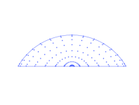
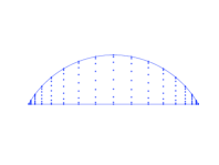
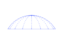
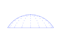
Figure 1: Four blending polynomial meshes for degree $n=4$ on a circular segment with angle $2\pi/3$, $m=2$ and $c=2\sqrt{2}$; the mesh cardinality is $9\times 17$ (top-left, top-right and bottom-left) and $9\times 9$ (bottom-right).

The corresponding polynomial meshes

$$\mathcal{A}_{n}(m)=\sigma\left(X_{mn}([0,1])\times W_{mn}([\omega_{1},\omega_{2}])\right)\;,$$ (22)

are optimal, since $d_{1}+d_{2}+d_{3}=2$ and $N=dim(\mathbb{P}_{n}^{2}(K))=(n+1)(n+2)/2\sim n^{2}/2$ (cf. Remark 1), with $c=\alpha\beta$.

A special role is played by planar circular lunes (difference of a disk with a second overlapping disk), that do not fall in the arc blending class and correspond to a transformation $\sigma$ where two angular variables are involved. Indeed a lune of the unit disk, whose boundary is given by two circular arcs, a longer one with semiangle say $\omega_{2}$ and a shorter one with semiangle say $\omega_{1}$, can be described by the bilinear trigonometric transformation $\sigma=(\sigma_{1},\sigma_{2})$

$$\sigma_{1}(\theta_{1},\theta_{2})=\cos(\theta_{2})-\frac{\cos(\omega_{1})}{\sin(\omega_{1})}\,\sin(\theta_{2})+\frac{1}{\sin(\omega_{1})}\,\cos(\theta_{1})\sin(\theta_{2})\;,$$

$$\sigma_{2}(\theta_{1},\theta_{2})=\frac{1}{\sin(\omega_{1})}\,\cos(\theta_{1})\sin(\theta_{2})\;,\;\;(\theta_{1},\theta_{2})\in[-\omega_{1},\omega_{1}]\times[0,\omega_{2}]\;.$$ (23)

As proved in [12] such a transformation maps (not injectively since $\sigma_{1}(\theta_{1},0)\equiv 1$) the boundary of the rectangle onto the boundary of the lune (preserving the orientation) and has positive Jacobian, so that it is a diffeomorphism of the interior of the rectangle onto the interior of the lune. Observe that (23) fall into the class (6) with $d=2$, $d_{1}=d_{2}=0$, $d_{3}=2$. The corresponding polynomial meshes

$$\mathcal{A}_{n}(m)=\sigma\left(W_{mn}([-\omega_{1},\omega_{1}])\times W_{mn}([0,\omega_{2}])\right)\;,$$ (24)

are again optimal, with $c=\beta^{2}$.

2.2 Sections of sphere and torus

The relevant transformation $\sigma$ has the form (9), which characterizes suitable arcwise sections of the sphere ($R=0$) or of the torus ($R>0$). In this surface instances we have $d_{1}=0$ (only angular coordinates are involved). As observed above, a spherical or toroidal rectangle corresponds to $d_{2}=0$, $d_{3}=2$, $\theta\in[\omega_{1},\omega_{2}]\times[\omega_{3},\omega_{4}]$, where $\omega_{2}-\omega_{1},\omega_{4}-\omega_{3}>0$, $[\omega_{1},\omega_{2}]\subseteq[-\pi/2,\pi/2]$ and $[\omega_{3},\omega_{4}]\subset[-\pi,\pi]$. The special case $[\omega_{1},\omega_{2}]=[-\pi/2,\pi/2]$ is a so-called spherical lune.

Special instances may be periodic in one of the variables. For example, a spherical collar corresponds to $d_{2}=d_{3}=1$, $[\omega_{3},\omega_{4}]=[-\pi,\pi]$ (the whole longitude range). Geometrically it is the portion of sphere between two parallel cutting planes.

The same holds for a spherical cap, one of the two portions of a sphere cut by a plane. Focusing on a polar cap (up to a rotation) we have now $[\omega_{1},\omega_{2}]=[\frac{\pi}{2}-\omega,\frac{\pi}{2}+\omega]$ with $\omega\leq\pi/2$ (the latter is a generalization of the usual latitude).

For $R>0$ and the same angular intervals we obtain what we may call a toroidal collar and a toroidal cap (geometrically, we are cutting a standard torus by planes parallel to the $x_{1}x_{2}$-plane).

On the other hand, for $[\omega_{3},\omega_{4}]\subset[-\pi,\pi]$ and $[\omega_{1},\omega_{2}]=[-\pi,\pi]$ we get a (surface) toroidal slice (we are cutting the torus by two half-planes hinged on the $x_{3}$-axis).

All the corresponding polynomial meshes

$$\mathcal{A}_{n}(m)=\sigma\left(W_{mn}([\omega_{1},\omega_{2}])\times W_{mn}([\omega_{3},\omega_{4}])\right)\;,$$ (25)

are optimal, with $c=\beta^{2}$ (or $c=\alpha\beta$ in periodic instances in one of the variables). In fact, $d_{1}+d_{2}+d_{3}=2$ and $N=dim(\mathbb{P}_{n}^{3}(K))\sim\gamma n^{2}$, specifically $N=(n+1)^{2}$ (sphere) or $N=2n^{2}$ (torus); cf. Remark 1. More generally, if $K$ is a polynomial determining compact subset of a real algebraic variety $\mathcal{M}\subset\mathbb{R}^{d}$ defined as the zero set of an irreducible real polynomial of degree $k$, then

$$N=dim(\mathbb{P}_{n}^{d}(K))=dim(\mathbb{P}_{n}^{d}(\mathcal{M}))={n+d\choose d}-{n-k+d\choose d}\;,$$ (26)

for $n\geq k$, and thus $N\sim\frac{k}{(d-1)!}\,n^{d-1}$ for $n\to\infty$ ($d$ and $k$ fixed). Indeed, the sphere is a quadric ($k=2$) whereas the torus is a quartic ($k=4$) surface in $d=3$ variables; see, e.g., [8] for the relevant algebraic geometry notions.

In Figure 2 we show two examples of surface optimal polynomial meshes on sections of sphere and torus. The numerical codes that generate the optimal polynomial meshes are available at [26].

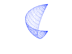
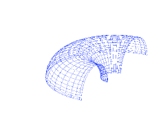
Figure 2: Optimal polynomial meshes (bullets) for $n=4$ with $m=3$ on a spherical lune (left) and a toroidal cap section (right).

2.3 Sections of ball and solid torus

We focus now on solid arcwise sections of ball and torus. A first class of sections corresponds to a rotation of planar sections around a coplanar axis, by an angle possibly smaller than $2\pi$. Such “solids of rotation”, together with the corresponding polynomial meshes, can be conveniently described using generalized cylindrical coordinates

$$x=(x_{1},x_{2},x_{3})=(r\cos(\phi),r\sin(\phi),z)\;,$$ (27)

where we have taken with no loss of generality the $x_{3}$-axis as the rotation axis, we have named for convenience $\phi$ the rotation angle, $z$ the $x_{3}$ coordinate and $r$ assumes also negative values (namely $(r,\phi)$ are generalized polar coordinates in planes orthogonal to the rotation axis). Rotation of planar bodies around a coplanar axis was studied also in [13], where however only the case of an external axis (standard cylindrical coordinates) was considered. By using generalized cylindrical coordinates the rotation axis can intersect the interior of the body (a planar disk section here).

Now, if the rotated planar domain, say $D$, is a blending domain (see Section 2.1), then $r=r(t,\theta)$, $z=z(t,\theta)$ have the form (20), so that $r,z\in\mathbb{P}_{1}([0,1])\bigotimes\mathbb{T}_{1}([\omega_{1},\omega_{2}])$, and the transformation $\sigma$ takes on the form

$$\sigma(t,\theta,\phi)=(r(t,\theta)\cos(\phi),r(t,\theta)\sin(\phi),z(t,\theta))\;,$$ (28)

where $(t,\theta,\phi)\in[0,1]\times[\omega_{1},\omega_{2}]\times[\phi_{1},\phi_{2}]$, which clearly falls in the class of Proposition 1.

This allows to construct optimal polynomial meshes on several arcwise solid sections, for example solid caps (one of the two portions of a ball cut by a plane), and spherical zones (the portion of a ball between two parallel cutting planes), that correspond to a complete rotation (i.e., by a multiple of $\pi$) of a planar circular segment or zone, respectively, around their symmetry axis.

A rotation of a half-disk around the diameter by an angle smaller than $2\pi$ produces a spherical slice (whose external boundary is a spherical lune).

A spherical cone corresponds to a complete rotation of a planar circular sector around its axis, whereas a spherical lens (the intersection of two overlapping balls) to a complete rotation of a planar lens (around the axis connecting the centers), and a spherical shell to a complete rotation of a disk annulus around a diameter.

Similarly, a complete rotation of circular segments and zones around an external axis parallel to their symmetry axis produce solid toroidal caps and zones, respectively (whose external boundaries are surface toroidal caps and collars).

If the entire disk is rotated around an external axis by an angle smaller than $2\pi$, we get a solid toroidal slice (whose external boundary is a surface toroidal slice).

In all the cases above the corresponding polynomial meshes

$$\mathcal{A}_{n}(m)=\sigma\left(X_{mn}([0,1])\times W_{mn}([\omega_{1},\omega_{2}])\times W_{mn}([\phi_{1},\phi_{2}])\right)\;,$$ (29)

are optimal, with $c=\alpha^{2}\beta$, except for the spherical shell where we can take $[\omega_{1},\omega_{2}]=[\phi_{1},\phi_{2}]=[0,2\pi]$ and thus $c=\alpha^{3}$. In fact, $d_{1}+d_{2}+d_{3}=3$ and $N=dim(\mathbb{P}_{n}^{3}(K))=(n+1)(n+2)(n+3)/6\sim n^{3}/6$.

If the rotated planar domain $D$ is a lune, then $r=r(\theta_{1},\theta_{2})$ and $z=z(\theta_{1},\theta_{2})$ have the form (23), so that $r,z\in\mathbb{T}_{1}([\omega_{1},\omega_{2}])\bigotimes\mathbb{T}_{1}([\omega_{3},\omega_{4}])$, and the transformation becomes

$$\sigma(\theta_{1},\theta_{2},\phi)=(r(\theta_{1},\theta_{2})\cos(\phi),r(\theta_{1},\theta_{2})\sin(\phi),z(\theta_{1},\theta_{2}))\;,$$ (30)

where $(\theta_{1},\theta_{2},\phi)\in[\omega_{1},\omega_{2}]\times[\omega_{3},\omega_{4}]\times[\phi_{1},\phi_{2}]$ are all angular variables. In case the rotation axis is the line connecting the two centers, we get a solid lune (the difference of a ball with a second overlapping ball). The optimal polynomial mesh is

$$\mathcal{A}_{n}(m)=\sigma\left(W_{mn}([\omega_{1},\omega_{2}])\times W_{mn}([\omega_{3},\omega_{4}])\times W_{mn}([\phi_{1},\phi_{2}])\right)\;,$$ (31)

with $c=\beta^{3}$.

A different situation, not of rotation type, arises when we consider a spherical square pyramid, that is a pyramid whose base is a geographic rectangle (the region of sphere comprised between two given latitudes and longitudes) and whose vertex, say $V=(v_{1},v_{2},v_{3})$, lies inside the ball. In this case, we can take the degenerate trivariate blending transformation

$$\sigma(t,\theta_{1},\theta_{2})=t\left(\cos(\theta_{1})\cos(\theta_{2}),\cos(\theta_{1})\sin(\theta_{2}),\sin(\theta_{1})\right)+(1-t)V\;,$$ (32)

where $(t,\theta_{1},\theta_{2})\in[0,1]\times[\omega_{1},\omega_{2}]\times[\omega_{3},\omega_{4}]$. The optimal polynomial mesh has the form (29) with $c=\alpha\beta^{2}$.

In Table 1, we have listed (with no pretence of exhaustivity) the planar, surface and solid cases discussed above, together with the corresponding mesh parameters.

Table 1: Some standard planar, surface and solid sections together with the corresponding polynomial mesh parameters (cf. Proposition 1).

$c$	card. bound	section type
$\alpha$	$N_{2}$	entire circle
$\beta$	$N_{2}$	circle arc
$\alpha^{2}$	$N_{1}N_{2}$	entire disk/disk annulus
	$N_{2}^{2}$	entire sphere/torus
$\alpha\beta$	$N_{1}N_{2}$	disk sector/segment/zone/lens
		surface spherical cap/collar
		surface toroidal cap/collar/slice
$\beta^{2}$	$N_{2}^{2}$	planar lune
		surface spherical rectangle/lune
		surface toroidal rectangle
$\alpha^{3}$	$N_{1}N_{2}^{2}$	entire ball/solid torus
		spherical shell
$\alpha^{2}\beta$	$N_{1}N_{2}^{2}$	solid spherical cap/cone/lens/zone
		solid toroidal cap/slice/zone
$\alpha\beta^{2}$	$N_{1}N_{2}^{2}$	spherical square pyramid
$\beta^{3}$	$N_{2}^{3}$	solid lune

References

• [1] B. Adcock, D. Huybrechs and J.M. Vaquero, On the numerical stability of Fourier extensions, Found. Comput. Math. 14 (2014), 635–687.
• [2] L. Bos, J.P. Calvi, N. Levenberg, A. Sommariva and M. Vianello, Geometric Weakly Admissible Meshes, Discrete Least Squares Approximation and Approximate Fekete Points, Math. Comp. 80 (2011), 1601–1621.
• [3] L. Bos, S. De Marchi, A. Sommariva and M. Vianello, Computing multivariate Fekete and Leja points by numerical linear algebra, SIAM J. Numer. Anal. 48 (2010), 1984–1999.
• [4] L. Bos and M. Vianello, Low cardinality admissible meshes on quadrangles, triangles and disks, Math. Inequal. Appl. 15 (2012), 229–235.
• [5] L. Bos and M. Vianello, Subperiodic trigonometric interpolation and quadrature, Appl. Math. Comput. 218 (2012), 10630–10638.
• [6] J.P. Calvi and L. Bialas-Ciez, Invariance of polynomial inequalities under polynomial maps, J. Math. Anal. Appl. 439 (2016), 449–464.
• [7] J.P. Calvi and N. Levenberg, Uniform approximation by discrete least squares polynomials, J. Approx. Theory 152 (2008), 82–100.
• [8] D.A. Cox, J. Little and D. O’Shea, Ideals, varieties, and algorithms, fourth edition, Springer, 2015.
• [9] G. Da Fies, A. Sommariva and M. Vianello, Algebraic cubature by linear blending of elliptical arcs, Appl. Numer. Math. 74 (2013), 49–61.
• [10] G. Da Fies and M. Vianello, Trigonometric Gaussian quadrature on subintervals of the period, Electron. Trans. Numer. Anal. 39 (2012), 102–112.
• [11] G. Da Fies and M. Vianello, On the Lebesgue constant of subperiodic trigonometric interpolation, J. Approx. Theory 167 (2013), 59–64.
• [12] G. Da Fies and M. Vianello, Product Gaussian quadrature on circular lunes, Numer. Math. Theory Methods Appl. 7 (2014), 251–264.
• [13] S. De Marchi and M. Vianello, Polynomial approximation on pyramids, cones and solids of rotation, Dolomites Res. Notes Approx. DRNA 6 (2013), 20–26.
• [14] H. Ehlich and K. Zeller, Schwankung von Polynomen zwischen Gitter punkten, Math. Z. 86 (1964), 41–44.
• [15] M. Gentile, A. Sommariva and M. Vianello, Polynomial approximation and quadrature on geographic rectangles, Appl. Math. Comput. 297 (2017), 159–179.
• [16] K. Jetter, J. Stökler and J.D. Ward, Norming sets and spherical cubature formulas, Advances in computational mathematics (Guangzhou, 1997), 237–244, Lecture Notes in Pure and Appl. Math., 202, Dekker, New York, 1999.
• [17] A. Kroó, On optimal polynomial meshes, J. Approx. Theory 163 (2011), 1107–1124.
• [18] A. Kroó, On the existence of optimal meshes in every convex domain on the plane, J. Approx. Theory, available online 15 March 2017.
• [19] P. Leopardi, A. Sommariva and M. Vianello, Optimal polynomial meshes and Caratheodory-Tchakaloff submeshes on the sphere, Dolomites Res. Notes Approx. DRNA 10 (2017), 18–24 .
• [20] F. Piazzon, Optimal polynomial admissible meshes on some classes of compact subsets of $\mathbb{R}^{d}$, J. Approx. Theory 207 (2016), 241–264.
• [21] F. Piazzon, Pluripotential Numerics, arXiv preprint 1704.03411, April 2017.
• [22] F. Piazzon and M. Vianello, Small perturbations of polynomial meshes, Appl. Anal. 92 (2013), 1063–1073.
• [23] F. Piazzon and M. Vianello, Jacobi norming meshes, Math. Inequal. Appl. 19 (2016), 1089–1095.
• [24] F. Piazzon and M. Vianello, A note on total degree polynomial optimization by Chebyshev grids, Optim. Lett. 12 (2018), 63–71.
• [25] A. Sommariva and M. Vianello, Polynomial fitting and interpolation on circular sections, Appl. Math. Comput. 258 (2015), 410–424.
• [26] A. Sommariva and M. Vianello, Matlab codes for the computation of planar, surface and solid polynomial meshes, available online at
http://www.math.unipd.it/~alvise/software.html.
• [27] M. Vianello, Norming meshes by Bernstein-like inequalities, Math. Inequal. Appl. 17 (2014), 929–936.
• [28] M. Vianello, Global polynomial optimization by norming meshes on sphere and torus, submitted for publication, available online at:
http://www.math.unipd.it/~marcov/publications.html.