Abstract

A general form of the octupole collective Hamiltonian is introduced and analyzed based on fundamental tensors in the seven-dimensional tensor space. Possible definitions of intrinsic frames of reference possessing cubic symmetry for the octupole tensor are considered. Cubic intrinsic octupole coordinates or deformations are introduced. Shapes of the octupoloid are investigated. The octupole collective Hamiltonian is expressed in intrinsic coordinates. An intrinsic angular momentum carried by the octupole vibrations is discovered. Small oscillations about an axially-symmetric pear shape are analyzed. Formulation of a unified quadrupole-octupole collective model is discussed.

Chapter 0 The octupole collective Hamiltonian.
Does it follow the example of the quadrupole case?

1 Introduction

The idea of attributing a definite multipolarity to nuclear collective excitations came from the nuclear liquid-drop model. It was known before the discovery of atomic nuclei that the normal modes of the surface vibrations of a spherical drop of incompressible liquid have definite multipolarities [1]. Many years later, when atomic nuclei were already known, Siegfried Flügge [2] connected the eigenfrequencies of the surface vibrations of a nuclear liquid drop with the excitation energies of low-lying states of even-even nuclei. These were the beginnings of the collective model.

The most important collective mode in nuclear structure physics is that with multipolarity $\lambda=2$, because it concerns the lowest excited states in even-even nuclei. These states are well known experimentally and theoretical methods describing them are well developed. One such method, applicable to even-even nuclei only, is a description by means of the Schrödinger equation in a collective space. Initiated by Aage Bohr [3] a long time ago, it is very effective and is still in use. The Bohr Hamiltonian became the label of the model. When applying the method one usually starts with a general classical collective Hamiltonian [4, 5]. Its form has been extracted from various microscopic many-body models through methods of the “Adiabatic Time-Dependent Hartree-Fock-Bogolyubov” (ATDHFB) type (see e.g. Chapt. 12 in Ref.[6]) and then quantized by means of the Podolsky-Pauli prescription [7, 8, 9]. Such a quasi-classical approach is still used even today. It would be good to use purely quantum methods to describe the collective states. Therefore, the Generator Coordinate Method (GCM) has been recently employed [10, 11]. It leads to integral equations instead of differential ones (see e.g. Chapt. 10 in Ref.[6]). However, in an approximation to the GCM called the Gaussian Overlap Approximation (GOA) the Hill-Wheeler integral equations for collective motion can be reduced back to differential equations with a collective Hamiltonian [12].

Apart from the positive-parity quadrupole states, negative-parity levels have been observed for a long time [13] in the low-energy spectra of even-even nuclei. Multipolarity $\lambda=3$ has been attributed to such states. Information on the octupole states has been collected over many years, see Refs. [14] and [15] for reviews. Recently, measurements of a static octupole deformation in radium (²²⁴Ra) and barium (¹⁴⁴Ba) isotopes have been reported [16, 17]. However, data on the octupole states are not so rich as in the case of quadrupole excitations. This is perhaps connected with experimental and interpretational difficulties. A common opinion seems to be that the quadrupole collective Hamiltonian stands for a pattern for higher multipolarities. However, it is not so easy. The theory of the octupole degrees of freedom is much more complicated than that of the quadrupole ones, or rather the quadrupole case is exceptionally simple. This will be demonstrated further in subsequent Sections. In GCH a general form of the octupole collective Hamiltonian is introduced and discussed in comparison with that of the quadrupole one. Possible definitions of intrinsic frames of reference for the octupole tensor in analogy to that for the quadrupole tensor are considered in IF. The octupole deformation parameters are introduced and illustrated. The octupole Hamiltonian is expressed in intrinsic coordinates in IHAM. Its approximate form for small oscillations around a pear shape is given in AS. In Conclusion, in CONCL, a draft of a unified quadrupole-octupole collective model is recapitulated.

2 General form of collective Hamiltonians

The idea of collective models consists generally in describing some complex (collective) states of a many-body system through the substitution of the coordinates of many particles by a relatively small number of collective variables. An appropriate choice of these collective variables decides the success of the model. Constructing the collective models in question here for the description of low-lying collective states of even-even nuclei one takes the spherical tensors $\boldsymbol{\alpha}_{\lambda}$ as collective variables. These tensors are transformed according to irreducible $(2\lambda+1)$-dimensional representations D^λ of the O(3) group of orthogonal transformations in the physical space. The spherical components $\alpha_{\lambda\mu}$ ($\mu=-\lambda,\dots,\lambda$) of $\boldsymbol{\alpha}_{\lambda}$ in the laboratory frame, U_lab, are the collective laboratory coordinates. It is assumed that the tensor $\boldsymbol{\alpha}_{\lambda}$ is electric i.e. has parity $(-1)^{\lambda}$ and real, which means that its components fulfill the relation $\alpha^{*}_{\lambda\mu}=(-1)^{\mu}\alpha_{\lambda-\mu}$. The differential operators $-i\partial/\partial\alpha^{*}_{\lambda\mu}$ play the role of the momenta canonically conjugate to the coordinates $\alpha_{\lambda\mu}$. The angular momentum operators or the O(3) generators in the collective space fulfill characteristic commutation relations with the coordinates and momenta (see e.g. Appendix A.1. in Ref. [18]). The following vector operator:

$$L^{(\lambda)}_{1\mu}(\boldsymbol{\alpha}_{\lambda})=(-1)^{\lambda}\sqrt{\frac{\lambda(\lambda+1)(2\lambda+1)}{3}}\sum_{\kappa\nu}(\lambda\kappa\lambda\nu|1\mu)\alpha_{\lambda\kappa}\frac{\partial}{\partial\alpha^{*}_{\lambda\nu}}$$ (1)

fulfills such commutation relations and thus plays the role of the collective angular momentum [18, 19].

The nuclear collective system is defined by a collective Hamiltonian $H_{\lambda}(\boldsymbol{\alpha}_{\lambda})$. It is assumed that $H_{\lambda}(\boldsymbol{\alpha}_{\lambda})$ has the following properties:

It is a second-order differential operator (like the Schrödinger operator),

it is real, i.e. $H_{\lambda}(\boldsymbol{\alpha}_{\lambda})=H^{*}_{\lambda}(\boldsymbol{\alpha}_{\lambda})$ (it describes even-even nuclei only),

it is a scalar with respect to the orthogonal group O(3) (rotations and inversion in the physical space) or commutes with the angular momentum operators of angmom,

it is Hermitian with a scalar weight $W(\boldsymbol{\alpha}_{\lambda})\geq 0$,

it possesses the lowest eigenvalue (positive kinetic energy),

it is an isotropic function of the coordinates, i.e. it does not depend on any other tensor quantities. No other assumptions are needed at this stage (cf. Ref. [20]). The most general form of $H_{\lambda}(\boldsymbol{\alpha}_{\lambda})$ with properties (1) – (6) given above reads [18, 12]:

$$H_{\lambda}(\boldsymbol{\alpha}_{\lambda})=-\frac{1}{2W(\boldsymbol{\alpha}_{\lambda})}\sum_{\mu,\nu}\frac{\partial}{\partial\alpha_{\lambda\mu}}W(\boldsymbol{\alpha}_{\lambda})B^{-1}_{\lambda\mu\lambda\nu}(\boldsymbol{\alpha}_{\lambda})\frac{\partial}{\partial\alpha_{\lambda\nu}}+V(\boldsymbol{\alpha}_{\lambda}),$$ (2)

The Hamiltonian is determined by three quantities: two real scalar functions — weight $W(\boldsymbol{\alpha}_{\lambda})$ and potential $V(\boldsymbol{\alpha}_{\lambda})$, and a symmetric $(2\lambda+1)\times(2\lambda+1)$ matrix of real so-called inverse inertial functions $B^{-1}_{\lambda\mu\lambda\nu}(\boldsymbol{\alpha}_{\lambda})$. Since the matrix is transformed under the O(3) group like a product of two tensors $\boldsymbol{\alpha}_{\lambda}$ it is called a symmetric bitensor. All these three quantities depend on no other tensors but $\boldsymbol{\alpha}_{\lambda}$ and therefore they are isotropic tensor fields in the $(2\lambda+1)$-dimensional collective space. They can either be calculated from microscopic many-body models or fitted to experimental data. When the Hamiltonian is obtained by quantization of its classical counterpart the weight is $W(\boldsymbol{\alpha}_{\lambda})=\sqrt{\det{B_{\lambda\mu\lambda\nu}(\boldsymbol{\alpha}_{\lambda})}}$.

In order to investigate possible structures of the inverse inertial bitensor it is convenient to express it as a set of (single) tensors $\boldsymbol{T}_{2l}(\boldsymbol{\alpha}_{\lambda})$ ($l=0,\dots,\lambda$), namely

$$B^{-1}_{\lambda\mu\lambda\nu}(\boldsymbol{\alpha}_{\lambda})=\sum_{l=0}^{\lambda}(\lambda\mu\lambda\nu|2l\ m)T_{2l\ m}(\boldsymbol{\alpha}_{\lambda})$$ (3)

Assumption (6), that the $\boldsymbol{T}_{2l}(\boldsymbol{\alpha}_{\lambda})$ are isotropic functions of $\boldsymbol{\alpha}_{\lambda}$ is essential here. Then, an arbitrary tensor $\boldsymbol{T}_{\Lambda}(\boldsymbol{\alpha}_{\lambda})$ can be expressed in the following form:

$$\boldsymbol{T}_{\Lambda}(\boldsymbol{\alpha}_{\lambda})=\sum_{k=1}^{k_{\lambda\Lambda}}\sigma^{(\Lambda)}_{k}(\boldsymbol{\alpha}_{\lambda})\boldsymbol{\tau}_{k\Lambda}(\boldsymbol{\alpha}_{\lambda})$$ (4)

by a number of definite fundamental tensors $\boldsymbol{\tau}_{k\Lambda}(\boldsymbol{\alpha}_{\lambda})$ for given $\lambda$ and $\Lambda$, and arbitrary scalar coefficients $\sigma^{(\Lambda)}_{k}(\boldsymbol{\alpha}_{\lambda})$ (see Appendix A in Ref. [18]). The original Bohr inverse inertial bitensor [3] has the following form:

$$B^{-1}_{\lambda\mu\lambda\nu}(\boldsymbol{\alpha}_{\lambda})=(\lambda\mu\lambda\nu|00)(-1)^{\lambda}\sqrt{2\lambda+1}\frac{1}{B_{\lambda}}=\frac{(-1)^{\mu}\delta_{\mu-\nu}}{B_{\lambda}}$$ (5)

where $B_{\lambda}$ is a constant mass parameter.

In the case of a general quadrupole $(\lambda=2)$ collective Hamiltonian it is well known that the inverse inertial bitensor can have at most six independent components out of fifteen possible ones [5, 18]. It is interesting to know whether there are similar restrictions for the components of the inverse inertial bitensor in the case of an octupole $(\lambda=3)$ collective Hamiltonian. Unfortunately, the things are much more complicated in that case. The symmetric bitensor $B^{-1}_{3\mu 3\nu}(\boldsymbol{\alpha}_{3})$ has twenty-eight components. Can they all be independent? To answer this question one should analyze Eqs. (3) and (4) for $\lambda=3$.

According to bll the even (positive-parity) symmetric octupole bitensor, $B^{-1}_{3\mu 3\nu}(\boldsymbol{\alpha}_{3})$, can be replaced with four tensors $\boldsymbol{T}_{2l}(\boldsymbol{\alpha}_{3})$ ( $l=0,\dots,3$). These tensors should be even isotropic functions of $\boldsymbol{\alpha}_{3}$. The tensor fields in the space of the octupole coordinates are built out of some twenty-six elementary tensors

$$\boldsymbol{t}^{(n)}_{l}=[\underbrace{\boldsymbol{\alpha}_{3}\times\ \dots\ \times\boldsymbol{\alpha}_{3}}_{n}]_{l}$$ (6)

(square brackets $[\dots]_{l}$ stand for vector coupling to rank $l$) for $l<3n$ and related to each other by about two hundred syzygies or relations in the form of rational integral functions [21]. All the elementary tensors split into two groups with positive and negative spin-parity $(-1)^{l+n}$, respectively. Independent fundamental tensors $\boldsymbol{\tau}_{k\Lambda}(\boldsymbol{\alpha}_{3})$ from tstau are constructed by alignment of the elementary tensors of elten. The positive spin-parity elementary and even (positive parity) fundamental tensors needed to construct the inverse inertial bitensor in question are listed in ET. There are twenty-eight relevant fundamental tensors altogether and thus, all twenty-eight components of the bitensor $B^{-1}_{3\mu 3\nu}(\boldsymbol{\alpha}_{3})$ can be arbitrary tensor fields in the octupole collective space. No additional relations between the components need appear. Twenty-eight scalars $\sigma^{(\Lambda)}_{k}(\boldsymbol{\alpha}_{3})$ for $k=1,\dots,k_{3\Lambda}$ and $\Lambda=0,\ 2,\ 4,\ 6$ are functions of the four elementary scalars, eet.

3 Intrinsic frame and intrinsic coordinates

1 Intrinsic frames of reference

Obviously, the tensor $\boldsymbol{\alpha}_{\lambda}$ can be represented by different sets of coordinates in different frames of reference. As already stated in GCH, the $\alpha_{\lambda\mu}$ are the components of $\boldsymbol{\alpha}_{\lambda}$ in the frame U_lab. Let us take another frame, say U_in, the orientation of which with respect to the laboratory frame U_lab is given by the Euler angles $\omega=(\varphi,\vartheta,\psi)$. We will not use the spherical components of $\boldsymbol{\alpha}_{\lambda}$ in the frame U_in. Instead, we shall use their real and imaginary parts, $a_{\lambda k}$ and $b_{\lambda k}$, respectively, defined in the standard way (cf e.g. Eq. A.7 in Ref. [18]). Then, the transformation rule between the corresponding components of the tensor $\boldsymbol{\alpha}_{\lambda}$ with respect to U_lab and U_in, respectively, takes the following form (cf. Ref. [19]):

$$\alpha_{\lambda\mu}=D^{\lambda(+)}_{\mu 0}(\omega)a_{\lambda 0}+\sum_{k=1,2,3}[D^{\lambda(+)}_{\mu k}(\omega)a_{\lambda k}+D^{\lambda(-)}_{\mu k}(\omega)b_{\lambda k}]$$ (7)

where

$$D^{\lambda(+)}_{\mu k}(\omega)=\frac{1}{\sqrt{2(1+\delta_{k0}{)}}}[\mathcal{D}^{\lambda}_{\mu k}(\omega)+(-1)^{k}\mathcal{D}^{\lambda}_{\mu-k}(\omega)]$$

$$D^{\lambda(-)}_{\mu k}(\omega)=\frac{i}{\sqrt{2}}[\mathcal{D}^{\lambda}_{\mu k}(\omega)-(-1)^{k}\mathcal{D}^{\lambda}_{\mu-k}(\omega)]$$ (8)

are the semi-Cartesian Wigner functions. The Bohr-Mottelson definition of the Wigner functions, $\mathcal{D}^{\lambda}_{\mu k}(\omega)$, is used [22].

For the frame U_in to be the intrinsic frame, three properly chosen conditions for the coordinates $a_{\lambda k}$ and $b_{\lambda k}$ should be given, namely

$$\Omega_{i}(a_{\lambda k}(\omega,\alpha_{\lambda\mu}),b_{\lambda k}(\omega,\alpha_{\lambda\mu}))=\Omega_{i}(\omega,\alpha_{\lambda\mu})=0$$ (9)

for $i=1,\ 2,\ 3$, which determine the three Euler angles, $\omega=(\varphi,\vartheta,\psi)$ as functions of the laboratory coordinates and, in this way, impart the status of intrinsic coordinates to them. The remaining $2\lambda-2$ independent coordinates are usually called deformations.

The concept of an intrinsic (body-fixed) frame of reference is connected with the descriptions of collective states from the very beginning [3]. The principal axes of the tensor $\boldsymbol{\alpha}_{2}$ are taken as the intrinsic axes in the quadrupole, $\lambda=2$, case. According to cc2 from Appendix 0.D the well-known definition of the intrinsic frame is $g_{2s}=0$ for $s=x,y,z$. It is seen from Appendix 0.B that the frame U_in is then O_h-symmetric. The two remaining intrinsic coordinates, $a_{20}=\beta\cos{\gamma}$ and $a_{22}=\beta\sin{\gamma}$, are usually parametrized by the well-known deformation parameters $\beta$ and $\gamma$.

The problem of the intrinsic frame for the octupole tensor, $\boldsymbol{\alpha}_{3}$, has appeared to be less transparent than that for $\lambda=2$. The tensor has no principal axes and thus no obvious intrinsic frame. Early attempts to define an intrinsic frame failed (cf Ref. [23]). This was, perhaps, the reason why the intrinsic frame of reference was for a long time determined with the quadrupole tensor and octupole coordinates were treated as intrinsic coordinates with respect to that frame (cf. Ref.  [19]). And what shall we do when any quadrupole tensor is not at our disposal?

In order to define an intrinsic frame for $\lambda=3$, having the natural symmetry O_h, it is convenient to decompose the tensor representation D³ of the O(3) group onto the O_h irreps A${}^{-}_{2}$, F${}^{-}_{1}$ and F${}^{-}_{2}$, respectively (see Appendix 0.C). The corresponding representations will be called the octupole cubic Wigner functions $A_{\mu}(\omega)$, $F_{\mu s}(\omega),\ (s=x,y,z)$ and $G_{\mu s}(\omega),\ (s=x,y,z)$, respectively. They are the following combinations of the semi-Cartesian Wigner functions:

$$A_{\mu}(\omega)=D^{3(-)}_{\mu 2}(\omega)$$

$$F_{\mu x}(\omega)=\sqrt{\frac{3}{8}}D^{3(+)}_{\mu 1}(\omega)-\sqrt{\frac{5}{8}}D^{3(+)}_{\mu 3}(\omega),$$

$$F_{\mu y}(\omega)=\sqrt{\frac{3}{8}}D^{3(-)}_{\mu 1}(\omega)+\sqrt{\frac{5}{8}}D^{3(-)}_{\mu 3}(\omega),$$

$$F_{\mu z}(\omega)=D^{3(+)}_{\mu 0}(\omega)$$

$$G_{\mu x}(\omega)=\sqrt{\frac{5}{8}}D^{3(+)}_{\mu 1}(\omega)+\sqrt{\frac{3}{8}}D^{3(+)}_{\mu 3}(\omega)$$

$$G_{\mu y}(\omega)=-\sqrt{\frac{5}{8}}D^{3(-)}_{\mu 1}(\omega)+\sqrt{\frac{3}{8}}D^{3(-)}_{\mu 3}(\omega)$$

$$G_{\mu z}(\omega)=D^{3(+)}_{\mu 2}(\omega).$$ (10)

The cubic Wigner functions form a unitary set. When using them the transformation rule of retr takes the following form:

$$\alpha_{3\mu}(\omega,b,f)=A_{\mu}(\omega)b+\sum_{s=x,y,z}[F_{\mu s}(\omega)f_{s}+G_{\mu s}(\omega)g_{s}]$$ (11)

where $b$, $f_{s}$ and $g_{s}$ are the octupole cubic coordinates in the frame U_in, proposed in Ref. [24] and defined in Appendix 0.D.

It is seen that we have two possible definitions of the O_h-symmetric frame of reference. We can take intr in the two following alternative forms: either $g_{s}=0$ or $f_{s}=0$ for $s=x,y,z$. Here, we shall explore the former definition. Both of them are briefly discussed in Ref. [25]. We see from labcub that in the former case the following relation between the spherical laboratory coordinates and the Euler angles and the octupole deformations holds:

$$\alpha_{3\mu}(\omega,b,f)=A_{\mu}(\omega)b+\sum_{s=x,y,z}F_{\mu s}(\omega)f_{s}$$ (12)

The Jacobian of the transformation $\alpha_{\mu}\to\omega,b,f_{s}$ is equal to

$$D_{f}(\vartheta,b,f_{x},f_{y},f_{z}) = 8\sin{\vartheta}\left[b\left(b^{2}-\frac{15}{16}\left(f_{x}^{2}+f_{y}^{2}+f_{z}^{2}\right)\right)+\frac{15}{8}\sqrt{\frac{15}{16}}f_{x}f_{y}f_{z}\right]$$ (13)

$$= 8\sin{\vartheta}d_{f}(b,f_{s})$$

The transformation (12) is reversible for the deformations contained aside from the hyper-surface $D_{f}(\vartheta,b,f_{x},f_{y},f_{z})=0$, where ambiguities appear arising from the symmetries of the shape. The F${}^{-}_{1}$-covariant (vector) deformations ($f_{x},f_{y},f_{z}$) are transformed under the O_h transformations of the intrinsic frame like the Cartesian coordinates $x,y,z$ of a position vector.

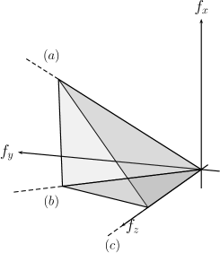
Figure 1: Infinite triangular pyramid mapping out the three-dimensional region of octupole vector deformations ($f_{x},f_{y},f_{z}$) with the vertex at point (0,0,0). The three pyramid edges are: (a) principal diagonal of octant $f_{x},f_{y},f_{z}\geq 0$, (b) diagonal of plane $f_{y}f_{z}$, (c) axis $f_{z}$.

It follows directly from the O_h symmetry that it is sufficient to consider, for instance, the region $0\leq f_{x}\leq f_{y}\leq f_{z}$ of vector deformations forming an infinite triangular pyramid in three-dimensional space (see fig_pyr). The forty-eight pyramids obtained by all the O_h transformations fill up the entire space. Deformation $b$ supplements the space of vector deformations to the four-dimensional space. It is invariant under rotations $R_{1}$ and $R_{3}$ and changes sign under $R_{2}$ and inversion $P$ together with the corresponding transformations of the vector deformations. Therefore, there are no additional restrictions on values of $b$ (see fig_pmbfz below). The case when $f_{x}^{2}+f_{y}^{2}+f_{z}^{2}=0$ is an exception: it is sufficient then to consider values $b\geq 0$.

To learn the geometrical meaning of the deformation parameters, $b$ and $f_{s}$, one can investigate the shapes of the “octupoloid” given by the following equation in the spherical coordinates $R$, $\theta$, $\phi$:

$$R(\theta,\phi)=R_{0}\left[1-A_{0}(\phi,\theta,0)b+\sum_{s=x,y,z}(1-2\delta_{sx})F_{0s}(\phi,\theta,0)f_{s}\right]$$ (14)

in accordance with the approach of Ref. [26], bearing in mind that $\mathcal{D}^{\lambda}_{0\mu}(\phi,\theta,0)=(-1)^{\mu}\sqrt{4\pi/(2\lambda+1)}Y_{\lambda\mu}(\theta,\phi)$. The shape of the octupoloid is defined by the set of deformations $b$, $f_{x}$, $f_{y}$ and $f_{z}$ up to the cubic group of transformations i.e. the Bohr rotations and mirror reflections (see Appendix 0.C).

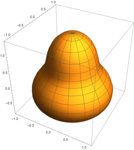
(a) $f_{z}=0.5,b=f_{x}=f_{y}=0$

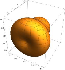
(b) $f_{y}=0.5,b=f_{x}=f_{z}=0$

Figure 2: Two octupoloids with identical axial-symmetric (pear) shapes oriented differently.

Two octupoloids with identical axial-symmetric (pear) shapes but oriented differently are shown in fig_fyz. Obviously, the two sets of vector deformations then lie inside different pyramids of fig_pyr. Changing the sign of the deformation gives inverted octupoloids with the same shape as that in the figure. Examples of octupoloids with asymmetric shapes are shown in fig_bfxyz. Their orientations and/or handedness can be changed by cubic group transormations of the deformations. For instance, changing the signs of all the deformations gives inverted octupoloids.

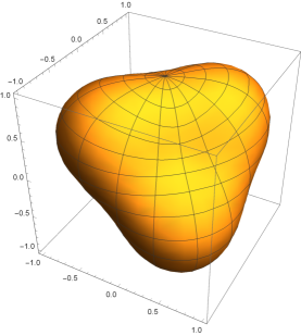
(a) $b=0.5,f_{x}=f_{y}=f_{z}=0$

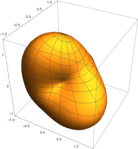
(b) $b=0.5,f_{z}=0.5,f_{y}=0.4,f_{x}=0.3$

Figure 3: Examples of octupoloids with asymmetric shapes.

However, when deformations belonging to one out of the two irreducible representations of the cubic group are transformed the shape of the octupoloid is changed, as shown in fig_pmbfz. Changing the sign of $b$ without changing the vector deformations gives a change of shape.

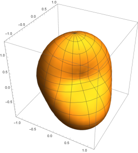
(a) $f_{z}=0.5,b=0.5,f_{x}=f_{y}=0$

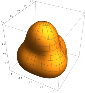
(b) $f_{z}=0.5,b=-0.5,f_{x}=f_{y}=0$

Figure 4: Two octupoloids with opposite signs of deformation $b$ having different shapes.

2 The Hamiltonian in intrinsic coordinates

A reversible transformation between the laboratory and intrinsic coordinates allows us to use interchangeably one or another set of variables. The use of intrinsic coordinates is usually more convenient because it gives the possibility to separate variables, especially the Euler angles. It is evident for potentials depending on the laboratory coordinates through the elementary scalars, the number of which coincides with the number of deformations. Hence, the potential in haml is a function of the number of deformation parameters characteristic for a given multipolarity: two for $\lambda=2$ and four for $\lambda=3$.

To express the kinetic part of the Hamiltonian and angular momenta in intrinsic coordinates we have to convert derivatives with respect to the laboratory coordinates into derivatives with respect to the intrinsic variables. As might be expected (cf. Ref. [27]), independently of the multipolarity of the collective space the components of the angular momentum of angmom can be expressed as

$$L^{(\lambda)}_{1\kappa}=D^{1(+)}_{\kappa 0}(\omega)L_{z}(\omega)-{D}^{1(+)}_{\kappa 1}(\omega)L_{x}(\omega)+{D}^{1(-)}_{\kappa 1}(\omega)L_{y}(\omega)$$ (15)

where $L_{x}$, $L_{y}$, $L_{z}$ are the Cartesian components of the intrinsic angular momentum depending on the Euler angles and their derivatives only and are given by the following standard formulae: (cf. e.g. Eq. (2.15) in Ref. [18]).

$${L}_{x}(\varphi,\vartheta,\psi) = -i\left(-\frac{\cos{\psi}}{\sin{\vartheta}}\frac{\partial}{\partial\varphi}+\sin{\psi}\frac{\partial}{\partial\vartheta}+\cot{\vartheta}\cos{\psi}\frac{\partial}{\partial\psi}\right)$$

$${L}_{y}(\varphi,\vartheta,\psi) = -i\left(\frac{\sin{\psi}}{\sin{\vartheta}}\frac{\partial}{\partial\varphi}+\cos{\psi}\frac{\partial}{\partial\vartheta}-\cot{\vartheta}\sin{\psi}\frac{\partial}{\partial\psi}\right)$$ (16)

$${L}_{z}(\varphi,\vartheta,\psi) = -i\frac{\partial}{\partial\psi}$$

For $\lambda=2$ the procedure for converting the derivatives is well known and is presented in detail, e.g., in Ref. [18]. A general quadrupole Hamiltonian expressed in intrinsic variables is divided into the vibrational part depending only on two deformations and the rotational Hamiltonian which contains the angular momenta $L_{x}$, $L_{y}$, $L_{z}$ and the deformation dependent moments of inertia. The intrinsic axes are always the principal axes of the tensor of inertia. When we take the kinetic energy with the Bohr inversed inertial bitensor (5) the structure of the Hamiltonian will not change much. Namely, the mixed term in the vibrational kinetic energy will vanish and the remaining five kinetic-energy terms — vibrational and rotational — contain one common constant mass parameter $B_{2}$ instead of different deformation-dependent inertial functions.

The procedure for transforming the octupole collective Hamiltonian to intrinsic coordinates is more involved than that for the case of $\lambda=2$. The first step of the procedure is conversion of the derivatives with respect to the laboratory coordinates into those with respect to the intrinsic variables. To do this one should calculate the derivatives of the intrinsic with respect to the laboratory coordinates. The transformation the reverse of that of intrtolabf can be presented in the following entangled form:

$$b=\sum_{\mu}(A_{\mu}(\omega))^{*}\alpha_{3\mu},$$

$$f_{s}=\sum_{\mu}(F_{\mu s}(\omega))^{*}\alpha_{3\mu}$$

$$0=\sum_{\mu}(G_{\mu s}(\omega))^{*}\alpha_{3\mu}$$ (17)

for $s=x,y,z$. Derivatives of deformations $b$ and $f_{s}$ with respect to the laboratory variables $\alpha_{3\mu}$ are equal to

$$\frac{\partial b}{\partial\alpha_{3\mu}}=(A_{\mu}(\omega))^{*}+\sum_{\nu,\omega}\frac{\partial}{\partial\omega}(A_{\nu}(\omega))^{*}\alpha_{3\nu}\frac{\partial\omega}{\partial\alpha_{3\mu}}$$

$$\frac{\partial f_{s}}{\partial\alpha_{3\mu}}=(F_{\mu s}(\omega))^{*}+\sum_{\nu,\omega}\frac{\partial}{\partial\omega}(F_{\nu s}(\omega))^{*}\alpha_{3\nu}\frac{\partial\omega}{\partial\alpha_{3\mu}}$$ (18)

Derivatives of the Euler angles with respect to $\alpha_{3\mu}$ are obtained by solving the following set of linear equations:

$$\sum_{\nu}\left[(\frac{\partial}{\partial\varphi}(G_{\nu s}(\omega))^{*})\frac{\partial\varphi}{\partial\alpha_{3\mu}}+(\frac{\partial}{\partial\vartheta}(G_{\nu s}(\omega))^{*})\frac{\partial\vartheta}{\partial\alpha_{3\mu}}+(\frac{\partial}{\partial\psi}(G_{\nu s}(\omega))^{*})\frac{\partial\psi}{\partial\alpha_{3\mu}}\right]\alpha_{3\nu}$$

$$+(G_{\mu s}(\omega))^{*}=0\qquad\mathrm{for}\quad s=x,y,z.$$ (19)

To calculate all the derivatives from Eqs. (2) and(2) one should calculate the derivatives of the octupole cubic Wigner functions with respect to the Euler angles. Using Eqs. (1) and (1) the derivatives of the cubic functions can be expressed by derivatives of the Wigner functions themselves. E.g., handbook [28] contains formulae for the derivatives in question and other relevant properties of the Wigner functions. Finally, solutions of eqforder for derivatives of the Euler angles with respect to $\alpha_{3\mu}$ are:

$$\frac{\partial\varphi}{\partial\alpha_{3\mu}}=\frac{1}{2d_{f}(b,f_{s})}\frac{1}{\sin{\vartheta}}\left[-\cos{\psi}(\Gamma_{\mu x}(b,f_{s},\omega))^{*}+\sin{\psi}(\Gamma_{y}(b,f_{s},\omega))^{*}\right]$$

$$\frac{\partial\vartheta}{\partial\alpha_{3\mu}}=\frac{1}{2d_{f}(b,f_{s})}\left[\sin{\psi}(\Gamma_{\mu x}(b,f_{s},\omega))^{*}+\cos{\psi}(\Gamma_{y}(b,f_{s},\omega))^{*}\right]$$

$$\frac{\partial\psi}{\partial\alpha_{3\mu}}=\frac{1}{2d_{f}(b,f_{s})}(\Gamma_{\mu z}(b,f_{s},\omega))^{*}-\cos{\vartheta}\frac{\partial\varphi}{\partial\alpha_{3\mu}}$$ (20)

where

$$\Gamma_{\mu s}(b,f_{x},f_{y},f_{z},\omega))^{*}=\frac{15}{16}f_{s}\left((G_{\mu s}(\omega))^{*}f_{s}-(G_{\mu t}(\omega))^{*}f_{t}-(G_{\mu u}(\omega))^{*}f_{u}\right)$$

$$-b^{2}(G_{\mu s}(\omega))^{*}+\frac{\sqrt{15}}{4}b\left(f_{u}(G_{\mu t}(\omega))^{*}+f_{t}(G_{\mu u}(\omega))^{*}\right)\omega,$$ (21)

and $s,t,u$ are circular permutations of $x,y,z$ here and further below. Using Eqs. (16), (2) and (20) we are in a position to express derivatives with respect to the laboratory by derivatives with respect to the intrinsic coordinates in the following two equivalent ways:

$$\frac{\partial}{\partial\alpha_{3\mu}}=(A_{\mu}(\omega))^{*}\frac{\partial}{\partial b}+\sum_{s=x,y,z}\left\{(F_{\mu s}(\omega))^{*}\frac{\partial}{\partial f_{s}}\right.$$

$$+\left.\frac{i}{2d_{f}(b,f_{x},f_{y},f_{z})}{(\Gamma_{\mu s}(b,f_{x}.f_{y},f_{z},\omega))^{*}\left[L_{s}(\omega)-J^{(f)}_{s}(f_{t},f_{u})\right]}\right\}$$

$$=\left[\frac{\partial}{\partial b}+\frac{1}{d_{f}(b,f_{x},f_{y},f_{z})}\frac{\partial d_{f}(b,f_{x},f_{y},f_{z})}{\partial b}\right](A_{\mu}(\omega))^{*}$$

$$\sum_{s=x,y,z}\left\{\left[\frac{\partial}{\partial f_{s}}+\frac{1}{d_{f}(b,f_{x},f_{y},f_{z})}\frac{\partial d_{f}(b,f_{x},f_{y},f_{z})}{\partial f_{s}}\right)\right](F_{\mu s}(\omega))^{*}$$

$$+\left.\frac{i}{2d_{f}(b,f_{x},f_{y},f_{z})}\left[L_{s}(\omega)-J^{(f)}_{s}(f_{t},f_{u})\right](\Gamma_{\mu s}(b,f_{x},f_{y},f_{z},\omega))^{*}\right\}$$ (22)

where the differential operators

$$J^{(f)}_{s}(f_{t},f_{u})=\frac{3}{2}i\left(f_{t}\frac{\partial}{\partial f_{u}}-f_{u}\frac{\partial}{\partial f_{t}}\right)$$ (23)

stand for angular momenta carried by vibrations of the octupole vector deformations $f_{x},\ f_{y},\ f_{z}$ and will be called the octupole vibrational angular momenta.

Using both versions of the right-hand side of dlab and taking advantage of the unitarity of the octupole cubic Wigner functions we are able to express the Hamiltonian of haml for $\lambda=3$ in the intrinsic coordinates. To observe the inherent characteristics of the octupole collective motion an octupole Hamiltonian with the simplest inverse inertial bitensor, namely that of bibt, will be presented here. This Hamiltonian when expressed in the Euler angles and octupole deformations is as follows:

$$H_{3}(b,f_{x},f_{y},f_{z},\omega)=-\frac{1}{2B_{3}d_{f}(b,f_{x},f_{y},f_{z})}\left\{\frac{\partial}{\partial b}d_{f}(b,f_{x},f_{y},f_{z})\frac{\partial}{\partial b}\right.$$

$$+\left.\sum_{s}\frac{\partial}{\partial f_{s}}d_{f}(b,f_{x},f_{y},f_{z})\frac{\partial}{\partial f_{s}}-\sum_{s,s^{\prime}}(L_{s}(\omega)-J^{(f)}_{s}(f_{t},f_{u}))\right.$$

$$\left.\times d_{f}(b,f_{x},f_{y},f_{z})(\hat{I}^{(f)}(b,f_{x},f_{y},f_{z}))^{-1}_{ss^{\prime}}\times(L_{s^{\prime}}(\omega)-J^{(f)}_{s^{\prime}}(f_{t^{\prime}},f_{u^{\prime}}))\right\}$$

$$+V(b,f_{x},f_{y}.f_{z})$$ (24)

where the Cartesian tensor of the moments of inertia is equal to

$$\hat{I}^{(f)}(b,f_{x},f_{y},f_{z})=\left(\begin{array}[]{ccc}4b^{2}+\frac{15}{4}(f_{y}^{2}+f_{z}^{2})&\frac{15}{4}f_{x}f_{y}+2\sqrt{15}bf_{z}&\frac{15}{4}f_{x}f_{z}+2\sqrt{15}bf_{y}\\ \frac{15}{4}f_{x}f_{y}+2\sqrt{15}bf_{z}&4b^{2}+\frac{15}{4}(f_{x}^{2}+f_{z}^{2})&\frac{15}{4}f_{y}f_{z}+2\sqrt{15}bf_{x}\\ \frac{15}{4}f_{x}f_{z}+2\sqrt{15}bf_{y}&\frac{15}{4}f_{y}f_{z}+2\sqrt{15}bf_{x}&4b^{2}+\frac{15}{4}(f_{x}^{2}+f_{y}^{2})\end{array}\right),$$ (28)

It is seen that the intrinsic axes of an octupole system are not the principal axes of the moment of inertia as one would expect. The octupole vibrations, contrary to the quadrupole ones, carry their own angular momentum, which interacts by the Coriolis and centrifugal interactions with the total angular momentum (cf. Ref. [30]). This seems to be the most striking feature of the octupole rotations. In conclusion, the kinetic energy part of the Hamiltonian of intrham consists of ten terms: the four separate vibrations and the six rotational terms. In general, the Hamiltonian of haml for $\lambda=3$, when expressed in the intrinsic variables, can contain additionally six mixed vibrational terms of type $\partial/\partial f_{s}\dots\partial/\partial f_{s^{\prime}}$ ($s\neq s^{\prime}$) and twelve vibration-rotation terms of type $(\partial/\partial f_{s}\dots(L_{s^{\prime}}-J^{(f)}_{s^{\prime}})+\mathrm{h.c.})$.

3 Axially-symmetric deformation

Many even-even nuclei show a static quadrupole deformation with axial symmetry. In the small-oscillations approximation of the collective Hamiltonian a simple picture of the quadrupole excitations has emerged (consult e.g. Chapter 6 in Ref. [29]). Two separate intrinsic vibrations appear, namely: the $\beta$-vibration of deformation $a_{20}\approx\beta$ around the equilibrium deformation $\beta_{\mathrm{eq}}$, and the $\gamma$-vibration ($a_{22}\approx\beta\gamma$) strongly coupled to rotations around the symmetry axis. On the other hand, rotations around axes perpendicular to the symmetry axis are weakly coupled to the vibrations and form characteristic rotational bands built on top of every vibrational level.

How is it in the case of a static axially-symmetric octupole deformation? The equilibrium points in the four-dimensional deformation space are then supposed to be $b=f_{x}=f_{y}=0,\ f_{z}=\pm f_{\mathrm{eq}}$. The equilibrium shape is shown in fig_fz. A rough approximation of the small oscillations around the two (because of the mirror symmetry) equilibrium points for the Hamiltonian of intrham (with the original Bohr kinetic energy) reads as follows:

$$H_{3}(b,f_{x},f_{y},f_{z},\omega)\approx\sum_{s=x,y}\left[-\frac{1}{2B_{3}}\frac{\partial^{2}}{\partial f_{s}^{2}}+\frac{1}{2}C_{s}f_{s}^{2}\right]$$

$$\phantom{H(b,f_{x},f_{y},f_{z},\omega)}-\frac{1}{2B_{3}}\frac{\partial^{2}}{\partial f_{z}^{2}}+\frac{1}{2}C_{z}(|f_{z}|-f_{\mathrm{eq}})^{2}$$

$$\phantom{H(b,f_{x},f_{y},f_{z},\omega)}+\frac{1}{2B_{3}}\left[-\frac{1}{b}\frac{\partial}{\partial b}b\frac{\partial}{\partial b}+\frac{(L_{z}(\omega)-J^{(f)}_{z}(f_{x},f_{y}))^{2}}{4b^{2}}\right]+\frac{1}{2}C_{b}b^{2}$$

$$\phantom{H(b,f_{x},f_{y},f_{z},\omega)}+\sum_{s=x,y}\frac{2}{15B_{3}f_{\mathrm{eq}}^{2}}(L_{s}(\omega)-J^{(f)}_{s}(f_{t},f_{u}))^{2}$$ (30)

From the form of the Hamiltonian given above the following pattern of the small oscillations around the axial-symmetric octupole shape emerges, namely:

Two harmonic oscillations in coordinates $f_{x}$ and $f_{y}$ with stiffnesses $C_{x}$ and $C_{y}$, respectively (x- and y-vibrations),

The double-oscillator z-vibrations around points $f_{z}=\pm f_{\mathrm{eq}}$ with stiffness $C_{z}$ (cf. Ref. [31]),

The b-vibration with stiffness $C_{b}$ strongly coupled to rotation around the symmetry axis z,

Rotations around the x- and y-axes perpendicular to the symmetry axis with constant moment of inertia equal to $(15/4)B_{3}f_{\mathrm{eq}}^{2}$. The rotations around the x and y axes form rotational bands on top of vibrational levels. However, the bands are disturbed by the Coriolis interaction, being a kind of the rotation-vibration interaction. In turn, centrifugal forces affect the four separate vibrations and can mix them with each other.

4 Conclusion

In the previous Sections a formalism for the octupole collective Hamiltonian has been presented and compared to that for the well-known quadrupole one. For a few reasons, like a number of degrees of freedom greater by two, negative parity, additional simplifications in the quadrupole case, the theory of the octupole collective Hamiltonian is essentially more complicated, and therefore less developed than that of the quadrupole collective motion. A substantial feature of the octupole motion, which does not seem to be realized, is that the intrinsic vector x-, y- and z-vibrations carry a non-zero angular momentum. This is obviously not the case for the quadrupole $\beta$- and $\gamma$-vibrations.

Obviously, a realistic collective model should take into account both modes, the quadrupole and the octupole together [19]. A separate consideration of the $\lambda=2$ and $\lambda=3$ cases either serves as a tool for developing a formalism and methods of treatment, or is an approximation. When we take, for instance, the kinetic energies of both modes with the Bohr inverse inertial bitensors of bibt, the total quadrupole-octupole Hamiltonian is the sum of the kinetic energies parametrized by the two mass parameters, $B_{2}$ and $B_{3}$, respectively, and the potential $V(\boldsymbol{\alpha}_{2},\boldsymbol{\alpha}_{3})$, which can contain a possible quadrupole-octupole interaction. However, modern collective Hamiltonians are extracted from microscopic theories, which seem to give inverse inertial bitensors $B^{-1}_{\lambda\mu\lambda\mu^{\prime}}(\boldsymbol{\alpha}_{2},\boldsymbol{\alpha}_{3})$ dependent on both sets of coordinates for both $\lambda$’s. Then, for instance, assumption no. (6) from GCH that the collective Hamiltonians contain isotropic functions of coordinates, is not valid. In consequence, the bitensor $B^{-1}_{2\mu 2\mu^{\prime}}(\boldsymbol{\alpha}_{2},\boldsymbol{\alpha}_{3})$ can have more than six independent components. Furthermore, it is natural to allow for the appearance of mixed quadrupole-octupole terms in the total Hamiltonian. These terms would have the following form:

$$H_{23}(\boldsymbol{\alpha}_{2},\boldsymbol{\alpha}_{3}) = -\frac{1}{2W(\boldsymbol{\alpha}_{2},\boldsymbol{\alpha}_{3})}\left[\sum_{\mu,\nu}\frac{\partial}{\partial\alpha_{2\mu}}W(\boldsymbol{\alpha}_{2},\boldsymbol{\alpha}_{3})B^{-1}_{2\mu 3\nu}(\boldsymbol{\alpha}_{2},\boldsymbol{\alpha}_{3})\frac{\partial}{\partial\alpha_{3\nu}}\right.$$ (31)

$$+ \left.\sum_{\mu,\nu}\frac{\partial}{\partial\alpha_{3\mu}}W(\boldsymbol{\alpha}_{2},\boldsymbol{\alpha}_{3})B^{-1}_{3\mu 2\nu}(\boldsymbol{\alpha}_{2},\boldsymbol{\alpha}_{3})\frac{\partial}{\partial\alpha_{2\nu}}\right]+V_{23}(\boldsymbol{\alpha}_{2},\boldsymbol{\alpha}_{3}).$$

Should $H_{23}$ be invariant under space inversion and Hermitian, $B^{-1}_{\lambda\mu\lambda^{\prime}\mu^{\prime}}(\boldsymbol{\alpha}_{2},\boldsymbol{\alpha}_{3})$ is symmetric ($\lambda\mu\rightleftharpoons\lambda^{\prime}\mu^{\prime}$) and odd. By analogy to bll the mixed bitensor can be presented in the following form:

$$B^{-1}_{\lambda\mu\lambda^{\prime}\mu^{\prime}}(\boldsymbol{\alpha}_{2},\boldsymbol{\alpha}_{3})=\sum_{l=0}^{2}(\lambda\mu\lambda^{\prime}\mu^{\prime}|2l+1m)T_{2l+1m}(\boldsymbol{\alpha}_{2},\boldsymbol{\alpha}_{3})$$ (32)

for $\lambda\neq\lambda^{\prime}=2,3$. Tensors $T_{2l+1m}$ should have negative parity. The bitensor of b23 has 21 components altogether.

When the quadrupole-octupole collective Hamiltonian is considered assumptions nos. (1) – (6) from GCH should be extended to the collective space of both tensors, $\boldsymbol{\alpha}_{2}$ and $\boldsymbol{\alpha}_{3}$. The practical role of assumption no. (6) is that no material tensors appear for the nuclear medium. Under these extended assumptions the most general form of a quadrupole-octupole Hamiltonian reads as follows:

$$H(\boldsymbol{\alpha}_{2},\boldsymbol{\alpha}_{3}) = -\frac{1}{2W(\boldsymbol{\alpha}_{2},\boldsymbol{\alpha}_{3})}\left[\sum_{\lambda,\lambda^{\prime}=2,3}\sum_{\mu,\mu^{\prime}}\frac{\partial}{\partial\alpha_{\lambda\mu}}W(\boldsymbol{\alpha}_{2},\boldsymbol{\alpha}_{3})B^{-1}_{\lambda\mu\lambda^{\prime}\mu^{\prime}}(\boldsymbol{\alpha}_{2},\boldsymbol{\alpha}_{3})\frac{\partial}{\partial\alpha_{\lambda^{\prime}\mu^{\prime}}}\right]$$ (33)

$$+ V(\boldsymbol{\alpha}_{2},\boldsymbol{\alpha}_{3}).$$

It is parametrized by 64 coordinate-dependent inertial functions being components of the three inverse inertial bitensors, scalar weight and potential. The weight can possibly be equal to the square root of the determinant of the $12\times 12$ matrix of components of the inertial bitensors. The potential is a function of the coordinates through nine scalars described as deformations. In order to separate these nine variables from the twelve coordinates, a body-fixed intrinsic frame of reference and intrinsic coordinates have to be introduced. One can do this in different ways. For instance, the principal axes of tensor $\boldsymbol{\alpha}_{2}$ oriented by the three Euler angles with respect to the laboratory axes can be treated as the intrinsic axes (cf. Ref. [19]). Then the two remaining intrinsic components of $\boldsymbol{\alpha}_{2}$ and all the seven intrinsic components of $\boldsymbol{\alpha}_{3}$ can be considered as deformations. Another way is to exchange the roles of tensors $\boldsymbol{\alpha}_{2}$ and $\boldsymbol{\alpha}_{3}$ and consider one of the frames defined in IF through the octupole tensor as the intrinsic frame. One can also define two intrinsic frames for tensors $\boldsymbol{\alpha}_{2}$ and $\boldsymbol{\alpha}_{3}$ separately and treat the rotation of one frame with respect to the other as an intrinsic motion. Then the relative Euler angles have the status of deformations. Finally, in the case of a weak and well separated interaction between the modes one can treat them separately and then diagonalize the interaction within the product basis.

Only recently an attempt to solve a quadrupole-octupole model, similar to that presented here, however not based on Hamiltonian (33) and with a restricted number of degrees of freedom, has been undertaken [33]. The model has been applied to the positive- and negative-parity collective levels of the ¹⁵⁶Gd nucleus. In any case, the problem of the full quadrupole-octupole collective Hamiltonian is apparently complicated enough and still awaits practical applications to the spectroscopy of nuclear collective excitations.

Acknowledgments

The subject of the present paper was initiated some time ago by the first author (S.G.R.), then a Fellow of the Alexander von Humboldt Foundation, in collaboration with Walter Greiner, the then Director of the Institut für Theoretische Physik der Johann Wolfgang Goethe-Universität.
The second author (L.P.) gratefully acknowledges support from the Polish National Science Center (NCN), grant no. 2013/10/M/ST2/00427.

[Isotropic tensor fields in the octupole collective space]

Appendix 0.A The positive spin-parity elementary tensors

The twelve positive spin-parity elementary tensors of elten in the octupole collective space are as follows:

$$l=0 \quad\boldsymbol{t}_{0}^{(2)},\;\boldsymbol{t}_{0}^{(4)},\;\boldsymbol{t}_{0}^{(6)},\;\boldsymbol{t}_{0}^{(10)},$$

$$l=1 \quad\boldsymbol{t}_{1}^{(3)},\;\boldsymbol{t}_{1}^{(5)},\;\boldsymbol{t}_{1}^{(7)},$$

$$l=2 \quad\boldsymbol{t}_{2}^{(2)},\;\boldsymbol{t}_{2}^{(4)},$$

$$l=3 \quad\boldsymbol{t}_{3}^{(1)},\;\boldsymbol{t}_{3}^{(3)},$$

$$l=4 \quad\boldsymbol{t}_{4}^{(2)}.$$ (34)

Appendix 0.B Independent fundamental even tensors

Sets of fundamental even tensors with even ranks from 0 to 6 are listed in fet6. The choice of independent tensors need not be unique. This is because all fundamental tensors of a given rank (all possible alignments of the elementary tensors) are related to each other through a number of syzygies which can eliminate this or that tensor.

Fundamental even tensors with ranks $\Lambda=0,\ 2,\ 4,\ 6$ $\Lambda$ $k_{3\Lambda}$ $\boldsymbol{\tau}_{k\Lambda}(\boldsymbol{\alpha}_{3})$ for $k=1,\dots,k_{3\Lambda}$ 0 1 1 2 5 $\boldsymbol{t}_{2}^{(2)},\;\boldsymbol{t}_{2}^{(4)},\;[\boldsymbol{t}_{1}^{(3)}\times\boldsymbol{t}_{1}^{(3)}]_{2},\;[\boldsymbol{t}_{1}^{(3)}\times\boldsymbol{t}_{1}^{(5)}]_{2},\;[\boldsymbol{t}_{1}^{(3)}\times\boldsymbol{t}_{1}^{(7)}]_{2}$ 4 9 $\boldsymbol{t}_{4}^{(2)},\;[\boldsymbol{t}_{3}^{(1)}\times\boldsymbol{t}_{1}^{(3)}]_{4},\;[\boldsymbol{t}_{2}^{(2)}\times\boldsymbol{t}_{2}^{(2)}]_{4},\;[\boldsymbol{t}_{2}^{(2)}\times\boldsymbol{t}_{2}^{(4)}]_{4},\;[\boldsymbol{t}_{3}^{(1)}\times\boldsymbol{t}_{1}^{(5)}]_{4},$ $[\boldsymbol{t}_{2}^{(2)}\times\boldsymbol{t}_{1}^{(3)}\times\boldsymbol{t}_{1}^{(3)}]_{4},\;[\boldsymbol{t}_{3}^{(1)}\times\boldsymbol{t}_{1}^{(7)}]_{4},\;[\boldsymbol{t}_{2}^{(2)}\times\boldsymbol{t}_{1}^{(3)}\times\boldsymbol{t}_{1}^{(5)}]_{4},\;[\boldsymbol{t}_{2}^{(2)}\times\boldsymbol{t}_{3}^{(1)}\times\boldsymbol{t}_{1}^{(7)}]_{4}$ 6 13 $[\boldsymbol{t}^{(1)}_{3}\times\boldsymbol{t}^{(1)}_{3}]_{6},\;[\boldsymbol{t}^{(2)}_{2}\times\boldsymbol{t}^{(2)}_{4}]_{6},\;[\boldsymbol{t}^{(3)}_{3}\times\boldsymbol{t}^{(1)}_{3}]_{6},\;[\boldsymbol{t}^{(4)}_{2}\times\boldsymbol{t}^{(2)}_{4}]_{6},\;[\boldsymbol{t}^{(3)}_{1}\times\boldsymbol{t}^{(2)}_{2}\times\boldsymbol{t}^{(1)}_{3}]_{6}$ $[\boldsymbol{t}^{(3)}_{1}\times\boldsymbol{t}^{(3)}_{1}\times\boldsymbol{t}^{(2)}_{4}]_{6},\;[\boldsymbol{t}^{(5)}_{1}\times\boldsymbol{t}^{(2)}_{2}\times\boldsymbol{t}^{(1)}_{3}]_{6},\;[\boldsymbol{t}^{(4)}_{2}\times\boldsymbol{t}^{(2)}_{2}\times\boldsymbol{t}^{(2)}_{2}]_{6},\;[\boldsymbol{t}^{(3)}_{1}\times\boldsymbol{t}^{(5)}_{1}\times\boldsymbol{t}^{(2)}_{4}]_{6}$ $[\boldsymbol{t}^{(7)}_{1}\times\boldsymbol{t}^{(2)}_{2}\times\boldsymbol{t}^{(1)}_{3}]_{6},\;[\boldsymbol{t}^{(3)}_{1}\times\boldsymbol{t}^{(3)}_{1}\times\boldsymbol{t}^{(3)}_{1}\times\boldsymbol{t}^{(1)}_{3}]_{6},\;[\boldsymbol{t}^{(4)}_{2}\times\boldsymbol{t}^{(7)}_{1}\times\boldsymbol{t}^{(1)}_{3}]_{6},\;[\boldsymbol{t}^{(3)}_{1}\times\boldsymbol{t}^{(7)}_{1}\times\boldsymbol{t}^{(2)}_{4}]_{6}$

[Symmetries of the coordinate frame]

Appendix 0.C Cubic holohedral group

The cubic holohedral O_h group is a natural symmetry group of the three-dimensional coordinate system because the forty-eight group elements are: the eight reverses of the axis arrows for each out of six permutations of axes. The three Bohr rotations, $R_{1},\ R_{2},\ R_{3}$, and the inversion $P$ can serve as generators of this group (see Ref. [18] and Sect. 4.4 in Ref. [29]). In general, the O_h group has ten irreducible representations [32], namely

four one-dimensional, denoted as A${}^{\pm}_{1}$, A${}^{\pm}_{2}$,

two two-dimensional, denoted as E^±,

four three-dimensional, denoted as F${}^{\pm}_{1}$, F${}^{\pm}_{1}$. The tensor representations D^λ of the O(3) orthogonal group can be decomposed into the following irreducible representations of O_h, namely

irreps E⁺, F${}^{+}_{2}$ for $\lambda=2$,

irreps A${}^{-}_{2}$, F${}^{-}_{1}$, F${}^{-}_{2}$ for $\lambda=3$.

Appendix 0.D Cubic coordinates

The decomposition of the real and imaginary parts, $a_{\lambda\mu},\ b_{\lambda\mu}$ of the spherical components of tensors $\boldsymbol{\alpha}_{\lambda}$ into cubic coordinates is:

$\lambda=2$

$$\mathrm{E}^{+}\left\{\begin{array}[]{c}e_{20}=a_{20}\\ e_{22}=a_{22},\end{array}\right. \mathrm{F}^{+}_{2}\left\{\begin{array}[]{c}g_{2x}=-b_{21},\\ g_{2y}=-a_{21},\\ g_{2z}=b_{22},\end{array}\right.$$ (40)

$\lambda=3$

$$\mathrm{A}^{-}_{2}:\;b_{3}\equiv b=b_{32},$$

$$\mathrm{F}^{-}_{1}\left\{\begin{array}[]{c}f_{3x}\equiv f_{x}=\sqrt{\frac{3}{8}}a_{31}-\sqrt{\frac{5}{8}}a_{33},\\ f_{3y}\equiv f_{y}=\sqrt{\frac{3}{8}}b_{31}+\sqrt{\frac{5}{8}}b_{33},\\ f_{3z}\equiv f_{z}=a_{30},\end{array}\right.$$ (44)

$$\mathrm{F}^{-}_{2}\left\{\begin{array}[]{c}g_{3x}\equiv g_{x}=\sqrt{\frac{5}{8}}a_{31}+\sqrt{\frac{3}{8}}a_{33},\\ g_{3y}\equiv g_{y}=-\sqrt{\frac{5}{8}}b_{31}+\sqrt{\frac{3}{8}}b_{33},\\ g_{3z}\equiv g_{z}=a_{32}.\end{array}\right.$$ (48)

Curly brackets match the cubic coordinates belonging to given irreducible representations of O_h.

References

• [1] Lord Rayleigh, Proc. R. Soc. 29, 71 (1879)
• [2] S. Flügge, Ann. Physik, Lpz. 39, 373 (1941)
• [3] A. Bohr, K. Danske Vidensk. Selsk., Mat.-Fys. Medd. 26, no. 14 (1952)
• [4] S.T. Belyaev, Nucl. Phys. 64, 17 (1965)
• [5] K. Kumar and M. Baranger, Nucl. Phys. A 92, 608 (1967)
• [6] P. Ring and P. Schuck, The Nuclear Many-Body Problem (Springer, New York, 1980)
• [7] B. Podolsky, Phys. Rev. 32, 812 (1928)
• [8] W. Pauli, Handbuch der Physik, Vol. 24 (Springer, Berlin,1933) p. 120
• [9] H. Hofmann, Z. Phys.250, 14 (1972)
• [10] M. Bender and P.-H. Heenen, Phys. Rev. C 78, 024309 (2008)
• [11] T.R. Rodriguez and J.L. Egido, Phys. Rev. C 81, 064323 (2010)
• [12] S.G. Rohoziński, J. Phys. G: Nucl. Part. Phys. 39, 095104 (2012); Phys. Scr., T 154, 014016 (2013)
• [13] F. Asaro, F.S. Stephens, Jr. and I. Perlman, Phys. Rev. 92, 1495 (1953)
• [14] S.G. Rohoziński, Rep. Progr. Phys. 51, 541 (1988)
• [15] P.A. Butler and W. Nazarewicz, Rev. Mod. Phys. 68, 349 (1996)
• [16] L.P. Gaffney et al., Nature 497, 199 (2013)
• [17] B. Bucher et al., Phys. Rev. Lett. 116, 112503 (2016)
• [18] L. Próchniak and S.G. Rohoziński, J. Phys. G: Nucl. Part. Phys. 36,123101 (2009)
• [19] S.G. Rohoziński, M. Gajda, W. Greiner, J. Phys. G: Nucl. Phys. 8, 787 (1982)
• [20] S. Nishiyama and J. da Providência, Nucl. Phys. A923, 51 (2014)
• [21] S.G. Rohoziński, J. Phys. G: Nucl. Phys. 4, 1075 (1978)
• [22] A. Bohr and B.R. Mottelson Nuclear Structure (Benjamin, New York, Amsterdam, 1969), Vol. 1, App. 1A
• [23] J.P. Davidson, Rev. Mod. Phys 37, 105 (1965)
• [24] S.G. Rohoziński, J. Phys. G: Nucl. Part. Phys. 16, L173 (1990); Phys. Rev. C 56, 165 (1997)
• [25] S.G. Rohoziński and L. Próchniak, Acta Phys. Polon. B, Proc. Suppl. 10, 1001 (2017)
• [26] I. Hamamoto, Xi zhen Zhang and Hong-xing Xie, Phy. Lett.B 257, 1 (1991)
• [27] A.R. Edmonds, Angular Momentum in Quantum Mechanics (Princeton Press, New Jersey, 1957)
• [28] D.A. Varshalovich, A.N. Moskalev, V.K. Khersonsky, Quantum Theory of Angular Momentum: Irreducible Tensors, Spherical Harmonics, Vector Coupling Coefficients, 3nj Symbols (World Scientific, Singapore, 1988)
• [29] J.M. Eisenberg and W. Greiner, Nuclear Models, Third ed. (North-Holland, Amsterdam, 1987)
• [30] A. Bohr and B.R. Mottelson Nuclear Structure (Benjamin, Reading, 1975), Vol. 2,
• [31] E. Merzbacher, Quantum Mechanics (John Wiley, New York, 1961)
• [32] M. Hamermesh, Group Theory and its Application to Physical Problems (Addison-Wesley, Reading, 1964) Chapt. 9, Sect. 4
• [33] A. Dobrowolski, K. Mazurek and A. Góźdź, Phys. Rev. C 94, 054322 (2016)