A priori bounds and multiplicity for fully nonlinear equations with quadratic growth in the gradient
Abstract. We consider fully nonlinear uniformly elliptic equations with quadratic growth in the gradient, such as
in a bounded domain with a Dirichlet boundary condition; here , , , and the matrix satisfies . Recently this problem was studied in the “coercive” case , where uniqueness of solutions can be expected; and it was conjectured that the solution set is more complex for noncoercive equations. This conjecture was verified in 2015 by Arcoya, de Coster, Jeanjean and Tanaka for equations in divergence form, by exploiting the integral formulation of the problem. Here we show that similar phenomena occur for general, even fully nonlinear, equations in nondivergence form. We use different techniques based on the maximum principle.
We develop a new method to obtain the crucial uniform a priori bounds, which permit to us to use degree theory. This method is based on basic regularity estimates such as half-Harnack inequalities, and on a Vázquez type strong maximum principle for our kind of equations.
1 Introduction
This paper studies nonlinear uniformly elliptic problems of the following form
| (1.3) |
where is a bounded domain in , , , , is a bounded matrix, and is a fully nonlinear uniformly elliptic operator of Isaacs type. A particular case, for which all our results are new as well, is when is a linear operator in nondivergence form i.e. .
A remarkable feature of this class of problems is that the second order terms and the gradient term have the same scaling with respect to dilations, so the second order term is not dominating when we zoom into a given point. This type of gradient dependence is usually named “natural” in the literature, and is the object of extensive study. Another important property of 1.3 is the invariance of this class of equations with respect to diffeomorphic changes of the spatial variable and the dependent variable .
The importance of these problems has long been recognized, at least since the classical works of Kazdan-Kramer [19] and Boccardo-Murat-Puel [7], [8]. The latter is a rather complete study of solvability of strictly coercive equations in divergence form, that is, when is the divergence of an expression of , , and . Strictly coercive for 1.3 means that , and then uniqueness of solutions is to be expected (see [5], [6]). For weakly coercive equations (for instance, when ), existence and uniqueness can be proved only under a smallness assumption on and , as was first observed by Ferone-Murat [15]. All these works use the weak integral formulation of PDEs in divergence form.
The second author showed in [33] that the same type of existence and uniqueness results can be proved for general coercive (i.e. proper) equations in nondivergence form, by using techniques based on the maximum principle. In that paper it was also observed, for the first time and with a rather specific and simple example (, , , ), that the solution set may be very different in the nonproper case , and in particular more than one solution may appear.
In the recent years appeared a series of papers which unveil the complex nature of the solution set for noncoercive equations, in the particular case when is the Laplacian. In [18] the authors used a mountain pass argument in the case , when a classical exponential change reduces the equation to a semilinear one; later Arcoya et al [2] developed a method based on degree theory which applies to general gradient terms, and this work was extended and completed by Jeanjean and de Coster [14] who gave a description of the solution set in terms of the parameter . Souplet [35] showed that the study of 1.3 is even more difficult if is allowed to vanish somewhere (note that in any case a hypothesis which prevents is necessary). In all these works the crucial a priori bounds for in the -norm rely on the fact that the second order operator is the Laplacian (or a divergence form operator). A result with the -Laplacian is found in [13].
It is our goal here to perform a similar study for general operators in nondivergence form, and extend the results from [33] to noncoercive equations. We note that nondivergence (fully nonlinear) equations with natural growth are particularly relevant for applications, since problems with such growth in the gradient are abundant in control and game theory, and more recently in mean-field problems, where Hamilton-Jacobi-Bellman and Isaacs operators appear as infinitesimal generators of the underlying stochastic processes.
Our methods for obtaining a priori bounds in the uniform norm are (necessarily) very different from those in the preceding works, since for us no integral formulation of the equation is available. We prove that solutions of 1.3 are bounded from above by a new method, based on some standard estimates from regularity theory, such as half-Harnack inequalities, and their recent boundary extensions in [32]. On the other hand, lower bounds are shown to be equivalent, somewhat surprisingly, to a Vázquez type strong maximum principle for our equations, which we also establish.
The paper is organized as follows. The next section contains the statements of our results. In the preliminary section 3 we recall some known results that will be used along the text. In section 4 we construct and study an auxiliary fixed point problem in order to obtain the existence statements in theorems 2.3–2.5, via degree theory. The core of the paper is section 5, where we prove a priori bounds in the uniform norm for the solutions of the noncoercive problem 1.3. Section 6 is devoted to the proof of the main theorems.
2 Main Results
In this section we give the precise hypotheses and statements of our results.
In 1.3 we assume that – so “coercive” or “proper” corresponds to , and “noncoercive” to . Our main goal is to give some description of the solution set of 1.3 when the parameter is positive.
We assume that the matrix satisfies the nondegeneracy condition
for some , and that 1.3 has the following structure
| (SC) | |||
For most of our results we will need the following stronger assumption
We note that a very particular case of the last hypothesis appears when is a general linear operator, but we can go much further, allowing to be an arbitrary supremum or infimum of such linear operators, i.e. a Hamilton-Jacobi-Bellman (HJB) operator, and even to be a sup-inf of linear operators (Isaacs operator). We denote with the extremal Pucci operators (see the next section).
We will also assume that for some and all
| () |
where , taken over all symmetric matrices . This is satisfied, for instance, if is continuous in (if is linear this means are continuous). The conditions -(2)-() guarantee that the viscosity solutions of 1.3 have global -regularity and estimates. This was proved in [28], building on and extending the previous works [26], [36], [31].
Solutions of the Dirichlet problem 1.3 are understood in the -viscosity sense (see the next section) and belong to . Thus, we study and prove multiplicity of bounded solutions. We note that multiple unbounded solutions can easily be found for simple equations with natural growth. For instance, in [1] it was observed that admits infinitely many weak solutions in , namely , , in the case .
We recall that strong solutions are functions in which satisfy the equation almost everywhere. Strong solutions are viscosity solutions [23]. Conversely, it is known that if is for instance convex in the matrix and satisfies 2 (such are the HJB operators), then viscosity solutions are strong [28], and the convexity assumption can be removed in some cases but not in general – see [30]. For some of our results we will need to assume that viscosity solutions of 1.3 are strong – see () below.
Since we want to study the way the nature of the solution set changes when we go from negative to positive zero order term, we will naturally assume that the problem with has a solution. We also assume that the Dirichlet problem for is uniquely solvable, so that we can concentrate on the way the coefficients and influence the solvability. We now summarize these conditions on . First, we assume that
Further, setting , we assume that for each ,
| () |
Given for which we study 1.3, if denotes the problem 1.3 with and replaced by and , we sometimes require that -viscosity solutions of are such that
| () |
We observe that, by Theorem 1(iii) of [33], the function is the unique -viscosity solution of . Theorem 1(ii) of [33] shows that holds for instance if has small -norm (examples showing that in general this hypothesis cannot be removed are also found in that paper). Recall also that () and () are both true if satisfies 2 and is convex or concave in , by the results in [36] and [28].
We now state our main results. The following theorem contains a crucial uniform estimate for solutions of 1.3, which is both important in itself and instrumental for the existence statements below.
Theorem 2.1.
It will be clear from the theorems below that the restrictions on cannot be removed.
As in previous works, we use the following order in the space .
Definition 2.2.
Let . We say that if for every we have and for we have either , or and , where is the interior unit normal to .
Theorem 2.3.
Assume (2), (), , and ().
1. Then, for , the problem 1.3 has an -viscosity solution that converges to in as . Moreover, the set
possesses an unbounded component such that .
From now on we assume 2.
2. The component from 1. is such that
-
(i)
either it bifurcates from infinity to the right of the axis with the corresponding solutions having a positive part blowing up to infinity in as ;
-
(ii)
or its projection on the axis is .
3. There exists such that, for every , the problem 1.3 has at least two -viscosity solutions, and , satisfying
and, if , the problem has at least one -viscosity solution. The latter is unique if is convex in .
This theorem proves the multiplicity conjectures from [33], [34]. We recall that Theorem 2.3 is new even when is linear operator in nondivergence form.
The supplementary hypotheses for the uniqueness results in the above theorem are unavoidable – we recall that, in the universe of viscosity solutions, uniqueness is only available in the presence of a strong solution (see [33] and the references in that paper).
In the next two theorems, we show that it is possible to obtain a more precise description of the set , provided we know the sign of . Such results for the divergence case were already proved in theorems 1.4 and 1.5 in [14]. Note that if has a sign, then has the same sign, by the maximum principle (see remark 6.25).
Theorem 2.4.
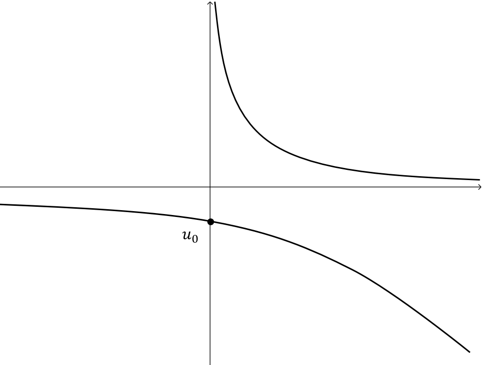
In this figure we have put on the horizontal axis. On the negative side of the vertical axis we have for any fixed , which is a negative quantity for ; whereas on the positive side of the vertical axis we find (or if is convex).
Theorem 2.5.
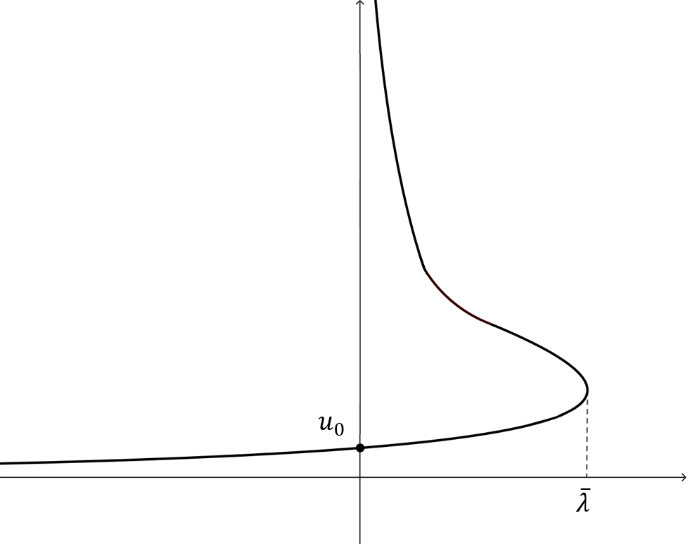
Notice that, up to replacing for , we are also taking into account, indirectly, the case for . We only need to pay attention to the sign of , which is reversed in this case.
In the end, we note that the hypothesis on the boundedness of the coefficients in 2 is only due to the unavailability of any form of the Vázquez strong maximum principle for equations with unbounded coefficients, a rather interesting open problem in itself.
3 Preliminaries
Let be a measurable function satisfying (2). Notice that the condition on the zero order term in (2) means that is proper, i.e. decreasing in , while the hypothesis on the entry implies that is a uniformly elliptic operator. In (2),
are the Pucci’s extremal operators with constants 333We are denoting the ellipticity coefficients by and instead of the usual and in order to avoid any confusions with in the problem 1.3.. See, for example, [9] for their properties. Also, denote , for .
Now we recall the definition of -viscosity solution.
Definition 3.1.
Let . We say that is an -viscosity subsolution respectively, supersolution of in if whenever , and open are such that
for a.e. , then cannot have a local maximum minimum in .
We can think about -viscosity solutions for any , since this restriction makes all test functions continuous and having a second order Taylor expansion [10]. We are going to deal specially with the case .
If and are continuous in , we can use the more usual notion of -viscosity sub and supersolutions – see [11]. Both definitions are equivalent when satisfies 2 with , by proposition 2.9 in [10]; we will be using them interchangeably, in this case, throughout the text.
On the other side, a strong sub or subsolution belongs to and satisfies the inequality at almost every point. As we already mentioned, this notion is intrinsically connected to the -viscosity concept; more precisely we have the following.
Proposition 3.2.
Let satisfy (2) and , . Then, is a strong subsolution supersolution of in if and only if it is an -viscosity subsolution supersolution of this equation.
See theorem 3.1 and proposition 9.1 in [23] for a proof, even with more general conditions on and the exponents . When we refer to solutions of the Dirichlet problem, we will assume that strong solutions belong to , unless otherwise specified. Remember that a solution is always both a sub and supersolution of the equation. It is also well known that the pointwise maximum of subsolutions, or supremum over any set if this supremum is locally bounded, is still a subsolution444See proposition 2 in [21] for a version for -viscosity solutions, , related to quadratic growth..
The next proposition follows from theorem 4 in [33] in the case . For a version with more general exponents and coefficients we refer to proposition 9.4 in [23].
Proposition 3.3.
Stability Let , be operators satisfying (2), , , an -viscosity subsolution supersolution of
Suppose in as and, for each and , if we set
we have as . Then is an -viscosity subsolution supersolution of
The following result, which follows from lemma 2.3 in [33], is a useful tool to deal with quadratic dependence in the gradient. Since we are going to use this result several times in the text, we present a proof in the appendix, for reader’s convenience.
Lemma 3.4.
Exponential change Let and . For set
Then, a.e. in we have , and
| (3.1) | ||||
| (3.2) |
and clearly and .
Moreover, the same inequalities hold in the -viscosity sense if is merely continuous, that is, for example, if is an -viscosity solution of
| (3.3) |
where , then , for , is an -viscosity solution of
| (3.4) |
and analogously for the other inequalities.
We recall some Alexandrov-Bakelman-Pucci type results with unbounded ingredients and quadratic growth, which will be referred to simply by ABP.
Proposition 3.5.
Let be bounded, and for . Then, there exist such that if
then every which is an -viscosity subsolution supersolution of
satisfies, for a constant , the estimate
A consequence of ABP in its quadratic form is the comparison principle for our equations, concerning -viscosity solutions and coercive operators. We give a short proof for reader’s convenience. We make the convention, along the text, that and will always denote a pair of sub and supersolutions, in a sense to be specified.
Lemma 3.6.
Proof.
Set in . By contradiction, assume As on , thus . Set , which is an open nonempty set since . Let and be such that has a minimum at . But then has a minimum at , and by together with the definition of being an -viscosity supersolution, we know that for every , there exists such that, for a.e. , we have
and from the definition of . By (2),
which means that, for , is an -viscosity supersolution of
Then, by ABP with , we have in , which contradicts the definition of . ∎
Remark 3.7.
The same result hods if and , where and are continuous strong sub and supersolutions of (3.7) respectively. Indeed, in the proof above, we only need to note that for some , and consider .
Remark 3.8.
By lemma 3.6 we obtain that for any pair of -viscosity sub and supersolutions of , we have in , for any strong solution of .
The Local Maximum Principle (LMP) is well known, see for example [16], [9], [20], and [25]. Its boundary version (BLMP) is given in theorem 1.3 in [32], without zero order term. We denote with a half ball with a flat portion of the boundary included in .
Proposition 3.9.
Let be a locally bounded -viscosity subsolution of
with , , , for some and , . Then, for each ,
where depends only on and .
The proof, as in [32], is a consequence of LMP. The only difference comes from the need to put the zero order term on the right hand side, applying theorem 3.1(a) of [25], followed by a Moser type approach as in [17]; a detailed proof is given in [29].
We recall two boundary versions of the quantitative strong maximum principle and the weak Harnack inequality, which follow by theorems 1.1. and 1.2 in [32].
Theorem 3.10.
Suppose , . Assume that is an -viscosity supersolution of , in . Then there exist constants depending on , and such that
Theorem 3.11.
Suppose , . Assume that is an -viscosity supersolution of , in . Then there exist constants depending on , and such that
Theorem 3.11 implies, in particular, the strong maximum principle when , i.e. for and an -viscosity solution of , in , where , we have either in or in and if at , then . We will refer to these consequences, along the text, simply by SMP and Hopf.
In [32], theorems 3.10 and 3.11 are proved for , but exactly the same proofs there work for any . Moreover, since the function has a sign, and they are also valid for nonproper operators.
The next two propositions are basic results in the study of first eigenvalues of weighted operators. For a proof with unbounded coefficients, see [28].
Proposition 3.12.
Let , for . Then has a positive weighted eigenvalue corresponding to a positive eigenfunction such that
| (3.11) |
Proposition 3.13.
Let be -viscosity solutions of
| (3.12) |
with for . Suppose one, or , is a strong solution, i.e. belongs to the space . Then for some .
Proposition 3.13 in [28] was stated in terms of -viscosity solutions. However, for equations satisfying (2), the notions of and viscosity solutions are equivalent, by theorem 2.3(iii) in [12] (by using in its proof the ABP with unbounded coefficients from proposition 2.8 in [24]); the addition of the term does not change the proof.
4 Existence results through fixed point theorems
Consider the problem 1.3 without dependence, i.e.
| (4.3) |
under (2). In this section all results hold for functions , and in . About the matrix , it only need to assume that . We set . As for , no sign condition is needed in this section.
We define, under hypothesis (), the operator that takes a function into , the unique -viscosity solution of the problem
| (4.6) |
Claim 4.1.
The operator is completely continuous.
Proof.
Let , in . Then , for all . Set so
We use ABP on the sequence , from where we get . Thus the global estimate from [28] gives us By the compact inclusion of into , there exists and a subsequence such that in . This already shows that takes bounded sets into precompact ones.
We need to see that . This easily follows from the stability proposition 3.3, by defining, for each ,
a.e. , where is the same as with replaced by . Indeed, by (2),
since is increasing, continuous in , with . Since the problem (4.6) has a unique solution, . On the other hand, since this argument can be made for any subsequence of the original , the whole sequence converges to .
∎ Claim 4.1.
The next existence statement is a typical result about existence between sub and supersolutions, and is a version of theorem 2.1 of [14] for fully nonlinear equations. We start with a definition.
Definition 4.2.
An -viscosity subsolution respectively, supersolution of is said to be strict if every -viscosity supersolution subsolution of such that in , also satisfies in .
Set , for any .
Theorem 4.3.
Notice that, under the assumptions of theorem 4.3 and by the global -estimate [28], every solution of (4.3) satisfying in is such that
| (4.7) |
where depends on , , , and, of course, on the uniform bounds on given by and .
Proof.
Consider any , with from (4.7).
Part 1. Existence of a solution in the order interval .
First of all, we construct a modified problem, similar to but a little bit simpler than the one given in [14]. In order to avoid technicalities, consider ; later we indicate the corresponding changes. We set ; for
and also
Consider the problems
| (P) | |||
| () | |||
| () | |||
Notice that, by the construction of and , we have that
| (4.8) |
and the same for . So, are also a pair of strong sub and supersolutions for () and (). Observe also that, since (and the operator still satisfies the conditions in [28]), by (4.7) and the definition of , every solution of () with in is up to the boundary and satisfies
| (4.9) |
so , and is a solution of the original problem (P).
Claim 4.4.
Every -viscosity solution of satisfies in , hence is a solution of , and, by the above, a solution of .
Proof.
Let be an -viscosity solution of (). As in the proof of of lemma 3.6, in order to obtain a contradiction, suppose that is such that As on , it follows that . Consider .
We claim that is an -viscosity supersolution of
| (4.10) |
Indeed, let and such that has a local maximum at in . Then, and has also a local maximum at . By definition of as an -viscosity supersolution of (), for every , there exists an such that
| (4.11) |
since in . Further, from (4.8), a.e. in . Subtracting this from (4.11) and using (2), we obtain a.e. in , since in . Hence, (4.10) is proved.
Next, we move to build a solution for the operator that takes a function into , the unique -viscosity solution of the problem
| (4.14) |
Solutions of () are fixed points of , and belong to the order interval , by claim 4.4. Moreover,
| (4.15) |
for an appropriate . In fact, by observing that
then and if ,
for every . Thus, the -estimates from [28] and ABP, applied to the problem (4.14), give us that and and (4.15) follows.
Notice that takes bounded sets in into precompact ones, by the above and the compact inclusion . Also, if in , then in up to a subsequence; thus we can conclude that is completely continuous if we show that . To prove the latter, similarly to the argument with we set, for ,
where, for each fixed function , the tilde function is the following truncation
Observe that, as it is elementary to check, as . By the estimates for and using that the function is continuous in , we get as and so .
From the complete continuity of and (4.15), the degree is well defined and is equal to one. Indeed, set for all and notice that . Then does not vanish on and
Therefore, has a fixed point , which is a solution of . By claim 4.4, the first existence statement in theorem 4.3 is proved in the case .
If and are in the general case as the maximum and minimum of strong sub and supersolutions, respectively, we define as
and consider . In claim 4.4, choose such that , define and replace by until the end of the proof, observing that implies . The rest of the proof is exactly the same.
Part 2. Degree computation in under strictness of – proof of Theorem 4.3 .
Suppose are strict, and consider the set as in the statement of theorem 4.3. Since there exists a solution of (P) with in , by definition 4.2 we have in and so is a nonempty open set in . Further, from part 1, we see that all fixed points of are in , the degree over is equal to and solutions of (P) and () in coincide, leading to
Denote by the set of fixed points of belonging to the order interval . In claim 4.4 we saw that this set contains the set of fixed points of . The converse is also true since any solution of in the order interval satisfies and (4.9), hence is a solution of , i.e. we have
This set is nonempty by part 1. Also, from that proof, we know that for any sequence with in there exists such that in . Then, if additionally , we obtain that thus is a compact set in .
Now consider, for each , the set .
Claim 4.5.
The family has the finite intersection property, i.e the intersection of any finite number of sets is not empty.
Proof.
Let . Observe that is an -viscosity supersolution of (P), with in . Furthermore, under hypothesis (), such is a minimum of strong solutions of (P), which is exactly what we need to use part 1 of the above proof to obtain the existence of a solution of (P) with in , i.e. and , for every , so . ∎Claim 4.5.
Remark 4.6.
The conclusion of the theorem 4.3 is still true if, instead of , we have some such that , where is a truncation of , i.e. for , for . In this case, and the rest of the proof carries on in the same way.
5 A priori bounds
In this section we prove Theorem 2.1. Now we look at our family of problems 1.3 for , assuming and that the matrix satisfies . Here we consider 2 i.e we suppose that all coefficients of the problem 1.3 are bounded and . With the latter the zero order term in 1.3 is explicit, so we can obtain a clear behavior of the solutions with respect to .
Theorem 5.1.
The proof of theorem 5.1 uses and develops the ideas sketched in [34], adding some improvements in order to remove restrictions on the size of . We start by proving that all supersolutions stay uniformly bounded from below, even when is close to zero.
Proposition 5.2.
Proof.
First observe that both and are -viscosity subsolutions of
Then, using 2, both are also -viscosity subsolutions of
and so is , as the maximum of subsolutions. Moreover, in and on . We make the following exponential change
where is the constant from the definition of Pucci’s operators. From lemma 3.4, we know that is an -viscosity solution of
| (5.3) |
where . Notice that the logarithm above is well defined, since
Now set , where is some fixed supersolution of 1.3, (if there was not such supersolution, we have nothing to prove). Then, by the above, is an -viscosity solution of (). Define
Then since , and in . Also, as a supremum of subsolutions (locally bounded, since it belongs to the interval ), is an -viscosity solution of the first inequality in (). Clearly, on .
Observe that is a coercive operator and the function
with
since . Indeed, from there exists a such that for all i.e. when . If then (notice that ) so take .
Therefore, by the proof of the boundary Lipschitz bound (see theorem 2.3 in [32]),
and so . Observe that the function can be equal to at some interior points.
If there were a sequence of supersolutions of () in with unbounded negative parts, then there would exist a subsequence such that
with for large , since on . Then the respective sequence
i.e. for every , there exists some such that
thus there exists and also
Hence , since on , and .
Finally, define . Then is an -viscosity supersolution of
where is a coercive operator. But this contradicts the following nonlinear version of the SMP. ∎
Lemma 5.3.
Set , for a constant . Let be defined by if , , where . Then, the SMP holds for the operator , i.e. if is a -viscosity solution of
then either in or in .
This lemma can be seen as a form of the Vazquez’s strong maximum principle for our operators, since one over the square root of the primitive of is not integrable at . Actually, it is not difficult to check that we can also have a term in lemma 5.3, for . The proof of lemma 5.3 is given in the appendix.
Note that we apply lemma 5.3 with and .
Before giving the proof of Theorem 5.1 we recall that the class of equations we study is invariant with respect to diffeomorphic changes of the spatial variable. In particular we can assume that the boundary of is a hyperplane in a neighborhood of any given point of . Indeed, straightening of the boundary leads to an equation of the same type, with bounds on the norms of the coefficients depending also on the -norm of .
Proof of Theorem 5.1..
Fix with . From proposition 5.2, there exists a constant such that
| (5.4) |
Suppose then, in order to obtain a contradiction, that solutions are not bounded from above in , by picking out a sequence of -viscosity solutions of 1.3 such that
where is the point of maximum of in , i.e. , .
We claim that, up to changing the blow-up limit point , we can suppose that there is a ball around in which is not identically zero.
To prove the claim, consider , a maximal domain such that in . Obviously there is no need of such argument if or even if in a neighborhood of . Suppose, hence, that is an interior point of , and so for large (considering a half ball in if , after a diffeomorphic change of independent variable which straightens the boundary). Notice that both and satisfy the same equation in , in the -viscosity sense, for each . Now, since there is no zero order terms of this equation in , both and also satisfy this same equation, with on , being, thus, -viscosity sub and supersolutions of , respectively, with strong. We apply lemma 3.6 to obtain that in and, in particular, for large ,
This means that there is blow-up also at the boundary of , in the sense that there exists a sequence with and , as . Next, since is maximal, so , and using on , we have . Therefore, we can take a ball centered at (or a half ball if ) which, by enlarging if necessary, becomes a neighborhood which meets the set ; in another words, such that in . Hence, up to changing and by and , we can suppose that in , or in a half ball if , after straightening the boundary around .
Suppose we are in the more difficult case of a half ball. For simplicity, and up to rescaling, say in , with our equation being defined in .
We take the convention of assuming that the constant may change from line to line and depends on , , , , and . The constant is fixed in (5.4) with its dependence described in the statement of proposition 5.2.
Notice that, from (5.4), for every -viscosity solution of 1.3, the function is a nonnegative -viscosity solution of
where , by 2. Thus, by lemma 3.4, the function
| (5.5) |
is a nonnegative -viscosity supersolution of
| (5.6) |
where and since .
Notice that, in the set , we have and , so
| (5.7) |
Then, using proposition 3.10 applied to (5.6), we obtain positive constants and , depending on and , such that
using (5.7) and that for all . Thus,
| (5.8) |
We claim that this is only possible if , with a constant that does not depend on (and consequently on ), neither . Indeed, if this was not the case, we would obtain a sequence of supersolutions of in such that when and (5.8) holding with replaced by . So, up to a subsequence and renumbering, we can assume that and for all , from where we obtain that
and finally, using ,
| (5.9) |
Taking the limit when we have , since , which contradicts in . More precisely, for the limit in (5.9) we can use, for example, the dominated convergence theorem: for this is obvious; for we use Young’s inequality to estimate
ensuring the desired convergence. In this way we have gotten the claim
Thus, by theorem 3.11 applied to (5.6), we have that there exists other positive constants , depending on and , such that
| (5.10) |
Now we go back to and define
| (5.11) |
which by lemma 3.4 and 2 is an -viscosity solution of
| (5.14) |
where .
As in [14], observe that
| (5.16) |
for any . Now, if we take and then, by Holder’s inequality, the right hand side in (5.16) belongs to and
| (5.17) |
and then
| (5.18) |
6 Proofs of the main theorems
6.1 Some auxiliary results
We start by constructing an auxiliary problem (6.4), for which we can assure that there are no solutions for large , and such that reduces to the problem 1.3. This is a typical but essential (see [3], [14]) argument that allows us to find a second solution via degree theory, by homotopy invariance in .
Fix . Recall that proposition 5.2 gives us an a priori lower uniform bound , depending only on and , such that
| (6.1) |
Consider, thus, the problem
| (6.4) |
for , , satisfying 2, () and (), satisfying , , and being defined as
| (6.5) |
with , , where is the first eigenvalue with weight of the proper operator , associated to the positive eigenfunction , given by proposition 3.12.
Note that every -viscosity solution of is also an -viscosity supersolution of 1.3, since , and so satisfies (6.1). From this and (6.5) we have, for all ,
| (6.6) |
Lemma 6.1.
For each fixed , has no solutions for all and .
Proof.
First observe that every -viscosity solution of , for , is positive in . Indeed, from (6.6), 2 and , we have that is an -viscosity solution of
and this implies that in by ABP. Then in by SMP.
Assume, in order to obtain a contradiction, that has a solution . Again by , (6.6) and 2, we see that is also an -viscosity solution of
and from lemma 3.4,
| (6.9) |
using , where , for and from (6.5). Then (6.9) and (3.11), together with proposition 3.13, yields for . But this contradicts the first line in (6.9), since and in .
∎ Lemma 6.1.
When we are assuming hypothesis () we just say solutions to mean strong solutions of . However, sub and supersolutions of such equations, in general, are not assumed strong (since we are considering the problem in the -viscosity sense), unless specified. In order to avoid possible confusion, we always make explicit the notion of sub/supersolution we are referring to.
The next result is important in degree arguments, bearing in mind the set in theorem 4.3. It will play the role of the strong subsolution in that theorem.
Lemma 6.2.
When has a sign, we will see in the proofs of theorems 2.4 and 2.5 that can be taken as and , respectively, in theorem 4.3 for the problem 1.3, for all .
Proof.
Let be the positive constant from proposition 5.2 such that every -viscosity supersolution of
| (6.12) |
satisfies in . Let be the strong solution of the problem
| (6.15) |
given, for example, by proposition 2.4 in [22]. Then, as the right hand side of (6.15) is positive, by ABP, SMP and Hopf, we have in .
Claim 6.3.
Every -viscosity supersolution of 1.3 satisfies in .
Proof.
Set
Observe that a.e. in and for all . Then,
since and is a strong subsolution of .
Consider the problem , which we define as the problem 1.3 with replaced by , .
Observe that we are in the situation of remark 4.6, since there, which allows us to use theorem 4.3 in order to obtain solutions of .
Let be some fixed strong supersolution of 1.3 (if there were not strong supersolutions of 1.3, the proof is finished). Then, by claim 6.3, we have in . Also, in that proof we observed that , then a.e. , which means that
and so is a strong supersolution of . By theorem 4.3 and remark 4.6, we obtain an -viscosity solution of this problem, with in , which is strong and can be chosen as the minimal solution in the order interval , by hypothesis ().
Remark 6.4.
Notice that a.e. for all , so
| (6.16) |
a.e. in , i.e. is also a strong supersolution of .
Claim 6.5.
For every strong supersolution of 1.3, in .
Proof.
Let be any strong supersolution of 1.3. As in the argument above for , we have that is also a strong supersolution of . Suppose that the conclusion is not verified, i.e. that there exists such that and define
Then is the minimum of strong supersolutions, hence itself is an -viscosity supersolution of and of , by remark 6.4. Following the same lines as in claim 6.3, in . Thus, by theorem 4.3 and remark 4.6, there exists an -viscosity solution of , strong by (), such that in , which gives a contradiction with the minimality of . ∎ Claim 6.5.
Claim 6.6.
is a strong strict subsolution of 1.3.
Proof.
From remark 6.4, and , which implies that actually satisfies (6.16) with equality, from where
| (6.17) |
with on . Thus is a strong subsolution of 1.3. What remains to be proved is that is strict, in order to choose as . Therefore, in the sense of definition 4.2, let be an -viscosity supersolution of 1.3 with in . Then, since is strong, in is an -viscosity supersolution of
in , using 2 and . Hence, for , satisfies
in the -viscosity sense and by SMP, in . If there exists with , Hopf lemma implies that . Then, in . ∎ Claim 6.6.
∎ Lemma 6.2.
6.2 Proof of Theorem 2.3
Suppose, at first, (2), () and ().
We start proving the first statement in theorem 2.3, about existence of solutions for . Set and . Thus, is a pair of strong sub and supersolutions of 1.3, for each , with in . Indeed, using (2), and , we have
| (6.20) |
and similarly for , with , and reversed inequalities. Therefore, theorem 4.3 gives us a solution , for all .
Observe that, since , we can say that for all , by the -estimates [28]. Thus, take a sequence with as . Next, the compact inclusion gives us some such that in , up to a subsequence. Hence we can define, for each ,
| (6.21) |
Then, as . By proposition 3.3, we have that is an -viscosity solution of . From the uniqueness of the solution at , needs to be equal to . Since the sequence of converging to zero is arbitrary, we obtain as .
Now we prove the existence of a continuum from . Fix an and consider another pair of sub and supersolutions and . Analogously to (6.20), we see that are a pair of strong sub and supersolutions for . Notice that they are not a pair for 1.3 with , since they do not have a sign. However, in , which implies that in . Since is the unique -viscosity solution of the problem , then are strict in the sense of definition 4.2. Then, theorem 4.3 gives us, for defined there, that
| (6.22) |
Using again that is the unique -viscosity solution of , we have further that . Then, by the well known degree theory results, see for example theorem 3.3 in [3], there exists a continuum such that both
are unbounded in . This proves item 1.
From now on, we suppose 2.
Let us prove point 2. in theorem 2.3. The continuum is such that its projection on the -axis is either (and we obtain in theorem 2.3) or it is , with . In the second case, since we know that the component is unbounded in , its projection on the axis must be unbounded in .
Under 2, by what we proved in the previous section, for any there is an a priori bound for the solutions of 1.3, for all . Then, by global estimate [28], we have also a a priori bound for these solutions i.e the projection of on is bounded. So, needs to be unbounded in when we approach from the right.
Now, by proposition 5.2, there is a lower bound for the solutions, for every . Therefore, must emanate from plus infinity to the right of , with the positive part of its solutions blowing up to infinity in . Thus, and in 2. are proved.
Now we pass to the multiplicity results in item 3. of theorem 2.3.
Observe that, up to taking a larger in (6.22), by -estimates we can suppose that
| (6.23) |
Claim 6.7.
There exists a such that , for all .
Proof.
Let us prove the existence of a such that, for all , 1.3 has no solution on . Suppose not, i.e. that for all , there exists a such that has a fixed point on . Then for every , there exists and a solution of . By (6.23), and so , for all . Note that
where “touches”, as in [3], has the following meaning.
Definition 6.8.
Let . We say that “touches” if with or with . In any case, at a point .
If “touches” , there exists a such that , and since , then . If by other side “touches” , there exists a ; , and since , then . Anyway,
| (6.24) |
Claim 6.9.
1.3 has two solutions when .
Proof.
By claim 6.7, the existence of a first solution with is already proved. Set . Then, lemma 6.1 implies that has no solutions for and .
Fix a . With replaced by (see (6.5)) we have, by theorem 5.1, an a priori bound for solutions of , for every . Precisely, we get an a priori bound for solutions of , for all , depending on and . This provides, by the -estimates [28], an a priori bound for solutions in , namely
and for some that depends, in addition to the coefficients of the equation, also on and the -norm of . By the homotopy invariance of the degree in and the fact that for the problem has no solution,
where is the operator in which we replace by (of course keeps being completely continuous). But then, by the excision property of the degree,
which provides the second solution that we were looking for.
∎ Claim 6.9.
Claim 6.10.
in and as .
Proof.
Let be a decreasing sequence with , so for . Since , then in , therefore is bounded in by [28]. Hence, exactly as in (6.21), we show by stability that in , where is a solution of . Therefore, .
If, in turn, the respective sequence were uniformly bounded from above, it would be unifomly bounded in using proposition 5.2, so bounded in and the paragraph above would imply that in . Since and is open in , then should belong to for large , for some . But this contradicts the fact that . ∎ Claim 6.10.
Claim 6.11.
In case , the problem has at least one solution.
Proof.
Let be such that and let be a sequence of solutions for . Say for . This provides an a priori bound for , by theorem 5.1, i.e. , which implies that . Again, by compact inclusion and stability, we obtain in , where is a solution of . Surely, for stability we need to consider, this time, and so as .
∎ Claim 6.11.
To finish the proof of theorem 2.3, it remains to show the last statements in item 4. concerning ordering and uniqueness considerations, in which we assume (). Notice that this automatically implies that solutions and are strong, as well as every -viscosity solution of 1.3.
Further, note that () provided existence of minimal and maximal solutions on the order interval in theorem 4.3. Such existence of minimal solution made it possible to find a minimal strong subsolution of 1.3 in lemma 6.2.
Claim 6.12.
, for all .
Proof.
Fix a and consider the strict strong subsolution given by lemma 6.2. Since in particular for every (strong) solution of 1.3, we can choose as the minimal strong solution such that in . This choice implies that
| (6.25) |
Indeed, and, if there would exist such that , by defining , as the minimum of strong supersolutions greater or equal than , so in . Therefore, theorem 4.3 would give us a solution of 1.3 such that , which contradicts the minimality of and implies (6.25).
As far as uniqueness is concerned, from theorem 1(iii) in [33], if the coercive problem for has a strong solution , it is the unique -viscosity solution of 1.3. So, under (), is strong, then unique, in the -viscosity sense, for all . Observe that, in this case, we must have . In another words, the projection of on the -axis contains , as in theorems 1.1 and 1.2 in [2] for the Laplacian.
We finish the proof of 4. with the following claim.
Claim 6.13.
If and is convex in , the solution of , obtained in claim 6.11, is unique.
Proof.
Suppose, in order to obtain a contradiction, that there exist two different solutions and of , both strong by (). Consider . Then, a.e. in ,
using also the convexity of . Hence is a strong supersolution of which is not a solution. Let us see that it is strict. Set , where is an -viscosity subsolution of with in . Thus, is an -viscosity solution of
and so, by lemma 3.4, the function , where , is a nonnegative -viscosity solution of in , with . Then SMP gives us that in . Now, Hopf and on imply in the boundary points where , and so on . Consequently, in and is a strict strong supersolution of .
Consider also the strict strong subsolution of given by proposition 6.2 and look to the set . By the -estimates in [28],
| (6.26) |
for some that depends on the -norm of . Then, by theorem 4.3, we obtain such that , where .
We claim that there exists such that
| (6.27) |
As in the proof of claim 6.7, we will verify that there exists some such that there is no fixed points of on the boundary of , for all in the preceding interval. Indeed, if this were not the case, there would exist a sequence with the respective solutions of belonging to . Say for . Then, since in , by (6.26) we must have for , which means that for each such ,
| (6.28) |
By (6.26) and the compact inclusion , in for some , up to a subsequence. This is an -viscosity solution of by the stability proposition 3.3; and in by taking the limit as in the corresponding inequalities for . Thus in , since and are strict. Passing to the limit into (6.28), we obtain that “touches” or , which contradicts the definition of .
Hence, obtaining (6.27) is just a question of applying homotopy invariance in in the interval . Next, with (6.27) at hand, we repeat exactly the same argument done in claim 6.9 to obtain the existence of a second solution of 1.3, for all . But this, finally, contradicts the definition of . ∎ Claim 6.13.
6.3 Proof of Theorem 2.4
Claim 6.14.
is a strict strong supersolution of 1.3, for all .
Proof.
Since in , is a strong supersolution of 1.3 which is not a solution. To see that it is strict, we take an -viscosity subsolution of 1.3 such that in , and set . Then, since is strong, is an -viscosity supersolution of
and so in in the -viscosity sense, for and , , using lemma 3.4. Using SMP and the fact that is not a solution of 1.3, we have in . Since on , at points belonging to such that we are done. If in turn is such that , then by Hopf. Thus and so in . ∎ Claim 6.14.
We now prove that for all , 1.3 has at least two solutions, and , with and .
Fix a . From lemma 6.2 and step 1, we get a pair of strong strict sub and supersolutions, and , which implies, by theorem 4.3, the existence of a first solution , where in for some .
Remark 6.15.
Fix a and set . As in the proof of claim 6.9, we observe that, by lemma 6.1, has no solutions for . Moreover, for replaced by , theorem 5.1 gives us an a priori bound for solutions of for every , which depends on . This provides, by the global estimates [28], an a priori bound for solutions in , i.e. for every solution of , for all , where also depends on . By the homotopy invariance of the degree,
Therefore, by the excision property of the degree
and the existence of a second solution is derived.
Since the argument above can be done for any , we obtain the existence of at least two solutions for every positive . Exactly the same reasoning from claims 6.12 and 6.10 applies to check that in and to get their behavior when , respectively, since is the same from theorem 2.3. Of course, here .
Claim 6.16.
For , we have in .
Proof.
For fixed note that since . Then, is a strong supersolution of which is not a solution and, in particular, .
We first infer that in . In fact, similarly to the argument in the proof of claim 6.12, recall that , given by lemma 6.2, is such that for every strong supersolution of , and in particular . Remember also that is the minimal strong solution such that in . Now, if there was a such that , by defining , as the minimum of strong supersolutions of not less than , we have in . Thus, theorem 4.3 provides a solution of such that in , which contradicts the minimality of .
Proceeding as usual, becomes a nonnegative strong supersolution of in , then SMP gives us that in , since ; Hopf and on imply that , so on . ∎ Claim 6.16.
Remark 6.17.
Notice that in , for every nonpositive -viscosity subsolution of 1.3 in . Indeed, since in , is also an -viscosity subsolution of . By remark 3.8, , since is strong. Now, by claim 6.14 and definition of strict supersolution, we get in .
In particular, is never a solution of 1.3, for any recall that .
Claim 6.18.
Proof.
Suppose, in order to obtain a contradiction, that there exist two different nonpositive solutions and , strong by (). By remark 6.17 we know that and in . We can assume that they are ordered, in the sense that . Indeed, observe that , then by theorem 4.3 we obtain a solution of 1.3 satisfying in . Thus, if the solutions and do not satisfy , then there is a point with , which implies that and so ; in this case we just replace by respectively.
Since (from and ), the quantity is well defined and finite. Further, , since , so this infimum is attained. Then, by setting , we have that satisfies and it is a strong subsolution of
since is convex in and is convex in . Now, by remark 6.17 we have in , i.e. in . Then, there exists a little bit smaller such that in (see the argument in [28], for example, by taking a compact set with small measure containing the boundary). Therefore, this last contradicts the definition of as a minimum. ∎ Claim 6.18.
6.4 Proof of Theorem 2.5
Suppose for the time being just with in and 2.
Claim 6.19.
We have , for every nonnegative -viscosity supersolution of 1.3, for all .
Proof.
Notice that in implies that is an -viscosity supersolution of . Since is strong, by remark 3.8, in . But is not a solution of 1.3 for since , which means that .
Set in . Then, using , we see that is a nonnegative -viscosity supersolution of
with , as usual. By SMP, in . If on it is done; if by other side there exists with , we apply Hopf lemma to obtain . Therefore, in . ∎ Claim 6.19.
Claim 6.20.
1.3 has no nonnegative -viscosity solutions for large.
Proof.
Let , where is the principal weighted eigenvalue of
associated to , from proposition 3.12, i.e.
| (6.32) |
Suppose, in order to obtain a contradiction, that there exists a nonnegative -viscosity solution of 1.3 and set in . By claim 6.19, in .
Since is strong, we can use it as a test function into the definition of -viscosity supersolution of , together with 2 and , to obtain that
since , and so satisfies
| (6.35) |
in the -viscosity sense. As the proof of lemma 6.1, applying proposition 3.13 to (6.35) and (6.32), we get for . But this contradicts the first line in (6.35), since in . ∎ Claim 6.20.
Define
which is finite, by claim 6.20. Of course it is well defined and nonnegative, since . Also, by the definition of , 1.3 has no nonnegative solutions for .
It is a subtle but important detail that is a positive number. In fact, by the existence of the continuum, theorem 2.3, we know that, for small, there exists a solution of such that , since . But why can we infer that for small positive? This is the subject of the next claim.
Consider hypothesis () from now. Then, -viscosity solutions of 1.3 are strong.
Claim 6.21.
.
Proof.
Let , where is such that there exists a nontrivial solution of 1.3 in this interval, as indicated above. Suppose , where is a lower bound for the solutions of 1.3 such that , for all . We are supposing here , otherwise every solution of 1.3 would be nonnegative for .
Suppose firstly that . In this case every nontrivial solution of 1.3 satisfies
Then in by ABP, for all .
Remark 6.22.
Another way to prove claim 6.4 is by considerations on first eigenvalues, which provide an estimate on the smallness of .
Set , with an -viscosity solution of 1.3 for , where is the constant from ABP for . Of course, negativity of implies that in . So, in order to obtain a contradiction, suppose that .
Notice that is an -viscosity solution of in , with on . Thus, as in the proof of proposition 3.4 in [33], we use ABP to obtain that which, by the choice of , is a contradiction.
Claim 6.23.
For each , 1.3 has a well ordered strict pair of strong sub and supersolutions, namely in .
Proof.
Let . As the strict subsolution we just consider again, which is strong. Note that is strict, since for any supersolution such that in , we have , by repeating the final paragraph in the proof of claim 6.19.
Note that, from the definition of , there exists and a nonnegative solution of . By claim 6.19, in . On the other hand, since
we have and so is a supersolution of 1.3 which is not a solution. In addition, is strict because if is an -viscosity subsolution of 1.3 with in , by defining and arguing as usual when we have a strong supersolution, becomes an -viscosity supersolution of
with . Thus, , for , is a -viscosity supersolution of in by lemma 3.4. Then, SMP gives us in and so in , by applying Hopf at the boundary bounds where . Consequently, in .
Therefore, we can define for , for all .
∎ Claim 6.23.
Next, we work a little bit more to construct the second solution that also satisfies but is not on (as in [14]). For this, fix a and consider the open subset of defined by
which contains the set from theorem 4.3, since .
Analogously to the proof of claim 6.9, we obtain an a priori -bound for the solutions of which depends on but not on , related to for some small . This provides a which bounds the norm of the solutions, by the -estimates. Then, by the homotopy invariance of the degree in and the fact that there is no solution for , we have . Therefore, by excision, , which provides a second solution , i.e. a solution that satisfies, by construction, in , for , for every . In particular, this second solution is also nonnegative and nontrivial for all .
Under (), theorem 4.3 (ii) allows us to choose as the minimal strong solution between and . As the proof of claim 6.12, this implies (6.25). Indeed, and, if existed such that , by defining , as the minimum of strong supersolutions greater or equal than , we have in . Also, in . By theorem 4.3 there exists a solution of 1.3 such that , which contradicts the minimality of , since is a solution which belongs to the order interval .
Therefore, defining in , we see that is a nonnegative strong solution of in . Thus, since , SMP yields in and Hopf concludes that in , i.e.
in , for all .
Claim 6.24.
For , we have in .
Proof.
The proof is similar to the proof of claim 6.23, but a little bit simpler since both and are strong. However, we repeat it here to avoid confusions about notation. For fixed , we have since
Then, is a supersolution of that is not a solution. In particular, .
Next in . In fact, if there was a point such that , by defining , the minimum of strong supersolutions of larger than , we have that in . By theorem 4.3, there exists a solution of such that , which contradicts the minimality of , since is a solution that belongs to the order interval .
Hence is a strong supersolution of in , for . Then SMP yields in , since . Hopf and on give us , so in . ∎ Claim 6.16.
The existence proof of at least one solution for follows exactly the same lines as the proof of claim 6.11 since, in there, we only used the fact that there exists one sequence of solutions corresponding to a maximizing sequence of ’s converging to the supremum . Furthermore, uniqueness is true if is convex in , by following the proof of claim 6.13. Finally, the behavior of the solutions is the same as in claim 6.10 and this finishes the proof of theorem 2.5.
Remark 6.25.
Particular cases of theorems 2.4 and 2.5 are and , respectively. Indeed, if and holds, then is a strong supersolution of
with on . Then SPM gives us in and so . Furthermore, by Hopf, in .
On the other hand, if and holds, then is a strong subsolution of
and so , for , is a strong subsolution of in by lemma 3.4, with on . Again by SMP we get in then in by Hopf and so does with , from where .
7 Appendix
7.1 Proof of Lemma 5.3
For maximal generality we show that the result is valid for the most general notion of -viscosity solutions (see [11], [20]), which can be discontinuous functions. We can suppose , just replacing by its lower semi-continuous envelope , defined as . In this case, we say that is a -viscosity supersolution if is.
By contradiction, let be a nonnegative -viscosity supersolution of
with both and nonempty sets. Notice that is open, since . As in the usual proof of SMP (see, for instance, [4]), choose such that and consider the ball such that .
Observe that is a strictly increasing function on the interval , .
Fix a , so and in . Note that, up to diminishing , we can suppose also that in . Indeed, since there exists a ball such that in this ball; so by taking with for a point , now just replace by .
Consider the annulus centered in and set . We need to find a good barrier in for our nonlinear problem. This is accomplished in the following claim.
Claim 7.1.
There exists a nonnegative classical subsolution of
which is radially decreasing in , convex and such that on .
Proof.
We start choosing a large such that
| (7.1) |
where , for .
Let be such that and set
| (7.2) |
Remark 7.2.
See, for instance, lemma 2.2 in [33] Suppose that is a radial function, say , defined in a ball centered on . Then
With this choice of , of course on and on . Notice that with , thus and so
for every , where is the interior unit normal to the ball . Further, , and by remark 7.2 we have, in ,
by the choice of in (7.1). Now we claim that
| (7.3) |
and this will finish the proof of the claim 7.1. For this is obvious. Note that, for , (7.3) is equivalent to
| (7.4) |
But the left hand side of (7.4) is less or equal than
by using and definitions of , , where for .
∎ Claim 7.1.
By construction, on .
Claim 7.3.
in .
Proof.
Suppose not, i.e. that the open set is not empty.
Notice that since is decreasing in and on , then both in , and we can use the monotonicity of in to obtain
in the -viscosity sense, and so the comparison principle (for example proposition 3.3 in [20]), gives us that in , which contradicts the definition of .
∎ Claim 7.3.
To finish the proof of lemma 5.3, if , we can just use the fact that has a minimum at the interior point , so by claim 7.3 we have , a contradiction.
Assume is only in . Let . Observe that is a function in with in and, since in with , then touches from below at the interior point . Thus, by definition of being a -viscosity supersolution on , we get
7.2 Proof of Lemma 3.4
The proof follows the original idea of [33] for viscosity solutions, with the slight improvements that can be found in theorem 6.9 in [20].
Proof.
Inequalities (3.1) and (3.2) follow by a simple computation, by using the fact that , where , for all . Suppose, then, that is an -viscosity solution of (3.3).
Let such that attains a local maximum at , namely and , and let . Take some with and set .
Define , i.e. then, since has a maximum at , by using the definition of being an -viscosity subsolution of (3.3) and also (3.1) for the pair , we get
where and is some subset with positive measure.
Let . Notice that, since and for , there exists such that in . Thus and
i.e. we have shown that is an -viscosity subsolution of
for any . The desired conclusion follows by letting , since for any , where , by proposition 3.3. The proof of the remaining inequalities in the -viscosity sense are similar. ∎
Corollary 7.4.
Let , , for , , and a locally bounded -viscosity solution of
then is twice superdifferentiable subdifferentiable a.e. in .
Proof.
As a matter of fact, corollary 7.4 is true for as in [10], since lemma 3.4 also holds in this case. Moreover, it follows from the argument in [10], that locally bounded -viscosity solutions of , with satisfying the structure condition in 2 , are twice differentiable a.e. and satisfy the equation at almost all points.
References
- [1] Abdellaoui, B., Dall’Aglio, A., Peral, I. Some remarks on elliptic problems with critical growth in the gradient. J. Differential Equations 222, (2006), 21–62.
- [2] Arcoya, D.; Coster, C.De; Jeanjean, L.; Tanaka, K. Continuum of solutions for an elliptic problem with critical growth in the gradient. J. Funct. Anal. 268 (8) (2015), 2298-2335.
- [3] Bandle, C.; Reichel, W. Solutions of quasilinear second-order elliptic boundary value problems via degree theory. In: Chipot, M.; Quittner, P. (Eds.) Handbook of Differential Equations, Stationary Partial Differential Equations, vol.1. Elsevier, NorthHolland, Amsterdam (2004), 1–70.
- [4] Bardi, M.; Da Lio, F. On the strong maximum principle for fully nonlinear degenerate elliptic equations. Arch. Math. (Basel), 73 (1999), 276-285.
- [5] G. Barles, A. Blanc, C. Georgelin, M. Kobylanski, Remarks on the maximum principle for nonlinear elliptic PDEs with quadratic growth conditions. Ann. Sc. Norm. Sup. Pisa 28(3) (1999), 381–404.
- [6] G. Barles, F. Murat, Uniqueness and the maximum principle for quasilinear elliptic equations with quadratic growth conditions. Arch. Rat. Mech. Anal. 133(1) (1995), 77–101.
- [7] Boccardo, L.; Murat, F.; Puel, J.P. Résultats d’existence pour certains problèmes elliptiques quasilinéaires. Annali della Scuola Normale Superiore di Pisa-Classe di Scienze 11, (1984), 213-235.
- [8] Boccardo, L.; Murat, F.; Puel, J.P. Existence des solutions faibles des équations elliptiques quasi-lineaires à croissance quadratique. In: H. Brézis, J.L. Lions (Eds.), Nonlinear P.D.E. and Their Applications, Collège de France Seminar, vol. IV, Research Notes in Mathematics, vol. 84, , Pitman, London (1983), 19–73 .
- [9] Caffarelli, L. A.; Cabré, Xavier. Fully nonlinear elliptic equations. American Mathematical Society Colloquium Publications, 43. American Mathematical Society, Providence, RI, vi-104 pp. (1995).
- [10] Caffarelli, L.; Crandall, M.G.; Kocan, M.; Świech, A. On viscosity solutions of fully nonlinear equations with measurable ingredients. Comm. Pure Appl. Math. 49 (1996), 365–397.
- [11] Crandall, M.G.; Ishii, H.; Lions, P.L. User’s guide to viscosity solutions of second order partial differential equations. Bull. Amer. Math. Soc. (N.S.) 27 (1992), 1–67.
- [12] Crandall, M. G.; Kocan, M.; Soravia, P.; Świech, A. On the equivalence of various weak notions of solutions of elliptic PDEs with measurable ingredients. Progress in elliptic and parabolic partial differential equations, Capri (1994), 136–162.
- [13] De Coster, C.; Fernández, A. J. Existence and multiplicity for elliptic p-Laplacian problems with critical growth in the gradient. Preprint, arXiv:1801.04155.
- [14] De Coster, C.; Jeanjean, L. Multiplicity results in the non-coercive case for an elliptic problem with critical growth in the gradient. J. Differential Equations, 262, (2017), 5231-5270.
- [15] V. Ferone, F. Murat, Nonlinear problems having natural growth in the gradient: an existence result when the source terms are small. Nonl. Anal. 42(7) (2000), 1309–1326.
- [16] Gilbarg, D.; Trudinger, N.S. Elliptic partial differential equations of second order Springer, 2nd ed (2000).
- [17] Han, Q.; Lin, F. Elliptic partial differential equations. Courant Lecture Notes Math., v. 1, AMS, Providence, RI (1997).
- [18] Jeanjean, L.; Sirakov, B. Existence and multiplicity for elliptic problems with quadratic growth in the gradient. Comm. Part. Diff. Eq. 38, (2013), 244-264.
- [19] Kazdan, J.L.; Kramer, R.J. Invariant criteria for existence of solutions to second-order quasi-linear elliptic equations. Comm. Pure Appl. Math., 31 (5) (1978), 619-645.
- [20] Koike, S. A Beginner’s guide to the theory of viscosity solutions. 2nd ed (2010).
- [21] Koike, S. Perron’s method -revisited. Surikaisekikenkyusho Kokyuroku, 1428 (2005), 1-8.
- [22] Koike, S.; Świech, A. Existence of strong solutions of Pucci extremal equations with superlinear growth in . J. Fixed Point Theory Appl. 5 (2009), no. 2, 291-304.
- [23] Koike, S.; Świech, A. Weak Harnack inequality for fully nonlinear uniformly elliptic PDE with unbounded ingredients. J. Math. Soc. Japan. 61 (2009), no. 3, 723-755.
- [24] Koike, S.; Świech, A. Maximum principle for fully nonlinear equations via the iterated comparison function method. Math. Ann. 339 (2007), no. 2, 461-484.
- [25] Koike, S.; Świech, A. Local maximum principle for Lp-viscosity solutions of fully nonlinear PDEs with unbounded ingredients. Communications in Pure and Applied Analysis, 11(5), (2012), 1897-1910.
- [26] Milakis, E.; Silvestre, L. Regularity for fully nonlinear elliptic equations with Neumann boundary data Comm. Partial Differential Equations, 31 (8) (2006), 1227–1252.
- [27] Munkres, J. R. Topology. Prentice Hall, Upper Saddle River, NJ 07458, 2nd ed. 2000.
- [28] Nornberg, G. S. regularity for fully nonlinear equations with superlinear growth in the gradient. arxiv:1802.01643
- [29] Nornberg, G. S. Methods of the regularity theory in the study of partial differential equations with natural growth in the gradient. PhD thesis, PUC-Rio (2018).
- [30] Pimentel, E. A.; Teixeira, E. V. Sharp Hessian integrability estimates for nonlinear elliptic equations: an asymptotic approach. J. Math. Pures Appl. (9) 106 (2016), no. 4, 744–767.
- [31] Silvestre, L.; Sirakov, B. Boundary regularity for viscosity solutions of fully nonlinear elliptic equations Comunications in Partial Differential Equations v. 39, Issue 9 (2014), 1-24.
- [32] Sirakov, B. Boundary Harnack estimates and quantitative strong maximum principles for uniformly elliptic PDE. International Mathematics Research Notices, Vol. 2017, No. 00, (2017), 1–26.
- [33] Sirakov, B. Solvability of uniformly elliptic fully nonlinear PDE. Archive for Rational Mechanics and Analysis v. 195, Issue 2, 579-607 (2010).
- [34] Sirakov, B. Uniform bounds via regularity estimates for elliptic PDE with critical growth in the gradient. arXiv:1509.04495
- [35] Souplet, P. A priori estimates and bifurcation of solutions for an elliptic equation with semidefinite critical growth in the gradient. Nonlinear Anal. 121 (2015), 412–423.
- [36] Winter, N. and estimates at the boundary for solutions of fully nonlinear, uniformly elliptic equations. Z. Anal. Anwend. 28 (2009), 129-164.