ComPAS: Community Preserving Sampling
for Streaming Graphs

Abstract.

In the era of big data, graph sampling is indispensable in many settings. Existing sampling methods are mostly designed for static graphs, and aim to preserve basic structural properties of the original graph (such as degree distribution, clustering coefficient etc.) in the sample. We argue that for any sampling method it is impossible to produce an universal representative sample which can preserve all the properties of the original graph; rather sampling should be application specific (such as preserving hubs - needed for information diffusion). Here we consider community detection as an application scenario. We propose ComPAS, a novel sampling strategy that unlike previous methods, is not only designed for streaming graphs (which is a more realistic representation of a real-world scenario) but also preserves the community structure of the original graph in the sample. Empirical results on both synthetic and different real-world graphs show that ComPAS is the best to preserve the underlying community structure with average performance reaching 73.2% of the most informed algorithm for static graphs.

1. Introduction

One of the fundamental techniques to analyze very large-scale graphs is through sampling Leskovec and Faloutsos (2006), especially where the analysis on the entire graph is intractable (and often impractical). A good sampling method should usually target a specific application and essentially preserve a set of (not all) properties of the original graph geared toward the application. For instance, a sampling method designed for information diffusion should preserve the hubs (high-degree nodes) in the sample; whereas, a sampling scheme for outbreak detection (such as disease outbreak) should preserve the nodes with high local clustering coefficient. Sampling has been studied extensively in the context of static graphs Leskovec and Faloutsos (2006); Gjoka et al. (2010); Maiya and Berger-Wolf (2010); Rasti et al. (2009); Ribeiro and Towsley (2010); however, there has been very limited work on sampling from streaming graphs Henzinger et al. (1998) where nodes/edges arrive in discrete time intervals and only a part of the entire graph is available for analysis at any point of time Aggarwal et al. (2011); Ahmed et al. (2014); Lim and Kang (2015); Stefani et al. (2017).

Existing graph sampling methods are mostly designed for preserving simple structural properties (such as degree distribution, clustering coefficient etc.) of the original graph in the sample - only few works attempted to preserve complex properties like community Tong et al. (2016); Maiya and Berger-Wolf (2010) - which may be useful for designing a wide range of applications. For instance, in marketing, surveys often seek to construct samples from different communities to capture the diversity of the population (also known as cluster sampling) Kolascyk (2013). In this paper, we propose a novel sampling algorithm that preserves the original community structure of streaming graphs. Our work sharply contrasts the recently proposed Green Algorithm (GA) Tong et al. (2016) which, is explicitly designed to generate a sample that preserves the community structure for static graphs.

Our contributions: In this paper, we propose ComPAS, a novel sampling algorithm on streaming graph (most realistic graph representation Aggarwal et al. (2011); Ahmed et al. (2014)) that is capable of preserving the community structure of the original graph.

ComPAS is designed based on a novel hypothesis that graph sampling and community detection can be interwoven together to produce a more representative sample. In particular, our contributions in this paper are the following:

• To the best of our knowledge ComPAS is the first community-preserving sampling method for streaming graphs. Along with the sample nodes, ComPAS also outputs the community structure of the sample that closely corresponds to the community structure of the original graph.

• In absence of any other community preserving sampling algorithm for streaming graphs, we resort to comparing ComPAS  with GA Tong et al. (2016) which was designed to preserve the community structure while sampling from static graphs. Note that GA, unlike ComPAS, has the information of the full graph while sampling and building the community structure. Empirical evidences on synthetic and real-world graphs demonstrate that the sample generated by ComPAS correctly preserves the community structure with average performance reaching as high as 73.2% of GA. Further, we also compare ComPAS with well-known node/edge preserving sampling methods available for streaming graphs to show that these do not automatically preserve the community structure thus necessitating the design of ComPAS .

• We do a detailed micro-analysis to comprehend the reasons behind superior performance of ComPAS. We also show additional benefits of ComPAS through an application – selection of (limited) training set for online learning. We obtain a performance that is within 90.5% of the most informed algorithm GA available for static graphs.

2. Related work

Population sampling has been studied for long in social sciences Frank (1977),Frank (1980), such as snowball sampling Goodman (1961), respondent-driven sampling Heckathorn (1997), Gile and Handcock (2010) etc. and most of the relevant works in this space deal with estimating global properties of the population (see a survey in Kolascyk (2013)).

Sampling from static graphs: Availability of large-scale graph data has generated renewed interest in the sampling problem  Leskovec and Faloutsos (2006); Gjoka et al. (2010); Rasti et al. (2009); Ribeiro and Towsley (2010); Ahmed et al. (2010). Following in this series are works like Maiya and Berger-Wolf (2010) and Maiya and Berger-Wolf (2011). A severe limitation of these approaches is that they assume that the entire graph is present in advance (i.e., the snapshot is static) for the algorithm to produce the desired output.

Sampling from streaming graphs: With increasing interest in mining and analysis of large social graphs (which are mostly dynamic in nature), there is a recent shift in focus toward sampling from streaming graphs. A streaming graph corresponds to a stream of incoming edges (see Figure 1). Aggarwal et al. (2011) proposed a streaming edge sampling (SE) algorithm for outlier detection. Ahmed et al. (2014) proposed streaming node sampling (SN), streaming BFS (Breadth First Search, SBFS) and Partially Induced Edge Sampling (PIES) algorithms. SN and SE maintain a reservoir of nodes and edges respectively and insert or remove them based on a pre-defined hash function. While SBFS essentially implements simple breadth-first search on a sliding window of fixed number of edges in the stream, PIES leverages a partial induction of nodes and combines edge-based node sampling with the graph induction in a single pass. Other recent works include Lim and Kang (2015); Stefani et al. (2017).

The most informative baseline: The Green Algorithm (GA) Tong et al. (2016) is capable of generating community structure preserving samples for static graph; however, the explicit community structure is not produced as an output of the algorithm. This constitutes, for us, the most informative baseline since it has to have the full original network at its disposal to decide whether to include an edge or node in the sample it constructs. Typically the set of nodes with high clustering coefficients as well as high degree are sampled in. However, for a streaming graph setting, this exercise becomes difficult as one needs to determine the importance of a node based only on its limited arrival history. To this aim we incorporate a simple technique which allows ComPAS to correctly identify the high fidelity (high degree and clustering coefficient) nodes and, thereby, improve the quality of the sample. Moreover, we intend to create samples in such a way that the nodes thus sampled are largely connected among themselves. This may be specially important for problems where edge characteristics are necessary like link prediction De et al. (2013), epidemic flow modeling Li et al. (2013), signed network friend/foe classification Leskovec et al. (2010).

3. Problem definition

We consider a graph stream $S$ represented by a set of edges $e_{1}$, $e_{2}$, $\cdots$ with each edge $e_{i}$ arriving at $i^{th}$ (discrete) time step. A graph $G$ at time $t$ is the aggregate of all the edges arriving till time $t$. $V$ represents the set of unique nodes present in $G$. The community structure of $G$ is represented by $C$. We consider $G$ to be both unweighted and undirected.

Definition 1.

Given a streaming graph $G$ of size $V$, our objective is to obtain a sample graph $G_{s}$ of size $n$ such that $C$, the underlying community structure of $G$ is highly preserved in $G_{s}$ $($i.e., $C\sim C_{s}$ where $C_{s}$ is the community structure of $G_{s})$ given the constrain that any algorithm at any discrete time step can only utilize the information of last arrived $\mathcal{H}$ ($<<$ $V$, $n$) nodes (which is maintained in a buffer).

Data: $S$: Graph stream, $n$: Sample size, $\alpha$: Initial fraction of nodes inserted, $n_{d}$: size of the buffer, $Algo$: a community detection algorithm

Result: Sampled subgraph $G_{s}(V_{s},E_{s})$, $C_{s}$

1 Initialize $G_{s}$: $V_{s}=\phi$, $E_{s}=\phi$

2 Create an empty buffer $\mathcal{H}$ of size $n_{d}$

3 Initialize buffer $\mathcal{H}$: $\mathcal{H}_{c}=\phi$, $\mathcal{H}_{p}=\phi$

4 $flag=1$, $t=0$

5 for $e_{t}$ in the graph stream $S$ do

6       $e_{t}=\{u,v\}$

7       if $\frac{|V_{s}|}{n}<\alpha\wedge e_{t}\notin E_{s}$ then

8             $V_{s}=V_{s}\cup u\cup v$

9             $E_{s}=E_{s}\cup e_{t}$

10             Continue;

11      else if flag==1 then

12             Run $Algo$ on $G_{s}$ and detect community structure $C_{s}$

13             $flag$=0

14            

15      else if $u,v\in V_{s}$ then

16             $V_{s},E_{s},C_{s}=BothinSample(u,v,e_{t},V_{s},E_{s},C_{s})$

17            

18      else if $u,v\notin V_{s}\wedge u,v\in\mathcal{H}$ then

19             $\mathcal{H}=NodeinBuffer(u,\mathcal{H})$

20             $\mathcal{H}=NodeinBuffer(v,\mathcal{H})$

21      else if $u\in V_{s}\wedge v\notin V_{s}\wedge v\in\mathcal{H}$ then

22             $\mathcal{H}=NodeinBuffer(v,\mathcal{H})$

23            

24      else if $u\in V_{s}\wedge v\notin V_{s}\wedge v\notin\mathcal{H}$ then

25             $V_{s},E_{s},C_{s},\mathcal{H}=NodeisNew(v,u,V_{s},E_{s},\mathcal{H},C_{s})$

26      else if $u\notin V_{s}\wedge u\in\mathcal{H}\wedge v\notin V_{s}\wedge v\notin\mathcal{H}$ then

27             $\mathcal{H}_{c}(u)=\mathcal{H}_{c}(u)+1$

28             $V_{s},E_{s},C_{s},\mathcal{H}=NodeisNew(v,u,V_{s},E_{s},\mathcal{H},C_{s})$

29      else if $u,v\notin V_{s}\wedge u,v\notin\mathcal{H}$ then

30             $V_{s},E_{s},C_{s},\mathcal{H}=NodeisNew(u,v,V_{s},E_{s},\mathcal{H},C_{s})$

31             $V_{s},E_{s},C_{s},\mathcal{H}=NodeisNew(v,u,V_{s},E_{s},\mathcal{H},C_{s})$

32      $t=t+1$

33

return $G_{s}$, $C_{s}$

Algorithm 1 ComPAS: A Community Preserving Sampling Algorithm for Streaming Graph

4. Proposed algorithm: ComPAS

We propose ComPAS, a Community Preserving sampling Algorithm for Streaming graphs. ComPAS aims at sampling a streaming graph in such a way that its underlying community structure is preserved in the sample (Algorithm 1 and Figure 1 respectively present a pseudo-code and a toy example). The algorithm attempts to identify the high fidelity nodes (nodes with high degree and high clustering coefficient) and suitably determine the communities to which they belong.
Description of the algorithm: To start with, ComPAS keeps adding streaming edges (nodes) into the sample $G_{s}$ as long as a certain number of nodes ($\alpha\cdot n$, $\alpha\leavevmode\nobreak\ <\leavevmode\nobreak\ 1$) are inserted (lines 1-1). This constitutes the warm-up knowledge for the structure. Once the threshold is reached, a pre-selected community detection algorithm $Algo$ is run on $G_{s}$ to obtain the initial community structure (line 1).

Subsequent dynamics: Henceforth, once an edge $e_{t}$ is picked up from the stream, ComPAS inserts $e_{t}$ into a buffer $\mathcal{H}$ (size $n_{d}$) which consists of the two variables – $\mathcal{H}_{c}$ and $\mathcal{H}_{p}$. $\mathcal{H}_{c}$ counts the number of times a node is encountered till that time, and $\mathcal{H}_{p}$ keeps track of the current parent of a node (i.e., the node with which it arrived last). This presents a crude estimation of the importance of the node, since a recurrently occurring node is probably more important compared to a node occurring only intermittently. The idea is inspired by the reservoir sampling technique introduced in Ahmed et al. (2014). Once the buffer $\mathcal{H}$ is full, the insertion activity triggers some chain reactions which are different at the two specific phases (a). when the size of $G_{s}$ is between $\alpha\cdot n$ and $n$ - any incoming new node triggers the entry of a node($x$) and corresponding edge ($\mathcal{P}(x)$, $x$) from buffer to $G_{s}$ and (b). when $G_{s}$ has already reached $n$ - at that point a node has to be removed from $G_{s}$ to insert the incoming node ($x$) from buffer. We eliminate the node with least degree and clustering coefficient thus ensuring progressive inclusion of high-fidelity node.

Genesis of the six modules of ComPAS: Considering differently, for an incoming streaming edge $e_{t}\leavevmode\nobreak\ =\leavevmode\nobreak\ \{u,v\}$, each endpoint ($u,v$) could be (i) a new node, (ii) present in the buffer or (iii) present in the partially constructed sample graph $G_{s}$. Depending on the current position of $u$ and $v$, one of the six conditions is encountered which are consequently handled by the six submodules - (1) both endpoints are present in the sample, (2) both are in buffer, (3) one is in sample while the other is in buffer, (4) one is in sample while the other is new, (5) one is in buffer while the other is new and (6) both are new. We elaborate on the submodules next.

(i) Both $u$ and $v$ are present in the Graph $G_{s}$: When both $u,v$ are in $V_{s}$, $BothinSample()$ (see Function 2) is called from line 15 of Algorithm 1. The aim of this module is to place the edge in such a way that the modularity of the evolving sample graph ($G_{s}$) improves. Vis-a-vis the existing community structure, the edge $e_{t}$ can be (a). an intra-community edge (totally inside a single community) or (b). an inter-community edge (connecting two communities $C(u)$ and $C(v)$).

In case of an intra-community edge (edge $\{b,d\}$ in Figure 1), addition of $e_{t}$ increases modularity of the community according to Proposition 1. Moreover, we also know from Proposition 2 that splitting of current community on addition of a new intra-community edge does not increase modularity Ye et al. (2008). Therefore we leave $C_{s}$ in its current form without any modification.

Proposition 1.

Addition of an edge to a community $c\in C$, increases its modularity if $D_{c}\leq M-1$ $($where $M=|E|$ and $D_{c}$ is total degree of all the nodes $c$ ).

Proposition 2.

Addition of any intra-community edge into a community $c\in C$ would not split into smaller communities.

In case of $e_{t}$ connecting two different communities (edge $\{b,f\}$ in Figure 1), three possibilities may arise -
(i) $u$ may leave its current community and join $v$’s community, (ii) $v$ may leave its current community and join $u$’s community and (iii) $u$ and $v$ may leave their current communities and together form a new community. In addition, if the community membership of $u$ (or $v$) is changed, this can also pull out its neighbors to join with it, and some of the neighbors might eventually want to change their memberships as well Nguyen et al. (2014). To decide we first calculate $\Delta Q(u,C(u),C(v))$ (where $\Delta Q(x,C(x),C(y))$ indicates the change in modularity after assigning $x$ from $C(x)$ to $C(y)$) (case (i)), $\Delta Q(v,C(v),C(u))$ (case (ii)) and $\Delta Q(\{u,v\},\{C(u),C(v)\},C^{\ast})$ ($u$ and $v$ change their current communities to form a new community $C^{\ast}$, case (iii)) and select the case where the change in modularity is maximum. Consequently we let the neighbors (of the node whose community membership is altered by the above action) decide their best move in the similar way. This continues recursively (neighbors of neighbors) until the modularity stabilizes or decreases.

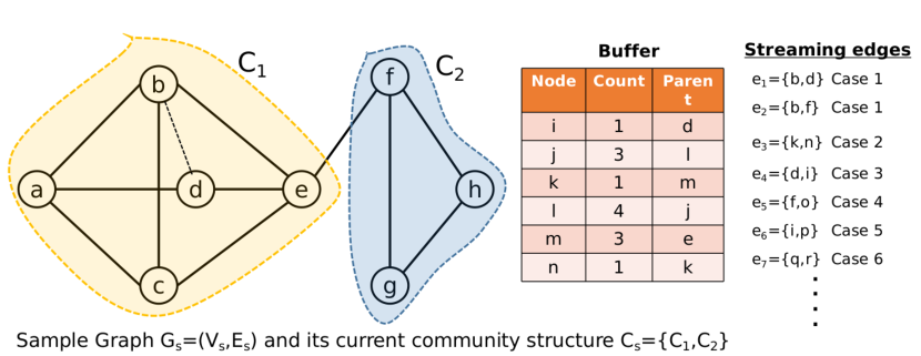
Figure 1. Toy example depicting various conditions handled by ComPAS  when a streaming edge arrives.

1 if $C_{s}(u)==C_{s}(v)$ then

2       $E_{s}=E_{s}\cup e_{t}$

3else

4       if $\Delta Q(u,C_{s}(u),C_{s}(v))<0\wedge\Delta Q(v,C_{s}(v),C_{s}(u))<0\wedge Q(\{u,v\},\{C(u),C(v)\},C^{\ast})<0$ then

5             return $V_{s},E_{s},C_{s}$

6      else

7             $w=argmax\{\Delta Q(u,C_{s}(u),C_{s}(v)),\Delta Q(v,C_{s}(v),C_{s}(u))$,

8             $Q(\{u,v\},\{C(u),C(v)\},C^{\ast})\}$

9             Move $w$ to a new community and update $C_{S}$

10             for $t\in N(w)$ do

11                   Let $t$ decide its own community Update $C_{s}$

12            

13      

return $V_{s},E_{s},C_{s}$

Function 2 $BothinSample(u,v,e_{t},V_{s},E_{s},C_{s})$

1 $\mathcal{H}_{c}[x]=\mathcal{H}_{c}[x]+1$

return $\mathcal{H}$

Function 3 $NodeinBuffer(u,\mathcal{H})$

(ii) Both $u$ and $v$ are in buffer: The only action (lines 16 - 18 of Algorithm 1) taken is that in the buffer $\mathcal{H}$, $\mathcal{H}_{c}$ entries of $u$ and $v$ are incremented by 1 which is achieved through the function $NodeinBuffer()$ (executed twice with $u$ and $v$). Example: (edge $\{k,n\}$ in Figure 1).

(iii) $u$ is in sample and $v$ is in buffer: In this case (edge $\{d,i\}$ in Figure 1) also the only action (lines 19 - 20 of Algorithm 1) taken is that in the buffer $\mathcal{H}$, $\mathcal{H}_{c}$ entry of $v$ is incremented by 1 which is implemented through the function $NodeinBuffer()$.

4.0.1. Entry of a new node:

In the three subsequent cases, at least one node is neither present in the buffer or the sample (new). This node triggers a rearrangement, whereby, another selected node is removed from the buffer to make space for the new node, and this selected node is inserted into the graph sample $G_{s}$ which further triggers a rearrangement of the sample in case it has already reached its size limit ($n$). The function $NodeisNew()$ is invoked to accomplish this task. The rearrangements that take place are described next.

Remove node from buffer: This is triggered when $\mathcal{H}$ is full and in order to make room for the new node one of the existing nodes need to be removed from $\mathcal{H}$. To this aim we preferentially remove $x$ from $\mathcal{H}$ based on the counts in $\mathcal{H}_{c}$ with the additional constraint that $\mathcal{P}(x)$ is present in $G_{s}$. We add node $x$ and edges $\{\mathcal{P}(x)$,$x$}, into $G_{s}$. This is achieved by executing the function $RemoveNodefromBuffer()$.

1 Choose $x$ preferentially from $\mathcal{H}$ $\mathcal{P}(x)\in V_{s}$

2 Remove $x$ from $\mathcal{H}$

3 $InsertNodeinSample(x,\mathcal{P}(x),V_{s},E_{s},C_{s})$

return $\mathcal{H},V_{s},E_{s},C_{s}$

Function 4 $RemoveNodefromBuffer(\mathcal{H},V_{s},E_{s},C_{s})$

Selection of node for removal from $G_{s}$: Insertion of a node into $V_{s}$ (obtained in the previous step), necessitates the removal of an existing node from the sample ($V_{s}$) to make space for the new entry. Nodes with the lowest degree in $G_{s}$ are candidates for deletion. Among these candidate nodes the one (say $x$) with the lowest clustering coefficient is then removed from the $G_{s}$ to allow insertion of a new node (selected in the previous step). Subsequently, all the edges incident on $x$ are removed from $G_{s}$. The function $CheckResizeSample()$ implements this task. Finally, the selected node ($x$) is inserted into $V_{s}$ utilizing the function $InsertNodeinSample()$, whereby, an edge $(x,\mathcal{P}(x))$ is added to $V_{s}$ and $x$ is assigned the community of $\mathcal{P}(x)$.

1 if $V_{s}==n$ then

2       Remove $m$ nodes say, $u_{1},u_{2},\cdots,u_{m}$ (and all their adjacent edges) from $G_{s}$ having lowest degree and clustering coefficient

3       for $u\in\{u_{1},u_{2},\cdots,u_{m}\}$ do

4             $C_{s}\leftarrow CommunityAfterNodeRemoval(u,C_{s})$

5      

return $V_{s},E_{s},C_{s}$

Function 5 $CheckResizeSample(V_{s},C_{s},n,m)$

1 $V_{s},E_{s},C_{s}=CheckResizeSample(V_{s},E_{s},C_{s},n,1)$

2 $V_{s}=V_{s}\cup x$

3 $E_{s}=E_{s}\cup\{x,\mathcal{P}(x)\}$

4 $C_{s}(x)=C_{s}(\mathcal{P}(x))$

Update $C_{s}$ return $V_{s},E_{s},C_{s}$

Function 6 $InsertNodeinSample(x,\mathcal{P}(x),V_{s},E_{s},C_{s})$

Adjust communities after removing a node: Deletion of a node might keep the previous community structure unchanged, or break the community into smaller parts, or merge several communities together. The community structure $C_{s}$ is adjusted using $Community-AfterNodeRemoval()$ (Function 7) incrementally. In the extreme, removal of a node might render the community disconnected or broken into smaller parts which might further merge to the other existing communities Nguyen et al. (2014). Here we utilize the clique percolation method Palla et al. (2005) to handle this situation. In particular, when a vertex $v$ is removed from a community $C$, we place a 3-clique on one of its neighbors and let the clique percolate until no vertices in $C$ are discovered. Nodes discovered in each such clique percolation will form a community. We repeat this clique percolation from each of $v$’s neighbors until each member in $C$ is assigned to a community. For example, in Figure 2 when node $g$ is removed, we place a 3-clique on its neighbor $a$. Once the 3-clique starts percolating, it accumulates all nodes except $f$. Therefore, two new communities $\{a,b,c,d,e\}$ and $\{f\}$ emerge due to the deletion of $g$. In this way, we let the remaining nodes of $C$ choose their best communities to merge in.

1 Assume node $u$ and its adjacent edges are removed from $G_{s}$

2 $i=1$

3 while $N(u)\neq\phi$ do

4       $b_{i}$=Nodes found by a 3-clique percolation on $v\in N(u)$

5       if $b_{i}==\phi$ then

6             $b_{i}=\{v\}$

7      $C_{s}=C_{s}\cup b_{i}$

8       $N(u)=N(u)\setminus b_{i}$

9       $i=i+1$

10      

11Update $C_{i}$

return $C_{s}$

Function 7 $CommunityAfterNodeRemoval(u,C_{s})$

We now proceed to discuss the remaining cases.
(iv) $u$ is in sample and $v$ is new: In this case (handled by lines 21 - 22 in Algorithm 1) $v$ is inserted into the buffer $\mathcal{H}$ if $\mathcal{H}$ is not full. Otherwise its insertion triggers rearrangements of $\mathcal{H}$ and subsequently $V_{s}$. We use $NodeisNew()$ to accomplish this task.

(v) $u$ is in buffer and $v$ is new: In this case (edge $\{m,p\}$ in Figure 1), we increment the counter corresponding to $u$ and attempt to insert $v$ into $\mathcal{H}$ using the function $NodeisNew()$.

1 if $\mathcal{H}$ is full then

2       $RemoveNodefromBuffer(\mathcal{H},V_{s},E_{s},C_{s})$

3      

4Insert u in $\mathcal{H}$

5 $\mathcal{H}_{c}[u]=1$

6 $\mathcal{H}_{p}[u]=v$

7

return $\mathcal{H},V_{s},E_{s},C_{s}$

Function 8 $NodeisNew(u,v,\mathcal{H},V_{s},E_{s},C_{s})$

(vi) Both $u$ and $v$ are new: In this case we attempt to insert both $u$ and $v$ to the buffer by executing the function $NodeisNew()$.

Summarizing, the algorithm continuously increases the proportion of high fidelity nodes and improves the community structure by the following actions – (a) delaying the insertion of a node to the sample allows for determining the importance of a node.
(b) removal of low clustering coefficient nodes from the sample ensures that only nodes with high clustering coefficient constitute the final $G_{s}$.
(c) since all the actions are aimed at improving modularity at every iteration, the final $G_{s}$ potentially will have well-separated community structure.

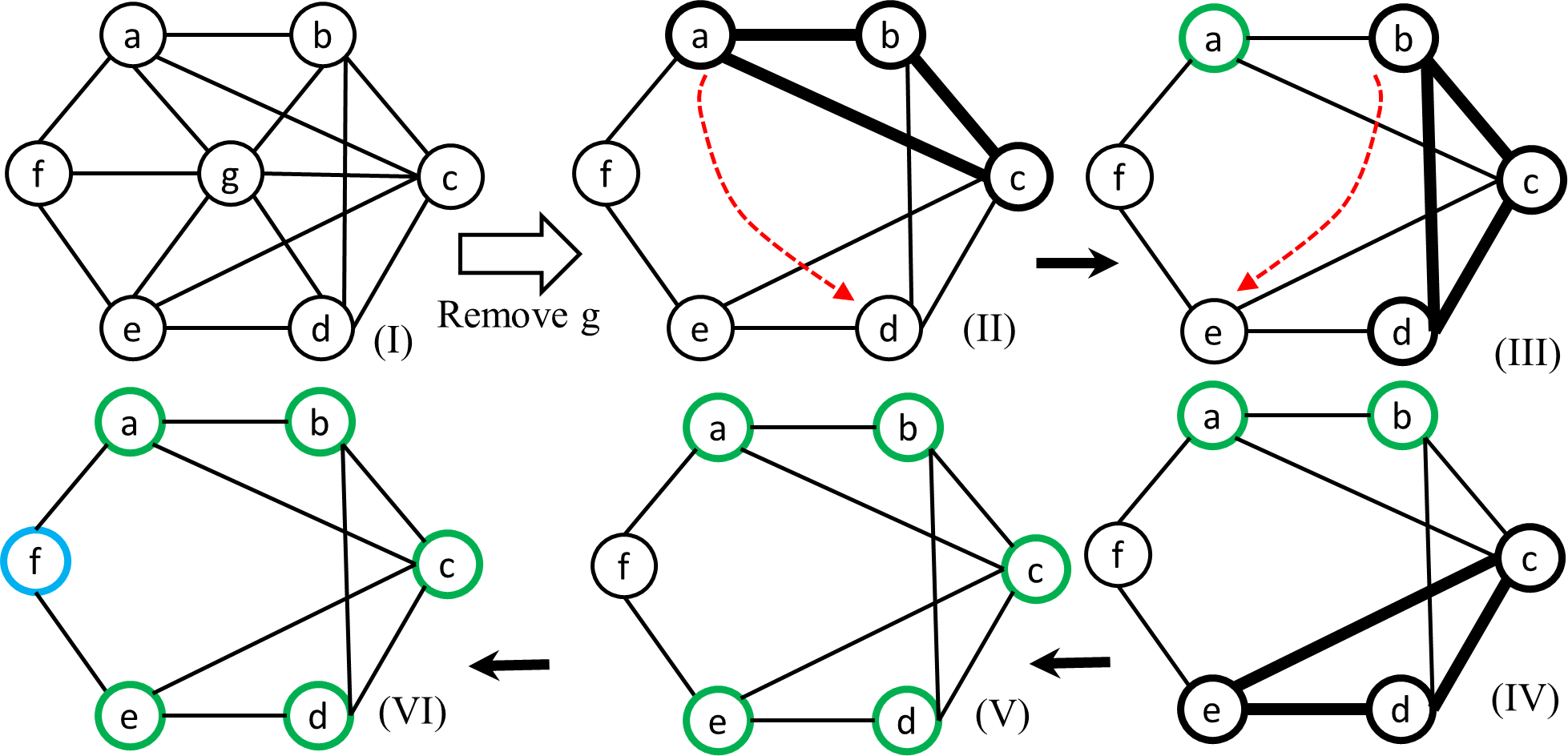
Figure 2. Illustrative example of 3-clique percolation. Once node $g$ is removed, a 3-clique is placed on node $a$. The clique percolates and accumulates all the nodes except node $f$ which forms a singleton community along with $\{a,b,c,d,e\}$.

5. Experimental setup

In this section, we outline the baseline sampling algorithms and the datasets used in our experiments.

Sampling algorithms: We compare ComPAS  with five existing sampling methods: (i) Streaming Node (SN) Ahmed et al. (2014), (ii) Streaming Edge (SE) Ahmed et al. (2014), (iii) Streaming BFS (SBFS) Ahmed et al. (2014), (iv) PIES Ahmed et al. (2014), and (v) Green Algorithm (GA) Tong et al. (2016). The first four algorithms are exclusively designed for streaming graphs while the last one is designed for static graphs. Note that unlike ours, none of the existing methods explicitly produce a community structure as a by-product of the sampling, and thus one needs to execute community detection algorithm separately on the sample to obtain the community structure. Therefore to evaluate the competing methods w.r.t how the underlying community structure in the sample corresponds to that of the original graph, for SN, SE, SBFS and PIES we run the Louvain algorithm Blondel et al. (2008) on each individual sample and detect the communities. In case of GA, we consider the aggregated graph and run GA to obtain the sample, and further run Louvain algorithm on the sample to detect the community structure. Note that although the use of aggregated graph allows GA to leverage considerably more information about the graph structure, we use it as a strict baseline in this study.

Table 1. Datasets used for evaluation.

Dataset Facebook arxiv hep-th Youtube Dblp LFR # Nodes 63,731 22,908 1,134,890 317,080 25,000 # Edges 817,035 2,444,798 2,987,624 1,049,866 254,402

Datasets: We perform our experiments on the following five graphs (the first two are streaming and last three are static):
(i) Facebook: An undirected graph where nodes (63,731) are users, and edges (817,035) are friendship links that are time-stamped.
(ii) arxiv hep-th: Here nodes (22,908) are authors of arXiv’s High Energy Physics papers and an edge exists between two authors if they have co-authored a paper; edges (2,444,798) are time-stamped by the publication date.
(iii) Youtube: Here nodes (1,134,890) represent Youtube users and edges (2,987,624) represent friendship.
(iv) dblp: This dataset consists of authors indexed in DBLP. The graph is same as arxiv hep-th (317,080 nodes and 1,049,866 edges).
(v) LFR Lancichinetti et al. (2008): This is a synthetic graph with underlying community structure implanted into it. We construct the graph with 25,000 nodes, 254,402 edges and 1,834 communities.
Since the last three graphs are static, we consider that each edge arrives in a pre-decided (random) order, i.e., each edge has a (discrete) time of arrival. The edge ordering, as we shall see, does not influence the inferences drawn from the results (Section 6). Moreover, since the first four graphs do not have any underlying ground-truth community structure, we run Louvain algorithm on the aggregated graph and obtain the disjoint community structure. This community structure is the best possible output that we can expect from our incremental modularity maximization method, and therefore serves as the ground-truth. The details of the datasets are summarized in Table 1.

6. Evaluation

Table 2. Summary of the $D$-statistics (the lower, the better) values of the topological measures for all the datasets. For Youtube we present all the results, while for the rest we provide the average $D$-statistics and standard deviation (SD). Detailed results on other datasets can be found in si (2017). ComPAS truns out to be the second best algorithm after GA (the most informed static graph sampling algorithm for which the sample is obtained from the aggregated graph and Louvain is run on the sample, thus serving as the strict baseline). Top two values for each average result is highlighted.

Algorithm Youtube Facebook dblp LFR hep-th ID EI AD FOMD TPR EX CR CON NC AODF MODF FODF MOD Avg,SD Avg,SD Avg,SD Avg,SD Avg,SD ComPAS 0.063 0.051 0.078 0.057 0.227 0.082 0.054 0.091 0.260 0.073 0.201 0.121 0.052 0.10,0.07 0.17,0.09 0.16,0.10 0.18,0.06 0.10,0.03 SN 0.164 0.171 0.471 0.061 0.542 0.581 0.112 0.265 0.064 0.157 0.182 0.092 0.216 0.23,0.17 0.33,0.17 0.29,0.20 0.27,0.07 0.26,0.04 SE 0.257 0.244 0.241 0.501 0.281 0.098 0.287 0.087 0.151 0.097 0.246 0.093 0.198 0.21,0.11 0.27,0.11 0.25,0.14 0.32,0.08 0.29,0.06 SBFS 0.126 0.131 0.172 0.106 0.454 0.145 0.056 0.165 0.045 0.257 0.108 0.076 0.181 0.15,0.10 0.26,0.09 0.24,0.10 0.25,0.09 0.26,0.04 PIES 0.234 0.241 0.252 0.190 0.409 0.042 0.051 0.049 0.061 0.157 0.042 0.053 0.121 0.14,0.10 0.29,0.06 0.24,0.07 0.26.0.05 0.21,0.05 GA 0.156 0.055 0.065 0.053 0.267 0.066 0.076 0.053 0.085 0.150 0.075 0.069 0.102 0.09,0.06 0.12,0.04 0.12,0.06 0.14,0.06 0.08,0.04

In this section, we list the standard metrics used to evaluate the goodness of the community structure, followed by a detailed comparison of the sampling algorithms.

Evaluation criteria: To measure how sampling algorithms capture the underlying community structure, we evaluate them in two ways. First we measure the quality of the obtained community structure based on the topological measures defined by Yang and Leskovec (2015). In particular, we look into four classes of quality scores - (i) based on internal connectivity: internal density (ID), edge inside (EI), average degree (AD), fraction over mean degree (FOMD), triangle participation ratio (TPR); (ii) based on external connectivity: expansion (EX), cut ratio (CR); (iii) combination of internal and external connectivity: conductance (CON), normalized cut (NC), maximum out-degree fraction (MODF), average out-degree fraction (AODF), flake out-degree fraction (FODF); and (iv) based on graph model: modularity (MOD). Note, for every individual community we obtain a score, and therefore a distribution of scores (i.e., distribution of ID, EI etc.) is obtained for all the communities of a graph. We measure how similar (in terms of Kolgomorov-Smirnov $D$-statistics) these distributions are with those of the ground-truth communities. The lesser the value of D-statistics, the better the match between two distributions.

Parameter estimation: As reported in Section 4, ComPAS consists of two parameters: (i) $\alpha$ (initial fraction of nodes inserted), (ii) $n_{d}$ (length of the buffer). We observe that $D$-statistics is initially high and reduces as we increase $\alpha$ (Figures 3(a)). For low $\alpha$, the community structure obtained initially by running a community-detection algorithm (line 12 in Algorithm 1) is coarse. For larger values of $\alpha$ even though initial community structure obtained is good, it is not allowed to evolve much. Similarly, in Figure 3(b), given a small buffer size several nodes mostly arriving once would be added to the sample leading to formation of pendant vertices. As we increase the buffer size ComPAS performs better till a certain point, after which the improvement is negligible. Since we are constrained by space, we fix $n_{d}$ at $0.0075n$. Similarly $\alpha$ is set to $0.4$. We also set $n$ to $0.4|V|$ as default (see Section 6 for different values of $n$). Further note that apart from Louvain we also consider other algorithms (CNM Clauset et al. (2004), GN Girvan and Newman (2002) and Infomap Rosvall and Bergstrom (2008)) for obtaining the initial community structure. The average $D$-statistics values (calculated for LFR) across all the quality scores for Louvain, CNM, GN and Infomap are respectively 0.182, 0.191, 0.216 and 0.197. Above results indicate that the quality of the initial communities are largely independent of the algorithm used. So we stick to the most popular one - Louvain for evaluation.

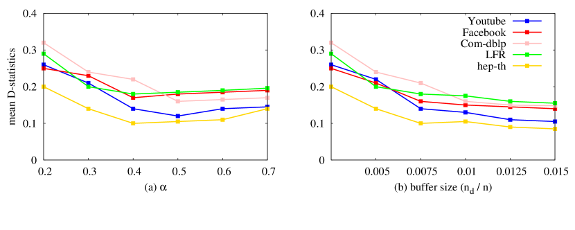
Figure 3. Average $D$-statistics value across all the topological measures for various values of $\alpha$ and $n_{d}$.

Since the nodes are labeled, as a second level of evaluation, we use the community validation metrics – Purity Manning et al. (2008), Normalized Mutual Information (NMI) Danon et al. (2005) and Adjusted Rand Index (ARI) Hubert and Arabie (1985) to measure the similarity between the ground-truth and the obtained community structures. The more the value of these metrics, the higher the similarity.

Table 3. NMI between the ground-truth and community structure obtained from individual sampling algorithms for all datasets.

Dataset	ComPAS	SN	SE	SBFS	PIES	GA
Facebook	0.52	0.34	0.28	0.41	0.48	0.61
hep-th	0.51	0.32	0.21	0.36	0.39	0.68
Youtube	0.72	0.49	0.33	0.58	0.51	0.77
dblp	0.65	0.28	0.21	0.57	0.39	0.69
LFR	0.69	0.29	0.32	0.38	0.31	0.72
Average	0.61	0.34	0.27	0.46	0.41	0.69

Comparison of sampling algorithms: We start by measuring the similarity between the obtained and the ground-truth community structures using topological measures. In Table 2 we summarize the $D$-statistics values of all the scoring functions for the Youtube dataset; for the other graphs we only present the average value (and standard deviation) across the $D$-statistics for different topological measures (detailed results on other datasets can be found in the si (2017)). Since GA is specifically designed for static graphs, we simulate GA on the aggregated network consisting of every edge that has arrived, thereby allowing it more information compared to the other (streaming) algorithms which never have the whole graph under consideration. Clearly ComPAS outperforms all the streaming algorithms across different datasets and conceivably GA performs better than ComPAS as apart from utilizing the whole network structure, it further utilizes clustering coefficient and Pagerank of each node to obtain the sample. Further we find ComPAS is the second ranked algorithm after GA with an average (over all datasets) purity, NMI and ARI of 0.74, 0.61 and 0.53 respectively (see Table 3 for NMI, details in si (2017)). Thus, ComPAS matches the ground truth community both structurally and in content.

Among the rest of the sampling algorithms PIES performs best as it is biased towards the high degree nodes but at no point attempts to maximize modularity or clustering coefficient. The limited observability of graph structure using a window in case SBFS, renders it ineffective in properly sampling high fidelity nodes. For SN since nodes are picked uniformly at random the nodes with low degreee are shortlisted. Similarly for SE, edges are picked uniformly at random and is again not inclined to pick nodes with any specific property. Hence SN and SE perform poorly in the task of preserving community structure.

Effect of edge ordering and sample size: In this section, we show that most of our inferences are valid irrespective of any edge ordering. We randomly pick one pair of edges and swap their arrival time. We repeat it for $y$% of edges (where $y$ varies between 5 and (as high as) 50) present in each aggregated graph. For each such ordering we obtain a representative sample (say $G_{y}$) and compare (average $D$-statistics) with the ground-truth community. In figure 4(a) we plot the $D$-statistics value averaged over all the scoring functions for the Youtube dataset. The plot clearly shows that the edge-ordering affects the final sample marginally (the pattern is same for other graphs).

Lastly, we present the effect of sample size ($n$) on the obtained community structure. We plot average $D$-statistics values across all the topological measures for all the algorithms on Youtube (see others in si (2017)) as a function of $n$ (Figure 4(b)). As expected, with the increase of $n$ we obtain better results. Interestingly, for ComPAS and GA, the pattern remains consistent compared to others. Moreover as we increase $n$ the divergence between their performance decreases.

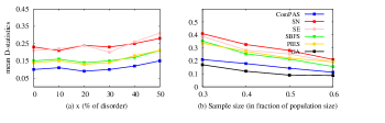
Figure 4. Average $D$-statistics across all the topological measures for (a) different edge ordering and (b) sample size ($n$) of the Youtube graph.

7. Complexity analysis

Table 4. Machine specifications used for experiments.

RAM	CPU	OS	Cores
64 GB	Intel Xeon X5690 @ 3.47 GHZ	Ubuntu 12.04 LTS	24

We perform two sets of experiments to determine the scalability of the algorithm - (i) dependence on stream size (total number of edges arriving in a single pass of the stream) and (ii) dependence on graph size ($N$). We stress that the complexity of the algorithm is (almost) linear with the size of the stream as at every step we perform certain local operations (depending on the case encountered) namely calculating modularity and clustering coefficient (calculated only for low degree nodes during deletion). As a proof of concept, we consider an LFR graph with 25000 nodes and generate a sample of size 7500 with increasing stream sizes. In figure 5(a) we plot the time required for generating the sample. We note the machine specifications in Table 4. We observe a linear behavior which corroborates our hypothesis. We further look into dependence on the size of the graph as well. In this regard we consider graphs of increasing sizes and measure the time required to obtain a sample of size 30% of the population (refer to figure 5(b)). We again observe a linear behavior for the same machine specifications noted in Table 4. The above results hence indicate that ComPAS  is scalable for large graphs as well.

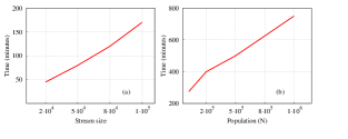
Figure 5. Execution time of ComPAS with increasing (a) stream size and (b) population size ($N$). A linear behavior is observed.

8. Insights

In this section, we present certain micro-scale insights illustrating why ComPAS outperforms the other algorithms in generating the community structure.
(i) ComPAS  admits high fidelity nodes and improves the modularity of the sample: We observe how modularity, average clustering coefficient and average degree of the sample change over time as the edges arrive in a stream (refer to figure 6(a)). All these factors increase over time. Here we report the results from the point the sample size ($n$) is reached for the first time up to the end of the stream.

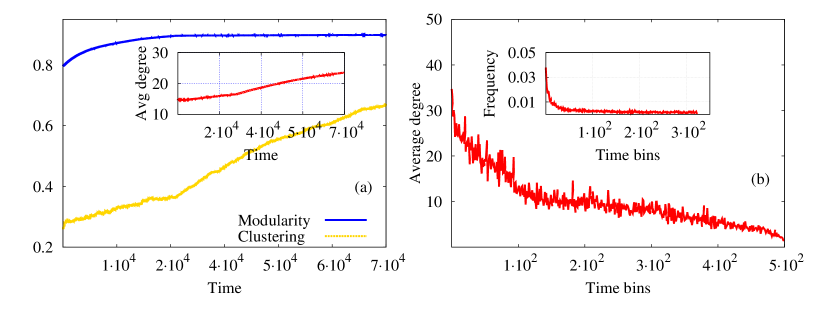
Figure 6. (a) Modularity and average clustering coefficient of the sample as it evolves over time, (inset) evolution of average degree of the sample over time.(b) Average degree of nodes in each bin (total time for streaming is divided into 500 equi-sized buckets), (inset) fraction of nodes in each bucket of the sample obtained using ComPAS. The experiment is performed on Facebook dataset.

(ii) ComPAS  retains a large fraction of intra-community edges ensuring a better community structure: We observe that intra-community edges in the sample account for $\sim$ 80% of all the edges while in the original network the corresponding value is $\sim$ 67%.
(iii) ComPAS  produces a sample that has an edge density which corresponds highly to the original graph: Note that ComPAS is node-based, and $G_{s}$ consists of only those edges which arrive after their corresponding nodes appear in $G_{s}$ - hence an efficient ComPAS would insert the nodes as early as possible. We compare the number of edges in $G_{s}$ against that in the subgraph ($\hat{G}_{s}$) induced by the sampled nodes in the original graph. We observe that on average $G_{s}$ retains $\sim 71$% of the edges of $\hat{G}_{s}$. This indicates that the insertion time of nodes (in $G_{s}$) compared to their first appearance in the stream is early as $G_{s}$ is able to retain most of the possible edges.
(iv) ComPAS samples high fidelity nodes uniformly over the time stretch: ComPAS  samples more high fidelity nodes in time stretches where such nodes appear more frequently compared to the other stretches. To this purpose we split the stream into a set of buckets and a node is placed into a bucket based on the time it first arrived and calculate the average degree of each bucket (refer to figure 6(b)). We observe that the average degree drops as we move from the first toward the subsequent buckets. We then consider the sample obtained from ComPAS and calculate the fraction of sampled nodes in each bucket (figure 6(b)(inset)). We observe a similar pattern indicating that ComPAS  is not only able to sample the high degree nodes but the rate of sampling from each is roughly proportional to the average degree of each bucket.

9. Applications of ComPAS  in online learning

In online learning, sometimes memory is limited and it is required to train the model on limited number of instances. One of the important problems in learning is to judiciously choose the training sample set - a random sampling of edges do not produce a good representative set Werner et al. (2012).

We hypothesize that more diverse the chosen set, better would be the performance. ComPAS  is useful in such cases since it tries to sample from several communities, hence improving the diversity of the training set. To this end, we consider Wiki-Rfa West et al. (2014), a streaming signed graph in which nodes represent Wikipedia members and edges (with time-stamp) represent votes. Each vote is typically accompanied by a short comment. The task is to predict the vote (+1, -1) of an incoming edge based on the textual features – (i) word count, (ii) sentiment value, and (iii) LIWC features of the statement corresponding to the edge. Moreover, we can use certain extra features like whether the edge is an intra or inter community edge, the average degree and the clustering coefficient of the nodes connected with an edge etc. to train the model. We allow training instances to be included till a certain time period $t$ (first 75% of the edges are allowed to enter) and run the sampling algorithms in parallel. However not all instances can be considered for training due to the memory constraint. We assume $n$, the sample size as the allowed training size and obtain sampled training set from individual sampling algorithms. The size of the network is 4000 and that of the sample size is 1200 which is 30% of the population. We train SVM with linear kernel (see si (2017) for other classifiers) on each sampled training set, and predict the labels (votes) of those instances coming after $t$. Table 5 shows that GA and ComPAS perform the best in terms of AUC and F-Score. This once again emphasizes that ComPAS selects most representative training instances for (restricted) online learning.

Table 5. Performance of SVM using the training set obtained from sampling methods.

	ComPAS	SN	SE	SBFS	PIES	GA
AUC	0.48	0.31	0.25	0.28	0.36	0.53
F-Score	0.61	0.35	0.28	0.31	0.43	0.64

10. Discussion

To conclude, we in this paper proposed ComPAS, a novel sampling algorithm for streaming graphs which is able to retain the community structure of the original graph. Through rigorous experimentation on real-world and synthetic graphs we showed that ComPAS  performs better than four state-of-the-art graph sampling algorithms. We also stress that the complexity of the algorithm is (almost) linear with the size of the graph as at every step we perform certain local operations (depending on the case encountered) namely calculating modularity and clustering coefficient (calculated only for low degree nodes during deletion).

One of the important problems in learning is to judiciously choose the training sample set and in this context, we demonstrated that ComPAS can be used to shortlist the training sample. We would like to point out that, although encouraging, these are initial results. A thorough analysis needs to be done on each individual use-case before strong (and universal) claims can be advocated - this would exactly be our immediate future pursuit.

11. Appendix

11.1. Proof of propositions

PROPOSITION 1. Addition of an edge to a community $c\in C$, increases its modularity if $D_{c}\leq M-1$ $($where $M=|E|)$.

Proof.

Recall the formulation of modularity as:

$$\small Q(G(V,E),C)=\sum_{c\in C}(\frac{m_{c}}{M}-\frac{D_{c}^{2}}{4M^{2}})\vspace{-2mm}$$ (1)

where $C$ is the community structure of $G$, $m_{c}$ is the total number of edges inside $c$, $D_{c}$ is the sum of degree of all the nodes inside a community $c\in C$, and $M=|E|$ is the total number of edges $G$.

From Equation 1, we see the contribution of individual community $c\in C$ in modularity as: $Q_{c}=\frac{m_{c}}{M}-\frac{D_{c}^{2}}{4M^{2}}$. where $m_{c}$ is the number of edges inside $c$, $M$ is the total number of edges in the graph, and $D_{c}$ is the sum of degrees of all the nodes in $c$.

Addition of a new edge within $c$, the $c$’s contribution of modularity becomes:

$$\small Q^{\prime}_{c}=\frac{m_{c}+1}{M+1}-\frac{(D_{c}+2)^{2}}{4(M+1)^{2}}$$

So the increase in modularity is $\Delta Q_{c}=Q^{\prime}_{c}-Q_{c}$,

$$\small\begin{split}\Delta Q_{c}=&\frac{4M^{2}-4m_{c}M^{2}-4D_{c}M^{2}-4m_{c}M+2D_{c}^{2}M+D_{c}^{2}}{4(M+1)^{2}M^{2}}\\ &\geq\frac{4M^{2}-6D_{c}M^{2}-2D_{c}M+2D_{c}^{2}M+D_{c}^{2}}{4(M+1)^{2}M^{2}}\\ &\geq\frac{(2M^{2}-2D_{c}M-D_{c})(2M-D_{c})}{4(M+1)^{2}M^{2}}\\ &\geq 0\end{split}$$

The equality holds if $D_{c}\leq M-1$. This thus implies $(2M^{2}-2D_{c}M-D_{c})\geq 0$. This proves the proposition. ∎

PROPOSITION 2. Addition of any intra-community edge into a community $c\in C$ would not split into smaller communities.

Proof.

We will prove this proposition by contradiction. Assume that once a new intra-community edge is added into $c$, it gets split into $k$ small modules, namely $X_{1}$, $X_{2}$, $\cdot$,$X_{k}$. Let $D_{X_{i}}$ and $e_{ij}$ be the total degree of nodes inside $X_{i}$ and number of edges connecting $X_{i}$ and $X_{j}$ respectively.

Recall that the contribution of $X_{i}$ in the modularity value is $Q_{X_{i}}=\frac{m_{X_{i}}}{M}-\frac{D_{X_{i}}^{2}}{4M^{2}}$. Before adding the edge, we have $Q_{c}\geq\sum_{i=1}^{k}Q_{X_{i}}$ (where $Q_{c}$ is the total modularity of community $c$), because otherwise all $X_{i}$s can be split earlier, which is not in this case. This implies that:

$$\frac{m_{c}}{M}-\frac{D_{c}^{2}}{4M^{2}}>\sum_{i=1}^{k}(\frac{m_{X_{i}}}{M}-\frac{D_{X_{i}}^{2}}{4M^{2}})$$

Since $X_{1},X_{2},\cdot,X_{k}$ are all disjoint modules of $c$, $D_{c}=\sum_{i=1}^{k}D_{X_{i}}$ and $m_{c}=\sum_{i=1}^{k}m_{X_{i}}+\sum_{i<j}e_{ij}$. This further implies that:

$$\frac{m_{c}}{M}-\sum_{i=1}^{k}\frac{m_{X_{i}}}{M}>\frac{D_{c}^{2}}{4M^{2}}-\sum_{i=1}^{k}\frac{D_{X_{i}}^{2}}{4M^{2}}$$

or,

$$\sum_{i<j}e_{ij}>\frac{\sum_{i<j}D_{X_{i}}D_{X_{j}}}{2M}$$

Without loss of generality, let us assume that the new edge is added inside $X_{1}$. Since we assume that after adding the new edge into $c$, it gets split into $k$ small modules, the modularity value should increase because of the split. Therefore, the new modularity $Q^{\prime}_{c}<\sum_{i=1}^{k}Q_{X_{i}}$. This implies that

$$\small\begin{split}\small&Q^{\prime}_{c}<\sum_{i=1}^{k}Q_{X_{i}}\\ &\Leftrightarrow\frac{\sum_{i=1}^{k}m_{X_{i}}+\sum_{i<j}e_{ij}+1}{M+1}-\frac{(\sum_{i=1}^{k}D_{X_{i}+2})^{2}}{4(M+1)^{2}}\\ &<\frac{m_{X_{1}}+1}{M+1}-\frac{(D_{X_{1}}+2)^{2}}{4(M+1)^{2}}+\sum_{i=2}^{k}(\frac{m_{X_{i}}}{M+1}-\frac{D_{X_{i}}^{2}}{4(M+1)^{2}})\\ &\Leftrightarrow\frac{\sum_{i=1}^{k}m_{X_{i}}+\sum_{i<j}e_{ij}+1}{M+1}-\frac{(\sum_{i=1}^{k}D_{X_{i}+2})^{2}}{4(M+1)^{2}}\\ &<\frac{\sum_{i=1}^{k}m_{X_{i}}+1}{M+1}-\frac{(D_{X_{1}}+2)^{2}}{4(M+1)^{2}}-\sum_{i=2}^{k}\frac{D_{X_{i}}^{2}}{4(M+1)^{2}}\\ &\Leftrightarrow\sum_{i<i}e_{ij}<\frac{\sum_{i=1}^{k}D_{X_{i}}-2D_{X_{1}}+\sum_{i<j}D_{X_{i}}D_{X_{j}}}{2(M+1)}\end{split}$$

Since $\sum_{i=1}^{k}D_{X_{i}}-2D_{X_{1}}<2M$, this implies that

$$\small\begin{split}\frac{\sum_{i<j}D_{X_{i}}D_{X_{j}}}{2M}<\sum_{i<j}e_{ij}&<\frac{\sum_{i=1}^{k}D_{X_{i}}-2D_{X_{1}}+\sum_{i\neq j}{D_{X_{i}}D_{X_{j}}}}{2(M+1)}\\ &<\frac{\sum_{i<j}D_{X_{i}}D_{X_{j}}}{2M}+1\end{split}$$

Therefore, the proposition holds. ∎

References

- (1)
- si (2017) 2017. Supplementary material (anonymized). http://bit.ly/2AusVTs. (2017). [Online; accessed 14-Nov-2017].
- Aggarwal et al. (2011) Charu C Aggarwal, Yuchen Zhao, and S Yu Philip. 2011. Outlier detection in graph streams. In ICDE. IEEE, 399–409.
- Ahmed et al. (2010) Nesreen K Ahmed, Jennifer Neville, and Ramana Kompella. 2010. Reconsidering the foundations of network sampling. In 2nd Workshop on Information in Networks.
- Ahmed et al. (2014) Nesreen K Ahmed, Jennifer Neville, and Ramana Kompella. 2014. Network sampling: From static to streaming graphs. ACM TKDD 8, 2 (2014), 7.
- Blondel et al. (2008) Vincent D Blondel, Jean-Loup Guillaume, Renaud Lambiotte, and Etienne Lefebvre. 2008. Fast unfolding of communities in large networks. Journal of statistical mechanics: theory and experiment 2008, 10 (2008), P10008.
- Clauset et al. (2004) Aaron Clauset, Mark EJ Newman, and Cristopher Moore. 2004. Finding community structure in very large networks. Physical review E 70, 6 (2004), 066111.
- Danon et al. (2005) Leon Danon, Albert Diaz-Guilera, Jordi Duch, and Alex Arenas. 2005. Comparing community structure identification. Journal of Statistical Mechanics: Theory and Experiment 2005, 09 (2005), P09008.
- De et al. (2013) Abir De, Niloy Ganguly, and Soumen Chakrabarti. 2013. Discriminative link prediction using local links, node features and community structure. In ICDM. IEEE, 1009–1018.
- Frank (1977) Ove Frank. 1977. Survey sampling in graphs. Journal of Statistical Planning and Inference 1, 3 (1977), 235–264.
- Frank (1980) Ove Frank. 1980. Sampling and inference in a population graph. International Statistical Review (1980), 33–41.
- Gile and Handcock (2010) Krista J Gile and Mark S Handcock. 2010. Respondent-driven sampling: An assessment of current methodology. Sociological methodology 40, 1 (2010), 285–327.
- Girvan and Newman (2002) Michelle Girvan and Mark EJ Newman. 2002. Community structure in social and biological networks. PNAS 99, 12 (2002), 7821–7826.
- Gjoka et al. (2010) Minas Gjoka, Maciej Kurant, Carter T Butts, and Athina Markopoulou. 2010. Walking in facebook: a case study of unbiased sampling of OSNs. In Infocom. IEEE, 1–9.
- Goodman (1961) Leo A Goodman. 1961. Snowball sampling. The annals of mathematical statistics (1961), 148–170.
- Heckathorn (1997) Douglas D Heckathorn. 1997. Respondent-driven sampling: a new approach to the study of hidden populations. Social problems 44, 2 (1997), 174–199.
- Henzinger et al. (1998) M Rauch Henzinger, Prabhakar Raghavan, and Sridhar Rajagopalan. 1998. Computing on data streams. Technical Report. Technical Note 1998-011, Digital Systems Research Center, Palo Alto, CA.
- Hubert and Arabie (1985) Lawrence Hubert and Phipps Arabie. 1985. Comparing partitions. Journal of classification 2, 1 (1985), 193–218.
- Kolascyk (2013) ED Kolascyk. 2013. Statistical Analysis of Network Data. SAMSI program on Complex networks. Boston university (2013).
- Lancichinetti et al. (2008) Andrea Lancichinetti, Santo Fortunato, and Filippo Radicchi. 2008. Benchmark graphs for testing community detection algorithms. Physical review E 78, 4 (2008), 046110.
- Leskovec and Faloutsos (2006) Jure Leskovec and Christos Faloutsos. 2006. Sampling from large graphs. In SIGKDD. ACM, 631–636.
- Leskovec et al. (2010) Jure Leskovec, Daniel Huttenlocher, and Jon Kleinberg. 2010. Predicting positive and negative links in online social networks. In WWW. ACM, 641–650.
- Li et al. (2013) Yanhua Li, Wei Chen, Yajun Wang, and Zhi-Li Zhang. 2013. Influence diffusion dynamics and influence maximization in social networks with friend and foe relationships. In WSDM. ACM, 657–666.
- Lim and Kang (2015) Yongsub Lim and U Kang. 2015. Mascot: Memory-efficient and accurate sampling for counting local triangles in graph streams. In SIGKDD. ACM, 685–694.
- Maiya and Berger-Wolf (2010) Arun S Maiya and Tanya Y Berger-Wolf. 2010. Sampling community structure. In WWW. ACM, 701–710.
- Maiya and Berger-Wolf (2011) Arun S Maiya and Tanya Y Berger-Wolf. 2011. Benefits of bias: Towards better characterization of network sampling. In SIGKDD. ACM, 105–113.
- Manning et al. (2008) Christopher D Manning, Prabhakar Raghavan, and Hinrich Schütze. 2008. Introduction to information retrieval. (2008).
- Nguyen et al. (2014) Nam P. Nguyen, Thang N. Dinh, Yilin Shen, and My T. Thai. 2014. Dynamic Social Community Detection and Its Applications. PLOS ONE 9, 4 (04 2014), 1–18.
- Palla et al. (2005) Gergely Palla, Imre Derenyi, Illes Farkas, and Tames Vicsek. 2005. Uncovering the overlapping community structure of complex networks in nature and society. Nature 435, 7043 (2005), 814–818.
- Rasti et al. (2009) Amir Hassan Rasti, Mojtaba Torkjazi, Reza Rejaie, Nick Duffield, Walter Willinger, and Daniel Stutzbach. 2009. Respondent-driven sampling for characterizing unstructured overlays. In INFOCOM. IEEE, 2701–2705.
- Ribeiro and Towsley (2010) Bruno Ribeiro and Don Towsley. 2010. Estimating and sampling graphs with multidimensional random walks. In Proceedings of the 10th ACM SIGCOMM conference on Internet measurement. ACM, 390–403.
- Rosvall and Bergstrom (2008) Martin Rosvall and Carl T Bergstrom. 2008. Maps of random walks on complex networks reveal community structure. PNAS 105, 4 (2008), 1118–1123.
- Stefani et al. (2017) Lorenzo De Stefani, Alessandro Epasto, Matteo Riondato, and Eli Upfal. 2017. TRIÈST: Counting Local and Global Triangles in Fully Dynamic Streams with Fixed Memory Size. TKDD 11, 4 (2017), 43.
- Tong et al. (2016) Chao Tong, Yu Lian, Jianwei Niu, Zhongyu Xie, and Yang Zhang. 2016. A novel green algorithm for sampling complex networks. Journal of Network and Computer Applications 59 (2016), 55–62.
- Werner et al. (2012) Jeffrey J Werner, Omry Koren, Philip Hugenholtz, Todd Z DeSantis, William A Walters, J Gregory Caporaso, Largus T Angenent, Rob Knight, and Ruth E Ley. 2012. Impact of training sets on classification of high-throughput bacterial 16s rRNA gene surveys. The ISME journal 6, 1 (2012), 94.
- West et al. (2014) Robert West, Hristo S Paskov, Jure Leskovec, and Christopher Potts. 2014. Exploiting social network structure for person-to-person sentiment analysis. arXiv preprint arXiv:1409.2450 (2014).
- Yang and Leskovec (2015) Jaewon Yang and Jure Leskovec. 2015. Defining and evaluating network communities based on ground-truth. KIAS 42, 1 (2015), 181–213.
- Ye et al. (2008) Zhenqing Ye, Songnian Hu, and Jun Yu. 2008. Adaptive clustering algorithm for community detection in complex networks. PRE 78 (Oct 2008), 046115. Issue 4. https://doi.org/10.1103/PhysRevE.78.046115