Large deviations of avalanches in the raise and peel model

Abstract

We study the large deviation functions for two quantities characterizing the avalanche dynamics in the Raise and Peel model: the number of tiles removed by avalanches and the number of global avalanches extending through the whole system. To this end, we exploit their connection to the groundstate eigenvalue of the XXZ model with twisted boundary conditions. We evaluate the cumulants of the two quantities asymptotically in the limit of the large system size. The first cumulants, the means, confirm the exact formulas conjectured from analysis of finite systems. We discuss the phase transition from critical to non-critical behaviour in the rate function of the global avalanches conditioned to an atypical values of the number of tiles removed by avalanches per unit time.

Keywords: large deviations, conformal invariance, Bethe ansatz, Temperley-Lieb algebra

1 Introduction

The large deviation theory is a way to bring concepts from the equilibrium thermodynamics to the non-equilibrium context. In particular, it is well known that in a large system in equilibrium with environment the probability distribution of a macroscopic additive quantity $X$, e.g. energy, number of particles or charge, is an exponential of the entropy, $P(X\approx x)\asymp\exp S(x)$, where the latter is normally an extensive function of $x$, i.e. $S(x)\sim Vs(x/V)$ as $V\to\infty$, where $V$ is a volume or any other additive coordinate. Below in the equations like this we use the notation $\approx$ to state that $X$ is in a small vicinity of $x$ and the sign $\asymp$ means that the ratio of logarithms of both sides tend to one as $x\to\infty$.

If we think about the time evolution of, to be specific, a stochastic system and measure an additive functional $Y_{t}$ over its trajectories, it is a common situation that at large time $t\to\infty$ the probability distribution of $Y_{t}$ takes the form

$$P(Y_{t}/t\approx y)\asymp\exp\left(-tI(y)\right).$$

This is to say that $Y_{t}$ satisfies the large deviation property with the rate function $I(y).$ Therefore, the rate function contains exactly the same information about the space-time ensemble of trajectories of a stochastic process as the specific entropy about an equilibrium system.

Alternative description of the equilibrium state can be given in terms of the Legendre transform of the entropy, the free energy $f(\mu)=-\sup_{x}(s(x)+\mu x)$, which also can be viewed as the generating function of scaled cumulants of $X.$ Similarly, the Legendre transform applied to the rate function $I(y)$ yields the scaled cumulant generating function (CGF)

$$\hat{I}(\gamma)=\sup_{y}\left(y\gamma-I(y)\right)=\lim_{t\to\infty}t^{-1}\log\mathbb{E}\left(e^{\gamma Y_{t}}\right).$$

It gives an equivalent description of time history of the system when $I(y)$ is convex.

Having its roots in Boltzmann's discovery of statistical nature of the entropy the large deviations theory was first pioneered by Cramèr [1] with application to sums of independent identically distributed random variables and then developed by Freidlin, Wentzell [2] for stochastic dynamical systems and by Donsker and Varadhan [3]-[5] for Markov processes.

One of the major applications of the theory became the stochastic systems of interacting particles, which served as toy models of non-equilibrium systems. Recently a remarkable progress was achieved for several exactly solvable models of interacting particles (for a review see [6] and references therein). Formulated in terms of Markov processes they admitted a construction of the stationary measure or even a full diagonalization of the Markov matrix by means of the matrix product ansatz or the Bethe ansatz, respectively. In this way the large deviation functions (LDF) of particle density and particle current were obtained. They served as first examples of LDF obtained for the diffusive and driven diffusive systems. Appearance of a number of exact results eventually culminated in a formulation of the macroscopic fluctuation theory, a kind of universal field theory approach to large deviations in general diffusive systems, which is not restricted solely to exactly solvable cases.

Interestingly, in some cases the finite size corrections to the scaled CGFs of particle current were conjectured to extend beyond the realm of integrable models [7],[8]. This is to say, that their functional forms are universal within the whole Edwards-Wilkinson (EW) [9] and Kardar-Parisi-Zhang (KPZ) [10] universality classes, respectively. As usual, the nature of universality depends on the symmetries or conservation laws, rather than on microscopic details of the model. In the mentioned cases it is a single hyperbolic conservation law responsible the Eulerian hydrodynamics (linear or nonlinear for EW and KPZ classes respectively). This remark is to emphasize that often the LDF is not only a characteristic of a particular model, but rather has a universal meaning within a much wider context.

The present work is devoted to large deviations in the Raise and Peel model (RPM), which is a stochastic model possessing yet another class of symmetries, very different from the previously mentioned cases, the conformal symmetry. The model was proposed in [11] as a model of interface, which moves up by local random deposition of tiles onto a substrate and moves down by spontaneous non-local avalanche-like evaporation of tiles. It was formulated in the language of representations of Temperley-Lieb (TL) algebra and dynamical rules of the model were dictated by the generator relations. It attracted significant attention due to its reach combinatorial content.

Initially the studies were concentrated on the stationary state of the process. A number of exact results on the structure of the stationary state were obtained and even more conjectures were proposed by exploiting connections between RPM and the six vertex model, XXZ model, the fully packed loop model, the O(1) loop model and alternating sign matrices (see [12, 13] and references therein). Some other predictions on space and time correlation functions in RPM were made with the use of conformal field theory [14].

Thus, most of the results on RPM obtained to date concern the properties of the stationary state, while almost no any information involving time-time correlations is yet available. In contrast, in the present paper we study the time evolution of the model, concentrating on the characteristics of the avalanche dynamics. We study the joint large deviations of two time integrated quantities: the number $\mathcal{N}_{t}^{\lozenge}$ of all tiles removed within the avalanches by given time $t$ and the total number $\mathcal{N}_{t}^{\circlearrowleft}$ of global avalanches, those which extend over the whole system. Using the mapping of the RPM to the XXZ quantum chain we obtain the largest eigenvalue of Markov matrix, deformed by inclusion of two parameters responsible for counting the mentioned quantities. This deformation gives the meaning of the generating function of joint scaled cumulants of $\mathcal{N}_{t}^{\lozenge}$ and $\mathcal{N}_{t}^{\circlearrowleft}$ to the largest eigenvalue. By applying the Legendre transform to this function we obtain the joint rate function for the two quantities. The result is obtained in the thermodynamic limit in two leading orders in the system size. The leading order, the thermodynamic value of the eigenvalue obtained, is responsible for the distribution of $\mathcal{N}_{t}^{\lozenge}$ in the thermodynamic limit. Similarly to the thermodynamic value of free energy of two-dimensional vertex models, this quantity is specific for the particular model. The next to the leading finite size correction contains information about the distribution of $\mathcal{N}_{t}^{\circlearrowleft}$, the corrections to the distribution of $\mathcal{N}_{t}^{\lozenge}$ and the mutual dependence of the two quantities. Unlike the leading order, this correction is predicted by the conformal field theory, and thus is expected to be universal to some extent. Our result allow us to obtain the exact (within the two leading orders) cumulants of both $\mathcal{N}_{t}^{\lozenge}$ and $\mathcal{N}_{t}^{\circlearrowleft}$. The cumulants of the first order, the mean, can also be obtained from averaging over the stationary states. Our results confirm the finite size formulas conjectured from the analysis of the stationary states of finite systems. The higher order cumulants are purely dynamical quantities, which are obtained first time in the present paper. We also study the asymptotics of the rate function obtained and discuss the phase transition from critical to non-critical phase observed in the large deviation functions of $\mathcal{N}_{t}^{\circlearrowleft}$ conditioned to an atypical value of the time average $\mathcal{N}_{t}^{\lozenge}/t$.

The article is organized as follows. In Section 2 we remind the basics about the Temeperley-Lieb algebra and the Periodic Temperley-Lieb algebra and formulate the Raise and Peel model defining its Markov generator in terms of the generators of the Periodic Temperley-Lieb algebra. Then we describe the R-matrix representations of the Periodic Temperley-Lieb algebra, rewrite the stochastic generator in terms of XXZ Hamiltonian with the twist and anisotropy parameters fixed at stochastic point and describe its diagonalization by the Bethe ansatz. In the last subsection of this section we discuss the stationary state of the Raise and Peel model and state two conjectures about the time averages of $\mathcal{N}_{t}^{\lozenge}$ and $\mathcal{N}_{t}^{\circlearrowleft}$. In Section 3 we introduce a non-stochastic deformation of the Markov generator, which describes an evolution of the joint moment generating function of the quantities of interest, and relate it to the Hamiltonian of XXZ chain with the twist and anisotropy parameters taking generic values. We survey the formulas for the groundstate eigenvalue of the XXZ Hamiltonian in the thermodynamic limit and for the finite size corrections to it and then reinterpret them in terms of scaled cumulant generating function of $\mathcal{N}_{t}^{\lozenge}$ and $\mathcal{N}_{t}^{\circlearrowleft}$. The end of this section contains main results of the article. In Section 4 we discuss and interpret the results obtained and mention some unsolved problems. The explicit values and asymptotics of integrals and sums used for our analysis are listed in A.

2 Raise and Peel model, Temperley-Lieb algebra and XXZ chain

2.1 Temperley-Lieb algebra

The dynamical rules of the RPM are imposed by a structure of the Temperley-Lieb (TL) algebra. In the present paper we deal with the RPM on the periodic lattice of even size $L$. It is defined in terms of the periodic TL algebra $PTL_{L}$ [15] generated by $L$ operators $e_{1},\dots,e_{L}$ satisfying the usual TL relations

$$e_{i}^{2} = 2_{q}e_{i},$$ (1)

$$e_{i}e_{i\pm 1}e_{i} = e_{i},$$ (2)

$$e_{i}e_{j} = e_{j}e_{i},\quad\left|i-j\right|>1,$$ (3)

where $i,j=1,\dots,L\,\,(\mbox{mod}\,\,L)$, which means that we impose periodicity condition $e_{L+1}\equiv e_{1}$. The coefficient in (1) is the algebra coefficient $2_{q}=q+q^{-1}$ parametrized by $q\in\mathbb{C}\setminus\{0\}$. The periodic Temperley-Lieb algebra is infinite dimensional. For our purposes we need its (still infinite dimensional) quotient algebra by relations

$$J_{L}I_{L}J_{L}=\kappa J_{L},\qquad I_{L}J_{L}I_{L}=\kappa I_{L},$$ (4)

where

$$I_{L}=e_{2}e_{4}\dots e_{L},\qquad J_{L}=e_{1}e_{3}\dots e_{L-1}$$ (5)

are the (unnormalized) projectors, and $\kappa\in\mathbb{C}\setminus\{0\}$ is yet another algebra parameter.

In the following we consider a Markov process on a finite dimensional state space with states represented by monomials from the left ideal $\mathcal{J}_{L}$ of the quotient algebra (1–4) generated by $J_{L}$ (equivalently one can consider the ideal $\mathcal{I}_{L}$ generated by $I_{L}$). Specifically, we choose the monomial $J_{L}$ from (5) to be an initial state. We call it substrate. The other states are obtained by any sequence of the generators acting on $J_{L}$ from the left.

Two different states are represented by two nonequivalent monomials, where by nonequivalent we mean that they can not be reduced to one another by applying relations (1-4). Altogether one finds ${L\choose L/2}$ states in the ideal $\mathcal{J}_{L}$. Note that an application of relations (1), (4) also yields the numerical coefficients, which are the integer powers of $2_{q}$ and $\kappa.$ We ignore them at the moment and will come back to them later, when they will play a role of corresponding transition rates of RPM.

Before going to the dynamics of the process let us give a pictorial representation to monomials from $PTL_{L}$. A rhombic tile with a diagonal of length two is associated with every generator $e_{i}$. The number $i$ refers to the horizontal position of the center of the tile in the vertical strip of width $L$. The periodicity implies that the strip is wrapped around the cylinder. Then the picture representing any monomial from the ideal is obtained by adding tiles onto the substrate $J_{L}$ shown in fig.1 in the same order as the generators enter into the monomial.

Figure 1: The substrate $J_{L}$ of width $L=8$. The cylinder is cut along vertical line at horizontal position $0$.

The tiles are placed from above to the lowest possible position that respects the boundaries of the other tiles. Conversely, to reconstruct a monomial from the picture one has to read the generators off the tiles going from left to right and from top to bottom (see examples in figures 2-4).

Figure 2: Action of two generators $e_{2}$ (left dropping tile) and $e_{4}$ (right dropping tile) on the state $e_{2}J_{6}$ results (up to numeric factor $2_{q}$) in configuration $e_{2}e_{4}J_{6}$

Figure 3: Action of generator $e_{2}$ on the state $e_{4}(e_{3}e_{5})(e_{2}e_{4}e_{6})J_{6}$ results in a stable configuration $(e_{2}e_{4}e_{6})J_{6}$. Here relation (1) was applied two times causing avalanche of a size $4$ (we include dropping tile in counting the number of erased tiles). In general, application of (1) $k$ times causes avalanche of a size $2k$.

Figure 4: Action of generator $e_{1}$ on the state $e_{4}(e_{3}e_{5})(e_{2}e_{4}e_{6})J_{6}$ resulting in a global avalanche in the system of size $L=6$. Algebraically we have $e_{1}\times e_{4}(e_{3}e_{5})(e_{2}e_{4}e_{6})J_{6}=e_{4}J_{L}I_{L}J_{L}=\kappa e_{4}J_{L}$, where we use commutativity (3) on the first step and eq.(4) on the second. Pictorially, the addition of the tile corresponding to $e_{1}$ completes two full layers of tiles, which are then removed. The removal of the two layers is interpreted as the global avalanche of size $L$.

An addition of a new tile produces a configuration, which can be either unstable (reducible) or stable (irreducible), i.e. the number of tiles in the system can or can not be reduced by application of relations (1-4) respectively. Namely, a configuration remains stable, when the tile comes to a downward corner, the valley – see action of $e_{4}$ in fig.2. In contrast, when the tile is placed onto an upward corner, the peak, it should be simply removed according to (1) – see action of $e_{2}$ in fig.2. The latter event is treated as a reflection of the tile. If the tile comes neither to a valley nor to a peak, it is on the slope of a ``mountain'', which suggests, that the relation (2) is to be applied. Successive applications of this relation cause an upward avalanche, which peels a one tile thick strip off the surface of the ``mountain'' at the level of arrival of the tile and above – see fig.3. In addition, if the two full layers of tiles have been completed on top of the substrate, they should be removed according to (4). An example of such a global avalanche is shown in fig.4. Note that all the above transformations preserve tiles at the level of substrate. All the changes are limited to the half-strip above the horizontal mid-line of the substrate, which we refer to as zero level. The upper boundary of a stable configuration is a closed broken line, touching the substrate at least once and wrapped around the cylinder. Similar representation for usual (non-periodic) TL algebra, suggests that an upper boundary of a stable configurations is a Dyck path that starts and ends at zero level, staying in the upper half-strip in-between. Hence, this representation is known as the Dyck path representation. By analogy we adopt the term periodic Dyck path representation also for the periodic case.

2.2 Raise and peel model

Now we are in a position to formulate the dynamics of RPM in terms of tiles falling onto the substrate. The continuous time Markov process starting from the substrate is defined as follows. The system is supplied with $L$ independent Poissonian clocks at each integer horizontal position $i=1,\dots,L$, which ring after exponentially distributed waiting time $\mathbb{P}(t_{i}>\tau)=e^{-\tau}$. When the clock at position $i$ has rang a tile falls down from above onto a current configuration at the position $i$. In terms of the algebra the monomial corresponding to the system configuration is multiplied by $e_{i}$. The subsequent processes is the reduction of the configuration specified by relations (1-4). Namely, if the tile comes to a peak it is rejected and disappears. If it comes to a valley it stays there with a single exception of the tile having completed two full layers of tiles on top of the substrate. In the latter case, the two layers are removed. This process affects the whole system and, hence, is referred to as global avalanche. Also, when the tile comes to the slope, it causes the local avalanche, which starts going up the mountain, peeling off the one-tile-thick layer, and continues in the same direction up to the moment when it reaches the same vertical level as it started from. All these processes are instantaneous in the Poissonian time scale.

For a general continuous time Markov process the stochastic evolution of configuration $C(t)$ of the system can be characterized by the dependence of the expectation $\mathbb{E}f(C(t))$ of an arbitrary function $f(C(t))$ on time $t$. This time dependence can be translated to the time dependence of the function itself

$$\mathbb{E}f(C(t))=\mathbb{E}_{\mathbb{P}_{0}}f_{t}(C),$$ (6)

where the expectation in the rhs is with respect to the initial probability measure $\mathbb{P}_{0}(C):=\mathrm{Prob}(C(t=0)=C)$. The time dependence of function $f_{t}(C)$ is governed by the backward Kolmogorov equation

$$\partial_{t}f_{t}(C)=\mathcal{L}f_{t}(C),$$ (7)

subject to initial conditions $f_{0}(C)=f(C)$, where the action of backward generator $\mathcal{L}$ is defined by

$$\mathcal{L}f(C)=\sum_{\{C^{\prime}\}}u_{C,C^{\prime}}(f(C^{\prime})-f(C)),$$ (8)

with $u_{C,C^{\prime}}$ being the transition rates from $C$ to $C^{\prime}$ and the sum is over the set of all stable configurations. In particular, taking the function $f(C^{\prime})=\delta_{C^{\prime},C}$ and evaluating the expectation of (7) we obtain the forward equation for the probability $\mathbb{P}_{t}(C)=\mathrm{Prob}(C(t)=C)=\mathbb{E}\delta_{C(t),C}$

$$\partial_{t}\mathbb{P}_{t}(C)=\mathcal{L}^{*}\mathbb{P}_{t}(C):=\sum_{\{C^{\prime}\}}(u_{C^{\prime},C}\mathbb{P}_{t}(C^{\prime})-u_{C,C^{\prime}}\mathbb{P}_{t}(C)).$$

Conversely, the action of the forward generator $\mathcal{L}^{*}$ on $\delta$-measures $\delta_{C}(C^{\prime})=\delta_{C,C^{\prime}}$, which form the natural basis of the space of linear functionals on functions $f(C)$, is

$$\mathcal{L}^{*}\delta_{C}=\sum_{\{C^{\prime}\}}u_{C,C^{\prime}}(\delta_{C^{\prime}}-\delta_{C}).$$ (9)

In the case of RPM the space of linear functionals can be naturally identified with $\mathcal{J}_{L}$. Then the linear operator $\mathcal{L}^{*}$ can be realized within the ideal $\mathcal{J}_{L}$ as an operator of multiplication by an element

$$\mathcal{L}^{*}=\sum_{i=1}^{L}(e_{i}-1).$$ (10)

Indeed, for every monomial $m_{C}$ representing a stable configuration $C$ we have $\mathcal{L}^{*}m_{C}=\sum_{\{C^{\prime}\}}(m_{C^{\prime}}-m_{C})$, where $m_{C^{\prime}}=e_{i}m_{C}$ for $i=1,\dots,L$. This exactly coincides with (9) given the nonzero rates are $u_{C,C^{\prime}}=1$ and the reduction of $e_{i}m_{C}$ to its stable form yields no any numeric coefficients. As it was mentioned above, an application of the relations (1-4) yields integer powers of parameters $\kappa$ and $2_{q}$. Therefore to maintain the stochasticity we have to choose the parameters to be

$$\kappa=1,\,\,\,q=e^{i\pi/3}.$$ (11)

Remark 1.

As was discussed, the functions on configurations and the probability distributions, aka linear functionals on them, are dual to each other. The Markov process can be described in terms of time-dependence of either of them, which in turn is defined by backward or forward generators respectively. The readers used to the language of quantum mechanics can define the ``state vector''

$$\left|P_{t}\right\rangle=\sum_{\{C\}}\mathbb{P}_{t}(C)m_{C}=\sum_{\{C\}}\mathbb{P}_{0}(C)m_{C}(t)$$

from $\mathcal{J}_{L},$ whose evolution can be attributed either to time dependence of coordinates or that of the basis vectors defined by $\mathcal{L}$ or $\mathcal{L}^{*}$, respectively.

To conclude the formulation of RPM we note that there are two other pictorial representations of the TL algebra in terms of links and in terms of particles, which can be useful for visualizing the algebraic relations and the dynamics of the model. For the link presentation we refer the reader to [12]. The particle representation will be briefly discussed later in Section 4 within the discussion of our results.

2.3 R-matrix representation

The algebraic construction we have been discussing so far is not very useful for analytic calculations. For practical purposes it is more convenient to work with $R$-matrix representation of PTL algebra. We consider the representation of $PTL_{L}$ on the space $\mathcal{H}=V^{\otimes L}$ obtained by tensoring $L$ copies of $V=\mathbb{C}^{2}.$ Specifically, we use the matrix

$$\check{R}:=\left(\begin{array}[]{cccc}q&0&0&0\\ 0&0&u^{-1}&0\\ 0&u&q-q^{-1}&0\\ 0&0&0&q\end{array}\right)$$

depending on the deformation and twist parameters $q,u\in\mathbb{C}$, which obeys a quadratic relation known as the Hecke condition

$$\check{R}^{2}=\boldsymbol{1}+(q-q^{-1})\check{R}.$$ (12)

The matrix can be thought of as a representation of an operator acting in the tensor product of two two-dimensional spaces $V\otimes V$. To construct a generalization acting on the whole space $\mathcal{H}$ we introduce operator

$$\check{R}_{i,i+1}=\boldsymbol{1}_{1}\otimes\cdots\otimes\boldsymbol{1}_{i-1}\otimes\check{R}\otimes\mathbf{1}_{i+2}\otimes\cdots\otimes\boldsymbol{1}_{L}$$

that acts as an identity operator on all the components of the tensor product except the spaces with numbers $i,i+1\,\,\,\mathrm{mod}\,\,\,L$ intertwined by $\check{R}.$ In addition to the Hecke relation these operators also satisfy the braid relation

$$\check{R}_{i,i+1}\check{R}_{i+1,i+2}\check{R}_{i,i+1}=\check{R}_{i+1,i+2}\check{R}_{i,i+1}\check{R}_{i+1,i+2},$$ (13)

where all the sub-indices should be read $\mathrm{mod}\,\,L$, while operators $\check{R}_{i,i+1}$and $\check{R}_{j,j+1}$ acting non-trivially on spaces, which are not next to each other, commute

$$\check{R}_{i,i+1}\check{R}_{j,j+1}=\check{R}_{j,j+1}\check{R}_{i,i+1},\,\,\,|i-j|>1\,\,\mbox{(mod $L$).}$$ (14)

To define the representation $\rho:PTL_{L}\to\mathrm{End}\,\mathcal{H}$ as an algebra homomorphism from $PTL_{L}$ to linear transformations of $\mathcal{H},$ we assign

$$\rho(e_{i})=q\mathbf{1}-\check{R}_{i,i+1}.$$

With this prescription it is not difficult to check that relations (12-14) are indeed equivalent to relations (1-3) between generators of $PTL_{L}$ respectively. A bit more involved calculations show that relation (4) also holds with

$$\kappa=\left(u^{L/2}+u^{-L/2}\right)^{2}$$ (15)

We conclude this subsection by writing down the form that the forward Markov generator (10) takes in the $R$-matrix representation

$$\rho(\mathcal{L}^{*})=\sum_{i=1}^{L}\left[(q-1)\mathbf{1}-\check{R}_{i,i+1}\right].$$

Despite it represents the stochastic operator, the basis this matrix is written in is the spin basis rather than the basis of RPM configurations. This is why the matrix $\rho(\mathcal{L}^{*})$ is not stochastic even when the stochasticity condition (11) is satisfied.

2.4 XXZ model

The $R$-matrix form of the forward generator takes the familiar form of the Hamiltonian of quantum XXZ chain if we rewrite the $R$-matrices in terms of $\sigma-$matrices

$$\sigma^{+}=\left(\begin{array}[]{cc}0&1\\ 0&0\end{array}\right),\,\,\,\sigma^{-}=\left(\begin{array}[]{cc}0&0\\ 1&0\end{array}\right),\,\,\,\sigma^{z}=\left(\begin{array}[]{cc}1&0\\ 0&-1\end{array}\right).$$

The matrix representing generator $e_{i}$ can be expanded into a sum of tensor products of such matrices acting non-trivially on the pair of spaces $V_{i}\otimes V_{i+1}$ from $\mathcal{H}$

$$\rho(e_{i})=\left[u\sigma_{i}^{+}\otimes\sigma_{i+1}^{-}+u^{-1}\sigma_{i}^{-}\otimes\sigma_{i+1}^{+}-\frac{\cos\gamma}{2}(\sigma_{i}^{z}\otimes\sigma_{i+1}^{z}-\mathbf{1}\otimes\mathbf{1})+\frac{\mathrm{i}\sin\gamma}{2}(\sigma_{i}^{z}\otimes\mathbf{1}-\boldsymbol{1}\otimes\sigma_{i+1}^{z})\right],$$

where the sub-indices of $\sigma-$matrices index the tensor components of $\mathcal{H}$, where these matrices act, and we introduce new notation $\gamma$ by

$$\cos\gamma=\frac{2_{q}}{2},\qquad\sin\gamma=\frac{q-q^{-1}}{2\mathrm{i}}.$$ (16)

In this form it is easy to see that the forward generator of Markov process is represented by

$$\rho(\mathcal{L}^{*})=-\left(2-\cos\gamma\right)L/2-H_{XXZ}^{\Delta,u},$$ (17)

where

$$H_{XXZ}^{\Delta,u}=-\sum_{i=1}^{L}\left[u\sigma_{i}^{+}\otimes\sigma_{i+1}^{-}+u^{-1}\sigma_{i}^{-}\otimes\sigma_{i+1}^{+}+\frac{\Delta}{2}\sigma_{i}^{z}\otimes\sigma_{i+1}^{z}\right]$$ (18)

is the Hamiltonian of the antiferromagnetic Heisenberg quantum chain of $L$ spins 1/2 with anisotropy

$$\Delta=-\cos\gamma$$ (19)

and the twist parameter $u$, which accounts for the effect of magnetic flux through the ring when $|u|=1$. In case $\left|u\right|\neq 1$, the latter breaks the left-right symmetry of the model making the Hamiltonian non-Hermitian. Here we imply the periodic boundary conditions $\left\{\sigma_{L+1}^{\pm}=\sigma_{1}^{\pm},\,\sigma_{L+1}^{z}=\sigma_{1}^{z}\right\}$. Alternatively, by a unitary transformation the parameter $u$ can be transferred from the Hamiltonian to twisted boundary conditions [16]:

$$\left\{\sigma_{L+1}^{\pm}=u^{\pm L}\sigma_{1}^{\pm},\,\,\,\sigma_{L+1}^{z}=\sigma_{1}^{z}\right\}.$$

To describe the relation between RPM and XXZ model precisely we should specify the subspace of $\mathcal{H}$ that is isomorphic to $\mathcal{J}_{L}$. As is well known [16] the XXZ Hamiltonian (18) commutes with an operator of the total spin projection $S_{z}=\frac{1}{2}\sum_{i=1}^{L}\sigma_{i}^{z}$. This is why the invariant subspaces of $H_{XXZ}^{\Delta,u}$ are indexed by values of the total projection $S_{z}\in\{-L/2,\dots L/2\}$. In particular, the periodic Dyck path representation is isomorphic to the subspace with $S_{z}=0$.

2.5 Bethe ansatz

In the following we will be interested in eigenvalues of the generators of RPM $\mathcal{L}^{*}$ and $\mathcal{L}$, which are related to those from the $S_{z}=0$ sector of $H_{XXZ}^{\Delta,u}$ due to (17).

As is well known, the XXZ Hamiltonian is diagonalized in each sector of a given total spin projection $S_{z}=L/2-m$, $m=0,1,\dots,L$, by the Bethe eigenvectors

$$\left|\boldsymbol{z}\right\rangle=\sum_{1\leq i_{1}<\dots<i_{m}\leq L}\psi(i_{1},\dots,i_{m}|\boldsymbol{z})\sigma_{i_{1}}^{-}\otimes\dots\otimes\sigma_{i_{m}}^{-}\left|\left(\begin{array}[]{c}1\\ 0\end{array}\right)\otimes\dots\otimes\left(\begin{array}[]{c}1\\ 0\end{array}\right)\right\rangle,$$

where the function

$$\psi(i_{1},\dots,i_{m}|\boldsymbol{z})=\sum_{\sigma\in S_{m}}\left(-1\right)^{\sigma}\prod_{1\leq i<j\leq m}\frac{1-2u\Delta z_{\sigma(i)}+u^{2}z_{\sigma(i)}z_{\sigma(j)}}{1-2u\Delta z_{i}+u^{2}z_{i}z_{j}}\prod_{k=1}^{m}z_{\sigma(k)}^{i_{k}}$$

is a sum over permutations $\sigma\in S_{m}$ of $m!$ terms parametrized by a particular solution $\boldsymbol{z}=(z_{1},\dots,z_{m})$ of a system of the Bethe equations

$$z_{i}^{L}=\left(-1\right)^{m-1}\prod_{j=1}^{m}\frac{1-2u\Delta z_{i}+u^{2}z_{i}z_{j}}{1-2u\Delta z_{j}+u^{2}z_{i}z_{j}},\,\,\,i=1,\dots,m.$$

Every solution defines a single eigenvector corresponding to the eigenvalue of the Hamiltonian, i.e. the energy

$$E_{XXZ}=\Delta\left(2m-\frac{L}{2}\right)-\sum_{i=1}^{m}\left[uz_{i}+\left(uz_{i}\right)^{-1}\right].$$

In general evaluation of a particular value of the energy is a difficult problem that requires finding a particular solution of the system explicitly. However, the relation

$$\Lambda^{RPM}=-E_{XXZ}-\left(2+\Delta\right)L/2,$$

between eigenvalue $\Lambda^{RPM}$ of the stochastic generators $\mathcal{L}$ and $\mathcal{L}^{*}$ and the energy $E_{XXZ}$ that follows from (17) allows one to get some immediate information relying on the stochasticity only. Specifically a generator of Markov process has a non-degenerate zero eigenvalue

$$\Lambda_{0}^{RPM}=0.$$

which is the eigenvalue with the largest real part. Thus, the minimal energy of the XXZ model in the sector $S_{z}=0$ at the stochastic point (11), i.e

$$\gamma=\pi/3,\quad\Delta=-1/2,\quad u=e^{\mathrm{2\pi i}/(3L)},$$ (20)

is $E_{XXZ}=-3L/4$, which is also the total minimum over all sectors. Remarkably, though the most of results on the energy levels of XXZ model are obtained in the thermodynamic limit $L\to\infty$, the latter one is exact for arbitrary $L$. In the following we will go beyond the stochastic point, using this value as the starting point of the large deviation analysis.

2.6 Stationary state

It was first observed by Razumov and Stroganov [17] that the ground state eigenvector of the XXZ Hamiltonian at $\Delta=-1/2$ possesses remarkable combinatorial properties. This observation was immediately reinterpreted and further developed in applying to the ground state vector of the dense $O(1)$ model [18, 19, 20] which, in turn, led to a formulation of the stochastic Raise and Peel model [11]. An extensive list of conjectures relating stationary probabilities of the RPM with enumerations of various symmetry classes of the Alternating Sign Matrices and Plane Partitions was later presented in [21, 22]. Below we formulate a pair of such conjectures. Their large scale limits will be approved later in section 3.2 (see eqs.(41),(50)).

Denote $\Psi_{L}$ a vector in the ideal $\mathcal{J}_{L}$ which corresponds to the stationary state of the RPM: $\mathcal{L}^{*}\Psi_{L}=0$. Written in the basis of the periodic Dyck paths this vector gives stationary probabilities of the stable configurations. Combinatorial properties of the stationary state are most suitably observed from $\Psi_{L}$ if it is normalized so that its smallest coefficients are equal to 1. In this case a total sum of all coefficients of $\Psi_{L}$, i.e. the probability normalization, coincides with the number of $L\times L$ half turn symmetric Alternating Sign Matrices [21]:

$$A_{\mbox{\tiny HT}}(L)=\prod_{k=0}^{L/2-1}\frac{(3k+2)!(3k)!}{(L/2+k)!^{2}}=2,10,140,\dots$$

In figure 5 we present explicit expressions for $\Psi_{L}$ for small values of $L$. One can use them to test the formula above and the conjectures given below.

Conjecture 1.[21] An average number of peaks (local maxima) as well as valleys (local minima) in the stationary state $\Psi_{L}$ equals

$$L\cdot\frac{3L^{2}}{8(L^{2}-1)}\,=\,2\cdot\mbox{$\frac{1}{2}$},\,\,4\cdot\mbox{$\frac{2}{5}$},\,\,6\cdot\mbox{$\frac{27}{70}$},\dots\quad\mbox{for $L=2,4,6,\dots$}$$

Conjecture 2. Stable configurations which do not have valleys on level $0$ and have a single valley on level $1$ (these configurations are painted red in fig.5) appear in the stationary state $\Psi_{L}$ with probability

$$\frac{3L}{4(L^{2}-1)}\,=\,\frac{1}{2},\,\,\frac{1}{5},\,\,\frac{9}{70},\dots\quad\mbox{for $L=2,4,6,\dots$}$$

From the above formulas one infers the expressions for the total number of tiles removed within the avalanches and the number of global avalanches per unit time in the large time limit:

$$\lim_{t\to\infty}\mathbb{E}\frac{\mathcal{N}_{t}^{\lozenge}}{t}=L\cdot\frac{5L^{2}-8}{8(L^{2}-1)},$$ (21)

$$\lim_{t\to\infty}\mathbb{E}\frac{\mathcal{N}_{t}^{\circlearrowleft}}{t}=\frac{3}{4}\frac{L}{L^{2}-1}.$$ (22)

Here for the first formula one notices that in the stationary state the avalanches should remove all the tiles that are not reflected, i.e. those hitting configurations everywhere except the peaks. For the second formula one observes that the states described in Conjecture 2 are precisely those which may suffer the global avalanches.

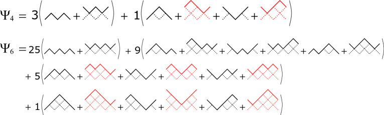
Figure 5: Stationary states of the Raise and Peel Model for $L=4$ and $L=6$.

3 Large deviations

In subsection 2.2 we discussed evaluation of expectations of functions on configurations of Markov process at fixed moment of time. They are given in terms of the solution of the backward equation (6,7), which in turn can be represented as the integral over trajectories of the process

$$\mathbb{E}f(C(t)) = \mathbb{E}_{\mathbb{P}_{0}}e^{t\mathcal{L}}f(C)$$ (23)

$$= \sum_{n,C_{0},\dots,C_{n}}f(C_{n})\int_{0\leq t_{1}\leq\dots\leq t_{n}\leq t}d\mathbb{P}_{C_{0},,\dots,C_{n}}(t_{1},\dots,t_{n}),$$ (24)

where

$$d\mathbb{P}_{C_{0},\dots,C_{n}}(t_{1},\dots,t_{n})=\mathbb{P}_{0}(C_{0})\prod_{k=0}^{n-1}u_{C_{k},C_{k+1}}e^{-\left(t_{k+1}-t_{k}\right)u_{C_{k},C_{k+1}}}dt_{k+1}$$

is the measure of the trajectories starting from initial distribution $\mathrm{Prob}(C(t=0)=C)=\mathbb{P}_{0}(C)$ at time $t_{0}=0$, passing through configurations $C_{0},\dots,C_{n}$ by time $t$ so that the jump from $C_{i-1}$to $C_{i}$ has happened within interval $[t_{i},t_{i}+dt_{i}]$ for $i=1,\dots,n$.

In similar fashion one can study the statistics of additive functionals on the system trajectories. Specifically, consider a right-continuous random (possibly multicomponent) function of time $\boldsymbol{\mathcal{N}}_{t}=(\mathcal{N}_{t;1},\dots,\mathcal{N}_{t;k})$, which initially is $\boldsymbol{\mathcal{N}}_{t=0}=(0,\dots,0)$ and changes abruptly by

$$\boldsymbol{\mathcal{N}}_{t}=\boldsymbol{\mathcal{N}}_{t-0}+\delta\boldsymbol{\mathcal{N}}_{C,C^{\prime}}$$

every time the system jumps between two configurations. The values of $\delta\boldsymbol{\mathcal{N}}{}_{C,C^{\prime}}$, fixed once for all, depend only on configurations $C$ and $C^{\prime}$ before and after the jump respectively, but not on time or history of the process. Hence, for the trajectory that has passed through configurations $C_{0},\dots,C_{n}$ by time $t$, we have $\boldsymbol{\mathcal{N}}_{t}=\delta\boldsymbol{\mathcal{N}}_{C_{0},C_{1}}+\cdots+\delta\boldsymbol{\mathcal{N}}_{C_{n-1},C_{n}}$. Therefore, the expectations of the form $\mathbb{E}\left(f(C_{t})e^{\boldsymbol{\alpha}\boldsymbol{\mathcal{N}}_{t}}\right)$, where $\boldsymbol{\alpha}=(\alpha_{1},\dots,\alpha_{k})$ is a parameter and $\boldsymbol{\alpha}\boldsymbol{\mathcal{N}}_{t}=\sum_{i}\alpha_{i}\mathcal{N}_{t;i}$, can be written in the form of integral over trajectories, similar to (24) up to the change of integration measure $d\mathbb{P}_{C_{0},,\dots,C_{n}}(t_{1},\dots,t_{n})$ to a new measure

$$d\mathbb{M}_{C_{0},\dots,C_{n}}^{\boldsymbol{\alpha}}(t_{1},\dots,t_{n})=\mathbb{P}_{0}(C_{0})\prod_{k=0}^{n-1}\left[u_{C_{k},C_{k+1}}e^{\boldsymbol{\alpha}\delta\boldsymbol{\mathcal{N}}_{C_{k},C_{k+1}}}\right]e^{-\left(t_{k+1}-t_{k}\right)u_{C_{k},C_{k+1}}}dt_{k+1}$$

obtained from the former one by assigning an additional weight $e^{\boldsymbol{\alpha}\delta\mathcal{\boldsymbol{N}}_{C_{k},C_{k+1}}}$ to every jump between two configurations. Of course, this is not a probability measure anymore, i.e. it does not have a unit normalization. Its total normalization obtained by setting $f(C)\equiv 1$ is exactly the quantity of our interest, the generating function $\mathbb{E}e^{\boldsymbol{\alpha}\boldsymbol{\mathcal{N}}_{t}}$ of joint moments of $\boldsymbol{\mathcal{N}}_{t}$. Similarly to (23) it can be written in terms of the exponential

$$\mathbb{E}e^{\boldsymbol{\alpha}\boldsymbol{\mathcal{N}}_{t}}=\mathbb{E}_{\mathbb{P}_{0}}\left(e^{t\mathcal{L}_{\boldsymbol{\alpha}}}\boldsymbol{1}\right),$$ (25)

of a new operator $\mathcal{L}_{\alpha}$,

$$\mathcal{L}_{\boldsymbol{\alpha}}f(C)=\sum_{C^{\prime}\neq C}u_{C,C^{\prime}}\left(e^{\boldsymbol{\alpha}\delta\boldsymbol{\mathcal{N}}_{C,C^{\prime}}}f(C^{\prime})-f(C)\right).$$

The main point of the large deviation theory applied to the finite state space Markov process is the observation that in the large time limit the exponential in the r.h.s. of (25) is dominated by the largest eigenvalue of the generator $\mathcal{L}_{\boldsymbol{\alpha}}$, that is to say that the scaled CGF converges to the largest eigenvalue

$$I_{\boldsymbol{\mathcal{N}}_{t}}(\boldsymbol{\alpha}):=\lim_{t\to\infty}t^{-1}\mathbb{\log E}e^{\boldsymbol{\alpha}\boldsymbol{\mathcal{N}}_{t}}=\Lambda_{0}(\boldsymbol{\alpha}).$$

Returning back to RPM we are going to analyze large deviations of two-component additive functional $\boldsymbol{\mathcal{N}}_{t}=\left(\mathcal{N}_{t}^{\circlearrowleft},\mathcal{N}_{t}^{\lozenge}\right)$ on the trajectories of the process, where

$\mathcal{N}_{t}^{\circlearrowleft}$-

the total number of global avalanches occurred in the system by the time $t$.

$\mathcal{N}_{t}^{\lozenge}$-

the total number of tiles removed from the systems during avalanches (both local and global) by the time $t$,

Following the above discussion, we would like to obtain the scaled joint CGF of $\left(N_{t}^{\circlearrowleft},\mathcal{N}_{t}^{\lozenge}\right)$, i.e. the largest eigenvalue $\Lambda(\alpha,\beta)$ of the operator $\mathcal{L}_{(\alpha,\beta)}$ obtained from the generator (8) by multiplying the off-diagonal matrix elements $u_{C,C^{\prime}}$ by $e^{\alpha\delta\mathcal{N}_{C,C^{\prime}}^{\circlearrowleft}+\beta\delta\mathcal{N}_{C,C^{\prime}}^{\lozenge}}$.

To this end, we extend the algebraic construction of the previous section to the operator $\mathcal{L}_{(\alpha,\beta)}$. First, let us rescale generators of the periodic Temperley-Lieb algebra

$$\tilde{e}_{i}:=2_{q}^{-1}e_{i},\quad\tilde{I}_{L}:=\tilde{e}_{2}\tilde{e}_{4}\dots\tilde{e}_{L},\quad\tilde{J}_{L}:=\tilde{e}_{1}\tilde{e}_{3}\dots\tilde{e}_{L-1}.$$

PTL relations (1-4) in terms of them read:

$$\tilde{e}_{i}^{2} = \tilde{e}_{i},$$ (26)

$$\tilde{e}_{i}\tilde{e}_{i\pm 1}\tilde{e}_{i} = 2_{q}^{-2}\tilde{e}_{i},$$ (27)

$$\tilde{e}_{i}\tilde{e}_{j} = \tilde{e}_{j}\tilde{e}_{i},\,\,\,\left|i-j\right|>1,$$ (28)

$$\tilde{J}_{L}\tilde{I}_{L}\tilde{J}_{L} = \kappa 2_{q}^{-L}\tilde{J}_{L},\quad\tilde{I}_{L}\tilde{J}_{L}\tilde{I}_{L}\,\,=\,\,\kappa 2_{q}^{-L}\tilde{I}_{L}.$$ (29)

Note that in this presentation nontrivial numerical factors depending on two parameters $q$ and $\kappa$ appear in relations (27) and (29) only. These two relations are just the ones responsible for removing tiles during avalanches: one-time application of (27) results in removing a pair of tiles from a configuration within a local avalanche and multiplies corresponding monomial by $2_{q}^{-2}$ ; (29) removes $L$ tiles within a single global avalanche and multiplies the monomial by $\kappa 2_{q}^{-L}$. The numeric factors enter the matrix elements of linear operators corresponding to multiplication of monomials in the ideal $\mathcal{J}_{L}$ by operators $\tilde{e}_{i}.$ In particular, if we set

$$\kappa=e^{\alpha}\,\,\,\mathrm{and\,\,\,}2_{q}^{-1}=e^{\beta},$$

the off-diagonal matrix elements of an operator

$$\mathcal{L}^{*}_{(\alpha,\beta)}=\sum_{i=1}^{L}(\tilde{e}_{i}-1),$$ (30)

will be those of the forward generator $\mathcal{L}^{*}$ of RPM multiplied by additional factors $e^{\alpha\delta\mathcal{N}_{C,C^{\prime}}^{\circlearrowleft}+\beta\delta\mathcal{N}_{C,C^{\prime}}^{\lozenge}}$, as was required. The representation of (30) in $\mathcal{H}$ is still given in terms of XXZ Hamiltonian

$$\rho\left(\mathcal{L}^{*}_{(\alpha,\beta)}\right)=-e^{\beta}H_{XXZ}^{\Delta,u}-\frac{3L}{4},$$

where the values of parameters $\Delta$ and $u$ are now away from the stochastic point (20) being related to $\alpha$ and $\beta$ by

$$u^{L/2}+u^{-L/2}=e^{\alpha/2},\,\,\,2\Delta=-e^{-\beta}.$$

With this parametrization we find the largest eigenvalue of the operator $\mathcal{L}^{*}_{(\alpha,\beta)}$, aka scaled generating function of the joint cumulants of $\mathcal{N}_{t}^{\circlearrowleft}$ and $\mathcal{N}_{t}^{\lozenge}$.

$$\Lambda_{0}(\alpha,\beta) = -e^{\beta}E_{L}^{XXZ}(\Delta,u)-\frac{3L}{4}.$$ (31)

3.1 The groundstate of XXZ Hamiltonian

Let us summarize what is known about the largest eigenvalue of twisted XXZ Hamiltonian. Here we concentrate on the thermodynamic limit $L\to\infty$ and on the values of the other parameters $\Delta$ and $u$ chosen such that the related parameters $\alpha$ and $\beta$ are finite, $\alpha,\beta\in\mathbb{R}$. This suggests that $\Delta\leq 0$ and $u=\exp\left[\mathrm{i}\varphi/L\right]$ with $\varphi$ either real, $0\leq\varphi\leq\pi$, or pure imaginary, $0\leq\mathrm{i}\varphi<\infty.$ The stochastic point corresponds to $\Delta=-1/2$ and $\varphi=2\pi/3$.

In the thermodynamic limit $E_{L}^{XXZ}(\Delta,u)$ consists of the bulk term, growing linearly in $L$ as $L\to\infty$ and finite size corrections (FSC). As anticipated from the scaling of $u$, the bulk energy per site

$$e_{\infty}(\Delta)=\lim_{L\to\infty}L^{-1}E_{L}^{XXZ}(\Delta,u),$$

depends only on $\Delta$, while $\varphi$ appears in the FSC. Their explicit expressions and methods of derivation depend on which of two regimes, gapless $|\Delta|<1$ or gapped $\Delta<-1$, is considered.

The bulk term was obtained by Yang and Yang [23, 24] in the whole range of values of $\Delta$. The FSC where analyzed in a number of papers in different contexts. Initially, a systematic method of calculation of FSC was proposed in [25] for gapped regime and extended to gapless regime in [26].

The gapless regime attracted a lot of attention in connection with conformal field theory (CFT) predictions to the free energy of 2D statistical systems. The FSC to the free energy of models like Potts model, Ashkin-Teller model, six-vertex and eight-vertex models were obtained and tested against CFT predictions (see the review [27] and references therein). These studies exploited the analogy with XXZ model at particular fixed values of twist parameter. The general formula for the groundstate energy as a function of the twist was first proposed on the basis of numerical solution of Bethe equations in [16]. It was then derived analytically from their finite size analysis in [28]. The CFT meaning of these results obtained for arbitrary twist was clarified in [29].

The gapped regime is less studied. In addition to [25] the XXZ chain with antiperiodic boundary conditions was considered [30], which corresponds to a particular value of the twist $\varphi=\pi$.

Bellow we give a brief survey of the behaviour of $e_{\infty}(\Delta)$ and of FSC for $\Delta$ and $\varphi$ in the range of interest. For the gapless phase we refer to a straightforward generalization of results of [25, 26, 28]. Note that the imaginary twist ceases the Hamiltonian from being Hermitian. The Bethe roots deviate from the real axis in this case. This deviation however is itself of order of $1/L$, assuring that the contour of roots does not encounter any singularities and all the arguments using contour integration are preserved.

In the gapped phase no any formulas for arbitrary twist were yet obtained to our knowledge. Below we give the result obtained by direct extension of techniques of [25, 31]. The detailed calculations will be presented elsewhere.

We also briefly mention the intermediate scaling regime that connects the two phases, though no finial exact results were obtained for it yet.

Gapless phase

In the gapless regime with

$$\Delta=-\cos\gamma,\,\,\gamma\in[0,\pi/2]$$

the bulk part is

$$e_{\infty}(\Delta)=\frac{\cos\gamma}{2}-\sin^{2}\gamma\,Y(\gamma)$$ (32)

given in terms of an integral

$$Y(\gamma)=\int_{-\infty}^{+\infty}\frac{dx}{\cosh\left(\pi x\right)}\frac{1}{\left[\cosh(2\gamma x)-\cos\gamma\right]}.$$ (33)

The $\varphi-$dependent FSC of order of $1/L$ are quadratic in $\varphi$

$$\lim_{L\to\infty}L\left(E_{L}^{XXZ}(\Delta,e^{\mathrm{i}\varphi/L})-Le_{\infty}(\Delta)\right)=-\frac{\pi^{2}\sin\gamma}{6\gamma}+\varphi^{2}\frac{\pi\sin\gamma}{4\gamma(\pi-\gamma)},$$ (34)

where the union of the real and imaginary domains of $\varphi\in[0,\pi]\bigcup\mathrm{i\times}[0,\infty]$ suggests that $-\infty<\varphi^{2}\leq\pi^{2}.$

Gapped phase

In the gapped phase, $\Delta<-1$ we use the parametrization

$$\Delta=-\cosh\lambda,\,\lambda\in(0,\infty).$$

In this case the groundstate is known to be asymptotically double degenerate, that is to say that the distance between the two lowest eigenstates is exponentially small in the system size and there is a finite gap to the third lowest state [32].

The expression of the bulk energy

$$e_{\infty}(\Delta)=\frac{\cosh\lambda}{2}-\sinh^{2}\lambda\tilde{Y}(\lambda)$$ (35)

includes now an infinite sum

$$\tilde{Y}(\lambda)=\frac{1}{\sinh\lambda}\sum_{m\in\mathbb{Z}}\frac{\exp(-|m|\lambda)}{\cosh m\lambda}.$$ (36)

It was shown in [24] that the functions $Y(\gamma)$ and $\tilde{Y}(\lambda)$ (and hence the two expressions of $e_{\infty}(\Delta)$) can be thought of as a continuation of one another from the real axis to the imaginary one, $\lambda=\mathrm{i}\gamma$, such that all the derivatives are continuous, while the difference is the function with essential singularity at the origin.

The FSC in the gapped regime are exponentially small in the system size, distinguishing however between the two asymptotically degenerate groundstates. Their leading term

$$E_{L}^{XXZ}(\Delta,e^{\mathrm{i}\varphi/L})-Le_{\infty}(\Delta)$$ (37)

$$\,\,\,\,\,\,\,\,\,\,\,\,\,\,\,\,\simeq\mp\cos\left(\varphi/2\right)\sinh\lambda\frac{\sqrt{8k^{\prime}}}{\pi^{3/2}\sqrt{L}}K(k)k_{1}^{L/2} \times \left(1+O(L^{-1})\right),$$

is expressed in terms of the complete elliptic integral of the first kind $K(k)$ with the elliptic modulus $k$ obtained as a solution of $K(k^{\prime})/K(k)=\lambda/\pi,$ the complementary modulus $k^{\prime}=\sqrt{1-k^{2}}$ and the modulus

$$k_{1}=\left(\frac{1-k^{\prime}}{k}\right)^{2}=4e^{-\lambda}\prod_{n=0}^{\infty}\left[\frac{1+e^{-2\lambda(2n+2)}}{1+e^{-2\lambda(2n+1)}}\right]^{4},$$

associated with the nome $e^{-2\lambda}.$ Note that $k_{1}<1$, when $\lambda>0.$ The difference with the formula obtained in [25] is the only factor $\cos\left(\varphi/2\right)$ that incorporates all the dependence on the twist angle. The real groundstate corresponds to the minus sign, the two being non-crossing in the range $0<\varphi\leq\pi.$

There is also a scaling regime connecting the asymptotics (37) and (34). It corresponds to the scaling $\lambda\sim 1/\ln L\to 0$, under which the FSC takes a scaling form

$$E_{L}^{XXZ}(\Delta,e^{\mathrm{i}\varphi/L})-Le_{\infty}(\Delta)=L^{-1}h(k^{\prime}L,\varphi),$$ (38)

where $k^{\prime}$ is the complementary modulus that vanishes in this limit so that $k^{\prime}L=O(1).$ An attempt to get the scaling function $h(x,\varphi)$, such that $h(0,\varphi)$ is consistent with the $\gamma\to 0$ limit of (34), was undertaken in [30] for periodic $(\varphi=0)$ and antiperiodic $(\varphi=\pi)$ boundary conditions. The result obtained within an approximation reproduced the correct limit for the periodic boundary conditions, while for the antiperiodic ones it was not the case. We extended that calculation also for arbitrary values of $\varphi$ and obtained a candidate for $h(x,\varphi)$, such that the $\varphi$-dependent part of $h(0,\varphi)$ was twice smaller than that of (34). This means that the approximation used in [30] is not reliable for nonzero $\varphi$. The full solution of this problem would require the analysis of FSC to the density of Bethe roots in the spirit of [28]. We leave it for further investigation.

3.2 Rate functions and cumulants

Let us sketch the information about the statistics of $\mathcal{N}_{t}^{\lozenge}$ and $\mathcal{N}_{t}^{\circlearrowleft}$ that can be extracted from knowing of the joint CGF $\hat{I}_{\mathcal{N}_{t}^{\circlearrowleft},\mathcal{N}_{t}^{\lozenge}}(\alpha,\beta).$ According to the previous discussion the latter can be obtained as the largest eigenvalue of the deformed operator $\mathcal{L}_{(\alpha,\beta)}$,

$$\hat{I}_{\mathcal{N}_{t}^{\circlearrowleft},\mathcal{N}_{t}^{\lozenge}}(\alpha,\beta)=\Lambda_{0}(\alpha,\beta),$$

which in turn is related to the groundstate eigenvalue of the twisted XXZ chain (31). We first consider each of the two quantities $\mathcal{N}_{t}^{\lozenge}$ and $\mathcal{N}_{t}^{\circlearrowleft}$ separately and then discuss the most interesting features of their mutual dependence.

3.2.1 Large deviations of $\mathcal{N}_{t}^{\lozenge}$

The scaled CGF

$$\hat{I}_{\mathcal{N}_{t}^{\lozenge}}(\beta)=\lim_{t\to\infty}t^{-1}\ln\mathbb{E}\exp\left(\beta\mathcal{N}_{t}^{\lozenge}\right) = \sum_{k=0}^{\infty}\frac{c_{k}(\mathcal{N}_{t}^{\lozenge})}{k!}\beta^{k}$$

defines the scaled cumulants

$$c_{k}(\mathcal{N}_{t}^{\lozenge})=\lim_{t\to\infty}t^{-1}\left\langle\left(\mathcal{N}_{t}^{\lozenge}\right)^{k}\right\rangle_{c},$$

where $\left\langle\xi^{n}\right\rangle_{c}$ is the notation for a usual cumulant of order $n$ of random variable $\xi$. According to the above discussion it is given by $\hat{I}_{\mathcal{N}_{t}^{\lozenge}}(\beta)=\Lambda_{0}(0,\alpha)$ and in two leading orders as $L\to\infty$ is

$$\hat{I}_{\mathcal{N}_{t}^{\lozenge}}(\beta) = L\left(\left(e^{\beta}-\frac{1}{4}e^{-\beta}\right)\,Y\left[\arccos(e^{-\beta}/2)\right]-1\right)$$

$$+ \frac{1}{L}\frac{\pi^{2}\sqrt{4e^{2\beta}-1}}{12\arccos(e^{-\beta}/2)}\left(1-\frac{2}{3}\frac{\pi}{\pi-\arccos(e^{-\beta}/2)}\right),\,\,\,\beta>-\ln 2$$

and

$$\hat{I}_{\mathcal{N}_{t}^{\lozenge}}(\beta) = L\left(\left(\frac{1}{4}e^{-\beta}-e^{\beta}\right)\,\tilde{Y}\left[\mathrm{arccosh}(e^{-\beta}/2)\right]-1\right)$$

$$+ \frac{a(\beta)}{\sqrt{L}}\exp(-L/\xi(\beta)),\,\,\,\beta<-\ln 2,$$

In the range $\beta<-\ln 2$ we show explicitly only the dependence of FSC on $L$, encapsulating the dependence on $\beta$ into two functions $a(\beta),\xi(\beta)>0$. The definitions of these functions in terms of elliptic integrals and moduli are clear from (37) and are not important in context of present analysis.

What we want to emphasize by this formulas is that the scaled CGF consists of two parts sewn at the point $\beta=-\ln 2$. The bulk part is smooth and convex everywhere and has the derivatives of all orders continuous at this point (see its plot in figure 6). In contrast, the FSC change drastically there. They are of order of $1/L$ above $\beta=-\ln 2$ and vanish exponentially below with correlation length $\xi(\beta)$. The latter is finite for $\beta<-\ln 2$ and diverges as $\beta$ approaches the upper bound of this domain.

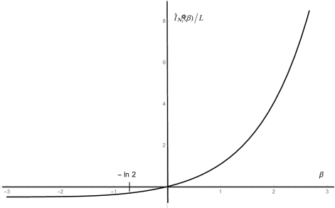
Figure 6: The bulk term of scaled cumulant generating function $\hat{I}_{\mathcal{N}_{t}^{\lozenge}}(\beta)/L$. Two functions are sewn at $\beta=-\ln 2$, so that the derivatives of all orders are continuous.

To obtain the values of the scaled cumulants, among which the first is the expected time average

$$c_{1}(\mathcal{N}_{t}^{\lozenge})=\lim_{t\to\infty}\mathbb{E}\frac{\mathcal{N}_{t}^{\lozenge}}{t}$$

and the second is the diffusion coefficient

$$c_{2}(\mathcal{N}_{t}^{\lozenge})=\lim_{t\to\infty}\frac{\mathbb{E}\left(\mathcal{N}_{t}^{\lozenge}\right)^{2}-\left(\mathbb{E}\mathcal{N}_{t}^{\lozenge}\right)^{2}}{t},$$

one needs to evaluate the derivatives of $\hat{I}_{\mathcal{N}_{t}^{\lozenge}}(\beta)$ at $\beta=0$. Technically nontrivial part is evaluating of derivatives of the function $Y(x)$ from (33) at $x=\pi/3$, which is summarized in A. Here we show the first four cumulants of $\mathcal{N}_{t}^{\lozenge}$, evaluated in two leading orders in $L$

$$c_{1}(\mathcal{N}_{t}^{\lozenge}) \simeq \frac{5}{8}L-\frac{3}{8}L^{-1},$$ (41)

$$c_{2}(\mathcal{N}_{t}^{\lozenge}) \simeq \left(\frac{9\sqrt{3}}{2\pi}-\frac{11}{6}\right)L+\left(\frac{3\sqrt{3}}{8\pi}-\frac{1}{2}\right)L^{-1},$$ (42)

$$c_{3}(\mathcal{N}_{t}^{\lozenge}) \simeq \left(\frac{217}{32}-\frac{243}{4\pi^{2}}\right)L+\frac{81}{16\pi^{2}}L^{-1},$$ (43)

$$c_{4}(\mathcal{N}_{t}^{\lozenge}) \simeq \left(\frac{719}{12}-\frac{1701\sqrt{3}}{10\pi}+\frac{162}{\pi^{2}}+\frac{324\sqrt{3}}{\pi^{3}}\right)L+\left(\frac{135\sqrt{3}}{8\pi^{3}}+\frac{27}{2\pi^{2}}-2\right)L^{-1}.$$ (44)

Let us now look at the associated rate function $I_{\mathcal{N}_{t}^{\lozenge}}(y)$. Since the scaled CGF is differentiable everywhere, the Gartner-Ellis theorem provides the rate function being its Legandre transform. It is defined parametrically by

$$I_{\mathcal{N}_{t}^{\lozenge}}(y) = \beta\hat{I}^{\prime}_{\mathcal{N}_{t}^{\lozenge}}(\beta)-\hat{I}_{\mathcal{N}_{t}^{\lozenge}}(\beta),$$ (45)

$$\phantom{I_{\mathcal{N}_{t}^{\lozenge}}(}y = \hat{I}^{\prime}_{\mathcal{N}_{t}^{\lozenge}}(\beta),$$ (46)

where $\beta\in\mathbb{R}$ is supposed to be eliminated between two expressions resulting in $I_{\mathcal{N}_{t}^{\lozenge}}(y)$ in the domain $y>0$, and $I_{\mathcal{N}_{t}^{\lozenge}}(y)=\infty$ for $y\leq 0$.

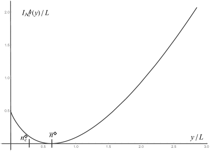
Figure 7: Rate function $I_{\mathcal{N}_{t}^{\lozenge}}(y)$.

It is clear that $\mathcal{N}_{t}^{\lozenge}/t$ and $I_{\mathcal{N}_{t}^{\lozenge}}(y)$ are extensive quantities, i.e. both are $O(L)$. Therefore, to rescale them to finite bulk values we consider $I_{\mathcal{N}_{t}^{\lozenge}}(y)/L$ as a function of $y/L$, both supposed to be finite as $L\to\infty$. The plot of this function is given in figure 7. Under this scaling the function $I_{\mathcal{N}_{t}^{\lozenge}}(y)/L$, has a single minimum at the point $y/L=\bar{n}^{\lozenge}=5/8$. The critical point corresponding to $\beta=-\ln 2$ is located at

$$y=\hat{I}^{\prime}_{\mathcal{N}_{t}^{\lozenge}}(-\ln 2):=Ln_{c}^{\lozenge},$$

where using the asymptotic form (63) of $Y(x)$ at $x\to 0$ we find

$$n_{c}^{\lozenge}\simeq\frac{4\ln 2-1}{6}\simeq 0.2954.$$

Like the scaled CGF the bulk part of the rate function is smooth everywhere, while the FSC abruptly change the order of magnitude from $O(L^{-1})$ to $O(e^{-L/\xi(\beta)})$.

Using the asymptotic forms (64,65) of $Y(x)$ and $\tilde{Y}(x)$ in the vicinity of $x=\pi/2$ and $x=\infty$, respectively, we obtain the rate function in extremal regimes of small and large values of $\mathcal{N}_{t}^{\lozenge}/t$.

$$\frac{I_{\mathcal{N}_{t}^{\lozenge}}(y)}{L} = \frac{y}{L}\left(\ln\left(\frac{y\pi}{2L}\right)-1\right)-\left(\frac{3}{4}+\frac{1}{\pi^{2}}\right)+O(L/y),\,\,\,y/L\to\infty,$$ (47)

$$\frac{I_{\mathcal{N}_{t}^{\lozenge}}(y)}{L} = \frac{1}{2}+\frac{y}{2L}\left(\ln\left(\frac{y}{2L}\right)-1\right)+O\left(\left(\frac{y}{L}\right)^{2}\right),\,\,\,y/L\to 0.$$ (48)

3.2.2 Large deviations of $\mathcal{N}_{t}^{\circlearrowleft}$

A similar set of data associated with the large deviations of $\mathcal{N}_{t}^{\circlearrowleft}$ is as follows. The leading order of the scaled CGF $\hat{I}{}_{\mathcal{N}_{t}^{\circlearrowleft}}(\alpha)=\Lambda_{0}(\alpha,0)$ is given by

$$\hat{I}{}_{\mathcal{N}_{t}^{\circlearrowleft}}(\alpha)=\frac{9\sqrt{3}}{4\pi L}\left(\left(\frac{\pi}{3}\right)^{2}-\left(\arccos\left[\frac{e^{\alpha/2}}{2}\right]\right)^{2}\right),$$ (49)

(see fig. 8). Therefore all the cumulants are of order of $L^{-1}.$

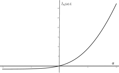
Figure 8: Scaled cumulant generating function of $\hat{I}{}_{\mathcal{N}_{t}^{\circlearrowleft}}(\beta)$

The first four cumulants are

$$c_{1}(\mathcal{N}_{t}^{\circlearrowleft}) \simeq \frac{3}{4}\frac{1}{L},$$ (50)

$$c_{2}(\mathcal{N}_{t}^{\circlearrowleft}) \simeq \left(\frac{1}{2}-\frac{3\sqrt{3}}{8\pi}\right)\frac{1}{L},$$ (51)

$$c_{3}(\mathcal{N}_{t}^{\circlearrowleft}) \simeq \left(\frac{1}{2}-\frac{3\sqrt{3}}{4\pi}\right)\frac{1}{L},$$ (52)

$$c_{4}(\mathcal{N}_{t}^{\circlearrowleft}) \simeq \left(\frac{5}{6}-\frac{3\sqrt{3}}{2\pi}\right)\frac{1}{L}.$$ (53)

The rate function $I_{\mathcal{N}_{t}^{\circlearrowleft}}(y)$ is again obtained from the scaled CGF as the Legendre transform. Its plot is given in fig. 9.

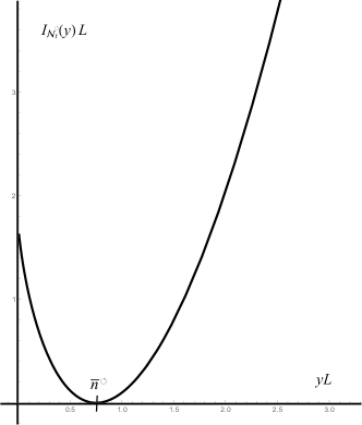
Figure 9: Rate function $I_{\mathcal{N}_{t}^{\circlearrowleft}}(y)$

It is defined parametrically via formulas similar to (45,46) up to change the subscript to $\mathcal{N}_{t}^{\circlearrowleft}$. It follows then that the magnitude of the rate function is of order of $I_{\mathcal{N}_{t}^{\circlearrowleft}}(y)=O(1/L)$, while expressions obtained are applicable in the limit $y\to 0,L\to\infty,yL=const$. Then $LI_{\mathcal{N}_{t}^{\circlearrowleft}}(y)$ is the finite function of $Ly$ that has a single minimum at $Ly=\bar{n}^{\circlearrowleft}=3/4$. The asymptotic behaviour of the $LI_{\mathcal{N}_{t}^{\circlearrowleft}}(y)$ corresponding to the limits $\alpha\to\pm\infty$.

$$I_{\mathcal{N}_{t}^{\circlearrowleft}}(y)L = \frac{5\pi\sqrt{3}}{16}+Ly\left(2\ln(Ly)-2+\ln\frac{2^{8}}{3^{5}}\right)+O((Ly)^{2}),yL\to 0$$

$$I_{\mathcal{N}_{t}^{\circlearrowleft}}(y)L = \frac{4\pi\left(Ly\right)^{2}}{9\sqrt{3}}-\frac{\sqrt{3}\pi}{4}+O(e^{-Ly}),\,\,\,yL\to\infty.$$

3.2.3 Mutual dependence of $\mathcal{N}_{t}^{\lozenge}$ and $\mathcal{N}_{t}^{\circlearrowleft}$

The simplest characteristics of mutual dependence of two random variables is the covariance. In our case this is the scaled covariance, the mixed scaled cumulant of the first degree in each variable,

$$c_{1,1}\left(\mathcal{N}_{t}^{\circlearrowleft},\mathcal{N}_{t}^{\lozenge}\right) = \lim_{t\to\infty}t^{-1}\left(\mathbb{E}\left(\mathcal{N}_{t}^{\circlearrowleft}\mathcal{N}_{t}^{\lozenge}\right)-\mathbb{E}\mathcal{N}_{t}^{\circlearrowleft}\mathbb{E}\mathcal{N}_{t}^{\lozenge}\right)$$

$$= \left.\frac{\partial^{2}\hat{I}_{\mathcal{N}_{t}^{\circlearrowleft},\mathcal{N}_{t}^{\lozenge}}(\alpha,\beta)}{\partial\alpha\partial\beta}\right|_{\alpha,\beta=0}.$$

Evaluating the derivatives of $\Lambda_{0}(\alpha,\beta)$ we obtain

$$Lc_{1,1}\left(\mathcal{N}_{t}^{\circlearrowleft},\mathcal{N}_{t}^{\lozenge}\right)=1-\frac{3\sqrt{3}}{8\pi}\simeq 0.793252.$$

The more detailed characteristics of mutual dependence that gives a meaning to the transition between the gapless and the gapped phases in the groundstate of the XXZ model is the conditional scaled CGF and conditional rate function. Specifically let us consider the scaled CGF of $\mathcal{N}_{t}^{\circlearrowleft}$ conditioned to the value of $\mathcal{N}_{t}^{\lozenge}$

$$\hat{I}_{\mathcal{N}_{t}^{\circlearrowleft}|\mathcal{N}_{t}^{\lozenge}}(\alpha|y)=\lim_{t\to\infty}t^{-1}\ln\mathbb{E}\left(e^{\alpha\mathcal{N}_{t}^{\circlearrowleft}}|\mathcal{N}_{t}^{\lozenge}=y\right).$$

Taking into account the form of the eigenvalue $\Lambda_{0}(\alpha,\beta)=\Lambda_{0}^{0}(\beta)+\Lambda_{0}^{1}(\alpha,\beta)$, where $\Lambda_{0}^{0}(\beta)=O(L)$ is the bulk part dependent only on $\beta$ and $\Lambda_{0}^{1}(\alpha,\beta)=o(L)$ is the FSC, we have

$$\hat{I}_{\mathcal{N}_{t}^{\circlearrowleft}|\mathcal{N}_{t}^{\lozenge}}(\alpha|y) \simeq \Lambda_{0}^{1}(\alpha,\beta(y))-\Lambda_{0}^{1}(0,\beta(y)),$$

where $\beta(y)$ is the solution of

$$y=\frac{\partial\Lambda_{0}^{0}(\beta)}{\partial\beta}.$$

The explicit formulas depend on the value of $y$. For $y/L\geq n_{c}^{\lozenge}$ that corresponds to $\beta(y)>-\ln 2$ we have the conditioned scaled CGF, which coincides with the unconditioned one (49) up to an overall $y$-dependent factor

$$\hat{I}_{\mathcal{N}_{t}^{\circlearrowleft}|\mathcal{N}_{t}^{\lozenge}}(\alpha|y)=\frac{g(\beta(y))}{L}\left(\left(\frac{\pi}{3}\right)^{2}-\left(\arccos\left[\frac{e^{\alpha/2}}{2}\right]\right)^{2}\right).$$

Here

$$g(\beta)=\frac{\pi\sqrt{4e^{2\beta}-1}}{2\arccos\frac{e^{-\beta}}{2}\left(\pi-\arccos\frac{e^{-\beta}}{2}\right)},$$

$\beta(y)$ solves the equation

$$y/L=\frac{d}{d\beta}\left(\left(e^{\beta}-\frac{1}{4}e^{-\beta}\right)\,Y\left[\arccos(e^{-\beta}/2)\right]\right),$$

and we imply that $y=O(L)$.

For $y/L<n_{c}^{\lozenge}$ we obtain purely exponential function of $\alpha$ scaled by the $y$-dependent factor that decays exponentially as $L$ grows to infinity.

$$\hat{I}_{\mathcal{N}_{t}^{\circlearrowleft}|\mathcal{N}_{t}^{\lozenge}}(\alpha|y)=\left(e^{\alpha/2}-1\right)a(\beta(y))e^{-L/\xi(\beta(y))}L^{-1/2}.$$

Here, $\beta(y)$ solves the equation

$$y/L=\frac{d}{d\beta}\left(\left(\frac{1}{4}e^{-\beta}-e^{\beta}\right)\,\tilde{Y}\left[\mathrm{arccosh}(e^{-\beta}/2)\right]-1\right)$$

and the functions $a(\beta),\xi(\beta)$ are those appeared in (3.2.1).

Thus, up to the overall scale factor, which can be incorporated into the time scale, the scaled CGF of $\mathcal{N}_{t}^{\circlearrowleft}$ conditioned to a value of $\mathcal{N}_{t}^{\lozenge}$ has two different functional forms depending on whether the $\mathcal{N}_{t}^{\lozenge}/(Lt$) is greater or less than $n_{c}^{\lozenge}$. This sharp change of behaviour at the critical point can be made continuous upon looking at it in the smaller scale. The scaling regime of the groundstate of the XXZ Hamiltonian mentioned in the end of subsection 3.1 suggests that if we consider the scaling

$$y/L=n_{c}^{\lozenge}-\frac{s}{\log L}$$

with $s>0$, the conditional scaled CGF will take the form

$$\hat{I}_{\mathcal{N}_{t}^{\circlearrowleft}|\mathcal{N}_{t}^{\lozenge}}(\alpha|y)=L^{-1}f(s,\alpha),$$

where $f(s,\alpha)$ is a crossover function related to $h(x,\varphi)$ from (38) by a suitable variable change. The two functions obtained above are expected to be restored as limiting cases of $f(s,\alpha)$ in the limits $s\to 0$ and $s\to\infty.$ An explicit form of this function is yet to be determined.

4 Discussion and conclusion.

To summarize, we obtained the large deviation functions for two additive functionals on the trajectories of RPM: the total number of tiles removed by avalanches $\mathcal{N}_{t}^{\lozenge}$ and the total number of global avalanches $\mathcal{N}_{t}^{\circlearrowleft}.$ Technically, all the properties of the large deviations described stem from the corresponding properties of the groundstate of twisted XXZ Hamiltonian. What we would like to do here is to provide them with a stochastic interpretation.

First, we focused on the expressions of the scaled CGM $\hat{I}_{\mathcal{N}_{t}^{\lozenge}}(\beta)$ and $\hat{I}_{\mathcal{N}_{t}^{\circlearrowleft}}(\alpha)$ separately and on the corresponding rate functions $I_{\mathcal{N}_{t}^{\lozenge}}(x),I_{\mathcal{N}_{t}^{\circlearrowleft}}(y)$ in the limit $L\to\infty$. The first outcome of these results are the asymptotics of the scaled cumulants of $\mathcal{N}_{t}^{\lozenge}$ in two leading orders and of $\mathcal{N}_{t}^{\circlearrowleft}$ in the leading order in $L$. The cumulants of the first order, the means, can be also obtained from an averaging over the stationary state. The asymptotic formulas (41,50) obtained indeed reproduce the large $L$ expansions of the conjectured exact formulas (21,22) respectively. The cumulants of higher orders involve unequal time correlations. Thus, they are beyond the scope of the stationary state analysis and to our knowledge are presented for the first time. To find exact expression of the cumulants at arbitrary finite $L$ one can try the technique of perturbative solution of T-Q relations which was successfully applied to the asymmetric simple exclusion process in [33]. The case of RPM however seems even more challenging because of nontrivial structure of the groundstate solution of Bethe equations even at the stochastic point.

Our analysis also explains the observation made in [34] of the spin current in the XXZ chain with twist $\varphi=-2\pi/3$ being related to the particle current in nonlocal asymmetric simple exclusion process (NASEP) via the factor $\sqrt{3}$. The NASEP was proposed in [34] as a model obtained from RPM by the usual interface-particle system correspondence. Specifically, the upper boundary of a stable configuration in the periodic Dyck path representation is associated to an $L/2$-particle configuration on a one-dimensional lattice consisting of $L$ sites. A down-step of the line going from horizontal position $i$ to $i+1$ is mapped to the site $i$ of the 1D lattice occupied by a particle and the up-step is mapped to an empty site. The time evolution of the RPM is also naturally mapped to the evolution of the particle system.

In particular, the NASEP current per bond is defined in [34] as the number of right jumps minus the number of left jumps of particles crossing a bond per unit time. Alternatively one can think of the total distance traveled by particles, i.e. difference of numbers of right and left jumps on the whole lattice, divided by $L$. Every adsorption of a tile in a local minimum (valley) contribute $+1$ and the avalanche of size $n$ contribute $-(n-1)$ into the into the distance. Here, minus one corresponds to the extra tile starting the avalanche that was included into the avalanche size and does not contribute to the distance traveled by particles in NASEP. The global avalanches do not contribute to the current according to definition of [34]. As the number of adsorbed tiles should be approximately (up to a bounded difference) equal to the number of tiles removed by both local and global avalanches, the total distance traveled by all the particles in NASEP approximately equals $-\mathcal{N}_{t}^{\circlearrowleft}$. Thus, up to the sign the mean current $J$ in NASEP coincides with $c_{1}(\mathcal{N}_{t}^{\circlearrowleft})$.

At the same time the spin current in $XXZ$ model defined as $J^{z}=\left\langle 0\left|J_{i}^{z}\right|0\right\rangle,$ where $J_{i}^{z}=\mathrm{i}(\sigma_{i}^{+}\sigma_{i+1}^{-}-\sigma_{i}^{-}\sigma_{i+1}^{+})$ and the averaging is over the groundstate of the XXZ Hamiltonian, can be evaluated as $J^{z}\simeq-\partial E_{L}^{XXZ}(\Delta,e^{\mathrm{i}\varphi/L})/\partial\varphi$ in the leading order in $L$. Going from the differentiation of the XXZ energy in the twist variable $\varphi$ to that of the eigenvalue of the stochastic generator $\mathcal{L}_{(\alpha,\beta)}$ in the variable $\beta$ we obtain the desired relation.

Let us discuss the large deviation functions beyond the cumulants. The quantity $\mathcal{N}_{t}^{\lozenge}$ grows by elementary random increments $\mathcal{\delta N}_{\tau}^{\lozenge}(x)$ associated with space-time positions in $\left\{(x,\tau)\in(1,\dots,L)\times[0,t]\right\}$. The total rate of growth is of order of $L$, which suggests that the main part of the scaled CGF $\hat{I}_{\mathcal{N}_{t}^{\lozenge}}(x)$ scales linearly with $L$ and, hence, the usual CGF of $\mathcal{N}_{t}^{\lozenge}$ is linear in $Lt$. If the increments were uncorrelated, the CGF would be purely linear. The spacial correlations lead to appearance of FSC to the scaled CGF.

Usually, the FSC to the bulk free energy in equilibrium systems come from the geometric factors like surface, edges, corners e.t.c., each contribution being scaled as an integer power of system size according to its dimension. These contributions, however, are not present in the systems with periodic boundary conditions [35]. In such systems away from criticality, which are characterized by a finite correlation length, the FSC are exponentially small. In critical systems with infinite correlation length there is also the fluctuation induced Casimir-like term that decays as a power of system size [35]. Thinking about CGM as an analogue of the free energy one can expect similar scenario in the non-equilibrium setting. Our analysis of $\hat{I}_{\mathcal{N}_{t}^{\lozenge}}(\beta)$ reveals the transition from critical phase, $\beta>-\log 2$, with the FSC of order of $O(1/L)$ to the noncritical phase, $\beta<-\log 2$, where the FSC decay exponentially.

In particular the system is critical at $\beta=0$. An indication of the infinite correlation length is the presence of global avalanches, which happen with the frequency of order of inverse system size. The probability distribution of the number of global avalanches per unit time behaves as

$$\mathbb{P}\left(\frac{\mathcal{N}_{t}^{\circlearrowleft}}{t/L}\approx x\right)\asymp\exp\left(-\frac{t}{L}I(x)\right),$$ (54)

where we used the notation $I(x)=LI_{\mathcal{N}_{t}^{\circlearrowleft}}(x)$ to remove the $L$-dependence from the rate function and to emphasize that the effective time units scale linearly with system size. This time scaling suggests the dynamical exponent to be $z=1$, which is the usual companion for conformal invariance. The universality of global avalanche statistics over the critical phase and the phase transition to the non-critical phase are most clearly manifested with the rate function for $\mathcal{N}_{t}^{\circlearrowleft}$ conditioned to a given value of $\mathcal{N}_{t}^{\lozenge}/t=yL.$ To this end, it is convenient to introduce the effective unit of time $\tau(y)$ being the coefficient of $\hat{I}_{\mathcal{N}_{t}^{\circlearrowleft}|\mathcal{N}_{t}^{\lozenge}}(\alpha|y)$ encapsulating all the dependence on $y$. $\tau(y)$ scales linearly with $L$, $\tau(y)=O(L)$, in the critical phase $y>n_{c}^{\lozenge}$ and grows exponentially, $\tau(y)=O(e^{L/\xi(\beta(y))}\sqrt{L})$ otherwise, i.e. $0<y<n_{c}^{\lozenge}$. Then the conditioned probability can be given in a universal form

$$\mathbb{P}\left(\left.\frac{\mathcal{N}_{t}^{\circlearrowleft}}{(t/\tau(y))}\approx x\right|\frac{\mathcal{N}_{t}^{\lozenge}}{t}=yL\right)\asymp\exp\left(-\frac{t}{\tau(y)}I(x)\right),$$

where $I(x)$ is the same as in (54) over the whole critical phase and changes to

$$I(x)=2x(\log 2x-1)+1$$

in the non-critical one. The latter is nothing but the rate function of the Poisson distribution, which suggests the global avalanches being independent events, i.e. they happen so rare in the non-critical regime that the system forgets the past from one global avalanche to another.

We also explicitly obtained the tails of the rate functions. Sometimes from the tails one can get an idea how the system should be modified to fall into an extremal regime. In particular we found that $I_{\mathcal{N}_{t}^{\lozenge}}(y)\to 1/2$ as $y\to 0$, which means that the probability of trajectories keeping $\mathcal{N}_{t}^{\lozenge}$ small behaves as $\exp\left(-Lt/2\right)$. We interpret this regime as the system remaining in the substrate configuration by forbidding for the tiles to arrive anywhere except the peaks, i.e. at $L/2$ sites. The rate functions $I_{\mathcal{N}_{t}^{\circlearrowleft}}(x)$ also tends to a constant as $x\to 0.$ As $x\to\infty$ the functions $I_{\mathcal{N}_{t}^{\lozenge}}(x)$ and $I_{\mathcal{N}_{t}^{\circlearrowleft}}(x)$ behave in Poissonian-like and Gaussian-like manner respectively. The interpretation of the three latter regimes is yet to be found. In general detailed studies of the stochastic processes conditioned to atypical fluctuations requires studies of the maximal eigenvector of the stochastic generator rather than the eigenvalue. This is the subject for further work.

As another unsolved problems we leave the construction of the crossover function, which would connect the regimes $\mathcal{N}_{t}^{\lozenge}/t>n_{c}^{\lozenge}L$ and $\mathcal{N}_{t}^{\lozenge}/t<n_{c}^{\lozenge}L$ of the conditional rate function $I_{\mathcal{N}_{t}^{\circlearrowleft}|\mathcal{N}_{t}^{\lozenge}}(\alpha|y)$.

Appendix A Particular values and asymptotics of $Y(x)$ and $\tilde{Y}(x)$.

Here we present the result of explicit evaluation of integral (33) in $Y(x)$ and its derivatives at points $x=\pi/3,0,\pi/2$. It can be done using the residue calculus by closing the contour of integration through the upper (lower) half-planes. This becomes possible after introducing a suppressing factor $e^{i\epsilon x}(e^{-i\epsilon x})$ with small $\epsilon>0$ into the integrand and sending $\epsilon$ to zero in the end. The values of derivatives of $Y^{(n)}(\pi/3)$ are listed below up to $n=6$.

$$Y\left(\frac{\pi}{3}\right) = \frac{4}{3},$$ (55)

$$Y^{\prime}\left(\frac{\pi}{3}\right) = -\frac{25}{6\sqrt{3}},$$ (56)

$$Y^{{}^{\prime\prime}}\left(\frac{\pi}{3}\right) = \frac{18\sqrt{3}}{\pi}-3,$$ (57)

$$Y^{(3)}\left(\frac{\pi}{3}\right) = \frac{463}{8\sqrt{3}}-\frac{54}{\pi}-\frac{243\sqrt{3}}{\pi^{2}},$$ (58)

$$Y^{(4)}\left(\frac{\pi}{3}\right) = \frac{15059}{18}-\frac{9306\sqrt{3}}{5\pi}+\frac{972}{\pi^{2}}+\frac{3888\sqrt{3}}{\pi^{3}},$$ (59)

$$Y^{(5)}\left(\frac{\pi}{3}\right) = -\frac{33185\sqrt{3}}{4}+\frac{8946}{\pi}+\frac{72495\sqrt{3}}{\pi^{2}}-\frac{19440}{\pi^{3}}-\frac{72900\sqrt{3}}{\pi^{4}},$$ (60)

$$Y^{(6)}\left(\frac{\pi}{3}\right) = -\frac{3938533}{6}+\frac{10658034\sqrt{3}}{7\pi}-\frac{425250}{\pi^{2}}-\frac{2658420\sqrt{3}}{\pi^{3}},$$ (62)

$$+\frac{437400}{\pi^{4}}+\frac{1574640\sqrt{3}}{\pi^{5}}.$$

The expansion around $x=0$ and $x=\pi/2$ yields

$$Y(x) = \frac{2\ln 2}{x^{2}}+\frac{\ln 2}{3}-\frac{1}{6}+O(x)\text{,\,\,}x\to 0,$$ (63)

$$Y\left(\frac{\pi}{2}+x\right) = \frac{2}{\pi}-\left(\frac{1}{2}+\frac{2}{\pi^{2}}\right)x+\frac{24+17\pi^{2}}{9\pi^{3}}x^{2}+O(x^{3}),\,\,\,x\to 0.$$ (64)

Finally we provide the expansion of the sum in (36)

$$\tilde{Y}(x)=2e^{-x}+10e^{-3x}+10e^{-5x}+O(e^{-7x}),\,\,\,x\to\infty.$$ (65)

References

- [1] Cramèr H, 1938 Sur un nouveau théorème-limite de la théorie des probabilités. Actualités Scientifiques et Industrialles 736 5-23. Colloque Consecré à la Théorie des Probabilités 3. Hermann, Paris.
- [2] Wentzell A D and Freidlin M I, 1970 Russ. Math. Surv., 25, 1
- [3] Donsker M D and Varadhan S R S, 1975 Comm. Pure Appl. Math. 28 1.
- [4] Donsker M D and Varadhan S R S, 1975 Comm. Pure Appl. Math. 28 279
- [5] Donsker M D and Varadhan S R S, 1976 Comm. Pure Appl. Math. 29 389
- [6] Derrida B, 2007 J. Stat. Mech. P07023
- [7] Derrida B and Lebowitz J L, 1998 Phys. Rev. Lett. 80 209
- [8] Appert-Rolland C, Derrida B, Lecomte V and Van Wijland F, 2008 Phys. Rev. E 78 021122
- [9] Edwards S F and Wilkinson D R, 1982 In Proc. R. Soc. Lond. A 381 17
- [10] Kardar M, Parisi G and Zhang Y-C, 1986 Phys. Rev. Lett. 56 889.
- [11] De Gier J, Nienhuis B, Pearce P A and Rittenberg V, 2004 J. Stat. Phys. 114 1
- [12] Alcaraz F C and Rittenberg V, 2007 J. Stat. Mech. P07009.
- [13] De Gier J, 2005 Discr. Math. 298 365
- [14] Alcaraz F C and Rittenberg V, 2015 J. Stat. Mech. P11012
- [15] Levy D, 1991 Phys. Rev. Lett. 67 1971
- [16] Alcaraz F C, Barber M N and Batchelor M T, 1988 Ann. Phys. Mar 1;182(2):280-343.
- [17] Razumov A V and Stroganov Yu G, 2001 J. Phys. A: Math. Gen. 34 3185
- [18] Batchelor MT, De Gier J and Nienhuis B, 2001 J. Phys. A: Math. Gen. 34 L265
- [19] Razumov A V and Stroganov Yu G, 2004 Theor. Math. Phys. 138 333
- [20] Razumov A V and Stroganov Yu G, 2005 Theor. Math. Phys. 142 237
- [21] Mitra S, Nienhuis B, De Gier J and Batchelor M T, 2004 J. Stat. Mech. P09010.
- [22] Pyatov P, 2004 J.Stat.Mech. P09003
- [23] Yang C N and Yang C P, 1966 Phys. Rev. 150 321
- [24] Yang CN andYang C P, 1966 Phys. Rev. 150 327.
- [25] De Vega H J and Woynarovich F, 1985 Nucl. Phys. B 251 439
- [26] Hamer C J, 1985 J. Phys. A: Math. and Gen. 18 L1133
- [27] Barber M N and Batchelor M T, 1990 Int. J. Mod. Phys. B 05 953
- [28] Hamer C J, Quispel G R and Batchelor M T, 1987 J. Phys. A: Math. Gen. 20 5677.
- [29] Destri C and De Vega HJ, 1989 Phys. Lett. B. 223 365
- [30] Hamer C J, 1986 J. Phys. A: Math. Gen. 19 3335
- [31] Virosztek A and Woynarovich F, 1984 J. Phys. A: Math. and Gen. 17 3029.
- [32] des Cloiseaux J and Gaudin M, 1966 J. Math. Phys. 7 1384
- [33] Prolhac S and Mallick K J Phys A: Math and Theor 41.17 (2008): 175002.
- [34] Alcaraz F C and Rittenberg V, 2013 J. Stat. Mech. P09010
- [35] Fisher M E and Barber M N, 1972 Phys. Rev. Lett. 28 1516.