Function approximation using gradient information with application to parametric and stochastic differential equations

Abstract

In the paper we consider the problem of multivariate function approximation in polynomial basis. In order to solve this problem, we adjust the least squares method (LSM) by adding information about derivatives of the function. This modification allows reducing the number of evaluations of approximating function while keeping the accuracy at the appropriate level. We propose several techniques for time-efficient calculation of derivatives in various applications. Numerical examples are given for comparison between the standard LSM and the proposed approach.

65D05, 65D15, 41A10, 35C11

1 Introduction

Multivariate function approximation is a complex problem that arises in many practical applications. We consider the situation when the cost of a function calculation in a point is rather high (see [32, 33] where polynomial approximation is applied to electric circuit). One of the standard approaches to the approximation is using linear combination of elements from some polynomial basis as an approximant and the least squares method (LSM) to find the coefficients. To reduce the complexity and to improve the accuracy of the approximation it is needed to solve two problems, how to decrease the number of sample points and how to appropriately choose them.

In our approach, the first problem is solved by calculation of the function gradient. The classical result by Baur and Strassen [8] on automatic differentiation states that if the function is given as a composition of elementary operations (i.e. it is a rational function), then the gradient can be computed at most $4N$ operations, where $N$ is the cost of a single evaluation of the function. The method of computing derivatives is also known as “backpropagation”. This method allows fast calculating the gradient of the function that also consists of elementary functions and user-defined ones [20]. In our research we use Python package autograd [2] since it allows calculating derivatives in an efficient and convenient way. However, in a case when the function is given as a black box, it is hard to find its derivatives with autograd. In order to accelerate the calculation of derivatives in such cases, we use ad hoc methods. These methods also enable calculating function in less number of points compared to the standard ones while keeping high accuracy.

The second problem of sampling can be solved in several ways. We use the algorithm based on maximum volume concept [26, 5] in high-dimensional problems. Additionally we use Latin Hypercube Sampling (LHS) (see [25]). Monte-Carlo method was used as a reference.

Main contributions of the paper are

• we propose a new method of multivariate function approximation with the use of its derivatives;

• numerical experiments that demonstrate the excellence in the accuracy of the proposed approach over the standard one in a number of cases are conducted;

• we propose several techniques for accelerated calculation of derivatives so it can be reached the equivalent accuracy in much less time when the cost of function evaluation is high.

2 Mathematical background

2.1 System matrix

Consider the problem of a multivariate polynomial approximation of a smooth function $f(x)$, $x=(x^{(1)},\,x^{(2)},\,\ldots,\,x^{(l)})\in\mathbb{R}^{l}$. One of the classical approaches is to use the linear combination of some linearly independent polynomials $\{P_{i}\}$

(1) $$f(x)\approx\widehat{f}(x)=\sum_{i=1}^{M}\alpha_{i}P_{i}(x).$$

Unknown coefficients $\alpha_{i}$ in (1) can be found using the least squares method (LSM) which minimize the $l_{2}$ norm of the residual in some selected set of points $G=\{\xi_{1},\,\xi_{2},\,\ldots,\,\xi_{m}\}\subset\mathbb{R}^{l}$, $m\geq M$

$$\sum_{i=1}^{m}\left(f(\xi_{i})-\widehat{f}(\xi_{i})\right)^{2}\to\min_{\{\alpha_{i}\}}.$$

Let the values of the function $f$ and its gradient be known at the points of the set $G$. We use these values and the LSM approach to solve the following problem

(2) $$A\alpha=F,$$

where the vector $\alpha=\{\alpha_{1},\,\alpha_{2},\,\ldots,\,\alpha_{m}\}$ is the vector of unknown coefficients of decomposition (1); $F\in\mathbb{R}^{(l+1)m}$ is the vector of values of the function $f$ and its gradient at the points of the set $G$

(3) $$F_{i}=\left\{\begin{aligned} f(\xi_{i})&,&\;\;0<i&\leq m,\\ \partial_{1}f(\xi_{i\operatorname{{}mod}m})&,&m<i&\leq 2m\\ \partial_{2}f(\xi_{i\operatorname{{}mod}m})&,&2m<i&\leq 3m\\ \cdots\\ \partial_{l}f(\xi_{i\operatorname{{}mod}m})&,&lm<i&\leq(l+1)m,\end{aligned}\right.$$

here $\partial_{i}$ is $i^{\text{th}}$ gradient’s component

$$\partial_{i}:=\frac{\partial}{\partial x^{(i)}}.$$

The matrix $A=\{a_{ij}\}$ has the following elements

(4) $$a_{ij}=\left\{\begin{aligned} P_{j}(\xi_{i})&,&\;\;0<i&\leq m,\\ \partial_{1}P_{j}(\xi_{i\operatorname{{}mod}m})&,&m<i&\leq 2m\\ \partial_{2}P_{j}(\xi_{i\operatorname{{}mod}m})&,&2m<i&\leq 3m\\ \cdots\\ \partial_{l}P_{j}(\xi_{i\operatorname{{}mod}m})&,&lm<i&\leq(l+1)m\end{aligned}\right..$$

In this approach we use additional information about the function (derivatives). Thus the resulting matrix has more rows than without using derivatives. So we expect that adding a new column to the system matrix does not change its full-column rank property. That means that we can use polynomials of a higher degree to increase the accuracy of the approximation.

As a set of polynomials $\{P_{i}\}$ we take a subset of the tensor product of unidimensional polynomials $f_{i}$ of the form

$$f_{\beta_{1}}(x^{(1)})f_{\beta_{2}}(x^{(2)})\cdots f_{\beta_{l}}(x^{(l)})$$

with hyperbolic transaction scheme (see review [18]) where polynomials degree $\{\beta_{i}\}$ satisfy inequality

$$\sum_{i=1}^{l}\beta_{i}^{p}\leq q^{p},\qquad\beta_{i}\in\mathbb{N}\cup\{0\},$$

for some $p\in(0,1]$. In the case $p=1$, total number of elements of the polynomial set is equal to $(l+p)!/(l!p!)$.

3 Algorithm of multivariate function approximation using derivatives

We propose the following algorithm for the method of function approximation with the use of function derivatives based on the ideas described in Sec. 2.

Algorithm 1 Algorithm for function approximation using the information of its derivatives

0:  Number of points $m$, function evaluator, function derivatives evaluator, function domain

0:  Coefficients of the expansion $\alpha$

1:  Select $N\geq m$ nodes $\{\xi_{1},\,\xi_{2},\,\ldots,\,\xi_{N}\}$ from the function domain using one of the classical algorithms

2:  If $N>m$, use maxvol algorithm to reduce the number of the selected points to $m$ and select some subset of the set from the first step

3:  Compute right-hand side $F$ using (3)

4:  Form the system matrix $A$ using (4)

5:  Solve the least squares problem $\alpha=A^{+}F$

At the first step of the approximation of the given function $f$ we choose the points where the function is evaluated. We use random sampling, uniform distribution, Latin Hypercube Sampling (LHS) in different experiments. In some cases we reduce the number of selected points using maxvol [5] procedure.

Then we form a vector of the right-hand side of the overdetermined system (2) by calculating function values and its derivatives at the selected points. The choice of a method that we used for derivative calculation depends on the task. Different approaches are described below in Sec. 5–6.

The resulting coefficients $\alpha$ can be used to evaluate the values of the function approximant directly. They can also be used to find some properties of the unknown function such as the mean value and standard deviation if the function is random one as in the example in Sec. 5.3.2.

The complexity of the algorithm depends on the complexity of function and calculation of its derivatives. We assume that an asymptotic complexity of derivatives calculation is the same as the function calculation one, i.e. the function satisfies the Baur and Strassen theorem [8]. Theoretically we need no more then $4N$ operations to find all derivatives if the function is rational one, where $N$ is the number of operations necessary to find the function. Several effective ways for fast computation of the derivatives are given below in the following sections. If the function evaluation at one point takes a long time, our approach allows to dramatically decrease the total calculation time in the case of high-dimensional tasks ($d\gg 4$) to get the same size of the system matrix $A$. We do not know the exact estimates for the Lebesgue constant for our approach, so we can not theoretically estimate the accuracy of the approximation.

Now we demonstrate the quality of the proposed approach on model examples.

4 Model example of approximation

We consider the following function of two variables

$$f(x_{1},\,x_{2})=\exp\left(-x_{1}^{2}-0.5(x_{2}-1)x_{2}\right)$$

to check interpolation error with and without using the information of its derivatives.

The interpolation is performed on the rectangle $[-2,\,2]^{2}$. We use different number of points $N=50$, $200$ where the function values and its gradient are calculated. We use maxvol algorithm to select the desired amount of points from the initial set of $10^{4}$ points uniformly distributed on the rectangle. Chebyshev polynomials are used as the basis functions.

Results are shown in Fig. 1–2, where $L_{2}$, relative error of the interpolation, is given as a function of the number of the monomials.

(a) Number of points is $N=50$

(b) Number of points is $N=200$

Figure 1: Error of interpolation without noise

(a) Number of points is $N=50$

(b) Number of points is $N=200$

Figure 2: Error of interpolation with noise

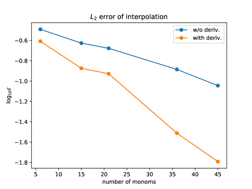
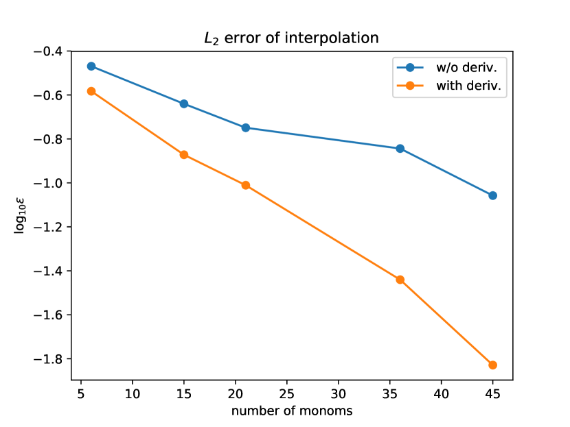
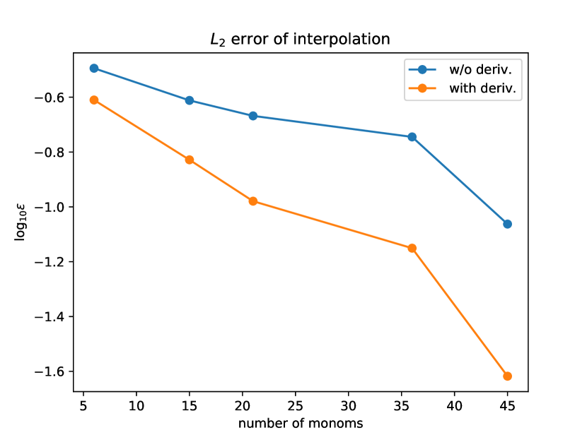
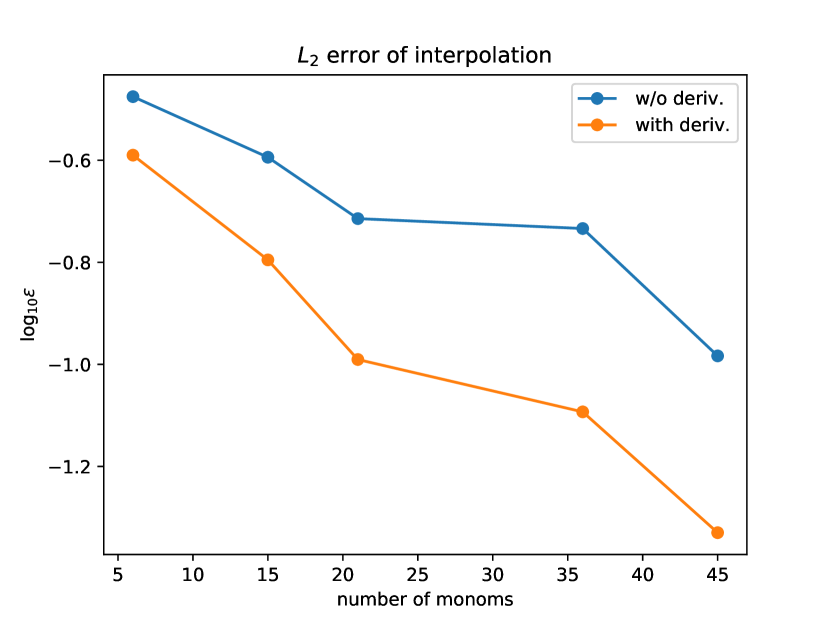
One can see that the derivative approach gives more accurate results.

Now we will show how this approach can be applied to parametric ODEs.

5 Parametric Ordinary Differential Equations

5.1 Mathematical statement

Consider a linear differential algebraic equation (DAE) with coefficients depending on $l$ parameters $\vec{\xi}=[\xi_{1},\,\xi_{2},\,\ldots,\,\xi_{l}]$

(5) $$E(\vec{\xi})\frac{d\vec{x}(t,\vec{\xi})}{dt}+A(\vec{\xi})\vec{x}(t,\vec{\xi})=B\vec{u}(t).$$

Here $E$ and $A$ are $n\times n$ matrices, $\vec{x}(t,\vec{\xi})\in\mathbb{R}^{n}$ is the vector of unknowns, $\operatorname{rank}E\leq n$, $\operatorname{rank}A=n$. The matrix $B$ is $n\times d$, $\vec{u}(t)\in\mathbb{R}^{d}$ is the vector of inputs. This kind of equations describes, for example, electric circuits which contain only linear elements. In the case of circuits with non-linear elements, we first linearise it on each time step and still get (5) where matrices will be time-dependent.

As an example some input parameters of the equation (5) can be random values. The problem is to find the distribution of the solution. Physically it means that some circuit parameters are not known exactly because of the nature of the environment, and we want to know some properties of the output signal. See [32] for examples of the polynomial chaos approach to several electric schemes. Now we will show how to obtain the derivatives of the solution $\vec{x}$ efficiently.

5.2 Obtaining derivatives

5.2.1 Derivatives via new right-hand side of the same equation

Differentiating the equation (5) with respect to the $i^{\text{th}}$ parameter yields

(6) $$E(\vec{\xi})\frac{d\vec{x}_{i}(t,\vec{\xi})}{dt}+A(\vec{\xi})\vec{x}_{i}(t,\vec{\xi})=B_{i}\vec{u}(t)-E_{i}(\vec{\xi})\frac{d\vec{x}(t,\vec{\xi})}{dt}-A_{i}(\vec{\xi})\vec{x}(t,\vec{\xi}),$$

where

$$\mathcal{X}_{i}:=\frac{\partial}{\partial\xi_{i}}\mathcal{X}\;\text{ for }\;\mathcal{X}=x(t,\vec{\xi}),E(\vec{\xi}),A(\vec{\xi}),B(\vec{\xi}).$$

So, if we have solved the equation (5), then we can solve (6) with a known right-hand side to obtain the derivative with respect to the parameters.

5.2.2 Derivatives via solving the extended system

Consider the following equation

(7) $$\widetilde{E}(\vec{\xi})\frac{d\vec{x}(t,\vec{\xi})}{dt}+\widetilde{A}(\vec{\xi})\widetilde{\vec{x}}(t,\vec{\xi})=\widetilde{B}u(t),$$

with matrices

(8) $$\widetilde{E}=\begin{pmatrix}E&0&0&\dots&0\\ E_{1}&E&0&\dots&0\\ E_{2}&0&E&\dots&0\\ {5}\\ E_{l}&0&0&\dots&E\end{pmatrix},\quad\widetilde{A}=\begin{pmatrix}A&0&0&\dots&0\\ A_{1}&A&0&\dots&0\\ A_{2}&0&A&\dots&0\\ {5}\\ A_{l}&0&0&\dots&A\end{pmatrix},\quad\widetilde{B}=\begin{pmatrix}B\\ 0\\ 0\\ \cdots\\ 0\\ \end{pmatrix}.$$

Then the solution of this equation will be the vector

$$\widetilde{\vec{x}}=\{\vec{x};\,\vec{x}_{1};\,\vec{x}_{2};\,\ldots;\,\vec{x}_{l}\}.$$

We can easily obtain the LU factorization of the matrix with such a block structure as in (8). Indeed, denote the LU factorization of the block $A$ as $A=LU$. Then $\widetilde{A}=\widetilde{L}\widetilde{U}$ and

(9) $$\widetilde{U}=\begin{pmatrix}U&0&0&\dots&0\\ 0&U&0&\dots&0\\ 0&0&U&\dots&0\\ {5}\\ 0&0&0&\dots&U\end{pmatrix},\quad\widetilde{L}=\begin{pmatrix}L&0&0&\dots&0\\ L_{1}&0&0&\dots&0\\ L_{2}&0&0&\dots&0\\ {5}\\ L_{l}&0&0&\dots&0\end{pmatrix},$$

where matrices $L_{i}$ for $i=1,\dots,l$ are such that

$$A_{i}=L_{i}U,\quad i=1,\dots,l.$$

and they can be calculated fast since $U$ is an upper triangular matrix and each $A_{i}$ is sparse.

Let the matrix $A$ be of size $n\times n$, number of operations required for solving system with the matrix $\widetilde{A}$ is

(10) $$N=O(n^{3})+O(c_{1}n^{2})+O(ln^{2})+O(c_{2}).$$

Here $c_{1}$ is the total number of non-zero rows in the matrices $A_{i}$, $c_{2}$ is the total number of non-zeros elements in matrices $A_{i}$. The first two terms in (10) correspond to the LU-decomposition of the matrix $\widetilde{A}$, the last two terms are the number of operations required for the solution step.

5.3 Some numerical examples

In this section we present several examples of fast calculation of the function derivatives using the approaches described above. Their timings are given as well as the asymptotic complexity.

5.3.1 Linear electrical scheme

Consider the linear scheme in Fig. 3 as an example.

Figure 3: Testing scheme.

The electrical schemes that we use in the experiments consists of $967$ and $7687$ resistors, only central part of the scheme is shown in Fig. 3. The closest elements to the inputs points are treated as unknown parameters in the sense that we take derivatives with respect to them. For example, the first ten elements are listed below

$$R_{35-36},\,R_{27-35},\,R_{28-36},\,R_{35-43},\,R_{36-44},$$

$$R_{27-28},\,R_{34-35},\,R_{36-37},\,R_{43-44},\,R_{26-27}.$$

Number of parameters $l$	5	8	12	300	600
Time (sec.)	0.07	0.11	0.16	3.96	8.18

Table 1: Built-in sparse LU-solver timings

Number of parameters $l$	2	10	300	600
Time (sec. $\times 10^{8}$) for number of elements $k=967$	0.40	0.47	1.41	2.07
Time (sec. $\times 10^{10}$) for number of elements $k=7687$	1.99	2.01	2.66	3.30

Table 2: Autograd timings

The timings of solving the equation (7) with a different number of unknown parameters are shown in Table 1. Matrices were stored in Compressed Sparse Row (CSR) format, and the solution was obtained with Python build-in LU-factorization. We can see that the times grows almost linear in the number of the parameters when the block structure of the matrices is not accounted. The number of operations for the solution of the system with the LU-decomposition (9) of the matrix $\widehat{A}$ for the electric circuit in Fig. 3 is shown in Table 3.

Number of parameters $l$	2	10	300	600
Time (sec.)	1415	1437	1366	1332

Table 3: Timings for sparse system matrix solving

We used the scheme with $647$ elements to measure the time in the case of calculating derivatives using autograd. The timings are shown in Table 2. We can see that the timings are practically independent of the number of arguments.

5.3.2 Non-liner electrical scheme with noise

We can apply our approach to model schemes that also have non-linear elements. Consider a common-source amplifier shown in Fig. 4.

Figure 4: Common-source amplifier

We use the MOSFET model of transistor in our numerical simulation. Python package ahkab [1] was used for this purpose. In the scheme 4 the input voltage $V_{\text{in}}$ is constant, and the voltage $V_{\text{dd}}$ is equal to $3.3$ volts. The values of parameters $R_{\text{d}}$ and $R_{\text{s}}$ have normal distribution

$$R_{\text{d}}\sim\mathcal{N}(10000,\,1000),\quad R_{\text{s}}\sim\mathcal{N}(300,\,150).$$

The temperature of the transistor is also random, $T\sim\mathcal{N}(300,\,70)$.

(a) Mean value of output voltage as a function of input voltage.

(b) Standard deviation of output voltage as a function of input voltage.

Figure 5: Results of CS simulation.

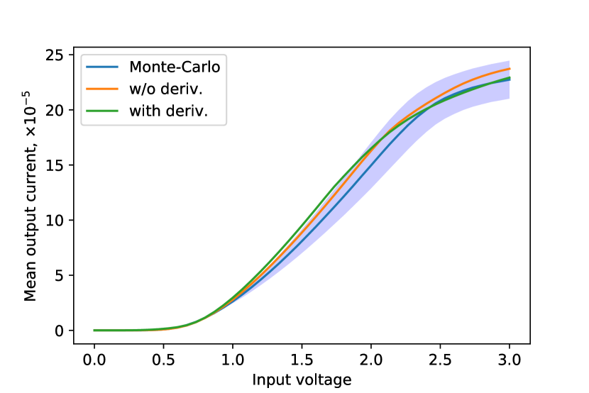
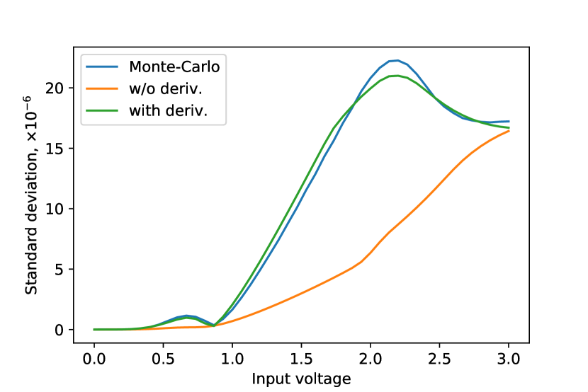
The value of output voltage is the function of interest. We approximate it by polynomials using Algorithm 1. The technique described is Sec. 5.2 is used to obtain derivatives. We use tensor product of univariate Hermite polynomials with weight function $w(x)=\exp\left(-x^{2}/2\right)$ as a set of basis functions because input random parameters have a normal distribution and their probability density function has the same form as $w(x)$. The mean value of the output signal coincides with the first component of $\alpha$, i.e. with the coefficient of the first polynomial $P_{0}(x)=0$. The standard deviation is equal to the square root of the sum of squares of the remaining components of the vector $\alpha$

$$\text{s.d.}=\left(\sum_{i=2}^{M}\alpha_{i}^{2}\right)^{1/2}$$

We compare the results of simulation in in two cases: with and without using derivatives. The number of points is equal to $9$ in both cases. In the case without using derivatives, we take $3$ basis polynomials, so the system matrix has size $9\times 3$. In the case of using derivatives, the number of basis polynomials is equal to $5$, the size of the matrix is $32\times 5$. Monte-Carlo simulation with $10^{5}$ samples is used as a reference. The results of the model simulation are shown in Fig 5. The mean values of the output voltage are close to each other, but one can see the advantages of the derivative approach when the values of derivatives are used along with the values of the function. Such small values of number of points and number of basis polynomials are used to show the difference between methods.

6 Partial differential equation

Our method can also be applied to the classical uncertainty quantification UQ problem for the partial differential equation. Let us consider the following differential equation, describing the stationary process of heat transfer

$$\operatorname{div}\left(k\,\operatorname{grad}u\right)=-F,$$

where the function $k$ is a given thermal conductivity, the function $F$ is a given heat source and $u$ is an unknown temperature distribution.

We consider the case when $k$ represents a lognormal random field

(11) $$k(x)=\exp(a+bg(x))$$

where $g$ is a standard Gaussian random field with the following correlation function

(12) $$\rho(x,\,y)=\exp\left(-\left\lVert x-y\right\rVert^{2}/\sigma^{2}\right).$$

For numerical experiments, the values of parameters $a$ and $b$ in (11) are $a=-0.0430888$, $b=0.29356$, so the mean value and the standard deviation of $k$ are $1$ and $0.3$, respectively. In (12), $\sigma=0.2$.

To model a random distribution of the thermal conductivity $k$, we use the Expansion Optimal Linear Estimation method [24]. According to this method, a random field is approximated by a truncated sum of the following form

(13) $$g(x)=\sum_{i=1}^{N}\frac{\xi_{i}}{\sqrt{l_{i}}}\left(\phi_{i},\,C_{x\eta}\right)$$

where i.i.d. $\xi_{i}\sim\mathcal{N}(0,1)$, $C_{x\eta}$ are vectors with elements $C^{i}_{x\eta}=\rho(x,\,\eta_{i})$, $l_{i}$ and $\phi_{i}$ are the eigenvalues and eigenvectors of the matrix $C_{\eta\eta}$ accordingly.

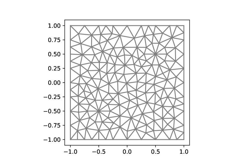
The number of terms in (13) is $N=40$ for the numerical experiments. The objective function $T$ is the average temperature in the circle $C$ with the center $(-0.5,\,-0.5)$ and the radius $0.2$

$$T=\int_{C}u\,ds,\quad C=\{x\in\mathbb{R}^{2}\colon\left(x+0.5\right)^{2}+\left(y+0.5\right)^{2}<0.2^{2}\}.$$

The heat source $F$ is equal $500$ in the circle with the center $(0.5,\,0.5)$ and the radius $0.2$, and $F=0$ elsewhere. The Python package dolfin-adjoint [3] is used for solving the partial differential equation and to obtain derivatives.

The mesh used in the experiment is shown in Fig 6. We use Monte-Carlo simulation with $N_{MC}=10^{4}$ samples as a reference. The results of numerical experiments are shown in Fig 7.

Figure 6: Mesh for finite-element method.

Figure 7: Cumulative distribution function of total temperature in the selected area.

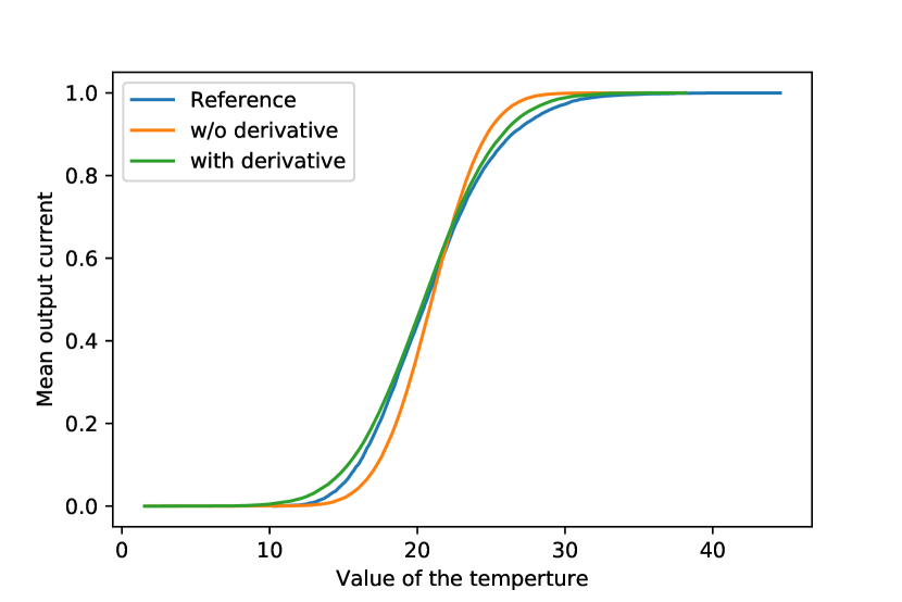
The sizes of the system matrices (4) in cases of not using derivatives and with derivatives are $20\times 176$ and $81\times 176\cdot 41$, respectively.

We take $p=0.5$, and the total number of the basis polynomials is $81$ when $q=2$. In the non-derivative case, we just truncate polynomials with high powers.

7 Possible difficulties of the derivative based approach

7.1 Singularity of system matrix

In some cases, the system matrix is not of a full column rank.

Let us consider a small matrix generated by two-dimensional tensor product of polynomials of cumulative degree no more than $2$ taken at two points. It has the form

$$A=\left(\begin{array}[]{cccccc}1&x_{1}&{y_{1}}&{x_{1}}{y_{1}}&x_{1}^{2}&y_{1}^{2}\\ 0&1&0&{y_{1}}&2{x_{1}}&0\\ 0&0&1&{x_{1}}&0&2{y_{1}}\\ 1&x_{2}&{y_{2}}&{x_{2}}{y_{2}}&x_{2}^{2}&y_{2}^{2}\\ 0&1&0&{y_{2}}&2{x_{2}}&0\\ 0&0&1&{x_{2}}&0&2{y_{2}}\\ \end{array}\right).$$

The rank of the matrix $A$ is $5$ as the rows $a_{i}$ for $i=1,\,\dots,6$ of the matrix are linearly dependent

$$-2a_{1}+(x_{1}-x_{2})a_{2}+(y_{1}-y_{2})a_{3}+2a_{4}+(x_{1}-x_{2})a_{5}+(y_{1}-y_{2})a_{6}=0.$$

A more complex example is the matrix of size $10\times 12$ generated by polynomials of cumulative degree no more than $2$ taken at three points

$$A=\left(\begin{array}[]{cccccccccc}1&x_{1}&y_{1}&z_{1}&x_{1}y_{1}&x_{1}z_{1}&y_{1}z_{1}&x_{1}^{2}&y_{1}^{2}&z_{1}^{2}\\ 0&1&0&0&y_{1}&z_{1}&0&2x_{1}&0&0\\ 0&0&1&0&x_{1}&0&z_{1}&0&2y_{1}&0\\ 0&0&0&1&0&x_{1}&y_{1}&0&0&2z_{1}\\ 1&x_{2}&y_{2}&z_{2}&x_{2}y_{2}&x_{2}z_{2}&y_{2}z_{2}&x_{2}^{2}&y_{2}^{2}&z_{2}^{2}\\ 0&1&0&0&y_{2}&z_{2}&0&2x_{2}&0&0\\ 0&0&1&0&x_{2}&0&z_{2}&0&2y_{2}&0\\ 0&0&0&1&0&x_{2}&y_{2}&0&0&2z_{2}\\ 1&x_{3}&y_{3}&z_{3}&x_{3}y_{3}&x_{3}z_{3}&y_{3}z_{3}&x_{3}^{2}&y_{3}^{2}&z_{3}^{2}\\ 0&1&0&0&y_{3}&z_{3}&0&2x_{3}&0&0\\ 0&0&1&0&x_{3}&0&z_{3}&0&2y_{3}&0\\ 0&0&0&1&0&x_{3}&y_{3}&0&0&2z_{3}\\ \end{array}\right)$$

The rank of this matrix $A$ is $9$.

This effect is also manifested in the matrices based on the polynomials of the maximal degree not more than some fixed value. Let $A$ be the $15\times 15$ matrix of the polynomials with the maximal power no more than $4$ taken at $5$ points. The rank of this matrix is $14$.

Thus, it limits from below the number of points we take in the derivative-based approach. At the moment we do not have explicit values of the rank and plan to study it in the future.

7.2 When matrix without derivatives works better

Let us consider a toy example of 1D function approximation at two points. Let $f(x)=\sin(x)$, evaluation points are $x_{0}=-\pi$ and $x_{1}=\pi$. We use a linear function $\widehat{f}(x)=kx+b$ to approximate $f$. The standard approach leads to the following linear system

$$\begin{pmatrix}1&-\pi\\ 1&\pi\end{pmatrix}\begin{pmatrix}b\\ k\end{pmatrix}=\begin{pmatrix}0\\ 0\end{pmatrix}$$

with solution $b=0$, $k=0$. The norms of the error of this approximation are

$$\left\lVert f-\widehat{f}\right\rVert_{2}=\int_{0}^{2\pi}\sin^{2}x\,dx\approx 1.77,\quad\left\lVert f-\widehat{f}\right\rVert_{\infty}=1.$$

The linear system of the LSM in derivative approach is the following

$$\begin{pmatrix}1&-\pi\\ 0&1\\ 1&\pi\\ 0&1\end{pmatrix}\begin{pmatrix}b\\ k\end{pmatrix}=\begin{pmatrix}0\\ -1\\ 0\\ -1\end{pmatrix}$$

with the solution

$$b=0,\quad k=-\frac{1}{1+\pi^{2}}.$$

In this approach the norms of the errors are

$$\left\lVert f-\widehat{f}\right\rVert_{2}\approx 2.11,\\ \quad\left\lVert f-\widehat{f}\right\rVert_{\infty}\approx 1.15.$$

One can see that both norms are worse in the derivative approach.

However, we can approximate our function with more than two basis polynomial in derivatives approach using the same number of points. Let $\widehat{f}(x)=a_{0}+a_{1}x+a_{2}x^{2}+a_{3}x^{3}$. Then, after solving the linear system, we get

$$a_{0}=0,\quad a_{1}=\frac{1}{2},\quad a_{2}=0,\quad a_{3}=-\frac{1}{2\pi^{2}},$$

and the corresponding errors are

$$\left\lVert f-\widehat{f}\right\rVert_{2}\approx 0.71,\\ \quad\left\lVert f-\widehat{f}\right\rVert_{\infty}\approx 0.43.$$

So, the advantages of the derivative approach are manifested in the case when we take an approximation polynomial of a higher degree than in the case without derivatives. Moreover, in the derivative approach we can generate a system matrix with a large ratio of the number of rows to the number of columns to obtain greater stability.

8 Related works

Our method is applicable only in the cases where the function can be approximated by a linear combination of fixed basis functions. The problem of function approximation using a preselected set of basis functions is the old and classical problem. For many classes of problems, including the approximation of smooth multivariate functions [30, 34], solutions of parametric PDEs [13], and uncertainty quantification [9, 16], approximation bounds are known. The interpolation and approximation of functions in this setting using adaptive function sampling have been studied in [31], including bounds on the Lebesgue constant for different basis sets in the multidimensional cases [21, 12].

There are several approaches to improve the accuracy of the approximation and to obtain theoretical estimates on it. In the paper [17] an approximation by smooth spline is considered in the multidimensional case. An adaptive algorithm is proposed which allows selecting domains of approximation. Errors estimations are given for this adaptive scheme.

The paper [16] considers the regularity of the polynomial approximation to the solution of parametric PDEs.

An approximation of the solutions of the parametric PDEs is also considered in the paper [15]. The solutions as functions of the parameters are holomorphic and highly anisotropic. The convergence rate of the approximation is established using these properties of the solution, which allows to avoid the curse of dimensionality.

A family of functions which are used for the approximation may not form an orthonormal basis. In connection with this, a problem of finding appropriate basis occur. In the paper [7] the approximation of functions in Hilbert space is considered. A greedy algorithm that allows selecting of the basis functions is proposed. Applications to the regression problem are considered. For a class of greedy algorithms convergence results are proven.

The classical paper [29] considers the interpolation of certain classes of multivariate functions. An efficient numerical algorithm is developed based on this study.

One of the ways to increase the accuracy of the approximation and reduce the number of points of function evaluation is finding appropriate sample points. The paper [27] presents an adaptive sparse grid stochastic collocation approach. Sparse grids interpolants are used to approximate solution as a function of input parameters. Univariate Leja sequence is suggested to use for a high-dimensional interpolation.

The classical problem of reconstruction of an unknown function by sampling in random points, and with the use of the least square method is considered in the paper [14]. A criterion on the number of approximating basis functions is presented. This criterion allows to ensure the stability of the LSM, and that the accuracy of the approximation is comparable to the best approximation. This criterion can be applied for different approximation schemes including trigonometric and algebraic polynomials approximation.

The paper [11] presents an algorithm for choosing points for the function interpolation. This method is applied in the adaptive fashion to different functions which are high-dimensional and have high evaluation cost.

The paper [19] investigates a weighted method of least squares in the application to the function approximation problem by truncating the polynomial chaos expansion. The weights are calculated on the basis of the selected points where the function is evaluated. These values correspond to the quadratures of integrals arising in the coefficient estimation. Such an approach leads to the stability and high accuracy of the approximation.

The integration problem of a multivariate function is solved in the paper [28] by using quasi-Monte Carlo (QMC) method. The authors identify classes of functions for which the effect of dimension is negligible. It is proved that the error in the worst case does not depend on the number of dimensions under certain conditions.

In the paper [23] several methods of avoiding the curse of dimensionality are considered in an application to the problem of integration over the $d$-dimensional cube.

The problems of multivariate function approximation and integration are considered in the paper [22]. It is proved that the studied integration schemes are strongly tractable for a certain set of weighted function spaces.

In the survey [10] the theory and applications of sparse grids are presented. The authors focus on the solution of partial differential equations. Several estimations on the number of degrees of freedom are considered. An extension to non-smooth solutions is made by adaptive update methods.

In our research, we rely on the fast methods for derivative computation which have attracted tremendous attention in the recent years in the field of machine learning. Many modern packages like TensorFlow [6] and Pytorch [4] implement such tools.

9 Conclusions and future work

In the present paper advantages of multivariate function interpolation with the use of the information about its derivatives are demonstrated. Several numerical experiments are conducted including ODE and PDE equations with coefficients depending on multidimensional parameters.

As a subject of future work, we consider the task of determining the optimal relation between the number of sample points and the number of the basis functions to increase stability and accuracy of the proposed scheme. The problem of finding optimal points set of function evaluation is in our plans as well. Additionally, we want to investigate convergence and stability bounds when the number of points increases. Also, it is crucial to determine theoretical estimates for the Lebesgue constants for the derivative approach.

References

- [1] Ahkab python package. https://ahkab.github.io/ahkab/. [online] [Accessed: 2017-03-20].
- [2] Autograd python library. https://github.com/HIPS/autograd/. [online] [Accessed: 2017-11-01].
- [3] Dolfin-adjoin project. http://www.dolfin-adjoint.org/en/latest/. [online] [Accessed: 2017-11-01].
- [4] Pytorch python framework. https://www.tensorflow.org/. [online] [Accessed: 2017-11-01].
- [5] ”rect maxvol“ algorithm. https://bitbucket.org/muxas/rect_maxvol. [online] [Accessed: 2017-11-01].
- [6] Tensorflow library. https://www.tensorflow.org/. [online] [Accessed: 2017-11-01].
- [7] A. R. Barron, A. Cohen, W. Dahmen, and R. A. DeVore, Approximation and learning by greedy algorithms, Ann. Stat., 36 (2008), pp. 64–94.
- [8] W. Baur and V. Strassen, The complexity of partial derivatives, Theor. Comput. Sci., 22 (1983), pp. 317–330.
- [9] G. Blatman and B. Sudret, Adaptive sparse polynomial chaos expansion based on least angle regression, Journal of Computational Physics, 230 (2011), pp. 2345–2367.
- [10] H.-J. Bungartz and G. Michael, Sparse grids, Acta Numer., 13 (2004), pp. 1–123.
- [11] E. Burnaev, I. Panin, and B. Sudret, Efficient design of experiments for sensitivity analysis based on polynomial chaos expansions, Ann. Math. Artif. Intel., 81 (2017), pp. 187–207.
- [12] J.-P. Calvi and V. M. Phung, On the lebesgue constant of Leja sequences for the unit disk and its applications to multivariate interpolation, J. Approx Theory, 163 (2011), pp. 608–622.
- [13] A. Chkifa, A. Cohen, and C. Schwab, High-dimensional adaptive sparse polynomial interpolation and applications to parametric PDEs, Found. Comput. Math., 14 (2014), pp. 601–633.
- [14] A. Cohen, M. A. Davenport, and D. Leviatan, On the stability and accuracy of least squares approximations, Found. Comput. Math., 13 (2013), pp. 819–834.
- [15] A. Cohen and R. DeVore, Approximation of high-dimensional parametric PDEs, Acta Numer., 24 (2015), pp. 1–159.
- [16] A. Cohen, R. DeVore, and C. Schwab, Analytic regularity and polynomial approximation of parametric and stochastic elliptic PDE’s, Anal. Appl., 9 (2011), pp. 11–47.
- [17] W. A. Dahmen, Adaptive approximation by multivariate smooth splines, J. Approx Theory, 36 (1982), pp. 119–140.
- [18] D. Dung, N. V. Temlyakov, and T. Ullrich, Hyperbolic cross approximation, (2016), https://arxiv.org/abs/1601.03978.
- [19] S. Ghili and G. Iaccarino, Least squares approximation of polynomial chaos expansions with optimized grid points, SIAM J. Sci. Comput., 39 (2017), pp. A1991–A2019.
- [20] A. Griewank, Achieving logarithmic growth of temporal and spatial complexity in reverse automatic differentiation, Optimization Methods and Software, 1 (1992), pp. 35–54.
- [21] M. Gunzburger and A. L. Teckentrup, Optimal point sets for total degree polynomial interpolation in moderate dimensions, (2014), https://arxiv.org/abs/1407.3291.
- [22] F. J. Hickernell and H. Wozniakowski, Integration and approximation in arbitrary dimensions, Adv. Comput. Math., 12 (2000), pp. 25–58.
- [23] F. Y. Kuo and I. Sloan, Lifting the curse of dimensionality, Not. Am. Math. Soc., 52 (2005), pp. 1320–1328.
- [24] C.-C. Li and A. D. Kiureghian, Optimal discretization of random fields, J. Eng. Mech., 119 (1993), pp. 1136–1154.
- [25] M. D. Mckay, R. Beckman, and W. Conover, A comparison of three methods for selecting vales of input variables in the analysis of output from a computer code, Technometrics, 21 (1979), pp. 239–245.
- [26] A. Mikhalev and I. V. Oseledets, Rectangular maximum-volume submatrices and their applications, Linear Algebra Appl., 538 (2018), pp. 187–211.
- [27] A. Narayan and J. D. Jakeman, Adaptive Leja sparse grid constructions for stochastic collocation and high-dimensional approximation, SIAM J. Sci. Comput., 36 (2014), pp. A2952–A2983.
- [28] I. H. Sloan and H. Wozniakowski, When are quasi-monte carlo algorithms efficient for high dimensional integrals?, J. Complexity, 14 (1998), pp. 1–3.
- [29] S. A. Smolyak, Quadrature and interpolation formulas for tensor products of certain classes of functions, Dokl. Akad. Nauk SSSR, 148 (1963), pp. 1042–1045.
- [30] V. N. Temljakov, Approximation of periodic functions of several variables with bounded mixed difference, Math. USSR Sb., 41 (1982), pp. 53–66.
- [31] M. Van Barel and M. Humet, Good point sets and corresponding weights for bivariate discrete least squares approximation, Dolomites Research Notes on Approximation, 8 (2015), pp. 37–50.
- [32] Z. Zhang, T. A. El-Moselhy, I. M. Elfadel, and L. Daniel, Stochastic testing method for transistor-level uncertainty quantification based on generalized polynomial chaos, IEEE T. Comput. Aid. D., 32 (2013), pp. 1533–1545.
- [33] Z. Zhang, X. Yang, I. V. Oseledets, G. E. Karniadakis, and L. Daniel, Enabling high-dimensional hierarchical uncertainty quantification by ANOVA and tensor-train decomposition, IEEE T. Comput. Aid. D., 34 (2014), pp. 63–76.
- [34] D. Zung, Approximation of classes of smooth functions of several variables, Journal of Soviet Mathematics, 35 (1986), pp. 2859–2875.