Optimal consensus control of the Cucker-Smale model

Abstract

We study the numerical realisation of optimal consensus control laws for agent-based models. For a nonlinear multi-agent system of Cucker-Smale type, consensus control is cast as a dynamic optimisation problem for which we derive first-order necessary optimality conditions. In the case of a smooth penalisation of the control energy, the optimality system is numerically approximated via a gradient-descent method. For sparsity promoting, non-smooth $\ell_{1}$-norm control penalisations, the optimal controllers are realised by means of heuristic methods. For an increasing number of agents, we discuss the approximation of the consensus control problem by following a mean-field modelling approach.

1 Introduction

This paper addresses centralised control problems for second-order, nonlinear, multi-agent systems (MAS). In such dynamics, the state of each agent is characterised by a pair $(x_{i},v_{i})$, representing variables which we refer to as position and velocity, respectively. The uncontrolled system consists of simple binary interaction rules between the agents, such as attraction, repulsion, and alignment forces. This commonly leads to self-organisation phenomena, flocking or formation arrays. However, this behaviour strongly depends on the cohesion of the initial configuration of the system, and therefore control design is relevant in order to generate an external intervention able to steer the dynamics towards a desired configuration. For second-order MAS, it is of particular interest the study of consensus emergence and control. In this context, we understand consensus as a travelling formation in which every agent has the same velocity. Self-organised consensus emergence for the Cucker-Smale model, see Cucker and Smale (2007), has been already characterised in Ha and Liu (2009); Carrillo et al. (2010a). The problem of consensus control for Cucker-Smale type models has been discussed in Caponigro et al. (2013); Bongini et al. (2015). A related problem is the design of controllers achieving a given formation, which has been previously addressed in Perea et al. (2009); Borzì and Wongkaew (2015).

Contributions. In this work we focus on the design of centralised control laws enforcing consensus emergence. For this, we cast the consensus control problem in the framework of optimal control theory, for which an ad-hoc computational methodology is presented. We consider a finite horizon control problem, in which the deviation of the population with respect to consensus is penalised along a quadratic control term. We derive first-order optimality conditions, which are then numerically realised via the Barzilai-Borwein (BB) gradient descent method. While the use of gradient methods is a standard tool for the numerical approximation of optimal control laws, see Borzì and Schulz (2011), the use of the BB method for large-scale agent-based models is relatively recent, Deroo et al. (2012), and we report on its use as a reliable method for optimal consensus control problems (OCCP) in nonlinear MAS. While the control performance is satisfactory, our setting allows the controller to act differently on every agent at every instant. The question of a more parsimonious control design remains open. As an extension of the proposed methodology, we address the finite horizon OCCP with a non-smooth, sparsity-promoting control penalisation. This control synthesis is sparse, acting on a few agents over a finite time frame, however its numerical realisation is far more demanding due to the lack of smoothness in the cost functional. To circumvent this difficulty, we propose a numerical realisation of the control synthesis via metaheuristics related to particle swarm optimisation (PSO), and to nonlinear model predictive control (NMPC). Finally, based on the works Carrillo et al. (2010a, b); Fornasier and Solombrino (2014); Bongini et al. (2017); Albi et al. (2017a, 2016); Albi and Kalise (2018), we discuss the resulting mean-field optimal control problem: that obtained as the number of agents $N$ tends to $\infty$ and the micro-state $(x_{i}(t),v_{i}(t))$ of the population is replaced by an agent density function $f(t,x,v)$.

Structure of the paper. In Section 2 we revisit the Cucker-Smale model and results on consensus emergence and control. In Section 3 we address the OCCP via first-order necessary optimality conditions and its numerical realisation. Section 4 introduces the sparse OCCP and its approximation. Concluding, in Section 5 we present a mean-field modelling approach for OCCP when the number of agents is sufficiently large.

2 The Cucker-Smale model and consensus emergence

We consider a set of $N$ agents with state $(x_{i}(t),v_{i}(t))\in\mathbb{R}^{d}\times\mathbb{R}^{d}$, where $d$ is the dimension of the physical space, interacting under second-order Cucker-Smale dynamics

$$\frac{dx_{i}}{dt} =v_{i}\,,\quad\frac{dv_{i}}{dt}=\frac{1}{N}\sum_{j=1}^{N}a(\|x_{i}-x_{j}\|)(v_{j}-v_{i})$$ (2.1)

$$\mathbf{x}(0) =\mathbf{x}_{0}\,,\quad\mathbf{v}(0)=\mathbf{v}_{0}\,,$$ (2.2)

where $a(r)$ is a communication kernel of the type

$$a(r)=\frac{K}{(1+r^{2})^{\beta}}\,,\qquad\beta\geq 0\,,K>0\,,$$ (2.3)

and we use the notation $\mathbf{x}(t)=(x_{1}(t),\ldots,x_{N}(t))^{t}$, $\mathbf{v}(t)=(v_{1}(t),\ldots,v_{N}(t))^{t}\in\mathbb{R}^{dN}$. Both $\|\cdot\|$ and $\|\cdot\|_{2}$ are indistinctly used for the $\ell_{2}$-norm, while $\|\cdot\|_{1}$ stands for the $\ell_{1}$-norm. We will focus on the study of consensus emergence, i.e. the convergence towards a configuration in which

$$v_{i}=\bar{v}=\frac{1}{N}\sum_{j=1}^{N}v_{j}\,\quad\forall i.$$ (2.4)

Note that although the interaction kernel $a(r)$ decays as the distance between agents increasing, the interconnection topology remains unchanged, i.e., all the agents interaction with all the agents in the swarm at all times. For a system of the type (2.1)-(2.2), a consensus configuration will remain as such without any external intervention, and positions will evolve in planar formation. The emergence of consensus as a self-organisation phenomenon, either by a sufficiently cohesive initial configuration $(\mathbf{x}_{0},\mathbf{v}_{0})$ or a strong interaction $a(r)$, is a problem of interest in its own right. To study consensus emergence, it is useful to define the form $B:\mathbb{R}^{dN}\times\mathbb{R}^{dN}\to\mathbb{R}$

$$B(\mathbf{w},\mathbf{v})=\frac{1}{2N^{2}}\sum_{i,j=1}^{N}\|w_{i}-v_{j}\|^{2}\,.$$

Note that for a population in consensus, $B(\mathbf{v},\mathbf{v})\equiv 0$. A solution $(\mathbf{x}(t),\mathbf{v}(t))$ to (2.1)-(2.2) tends to a consensus configuration if and only if

$$V(t):=B(\mathbf{v}(t),\mathbf{v}(t))\rightarrow 0\quad\text{ as }\quad t\rightarrow+\infty.$$

Analogously, we define $X(t):=B(\mathbf{x}(t),\mathbf{x}(t))$. We briefly recall some well-known results on self-organised consensus emergence.

Theorem 1

Unconditional consensus emergence (Cucker and Smale (2007); Carrillo et al. (2010b)). Given an interaction kernel $a(r)=\frac{K}{(1+r^{2})^{\beta}}$ with $K>0$ and $0\leq\beta\leq\frac{1}{2}$, the Cucker-Smale dynamics (2.1)-(2.2) convergence asymptotically to consensus, i.e. $V(0)\leq e^{-\lambda t}V(t)$, for $\lambda>0$.

Theorem 2

Conditional consensus emergence (Ha and Liu (2009); Ha et al. (2010)). For $a(r)=\frac{K}{(1+r^{2})^{\beta}}$ with $K>0$ and $\frac{1}{2}\leq\beta$, if

$$\sqrt{V(0)}<\int\limits_{\sqrt{X(0)}}^{+\infty}a(2\sqrt{N}s)\,ds\,,$$

then the Cucker-Smale dynamics (2.1)-(2.2) convergence asymptotically to consensus.

In this work we are concerned with inducing consensus through the synthesis of an external forcing term $\mathbf{u}(t)=(u_{1}(t),\ldots,u_{N}(t))^{t}$ in the form

$$\frac{dx_{i}}{dt} =v_{i}\,,$$ (2.5)

$$\frac{dv_{i}}{dt} =\frac{1}{N}\sum_{j=1}^{N}a(\|x_{i}-x_{j}\|)(v_{j}-v_{i})+u_{i}(t)\,,$$ (2.6)

$$x_{i}(0) =x_{0}\,,\quad v_{i}(0)=v_{0}\,,\qquad i=1,\ldots,N\,,$$ (2.7)

where the control signals $u_{i}\in{\mathcal{U}}=\{u:\mathbb{R}_{+}\longrightarrow U\}$ and $U$ a compact subset of $\mathbb{R}^{d}$.

3 The optimal control problem and first-order necessary conditions

In this section we entertain the problem of obtaining a centralised forcing term $\mathbf{u}(t)$ which will either induce consensus on an initial configuration $(\mathbf{x}_{0},\mathbf{v}_{0})$ that would otherwise diverge, or which accelerates the rate of convergence for initial data that would naturally self-organise. Formally, for $T>0$ and given a set of admissible control signals ${\mathcal{U}}^{N}:\mathbb{R}^{+}_{0}\to[L^{\infty}(0,T;\mathbb{R}^{d})]^{N}$ for the entire population, we seek a solution to the minimisation problem

$$\underset{\mathbf{u}(\cdot)\in{\mathcal{U}}^{N}}{\min}\mathcal{J}(\mathbf{u}(\cdot);\mathbf{x}_{0},\mathbf{v}_{0}):=\int_{0}^{T}\ell(\mathbf{v}(t),\mathbf{u}(t))\,dt\,,$$ (3.8)

with the running cost defined as

$$\ell(\mathbf{v},\mathbf{u}):=\frac{1}{N}\sum_{j=1}^{N}\left(\left\|\bar{v}-v_{j}\right\|^{2}+\gamma\left\|u_{j}\right\|^{2}\right),$$ (3.9)

with $\gamma>0$, subject to the dynamics (2.5)-(2.7).

3.1 First-order optimality conditions

While existence of a minimiser $\mathbf{u}^{*}$ of (3.8) follows from the smoothness and convexity properties of the system dynamics and the cost, the Pontryagin Minimum Principle Pontryagin et al. (1962) yields first-order necessary conditions for the optimal control. Let $(p_{i}(t),q_{i}(t))\in\mathbb{R}^{d}\times\mathbb{R}^{d}$ be adjoint variables associated to $(x_{i},v_{i})$, then the optimality system consists of a solution $(\mathbf{x}^{*},\mathbf{v}^{*},\mathbf{u}^{*},\mathbf{p}^{*},\mathbf{q}^{*})$ satisfying (2.5)-(2.7) along with the adjoint equations

$$-\frac{dp_{i}}{dt} =\frac{1}{N}\sum_{j=1}^{N}\frac{a^{\prime}\left(\left\|x_{j}-x_{i}\right\|\right)}{\left\|x_{j}-x_{i}\right\|}\left\langle q_{j}-q_{i},v_{j}-v_{i}\right\rangle\left(x_{j}-x_{i}\right)\,,$$ (3.10)

$$-\frac{dq_{i}}{dt} =p_{i}+\frac{1}{N}\sum_{j=1}^{N}a\left(\left\|x_{j}-x_{i}\right\|\right)\left(q_{j}-q_{i}\right)-\frac{2}{N}\left(\bar{v}-v_{i}\right),$$ (3.11)

$$p_{i}(T) =0\,,\quad q_{i}(T)=0\,,\qquad i=1,\ldots,N\,,$$ (3.12)

and the optimality condition

$$\mathbf{u}(t)=\underset{\mathbf{w}\in\mathbb{R}^{dN}}{argmin}\sum_{j=1}^{N}\left(\left\langle q_{j},\frac{dv_{j}}{dt}\right\rangle+\frac{\gamma}{N}\left\|w_{j}\right\|^{2}\right)=-\frac{N}{2\gamma}\mathbf{q}^{t}\,.$$ (3.13)

3.2 A gradient-based realisation of the optimality system

The adjoint system (3.10)-(3.13) is used to implement a gradient descent method for the numerical realisation of the optimal control law. It can be readily verified that the gradient of the cost $\mathcal{J}$ in (3.8) is given by

$$\nabla\mathcal{J}\left(\mathbf{u}\right)=\mathbf{q}^{t}+\frac{2\gamma}{N}\mathbf{u}\,,$$ (3.14)

obtained by differentiating (3.13) with respect to $\mathbf{u}$. With this expression for $\nabla\mathcal{J}$, the gradient iteration is presented in Algorithm 1.

Algorithm 1 Gradient descent method with BB update.

$tol>0$, $k_{\mathrm{max}}$, $\mathbf{u}^{0}$, $\mathbf{u}^{-1}$.

$k=0$;

while $\left\|\nabla\mathcal{J}\left(\mathbf{u}^{k}\right)\right\|>tol$ and $k<k_{\mathrm{max}}$ do

     1) Obtain $(\mathbf{x}^{k},\mathbf{v}^{k})$ from (2.5)-(2.7) with $\mathbf{u}^{k}$;

     2) Obtain $(\mathbf{p}^{k},\mathbf{q}^{k})$ from (3.10)-(3.12) with $(\mathbf{x}^{k},\mathbf{v}^{k})$;

     3) Evaluate the gradient $\nabla\mathcal{J}\left(\mathbf{u}^{k}\right)$ as in (3.14);

     4) Compute the step

$$\alpha_{k}:=\frac{\left\langle\mathbf{u}^{k}-\mathbf{u}^{k-1},\nabla\mathcal{J}\left(\mathbf{u}^{k}\right)-\nabla\mathcal{J}\left(\mathbf{u}^{k-1}\right)\right\rangle}{\left\|\nabla\mathcal{J}\left(\mathbf{u}^{k}\right)-\nabla\mathcal{J}\left(\mathbf{u}^{k-1}\right)\right\|^{2}}\,;$$ (3.15)

     5) Update $\mathbf{u}^{k+1}=\mathbf{u}^{k}-\alpha_{k}\nabla\mathcal{J}\left(\mathbf{u}^{k}\right)$;

     6) $k:=k+1$;

end while

In Algorithm 1, the gradient is first obtained by integrating the forward-backward optimality system, and then the step $\alpha_{k}$ in 4) is chosen as in the Barzilai-Borwein method, see Barzilai and Borwein (1988).

3.3 Numerical experiments

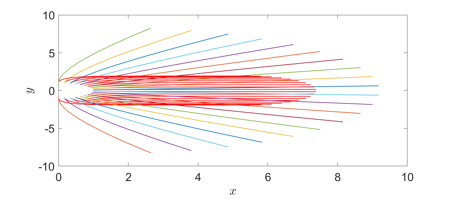
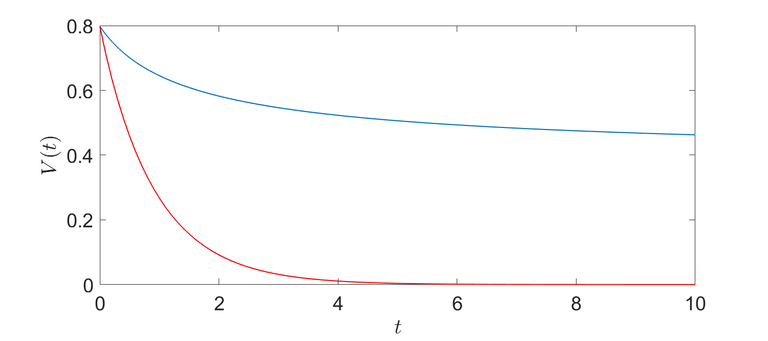
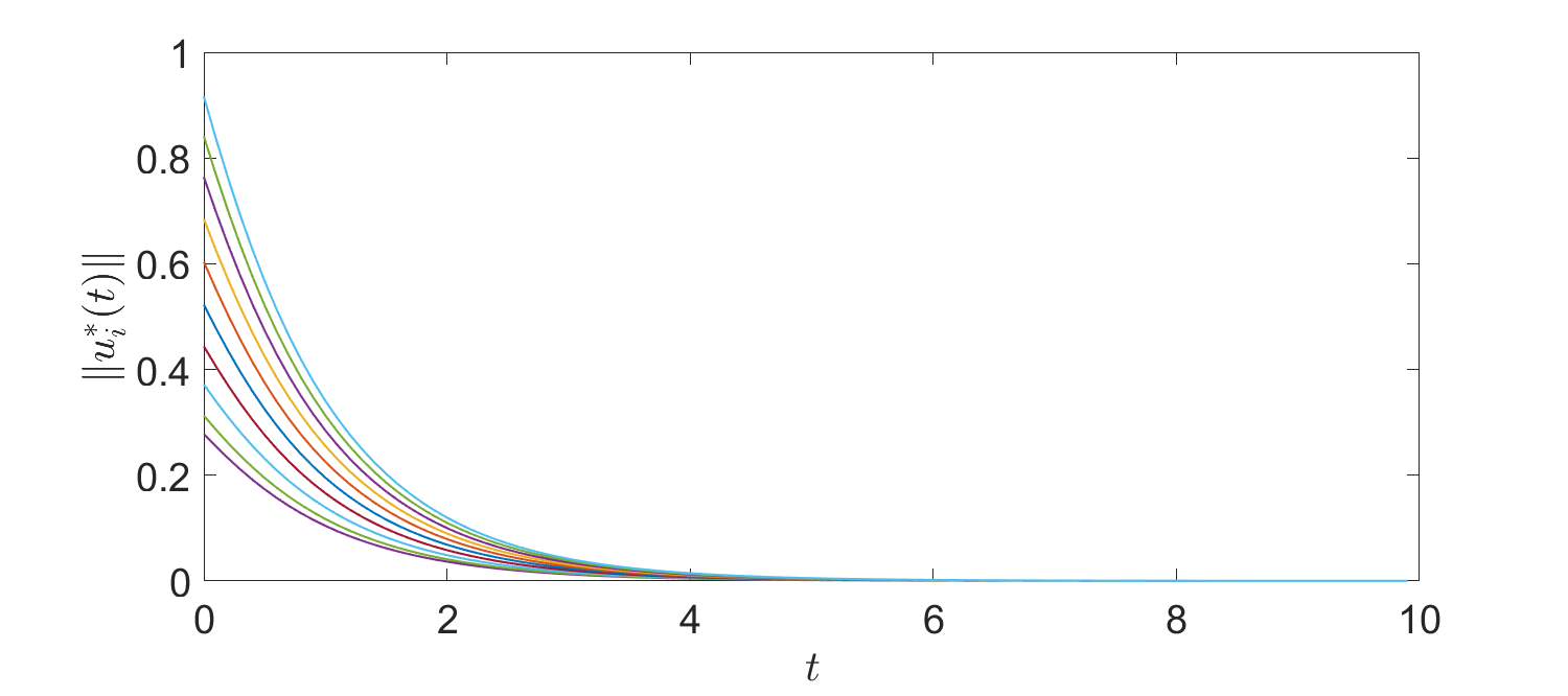
Figure 3.1: Free vs. controlled (shown in red) dynamics. Top: trajectories. Middle: functional $V(t)$. Bottom: norm of the optimal control $u_{i}^{*}(t)$ for each agent.

Figure 3.1 shows a comparison of the free two-dimensional dynamics of a sample initial condition $(\mathbf{x}_{0},\mathbf{v}_{0})$ and the system under an approximation to the optimal control $\mathbf{u}^{*}$ found with this algorithm. A Runge-Kutta 4th order scheme was used to integrate the differential equations for the state and the adjoint with end time $T=10$, time step $dt=0.1$ (resulting on $N_{T}=51$ points for the time discretisation), and a stopping tolerance for the gradient norm of $10^{-3}$. The condition $(\mathbf{x}_{0},\mathbf{v}_{0})$ is chosen such that consensus would not be reached naturally; long-time numerics of the free system show that $V(t)$ converges to an asymptotic value around $\bar{V}=0.4$. In the controlled setting, consensus is reached rapidly as can be seen from the trajectories themselves, as well as from the fast convergence of the functional $V(t)$ to zero. Furthermore, the norm of the control also decreases in time as the system is steered towards and into the self-organisation region.

4 The sparse consensus control and its approximation via heuristics

In this section, we address the problem of enforcing sparsity on the optimal consensus strategy. As shown in Albi et al. (2017b); Bongini and Fornasier (2014); Caponigro et al. (2013); Kalise et al. (2017), one way to do it is by using as control cost the $\ell_{1}$-norm $\|\cdot\|_{1}$ in the minimisation problem (3.8), instead of the standard squared $\ell_{2}$-norm $\|\cdot\|_{2}^{2}$. However, the choice of the non-differentiable control cost $\|\cdot\|_{1}$ gives rise to a non-smooth cost functional $\mathcal{J}$, for which gradient-based numerical solvers like the one presented in Section 3.2 are not directly suitable. To circumvent the non-smoothness of $\mathcal{J}$, we shall resort to a metaheuristic procedure known as particle swarm optimisation (PSO).

4.1 Particle Swarm optimisation

First introduced in Kennedy and Eberhart (1995); Shi and Eberhart (1998), PSO is a numerical procedure that solves a minimisation problem by iteratively trying to improve a candidate solution. PSO solves the problem by generating a population of points in the discrete control state space of solutions $\mathcal{U}^{N}=\mathbb{R}^{d\times N\times N_{T}}$ called particles. Each particle is treated as a point in this $D=d\times N\times N_{T}$-dimensional space with coordinates $(z_{i1},\ldots,z_{iD})$, and the cost functional is evaluated at each of these points. The best previous position (i.e., the one for which the cost functional is minimal) of any particle $(m_{i1},\ldots,m_{iD})$ is recorded, together with the index $h$ of the best particle among all the particles. We let then the particles evolve according to the system

$$z_{ij} :=z_{ij}+w_{ij},$$

$$w_{ij} :=w_{ij}+c_{1}\xi(m_{ij}-z_{ij})+c_{2}\eta(m_{hj}-z_{ij}),$$

where $c_{1},c_{2}>0$ are two constant parameters and $\xi,\eta$ are two random variables with support in $[0,1]$. PSO is a metaheuristic since it makes few or no assumptions about the problem being optimised and can search very large spaces of candidate solutions: in particular, PSO does not use the gradient of the problem being optimised, which means PSO does not require that the optimisation problem be differentiable. However, it yields to a decrease of the cost function. Notice that whenever the dimension of the control space $D$ is very large (that is, either $d$, $N$ or $N_{T}$ are large), the problem suffers from the curse of dimensionality, as the evaluation of $\mathcal{J}$ at all the particles and the subsequent search for the best position becomes prohibitively expensive. To mitigate this difficulty, we shall optimise within a nonlinear model predictive control (NMPC) loop with short prediction horizon.

4.2 Nonlinear Model Predictive Control

For a prediction horizon of $H$ steps, for $k=1,\ldots,N_{T}-H$ and a discrete time version of the dynamics (2.1)-(2.2), we minimise the following performance index

$$\sum^{H}_{h=0}\frac{1}{N}\sum^{N}_{j=1}\bigg{(}\|\overline{v}^{k+h}-v^{k+h}_{j}\|_{2}^{2}+\gamma\|u^{k+h}_{j}\|^{r}_{r}\bigg{)},$$ (4.16)

for some $\ell_{r}$-norm with $r\geq 1$, generating a sequence of controls $(\mathbf{u}^{k},\mathbf{u}^{k+1},\ldots,\mathbf{u}^{k+H})$ from which only the first term $\mathbf{u}^{k}$ is taken to evolve the dynamics from $k$ to $k+1$. The system’ state is sampled again and the calculations are repeated starting from the new current state, yielding a new control and a new predicted state path. Although this approach is suboptimal with respect to the full time frame optimisation presented in Section 3, in practice it produces very satisfactory results.

For $H=1$, the NMPC approach recovers an instantaneous controller, whereas for $H=N_{T}-1$ it solves the full time frame problem (3.8). Such flexibility is complemented with a robust behaviour, as the optimisation is re-initialised every time step, allowing to address perturbations along the optimal trajectory. For further references, see Mayne et al. (2000).

4.3 Numerical experiments

We now report the results of the numerical simulations of (3.8) with $\|\cdot\|_{1}$ and $\|\cdot\|_{2}^{2}$ together with the setup PSO-NMPC described above. The aim is to check whether the optimal control obtained with the $\ell_{1}$-control cost is sparser than the one obtained with the $\ell_{2}$-norm. To do so, we shall compare their norms at each time, since a sparse control will be equal to 0 most of the time. Starting from an initial configuration $(\mathbf{x}_{0},\mathbf{v}_{0})$ that does not converge to consensus, we compare the effect of a different NMPC horizon $H\in\{3,10\}$ and of a different $\ell_{r}$-control cost for $r\in\{1,2\}$ in (4.16) on the optimal control strategy.

We test the PSO-NMPC procedure with $H=3$ periods ahead instead of the full time frame. Figure 4.2 shows the controlled dynamics of the agents with the optimal control obtained for $r=1$ (top) and $r=2$ (bottom). Both controls decisively improve the alignment behaviour with respect to the uncontrolled dynamics. Figure 4.3 shows the behaviour of the $V$ functional: for both controlled dynamics, the velocity spread $V(t)$ goes steadily to 0. To see how sparse the controls are, for each control strategy in Figure 4.4 we show the corresponding heat map, i.e., the matrix $\mathcal{H}$ such that $\mathcal{H}_{ik}$ contains the norm of the control acting on the $i$-th agent at step $k$. The stronger the control, the brighter the entry shall be: we can notice that the heat map for $r=1$ is sparser than the one for $r=2$, being concentrated on few bright spots. This corroborates the findings of Bongini and Fornasier (2014); Caponigro et al. (2013), where the sparsifying powers of an $\ell_{1}$-control cost were shown.

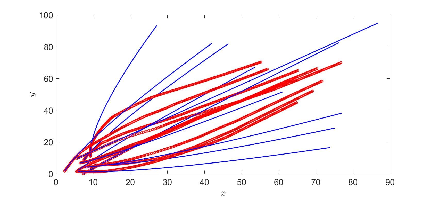
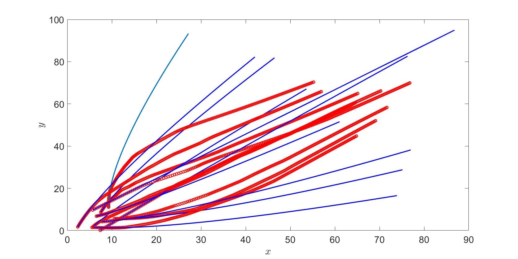
Figure 4.2: Controlled dynamics for $H=3$. Top: agents’ dynamics for $r=1$. Bottom: agents’ dynamics for $r=2$.

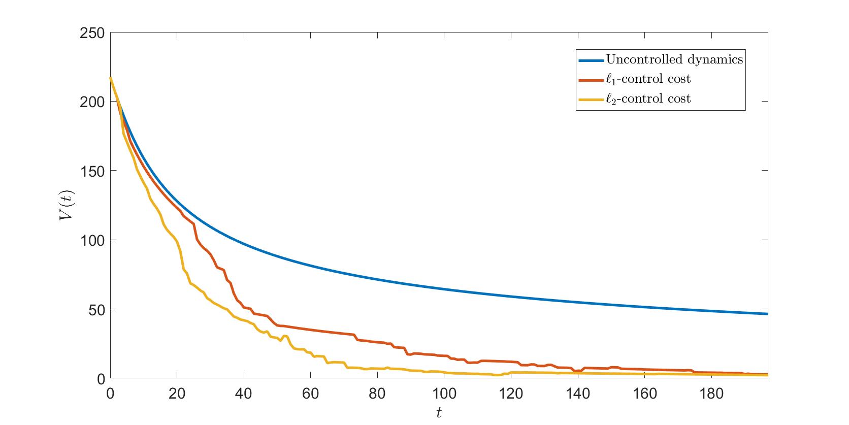
Figure 4.3: Functional $V(t)$ for $H=3$. Blue: uncontrolled dynamics. Red: $\ell_{1}$-cost. Yellow: $\ell_{2}$-cost.

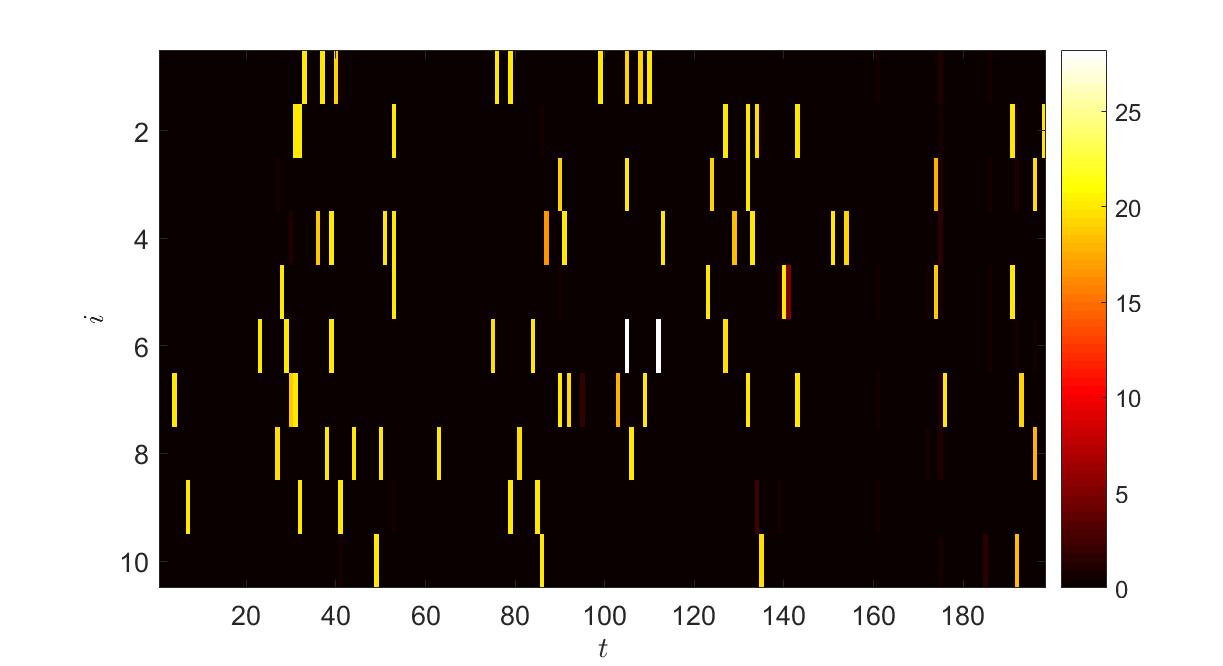
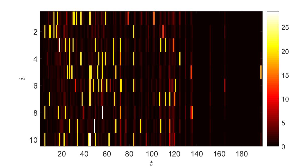
Figure 4.4: Heat map of control strategies for $H=3$, control action in time for each agent. Top: the case of $r=1$. Bottom: the case of $r=2$.

5 The Continuous Control Problem

We consider the continuous control problem that results in the limit of the discrete problem from Section 3 as $N\rightarrow\infty$. Formally, the forced Cucker-Smale dynamics (2.5)-(2.7) can be written as a Vlasov-type transport equation

$$\frac{\partial f}{\partial t}+\left(v\cdot\nabla_{x}\right)f+\nabla_{v}\cdot\left[\left(A(x,v)*f+u(t,x,v)\right)f\right]=0,$$ (5.17)

where $A(x,v)=a(|x|)v$ and $f,u:[0,T]\times\mathbb{R}^{2}\times\mathbb{R}^{2}\rightarrow\mathbb{R}$ are the probability density for the state and a forcing term, respectively. An equivalent minimisation problem can be posed:

$$\underset{u\in{\mathcal{U}}}{\min}\mathcal{J}(u;f_{0}):=\int_{0}^{T}\ell(f,u)\,dt\,,$$ (5.18)

for fixed $T>0$ and a running cost $\ell(f,u)$ given by the expression:

$$\int_{\mathbb{R}^{2d}}\left\|v-\int_{\mathbb{R}^{2d}}w\,df(y,w)\right\|^{2}+\gamma\left\|u(t,x,v)\right\|^{2}\,df(x,v).$$ (5.19)

The solutions of the discrete control problem (3.8) converge to that of the continuous problem (5.17), as discussed in Fornasier and Solombrino (2014). This can be verified numerically by fixing an initial distribution $f_{0}$ and studying the sequence solutions of the discrete problem with initial conditions sampled from said distribution; a subsequence is known to converge as $N\rightarrow\infty$. Besides the solution, the optimal value of the objective functional $\mathcal{J}^{*}_{N}$ is also expected to converge, which can be verified. Initial conditions without natural consensus were constructed by sampling $x$ from a superposition of two Gaussian distributions and letting $x=v$. The marginal distributions of $f_{0}$ on $x$ and in $v$ are shown in Figure 5.5. A sequence of such discrete problems were solved for several values of $N$. Figure 5.6 shows the comparison between the free and controlled trajectories for various values of $N$. The Runge-Kutta scheme was used to solve the differential equations for the state and the adjoint with end time $T=5$, time step $dt=0.1$ (resulting on $51$ points for the time discretisation), and a stopping tolerance of $10^{-2}$. Figure 5.7 shows the evolution of the optimal cost $\mathcal{J}^{*}_{N}$, which appears to be of order $\mathcal{J}^{*}_{N}\sim\mathcal{O}(1)$ as expected for the convergence as $N\rightarrow\infty$. Figure 5.8 shows the marginal distribution of $f(T)$ on $v$ for the free and forced settings with the same scale; the controlled case yields a singular distribution indicating consensus. Figure 5.9 shows a heat map of the optimal control $u_{i}^{*}(t)$. We observed that the average norm of the control is of $\sim\mathcal{O}(1)$ as $N\rightarrow\infty$; furthermore the time at which the control is nearly zero is roughly constant for large $N$. Table 5.1 shows the evolution of the number of optimisation iterations (i.e. loops on Algorithm 1) as well as the computation CPU time in hours; notice that the number of iterations remains roughly constant, while the computation time scales quadratically in $N$.

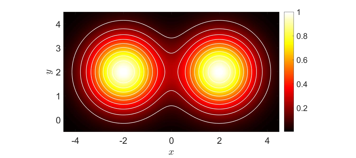
Figure 5.5: Marginal distribution of $f_{0}$ on $x$ and $v$.

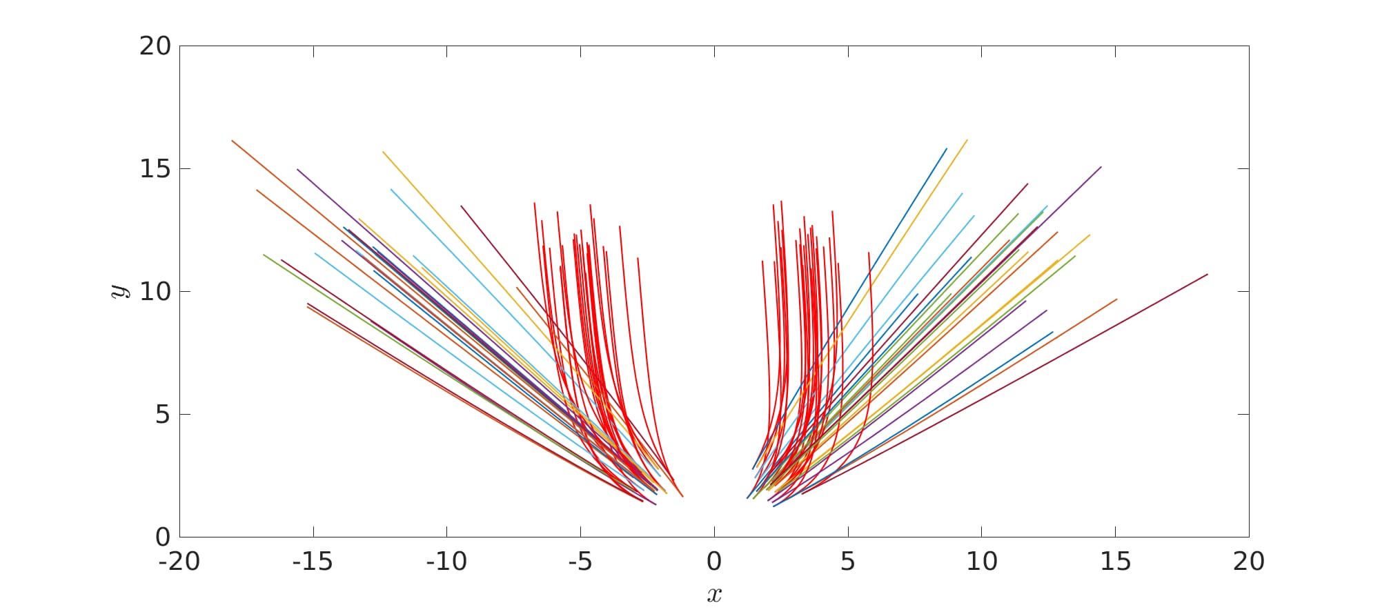
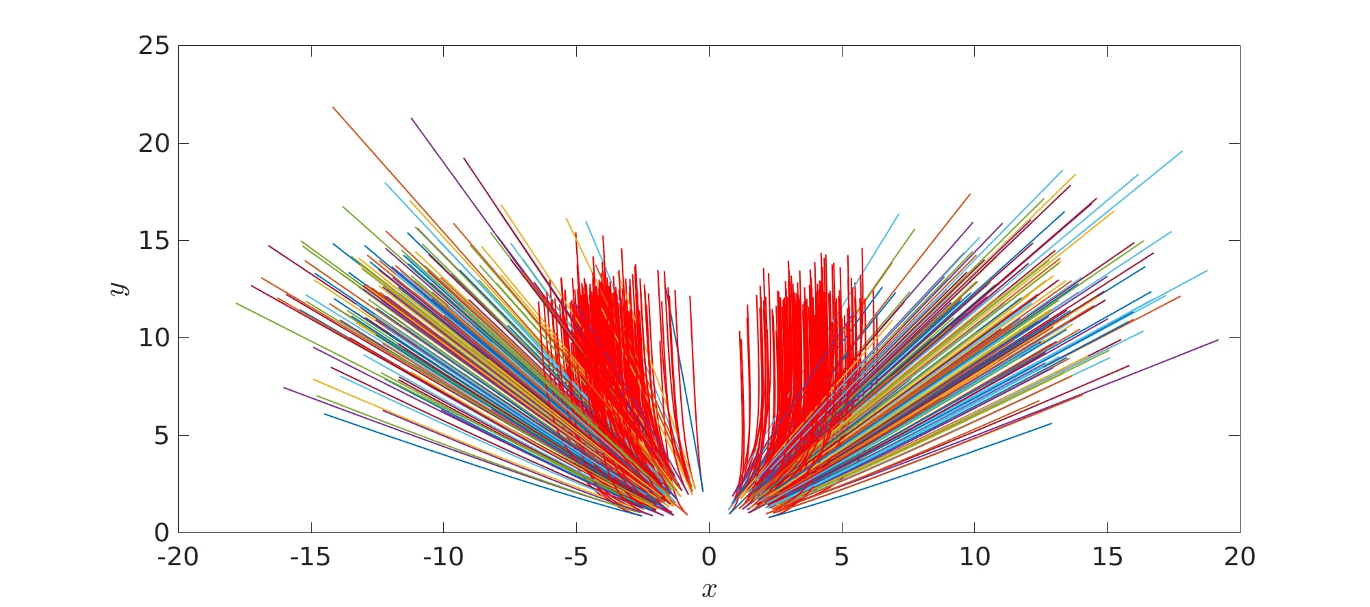
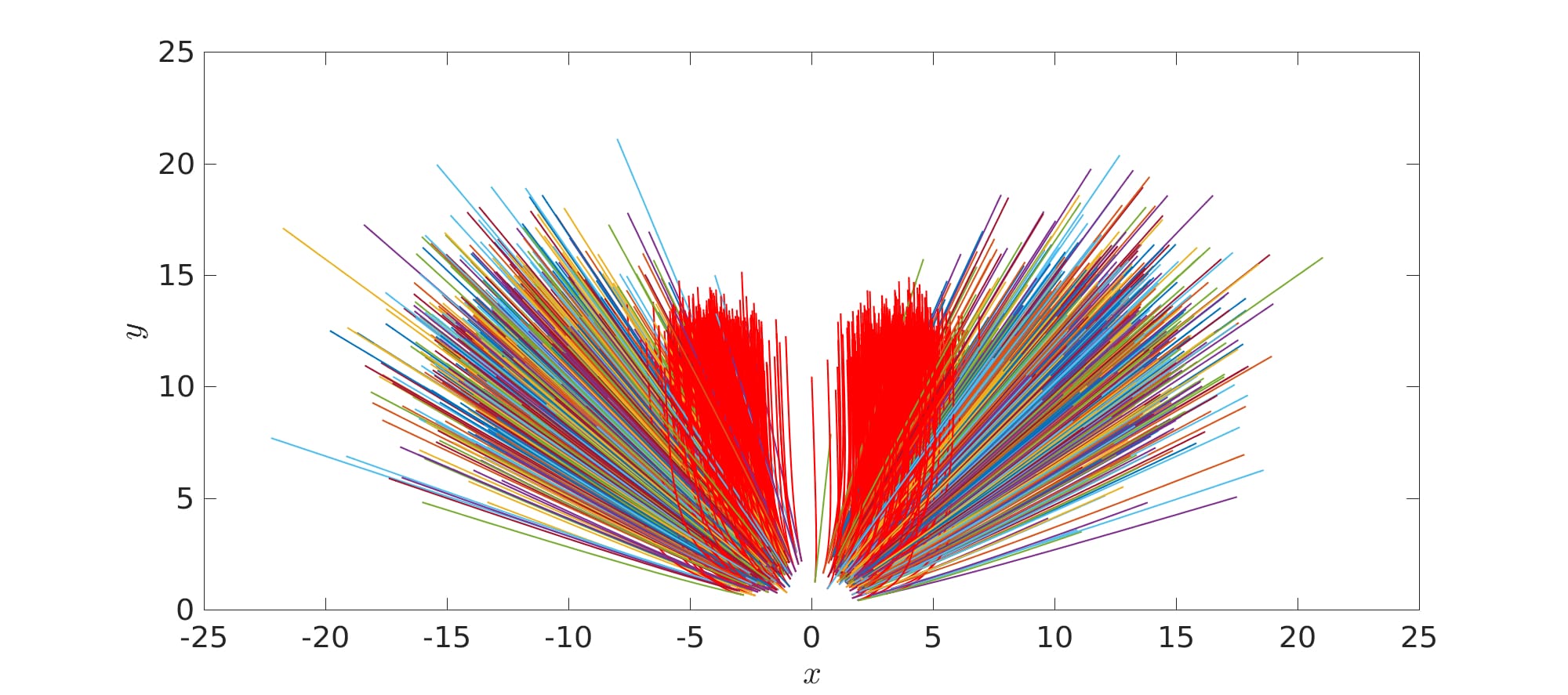
Figure 5.6: Free vs. optimally controlled (shown in red) dynamics. Top: $N=50$. Middle: $N=400$. Bottom: $N=2000$.

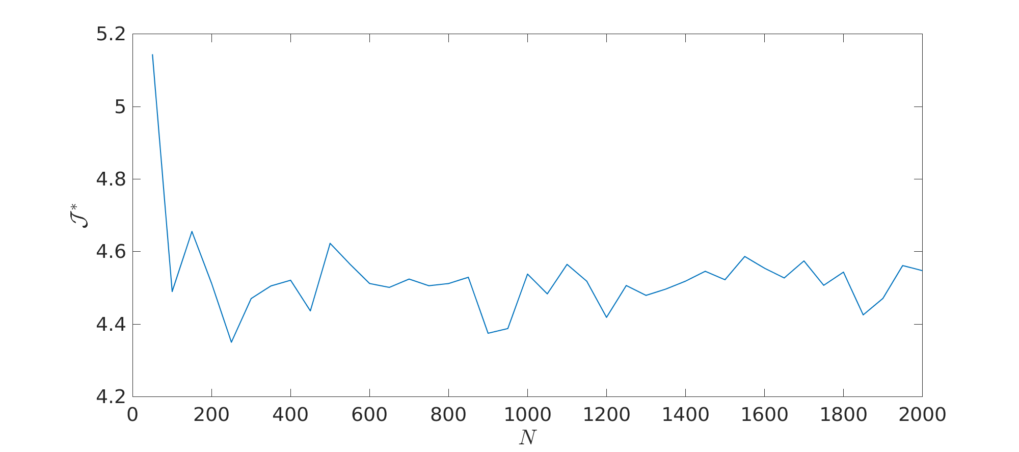
Figure 5.7: Evolution of $\mathcal{J}^{*}$ with $N\in\left\{50,100,\cdots,2000\right\}$.

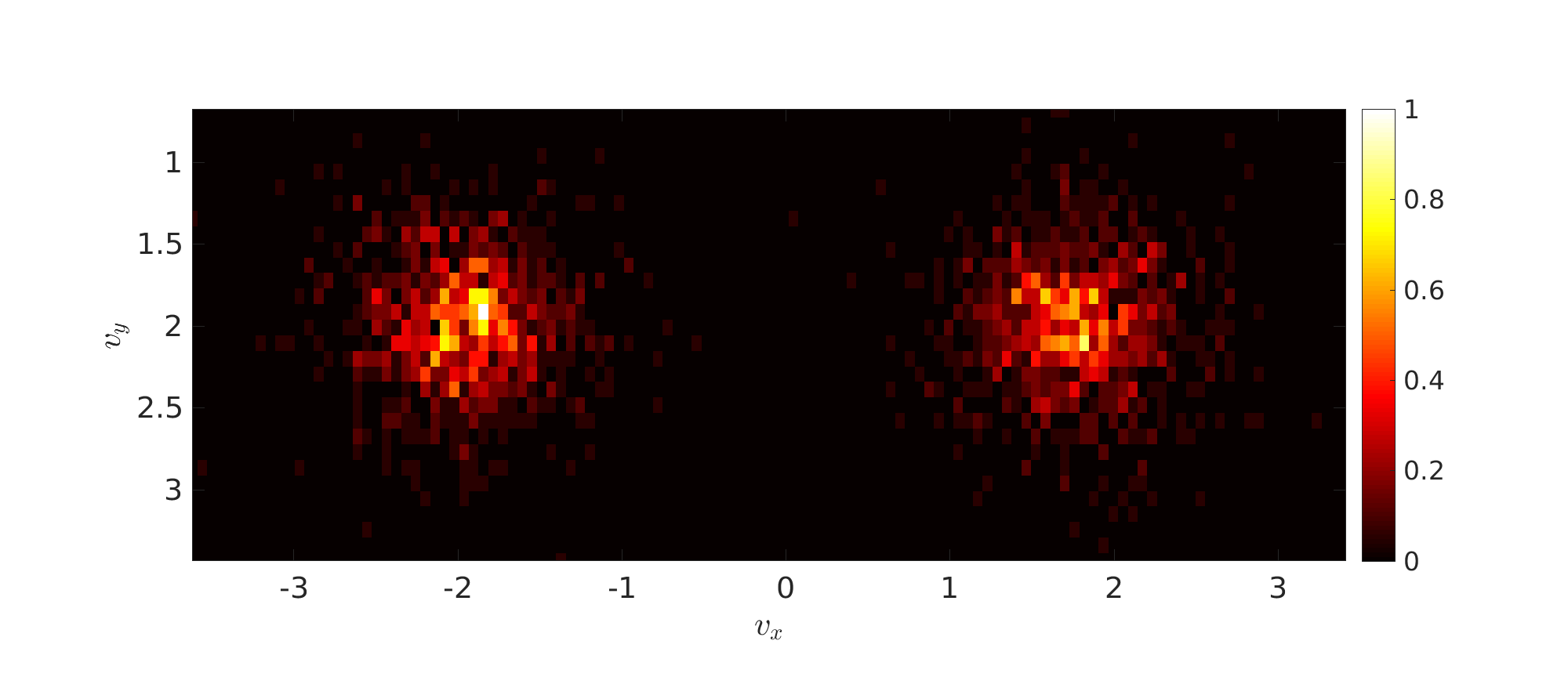
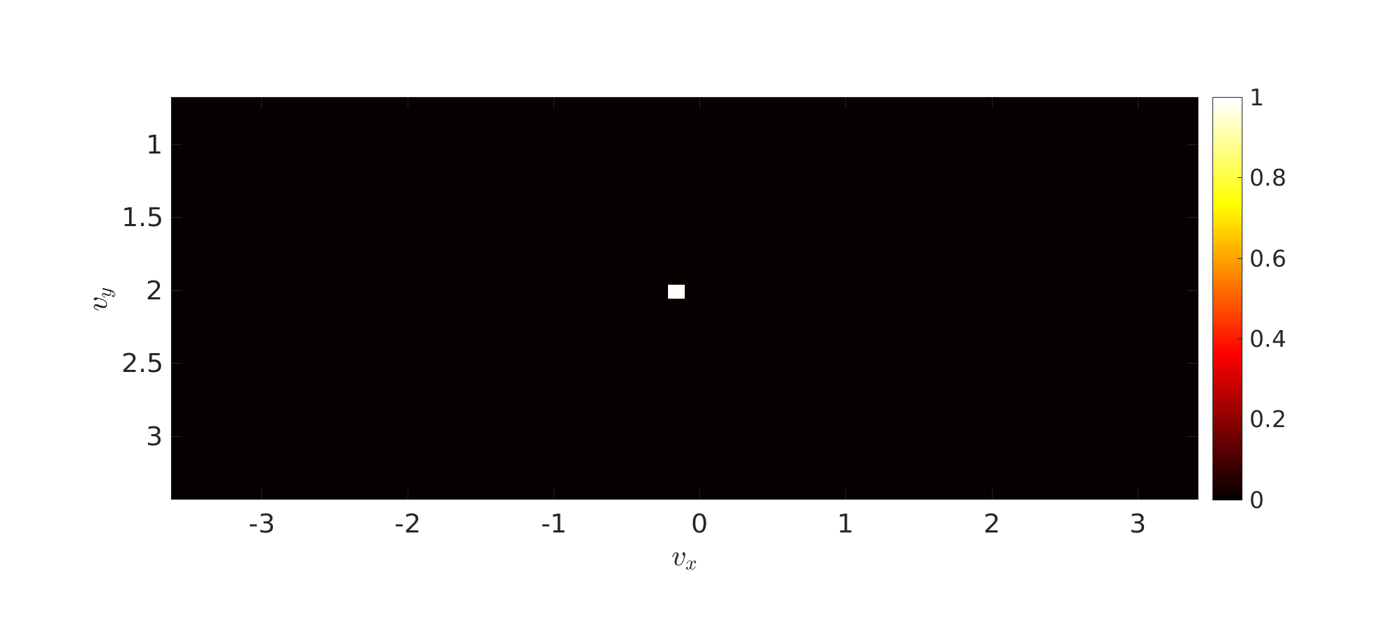
Figure 5.8: Marginal distributions of $f(T)$ on $v$, $N=2000$. Top: free setting. Bottom: controlled setting. Consensus emergence produces a concentration of the distribution around a single velocity close to $(0,2)$.

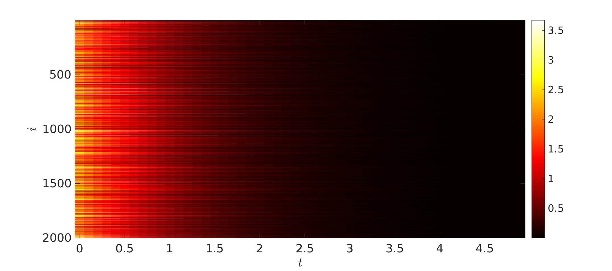
Figure 5.9: Heat map of $\left\|u_{i}^{*}(t)\right\|$ with $N=2000$.

Agents ($\mathbf{N}$)	50	100	150	200	250	300
Iterations ($\mathbf{I}$)	26	25	24	27	28	28
Time ($\mathbf{T}$)	0.1	0.1	0.3	0.7	1.1	1.4
$N$	1550	1600	1650	1700	1750	1800
$I$	28	28	28	28	28	28
$T$	49.1	51.7	52.8	58.8	59.8	65.0
$N$	1850	1900	1950	2000
$I$	27	29	28	28
$T$	65.4	75.3	77.4	82.8

Table 5.1: Number of iterations ($I$) and CPU time ($T$) in hours for $N$ agents for the discrete optimisation problem.

6 Acknowledgements

JAC was partially supported by the EPSRC grant EP/P031587/1.

References

- Albi et al. (2017a) Albi, G., Choi, Y.P., Fornasier, M., and Kalise, D. (2017a). Mean-field control hierarchy. Appl. Math. Optim., 76(1), 93–175.
- Albi et al. (2016) Albi, G., Bongini, M., Cristiani, E., and Kalise, D. (2016). Invisible control of self-organizing agents leaving unknown environments. SIAM J. Appl. Math., 76(3), 1683–1710.
- Albi et al. (2017b) Albi, G., Fornasier, M., and Kalise, D. (2017b). A Boltzmann approach to mean-field sparse feedback control. IFAC-PapersOnLine, 50(1), 2898 – 2903.
- Albi and Kalise (2018) Albi, G. and Kalise, D. (2018). (Sub) Optimal feedback control of mean field multi-population dynamics. Preprint, arXiv:1803.00301.
- Barzilai and Borwein (1988) Barzilai, J. and Borwein, J.M. (1988). Two-Point Step Size Gradient Methods. IMA J. Numer. Anal., 8(1), 141–148.
- Bongini and Fornasier (2014) Bongini, M. and Fornasier, M. (2014). Sparse stabilization of dynamical systems driven by attraction and avoidance forces. Netw. Heterog. Media, 9(1), 1–31.
- Bongini et al. (2015) Bongini, M., Fornasier, M., and Kalise, D. (2015). (Un)conditional consensus emergence under perturbed and decentralized feedback controls. Discrete Contin. Dyn. Syst. Ser. A, 35(9), 4071–4094.
- Bongini et al. (2017) Bongini, M., Fornasier, M., Rossi, F., and Solombrino, F. (2017). Mean-Field Pontryagin Maximum Principle. J. Opt. Theory Appl., 175(1), 1–38.
- Borzì and Schulz (2011) Borzì, A. and Schulz, V. (2011). Computational Optimization of Systems Governed by Partial Differential Equations. Society for Industrial and Applied Mathematics.
- Borzì and Wongkaew (2015) Borzì, A. and Wongkaew, S. (2015). Modeling and control through leadership of a refined flocking system. Math. Models Methods Appl. Sci., 25(2), 255–282.
- Caponigro et al. (2013) Caponigro, M., Fornasier, M., Piccoli, B., and Trélat, E. (2013). Sparse stabilization and optimal control of the Cucker-Smale model. Math. Control Relat. Fields, 3, 447–466.
- Carrillo et al. (2010a) Carrillo, J.A., Fornasier, M., Rosado, J., and Toscani, G. (2010a). Asymptotic flocking dynamics for the kinetic Cucker-Smale model. SIAM J. Math. Anal., 42, 218–236.
- Carrillo et al. (2010b) Carrillo, J.A., Fornasier, M., Toscani, G., and Vecil, F. (2010b). Particle, Kinetic, and Hydrodynamic Models of Swarming. In G. Naldi, L. Pareschi, and G. Toscani (eds.), Mathematical Modeling of Collective Behavior in Socio-Economic and Life Sciences, Series: Modelling and Simulation in Science and Technology, 297–336. Birkhäuser, Boston, MA.
- Cucker and Smale (2007) Cucker, F. and Smale, S. (2007). Emergent behavior in flocks. IEEE Trans. Automat. Control, 52(5), 852–862.
- Deroo et al. (2012) Deroo, F., Ulbrich, M., Anderson, B.D.O., and Hirche, S. (2012). Accelerated iterative distributed controller synthesis with a Barzilai-Borwein step size. In 2012 IEEE 51st IEEE Conference on Decision and Control (CDC), 4864–4870.
- Fornasier and Solombrino (2014) Fornasier, M. and Solombrino, F. (2014). Mean-field optimal control. ESAIM Control Optim. Calc. Var., 20(4), 1123–1152.
- Ha et al. (2010) Ha, S.Y., Ha, T., and Kim, J.H. (2010). Emergent behavior of a Cucker-Smale type particle model with nonlinear velocity couplings. IEEE Trans. Automat. Control, 55(7), 1679–1683.
- Ha and Liu (2009) Ha, S.Y. and Liu, J.G. (2009). A simple proof of the Cucker-Smale flocking dynamics and mean-field limit. Commun. Math. Sci., 7(2), 297–325.
- Kalise et al. (2017) Kalise, D., Kunisch, K., and Rao, Z. (2017). Infinite horizon sparse optimal control. J. Opt. Theory Appl., 172(2), 481–517.
- Kennedy and Eberhart (1995) Kennedy, J. and Eberhart, R. (1995). Particle swarm optimization. In Proceedings IEEE International Conference on Neural Networks, volume 4, 1942–1948.
- Mayne et al. (2000) Mayne, D.Q., Rawlings, J.B., Rao, C.V., and Scokaert, P.O. (2000). Constrained model predictive control: Stability and optimality. Automatica, 36(6), 789–814.
- Perea et al. (2009) Perea, L., Gómez, G., and Elosegui, P. (2009). Extension of the Cucker-Smale control law to space flight formations. AIAA Journal of Guidance, Control, and Dynamics, 32, 527–537.
- Pontryagin et al. (1962) Pontryagin, L.S., Boltyanskii, V.G., Gamkrelidze, R.V., and Mishchenko, E.F. (1962). The mathematical theory of optimal processes. Interscience Publishers John Wiley & Sons, Inc. New York-London.
- Shi and Eberhart (1998) Shi, Y. and Eberhart, R. (1998). A modified particle swarm optimizer. In Proceedings IEEE World Congress on Computational Intelligence, 69–73.