Non-Radial Pulsations in Post-Outburst Novae

Abstract

After an optical peak, a classical or recurrent nova settles into a brief (days to years) period of quasi-stable thermonuclear burning in a compact configuration nearly at the white dwarf (WD) radius. During this time, the underlying WD becomes visible as a strong emitter of supersoft X-rays. Observations during this phase have revealed oscillations in the X-ray emission with periods on the order of tens of seconds. A proposed explanation for the source of these oscillations are internal gravity waves excited by nuclear reactions at the base of the hydrogen-burning layer. In this work, we present the first models exhibiting unstable surface $g$-modes with periods similar to oscillation periods found in galactic novae. However, when comparing mode periods of our models to the observed oscillations of several novae, we find that the modes which are excited have periods shorter than that observed.

1 Introduction

A nova is an optical event caused by a thermonuclear runaway on the surface of a white dwarf (WD) (Gallagher & Starrfield, 1978). The thermonuclear runaway drives a rapid expansion of the WD where it shines brightly in the optical and loses much of its hydrogen-rich envelope via some combination of dynamical ejection, optically-thick winds, and/or binary interactions. Eventually enough mass is lost from the envelope so that the photospheric luminosity matches the nuclear burning luminosity and the WD radius recedes to a more compact configuration (Kato et al., 2014). Hydrogen burning does not cease, though, as a remnant envelope is slowly burned over days to decades. The hot and compact WD shines brightly in the UV and soft X-rays, appearing very similar to a persistent supersoft source (SSS) (Wolf et al., 2013). Dozens of SSSs from post-outburst novae are seen in M31 (Henze et al., 2010, 2011, 2014; Orio, 2006; Orio et al., 2010) and the Milky Way (Schwarz et al., 2011, and references therein) every year.

Many, if not all, SSSs exhibit periodic oscillations in their X-ray light curve with periods ($P_{\mathrm{osc}}$) in the range of 10-100 seconds, whose precise origin is unclear (Ness et al., 2015, and references therein). Odendaal et al. (2014) argue that in the case of Cal 83, its 67 s period could be the rotational period of the WD. Ness et al. (2015) point out that the observed drift of the precise $P_{\mathrm{osc}}$ of $\pm 3$ s can’t be easily explained by accretion spin-up or spin-down (due to high inertia of the WD) or by Doppler shifts of the emitting plasma due to the orbital motion. Furthermore, the $P_{\mathrm{osc}}=67$ s of Cal 83 is the longest in the known sample, so other WDs would need to be rotating even more rapidly. While the rotation rates of accreting WDs are still not well understood, spectroscopic measurements to date do not point to rapid rotation (Sion, 1999; Szkody et al., 2012; Kupfer et al., 2016).

Rotation is thus not a very promising mechanism for explaining these oscillations, though it cannot be ruled out until an independent determination of the WD rotation period is obtained in an oscillating SSS. A more promising explanation first proposed by Drake et al. (2003) is that the oscillations are caused by non-radial surface $g$-modes excited by the $\epsilon$-mechanism at the base of the hydrogen burning layer. However, the oscillations observed by Drake et al. (2003) for nova V1494 Aquilae were much longer. At $P_{\mathrm{osc}}\approx 2500$ s, these modes were more credibly explained as being driven by the $\kappa$-mechanism , where an ionization zone, rather than temperature-sensitive burning, is the source of an instability. Indeed, longer periods ($\sim 10-100$ minutes) have been observed in Cal 83 (Crampton et al., 1987; Schmidtke & Cowley, 2006) and nova V4743 Sgr (Ness et al., 2003), all consistent with oscilations most similar to GW Vir, driven by the ionized carbon and oxygen. These longer-period oscillations are not the focus of this work.

The expected $P_{\mathrm{osc}}$ for $\epsilon$-mechanism-driven $g$-modes was estimated in Ness et al. (2015) for a typical WD mass, envelope mass, and a constant-flux radiative envelope to be on the order of 10 s, in great agreement with the observed periods. Their calculation, however, could not assess whether the mode would grow unstably or damp out.

The configuration of a thin hydrogen-burning radiative envelope on a WD is similar to early planetary nebulae nuclei, as explored by Kawaler (1988). With a detailed non-adiabatic pulsational analysis, Kawaler (1988) found that $g$-modes were indeed excited by the $\epsilon$-mechanism. In a 0.618 $M_{\odot}$ planetary nebula nucleus model, higher-order modes with $P_{\mathrm{osc}}\approx 200\ \mathrm{s}$ were excited first when the luminosity was around $\log L/L_{\odot}\approx 3.1$, and lower order modes with $P_{\mathrm{osc}}\approx 70\ \mathrm{s}$ only being excited after the luminosity dropped to $\log L/L_{\odot}\approx 2.6$.

Encouraged by the promising results of Kawaler (1988) and Ness et al. (2015), we present in this paper the first detailed non-adiabatic calculations of the unstable modes in post-outburst nova models using the open source stellar evolution code MESA star (rev. 9575; Paxton et al., 2011, 2013, 2015) and the accompanying non-adiabatic stellar pulsation tool GYRE (Townsend & Teitler, 2013; Townsend et al., 2017). In §2 we explain the simulation details to obtain post-outburst nova models from MESA star for input into GYRE. Then in §3 we discuss mode propagation in our models and compare to previous simulations of oscillations in a planetary nebula nucleus. In §4, we present the periods and growth timescales of the modes calculated by GYRE from the nova models. We comment on how these modes compare to observed oscillation periods in §5 before summarizing in §6.

2 Stellar Models

To generate models for use in pulsational analysis, we use the MESA star code. Specifically, we use an inlist based on the nova test case scenario, which in turn was based off of the nova calculations of Wolf et al. (2013). In these models, hydrogen-rich material is accreted at a rate of $10^{-9}~{}M_{\odot}~{}\mathrm{yr^{-1}}$, which is a typical rate expected for cataclysmic variables (Townsley & Bildsten, 2005). Mass loss was handled by the built-in super-Eddington wind scheme described in Denissenkov et al. (2013) and Wolf et al. (2013), as well as a modified version of the built-in Roche lobe overflow mass loss scheme.

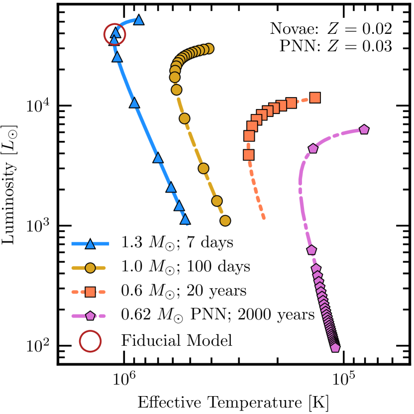
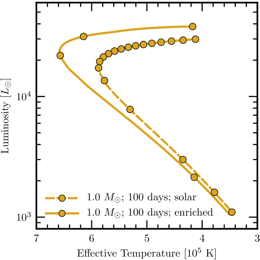
Figure 1: Evolution of all stellar models through the HR diagram. Different markers separate equal times of evolution. For example, between two yellow circles, 100 days have elapsed. Left: The three nova models that accrete solar composition material from the end of mass loss until their luminosities reach $10^{3}~{}L_{\odot}$. Also shown is the $M=0.6172~{}M_{\odot}$ planetary nebula nucleus introduced in Section 3. The maroon circle indicates a fiducial model of the 1.3 $M_{\odot}$ nova that we use as an example later in the paper. Right: Comparison between the $1.0~{}M_{\odot}$ nova models accreting solar composition and 25% core composition, 75% solar composition material. Again, markers along each track mark intervals of equal time.

The precise nature of the mass loss is not important because mass is lost in some form until the hydrogen rich layer is reduced to the maximum mass that can sustain steady hydrogen burning in a compact form, which is a function primarily of the WD mass. At this point the WD shrinks and enters its post-outburst phase, as found by Wolf et al. (2013); Kato et al. (2014). The precise nature of the mass loss greatly affects properties of the nova at the time of optical peak, which we are not interested in. However, extra mass loss in excess of that required to reduce the hydrogen layer mass down to a stable burning mass can truncate the duration of the post-outburst phase. To create the most favorable conditions for mode excitation, we shut off mass loss or gain once the WD shrinks to radii similar to the reddest steady-state burners found by Wolf et al. (2013). In general, super Eddington winds dominate mass loss for novae on higher-mass WDs, and Roche lobe overflow dominates mass loss for novae on the lowest-mass WD.

These models are non-rotating, though rotationally-induced instabilities can be responsible for mixing between core and accreted material (MacDonald, 1983; Livio & Truran, 1987; Sparks & Kutter, 1987). Rotation may also affect the stability and structure of $g$-modes in a stellar model, so we discuss the effects of modest rotation on the expected modes in §4. No diffusion is allowed, though at this high of an accretion rate, its effects on metal enrichment of the thermonuclear runaway would not be very pronounced (Iben et al., 1992; Prialnik & Kovetz, 1995; Yaron et al., 2005). Finally, we do not allow for any turbulent mixing at convective boundaries (i.e. undershoot/overshoot) during the thermonuclear runaway, which would also act to enhance the ejecta with metals (Casanova et al., 2010, 2011a, 2011b; Glasner et al., 2012). Mixing due to rotational instabilities, diffusion, and/or convective boundary mixing are all causes of the metal enhancement of nova ejecta indicated by optical and UV spectra (Gehrz et al., 1998; Downen et al., 2013) as well as evidence for dust formation (Geisel et al., 1970; Ney & Hatfield, 1978; Gehrz et al., 1980).

Rather than considering how exactly to parameterize and combine the mixing effects of rotational, diffusion-induced, and turbulent instabilities, we instead include a model where the accreted material is 25 percent core material, where “core composition” is defined as the composition sampled where the helium mass fraction first drops below one percent. The remaining 75 percent of accreted material is solar composition.

All inlists, models, and additional code used to produce these models will be posted on the MESA users’ repository, mesastar.org.

In total, four models were calculated: pure solar material accretion models for WD masses of 0.6 $M_{\odot}$, 1.0 $M_{\odot}$, and 1.3 $M_{\odot}$ and a metal-enriched accretion model for a 1.0 $M_{\odot}$ WD. The starting models were the endpoints of the similar nova simulations carried out by Wolf et al. (2013). The solar composition models were evolved through 2-3 nova cycles to erase initial conditions, while the metal-rich models were evolved through several flashes at an intermediate metallicity before being exposed to 25% enrichment to ease the transition. In all cases, model snapshots at every timestep after the end of mass loss to the end of the SSS phase were saved and form the basis for the analysis in the rest of this work.

Figure 1 shows the evolution of these nova models as well as a planetary nebula nucleus model with $M=0.617~{}M_{\odot}$ introduced in §3 through the HR diagram. The general trends are that higher mass WDs and more metal-rich accretion give faster, bluer, and more luminous evolution. Note that the markers break the evolution into stretches of equal duration, but the actual timesteps taken in the evolution were much shorter, taking somewhere between 30 and 60 timesteps to get through the SSS phase. Also indicated in Figure 1 is the location of a fiducial model from the $1.3~{}M_{\odot}$ simulation. We will refer to this model in subsequent sections as an example case for mode analysis.

3 Non-Radial Pulsation Analysis

With model snapshots of each of the novae throughout the SSS phase, we can use GYRE to determine their oscillation modes, focusing only on the $\ell=1$ (dipole) modes. We begin by looking at the adiabatic properties of our fiducial model before delving into non-adiabatic analyses.

3.1 Adiabatic Pulsation

GYRE analyzes a stellar model to find its radial and non-radial pulsation modes. While a non-adiabatic calculation is required to determine which of these modes are excited in a given stellar model, we can learn a lot from simpler adiabatic calculations to see what modes are available for excitation.

We aim to explain the observed oscillations as $g$-modes in the outer atmosphere, so some $g$-modes in our model must “live” in the outermost parts of our model. The upper panel of Figure 2 shows a propagation diagram of our fiducial 1.3 $M_{\odot}$ model during its SSS phase. Also indicated is the region of strong hydrogen burning, where we expect mode driving to occur.

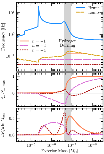
Figure 2: Profiles of the fiducial 1.3 $M_{\odot}$ model introduced in Figure 1. Top panel: Propagation diagram for our fiducial 1.3 $M_{\odot}$ post-outburst nova model in its outermost $10^{-4}~{}M_{\odot}$. The shaded region indicates the region over which 80% of the stellar luminosity is generated by CNO burning. Regions where the $n=-1,-2$ and $-4$ modes can propagate are plotted as horizontal lines at their respective frequencies. Middle panel: Eigenfunctions for the same three modes. Horizontal displacement dominates over radial displacement for these modes, so only the horizontal displacement is shown, normalized to a maximum of unity. Bottom panel: Mode inertia of these same modes expressed as $dE/d\ln M_{\mathrm{ext}}$, the derivative of the inertia with respect to $\ln[M(R)-M(r)]=\ln M_{\mathrm{ext}}$ so that equal areas under the curve indicate equal mode inertias. This is again normalized to integrate to unity.

After using GYRE to search for the eigenmodes of this model, we indeed find $g$-modes that live in the outer atmosphere with periods on the order of a few to tens of seconds. Horizontal displacement eigenfunctions for the $g$-modes with radial orders $n=-1,-2$, and $-4$ (in the Eckart-Osaki-Scuflaire classification scheme, as modified by Takata (2006)) are shown in the middle panel of Figure 2. The frequencies of these modes are also shown as horizontal lines spanning their allowed propagation regions (where their frequencies lie below both the Lamb and Brunt-Väisälä frequencies) in the upper panel. The bottom panel shows the distribution of inertia in these modes (normalized to integrate to unity), confirming that the modes indeed exist only within their allowed propagation regions. We see that the lowest order mode lives mostly in the burning region and the lower-density region above it. This makes this mode comparatively easier to excite than the other two, which have much of their energy in the higher-density helium-rich region below.

These are merely the modes in which the star is able to pulsate. To excite one, a driving force must do work on the mode, and a non-adiabatic caluclation is required to find such unstable modes. We discuss the relevant driving force and our non-adiabatic calculations next.

3.2 Non-adiabatic Pulsations and the $\epsilon$-Mechanism

The driving force relevant to novae in the SSS phase as well as planetary nebula nuclei is the $\epsilon$-mechanism. In the $\epsilon$-mechanism, the nuclear energy generation rate per unit mass $\epsilon$ is enhanced during a compression and attenuated during rarefaction. In this way, heat is added near the maximum temperatre of the cycle and removed near the minimum temperature, creating a heat engine that converts thermal energy into work (Eddington, 1926).

This phenomenon requires temperature sensitivity to produce feedback between the pulsation and $\epsilon$. For temperatures of interest to this work ($T\lesssim 10^{8}$ K), the CNO cycle is not yet beta-limited, and we still have $\epsilon\propto T^{9-14}$, so the $\epsilon$-mechanism can still be relevant.

There is, however, a minor complication. With periods on the order of tens of seconds, oscillations in temperature and density occur on the same timescales as the lifetimes of isotopes in the CNO cycle (Kawaler, 1988). This leads to lags between the phases of maximum temperature/density and the phase of maximum energy generation. As a result, the temperature and density sensitivities of the nuclear energy generation rate will differ from those in a non-oscillating system at the same average temperature and pressure.

The method for computing corrected partial derivatives of the energy generation rate were presented in Kawaler (1988), but since that work examined oscillations in a planetary nebula nucleus, which burns at a lower temperature than our nova models, an assumption in that work does not apply here. The details of how we calculate the partial derivatives and include them in GYRE are in Appendix A.

A mode is excited when a driving mechanism does enough work on the mode to exceed the energy lost through damping mechanisms over one oscillation cycle Unno et al. (1989, chapter V). In Figure 3, we show the cumulative work done on the $n=-1$ and $n=-2$ modes in our fiducial model. We show both the total cumulative work and only the work done by the $\epsilon$-mechanism. A net positive work indicates global mode driving and a net negative work indicates global mode damping. Note that in both cases, the contribution from the $\epsilon$-mechanism is positive, so it is always a driving force. However, in the $n=-2$ mode, nuclear driving is not strong enough to overcome other damping forces and the mode is globally damped. In the $n=-1$ mode, though, driving forces win and the mode is excited.

Notably, the total work done on the $n=-1$ mode exceeds that done by nuclear driving alone, which means another mechanism is also contributing to the instability. This mechanism is related to the steep luminosity gradient present in the burning region (i.e. not the $\kappa$-mechanism). We defer more exploration of this mechanism to subsequent work.

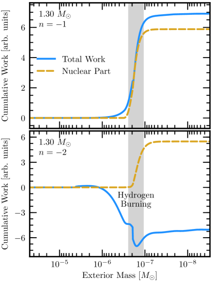
Figure 3: The cumulative integrated work done on the $n=-1$ (top panel) and $n=-2$ (bottom panel) modes in the fiducial model in arbitrary units as a function of the exterior mass $\Delta M_{\mathrm{ext}}(r)=m(R)-m(r)$. The solid blue line is the result of a fully nonadiabatic calculation, with the broken gold line being the contribution from the $\epsilon$-mechanism. The net positive work done in the top panel indicates that the $n=-1$ mode is unstable, while the net negative work in the bottom panel indicates that the $n=-2$ mode is stable despite the destabilizing (positive) contribution of the $\epsilon$ term.

Before looking further at the modes excited in the nova models, we first analyze a planetary nebula nucleus model similar to that of Kawaler (1988) to verify that we obtain a similar set of excited modes.

3.3 Planetary Nebula Nucleus

The planetary nebula nucleus (PNN) model from Kawaler (1988) was created by first evolving a star with a ZAMS mass of a 3.0 $M_{\odot}$ star with a metallicity of $Z=0.03$ to the AGB and then stripping its envelope gradually away.

The MESA test suite includes a test case, make_co_wd, which evolves a star to the AGB and through one thermal pulse from the helium burning shell, and then greatly increases the efficiency of AGB winds to reveal the WD. We used this test case as a basis and changed three controls to create our PNN model. First, we set the metallicity to 0.03 instead of the test case’s default value of 0.02. Secondly, we evolve the model from the pre-main sequence (rather than interpolating from a default suite of models) due to the specific metallicity. Finally, we adusted the initial mass to $3.30~{}M_{\odot}$ so that the final mass of $M=0.6172~{}M_{\odot}$) closely resembled the mass of the PNN in Kawaler (1988) of $M=0.6185~{}M_{\odot}$.

Once the model reached an effective temperature greater than 10,000 K, we changed its nuclear network to match the network used in the nova simulations (cno_extras.net). At $T_{\mathrm{eff}}=60,000$ K, we halted the enhanced mass loss that accelerated the thermal pulse phase in order to resume normal PNN evolution. We then saved profiles for pulsational analysis at every timestep once the effective temperature exceeded 80,000 K, and we halted evolution when the luminosity dropped below 100 $L_{\odot}$.

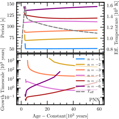
Figure 4: Evolution of $\ell=1$ $g$-modes in the planetary nebula nucleus model through the depletion of its hydrogen envelope. The top panel shows how the periods of the six lowest-order $g$-modes change in time. The effective temperature is also shown for comparison to evolution in the HR diagram. The bottom panel shows the evolution of the growth timescale for each mode if it is unstable.

The evolution of the model’s $g$-mode properties through its PNN phase is shown in Figure 4 for six lowest-order modes. The first mode to be excited was a $g$-mode with radial order $n=-6$. The period of this mode stayed consistently near 150 s and its growth time stayed in the range of hundreds to thousands of years (still shorter than the hydrogen-burning lifetime of the PNN). The period agrees well with the $k=6$ column of Table 3 in Kawaler (1988), but we find growth timescales that are longer by one or more orders of magnitude with the mode being stabilized sooner than in Kawaler (1988).

Other modes have matching or very nearly matching periods, but the growth times we find are typically much longer than those of Kawaler (1988). In addition to the modes shown in Figure 4, we see the $n=-7$ and $n=-8$ modes excited, but not the $n=-9$ mode as in Kawaler (1988), consistent with the general trend of higher stability in our models.

We searched for modes both while accounting for the phase lags in the energy generation rate and while not accounting for them. In both PNN and nova models, adding in the effects of phase lags increases growth times and stabilizes modes that would otherwise be unstable. This is because the phase of peak heat injection is moved away from the phase of peak temperature/density, weakening the heat engine set up by the $\epsilon$-mechanism.

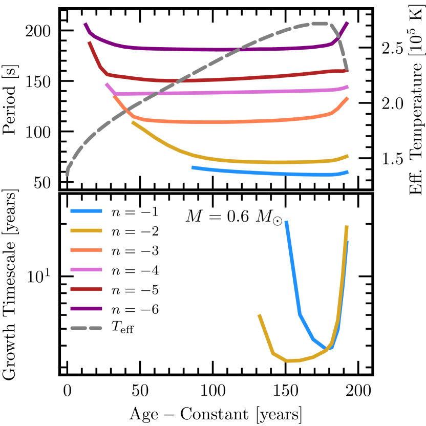
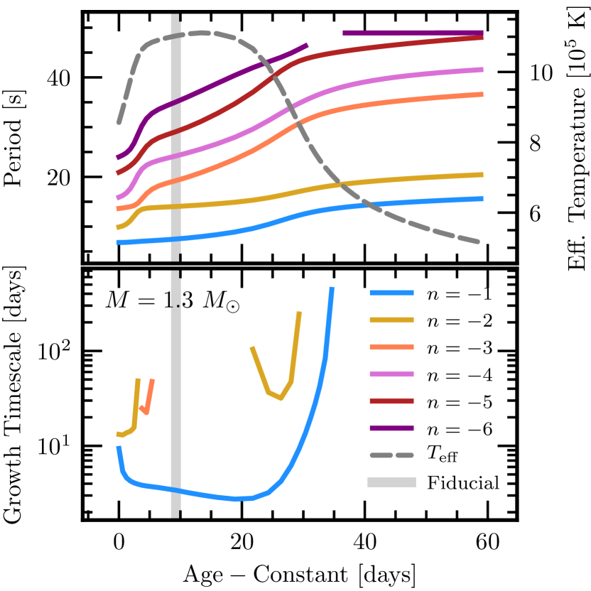
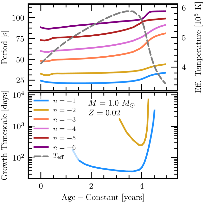
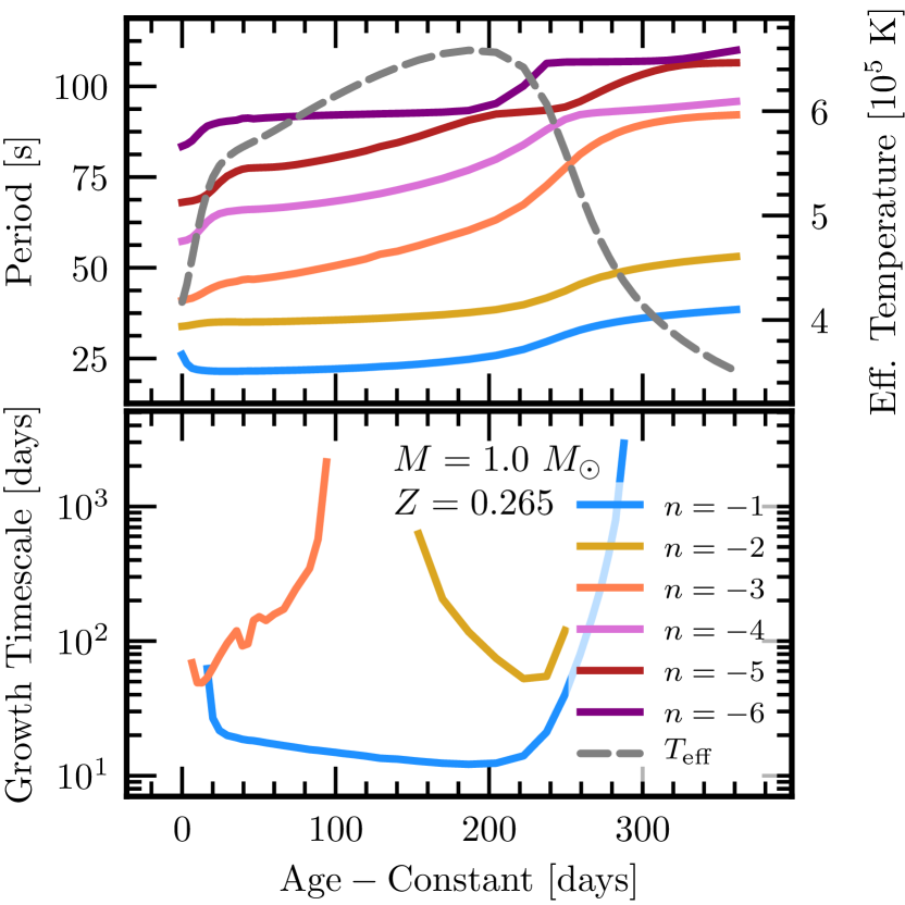
Figure 5: Evolution of the $\ell=1$ $g$-modes modes of each post-outburst nova model (masses and compositions indicated in each plot). Similar to Figure 4, the top panels show mode periods and effective temperatures while the bottom panels show growth timescales. Points in a top panel represent unstable modes only if an accompanying point at the same age and mode order appears in the lower panel. A gray vertical band in the $1.3~{}M_{\odot}$ plot indicates from where the fiducial model referenced elsewhere in this work is taken.

4 Supersoft Nova Modes

Figure 5 shows the evolution of the periods of low-order $g$-modes in the post-outburst nova models as well as the evolution of these modes’ growth timescales. The effective temperature evolution is also shown in these figures, revealing that the most rapid excitation occurs in the approach to the peak effective temperature at the ”knee” of the HR diagram shown in Figure 1.

We find unstable modes excited on timescales shorter than the supersoft phase lifetime in all four nova models. Excited modes had periods as short as 7 seconds in the $1.3~{}M_{\odot}$ model and as long as 80 seconds for the $0.6~{}M_{\odot}$ model. Unlike the PNN model, only lower-order modes were excited. The $n=-1$ and $n=-2$ modes are excited at some point in every model, while the $n=-3$ mode is excited in the $1.3~{}M_{\odot}$ and enriched $1.0~{}M_{\odot}$ models only. In the $1.0~{}M_{\odot}$ and $1.3~{}M_{\odot}$ models, only the $n=-1$ mode exhibits short enough growth timescales for the mode to grow by several $e$-foldings before it is stabilized, but the $0.6~{}M_{\odot}$ model actually excites its $n=-2$ mode earlier and more rapidly than the $n=-1$ mode.

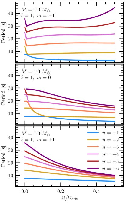
Figure 6: Dependence of the mode periods on the rotation rate as a fraction of the critical rotation rate for the $m=-1$ (top), $m=0$ (middle), and $m=+1$ (bottom) modes in our $1.3~{}M_{\odot}$ fiducial model. At any given rotation rate, the mode with a period of 8–9 seconds is excited with a growth timescale of around 2.5 days. For the $m=+1$ case, this is always the $n=-1$ mode, but due to avoided crossings, the excited mode switches to the $n=-2$ mode in the $m=-1$ and $m=0$ cases at a modest fraction of the critical rotation frequency. No other modes are ever excited on timescales shorter than or comparable to the SSS lifetime.

The general trend is that more massive WDs exhibit shorter periods and shorter growth times. We find that metal enrichment has little effect on the mode periods, but it significantly reduces growth timescales and the duration of the SSS phase.

The models made in MESA star are non-rotating, but we can probe the effects of rotation on the mode periods and growth timescales by using the traditional approximation (Bildsten et al., 1996; Townsend, 2005).

We investigated how the periods and growth times for $\ell=1$ modes changed in response to varying the rotation rate $\Omega$ in our fiducial 1.3 $M_{\odot}$ model. Figure 6 shows how periods of $\ell=1$ modes are affected by rotation up to an $\Omega$ of half of the critical rotation rate $\Omega_{\mathrm{crit}}=\sqrt{8GM/(27R^{3})}\approx 1\,\textrm{Hz}$. We now summarize the results.

Higher-order zonal ($m=0$) and prograde ($m=1$) modes’ periods decreased modestly with increasing $\Omega$, but for higher-order retrograde ($m=-1$) modes, periods increased modestly after an initial drop due to a series of avoided crossings. However, across all $\Omega$’s, there was only ever one mode excited on timescales comparable to or shorter than the nova evolution timescale. The period of this mode is 8–9 seconds and its growth timescale is 2.5 days, in great agreement with the non-rotating results shown in Figure 5. Due to the avoided crossings, this mode changes in radial order from $n=-1$ to $n=-2$ at about 2% and 12% of $\Omega_{\mathrm{crit}}$ for the $m=-1$ and $m=0$ cases, respectively. With no significant change in the periods of the excited mode, we expect no observable effect from rotation on these oscillations other than incidental effects rotation may have on the accretion and runaway processes.

5 Comparison to Observation

The goal of this work was to explain the oscillations in post-outburst novae and persistent supersoft sources described in Ness et al. (2015) and references therein. We’ve demonstrated that the $\epsilon$-mechanism is indeed an effective means to excite $g$-modes with periods similar to those in observed SSSs.

However, we have only demonstrated that these modes are unstable in the linear regime. We cannot predict amplitudes for these oscillations to construct a X-ray light curve for comparison. A more complex non-linear calculation would be required to make such a robust prediction.

Fortunately, our work has confirmed, as expected, that the periods are most sensitive to the mass of the underlying WD rather than composition or rotation. Thus, a nova with a known WD mass and observed oscillations would provide a means to check the efficacy of $g$-modes as a source for these oscillations. We now review the oscillating post-outburst novae presented in Ness et al. (2015) and compare them to our models.

5.1 RS Ophiuchi

RS Ophiuchi (RS Oph) is a recurrent nova with recurrence times as short as nine years. From spectral measurements, Brandi et al. (2009) find a best orbital solution for a WD with a mass in the range of $1.2-1.4~{}M_{\odot}$. From the recurrence time alone, models from Wolf et al. (2013) limit the WD mass to $M>1.1~{}M_{\odot}$, while the effective temperature and duration of the supersoft phase are most consistent with models with a mass near $1.3~{}M_{\odot}$.

However, according to Ness et al. (2015), RS Oph has oscillations with a period of 35 seconds, which is significantly longer than the $\approx 6-10$ second periods seen in the $n=-1$ mode of our $1.3~{}M_{\odot}$ model. Even giving a generously low mass of $1.0~{}M_{\odot}$ would require exciting the mode only at late times when it is already stabilizing or by tapping into the $n=-2$ mode during the brief duration that it is unstable.

5.2 KT Eridani

KT Eridani (KT Eri) is a nova that also exhibited oscillations with periods of roughly 35 s at multiple times in its supersoft evolution (Beardmore et al., 2010; Ness et al., 2015). Jurdana-Šepić et al. (2012) estimate from the supersoft turn-on time and possible presence of neon enrichment, the mass of the underlying white dwarf is $1.1~{}M_{\odot}\leq M_{\mathrm{WD}}\leq 1.3~{}M_{\odot}$. With a turn-off time of around 300 days (Schwarz et al., 2011), models from Wolf et al. (2013) are consistent with this contraint. Similar to RS Oph, the lowest order (and most easily excited) modes from the 1.0 and 1.3 $M_{\odot}$ models still cannot explain the observed oscillations, but second or third order modes are not out of the question if they could be excited.

5.3 V339 Delphini

V339 Delphini (V339 Del) is a nova with an observed 54 s oscillation (Beardmore et al., 2013; Ness et al., 2013). Shore et al. (2016) provide an estimate for the ejecta mass of V339 Del of $2-3\times 10^{-5}~{}M_{\odot}$. With this and its SSS turn-off time of 150-200 days, V339 Del is consistent with a WD mass of $M_{\mathrm{WD}}\approx 1.0-1.1~{}M_{\odot}$ (Wolf et al., 2013). Again returning to our $1.0~{}M_{\odot}$ models, we must rely on even higher order $n<-2$ to explain the observed oscillations. The $n=-3$ mode is unexcited in the solar composition model, and in the metal-enriched model, it is only marginally unstable in that its growth timescale is comparable to the duration in which it is unstable. Even then the $n=-3$ mode has a period that is slightly too short during this phase, but higher-order modes are never excited at all. It is difficult to explain the oscillations in V339 Del with our models.

5.4 LMC 2009a

LMC 2009a is a recurrent nova, having first been detected in outburst in 1971. From its recurrence time as well as the SSS duration and temperature of the 2009 outburst, Bode et al. (2016) estimate the mass of the underlying WD to be $M_{\mathrm{WD}}\approx 1.1~{}M_{\odot}-1.3~{}M_{\odot}$. The oscillations during the SSS phase reported in Ness et al. (2014, 2015); Bode et al. (2016) had a period of 33 seconds. With a similar period and mass estimate to KT Eri, the $g$-mode explanation of these oscillations is similarly tenuous.

Our models show that metal enrichment does not change mode periods substantially, and even relatively rapid rotation cannot greatly affect the periods of excited modes. Rather, it seems that without some more exotic physics that can couple to higher-order modes, the $g$-modes we see in our model cannot adequately explain the oscillations observed in the novae detailed in Ness et al. (2015).

6 Conclusions

We have used MESA models to confirm the earlier work of Kawaler (1988) on planetary nebula nuclei. We then extended that work to see what, if any, modes are excited in post-outburst novae via the $\epsilon$-mechanicsm. In all our models, we found unstable modes with growth timescales shorter than the lifetime of the post-outburst supersoft phase.

While metal-enhancement of the WD envelope did expedite the evolution through the post-outburst phase and the growth of any excited modes, it did not greatly influence the periods of these modes. Similarly, rotation only affected the periods of higher-order modes that were not excited, so it is unlikely to have a strong effect on any oscillations this mechanism might produce.

Finally, we compared our results to the observed oscillations of several novae. Broadly, the excited modes we find for comparable nova models have periods that are too short to explain the observed ocsillations, and neither metal enhancement nor rotation are sufficient to excite higher-order modes or increase an excited mode’s period.

Appendix A Calculation of Phase Lags

To calculate the sensitivity of the CNO burning rate to density and temperature perturbations, we followed the method of Kawaler (1988) with several changes. For completeness, we outline the entire calculation here.

Thermonuclear burning in the post-outburst nova is dominated by the CNO cycle. We consider only the basic CN cycle since it produces most of the energy. The reactions involved are

$${}^{12}\mathrm{C}+p \rightarrow{} {}^{13}\mathrm{N}+\gamma,$$ (A1)

$${}^{13}\mathrm{N} \rightarrow{} {}^{13}\mathrm{C}+e^{+}+\nu_{e},$$ (A2)

$${}^{13}\mathrm{C}+p \rightarrow{} {}^{14}\mathrm{N}+\gamma,$$ (A3)

$${}^{14}\mathrm{N}+p \rightarrow{} {}^{15}\mathrm{O}+\gamma,$$ (A4)

$${}^{15}\mathrm{O} \rightarrow{} {}^{15}\mathrm{N}+e^{+}+\nu_{e},$$ (A5)

$${}^{15}\mathrm{N}+p \rightarrow{} {}^{12}\mathrm{C}+\alpha.$$ (A6)

We will index the reactants of equations (A1)–(A6) as 1–6. That is, ${}^{12}\mathrm{C}$ will be denoted by the number 1 in subscripts and ${}^{15}\mathrm{N}$ by 6. These indices will be cyclic so that $1-1=6$ and $6+1=1$.

For an isotope $i$ that is both produced and destroyed via proton captures, the total number of ions of isotope $i$ is represented by $N_{i}$. Then the net rate of production of these isotopes is

$$\frac{DN_{i}}{Dt}=-N_{i}n_{p}\left\langle{}\sigma{}v\right\rangle{}_{i}+N_{i-1}n_{p}\left\langle{}\sigma{}v\right\rangle{}_{i-1},$$ (A7)

where $D/Dt$ is the Lagrangian time derivative, $n_{p}$ is the number density of protons, and the $\left\langle{}\sigma{}v\right\rangle{}$’s are the thermally-averaged reaction rates. If the isotope is created via a beta decay, the second term is replaced by $N_{i-1}\lambda_{i-1}$ where $\lambda_{i-1}$ is the decay rate of isotope $i-1$. Similarly, if the isotope is destroyed by a beta decay, then we replace the first term in (A7) with $-N_{i}\lambda_{i}$. The total number of ions of isotopes is related to its mass fraction $X_{i}$ and mass number $A_{i}$ via $N_{i}\propto X_{i}/A_{i}$. Thus we can rewrite (A7) in terms of the mass fraction via

$$\frac{DN_{i}}{Dt}\propto\frac{1}{A_{i}}\frac{DX_{i}}{dt}.$$ (A8)

For simplicity, we also introduce a generalized destruction rate, $K_{i}$ that is $\lambda_{i}$ for isotopes destroyed via beta decay and $n_{p}\left\langle{}\sigma{}v\right\rangle{}_{i}$ for those destroyed by proton captures. This gives a generalized rate equation of

$$\frac{DX_{i}}{Dt}=-X_{i}K_{i}+\frac{A_{i}}{A_{i-1}}X_{i-1}K_{i-1}.$$ (A9)

In the background equilibrium state, these rates all vanish once the mass fractions have settled to the preferred configuration. Now we introduce Lagrangian perturbations (denoted by the $\delta$ symbol) in temperature and density with frequency $\sigma$,

$$\rho\to\rho_{0}+\delta\rho\,e^{-i\sigma t}\qquad T\to T_{0}+\delta T\,e^{-i\sigma t},$$ (A10)

where subscripts of 0 indicate the constant equilibrium values. The generalized destruction rates, $K_{i}$ will also change, but only for reactions involving proton captures:

$$K_{i}=\lambda_{i}\to\lambda_{i,0}\qquad K_{i}=n_{p}\left\langle{}\sigma{}v\right\rangle{}_{i}\to K_{i,0}+K_{i,0}\left[\frac{\delta\rho}{\rho}+\nu_{i}\frac{\delta T}{T}\right]e^{-i\sigma t},$$ (A11)

where $\nu_{i}=d\ln\left\langle{}\sigma{}v\right\rangle{}_{i}/d\ln T$. Similarly, the mass fractions $X_{i}$ and their derivatives will also change:

$$X_{i}\to X_{i,0}+\delta X_{i}\,e^{-i\sigma t}\qquad\frac{DX_{i}}{Dt}\to-i\sigma\delta X_{i}\,e^{-i\sigma t}.$$ (A12)

Phase lags will only be present if the values of $\delta X_{i}$ are complex. Now applying the perturbations of (A11) and (A12) to (A9), subtracting off the equilibrium solution, and dividing out the exponential dependence gives

$$-i\sigma\delta X_{i}=-\left(\delta X_{i}K_{i,0}+X_{i,0}\delta K_{i}\right)+\frac{A_{i}}{A_{i-1}}\left(\delta X_{i-1}K_{i-1,0}+X_{i-1,0}\delta K_{i-1}\right),$$ (A13)

where we’ve left the perturbation of the generalized rate as a generic $\delta K_{i}$. Specializing to the three classes of isotopes (creation by beta decay, destruction by beta decay, or no beta decays) and noting that by conservation of mass,

$$\frac{A_{i}}{A_{i-1}}\left(\delta X_{i-1}K_{i-1,0}+X_{i-1,0}\delta K_{i-1}\right)=X_{i,0}K_{i,0}\left(\frac{\delta X_{i-1}}{X_{i-1,0}}+\frac{\delta K_{i-1}}{K_{i-1,0}}\right),$$ (A14)

we get

$$i\frac{\sigma}{K_{i,0}}\frac{\delta X_{i}}{X_{i,0}} = \left(\frac{\delta X_{i}}{X_{i,0}}+\frac{\delta K_{i}}{K_{i,0}}\right)-\left(\frac{\delta X_{i-1}}{X_{i-1,0}}+\frac{\delta K_{i-1}}{K_{i-1,0}}\right),$$ (A15)

$$\frac{K_{i,0}-i\sigma}{K_{i,0}}\frac{\delta X_{i}}{X_{i,0}}-\frac{\delta X_{i-1}}{X_{i-1,0}} = \frac{\delta K_{i-1}}{K_{i-1,0}}-\frac{\delta K_{i}}{K_{i,0}},$$ (A16)

$$\frac{K_{i,0}-i\sigma}{K_{i,0}}\frac{\delta X_{i}}{X_{i,0}}-\frac{\delta X_{i-1}}{X_{i-1,0}} = (\nu_{i-1}-\nu_{i})\frac{\delta T}{T_{0}}\qquad(i=1,4),$$ (A17)

$$\frac{\lambda_{i}-i\sigma}{\lambda_{i}}\frac{\delta X_{i}}{X_{i,0}}-\frac{\delta X_{i-1}}{X_{i-1,0}} = \frac{\delta\rho}{\rho_{0}}+\nu_{i-1}\frac{\delta T}{T_{0}}\qquad(i=2,5),$$ (A18)

$$\frac{K_{i,0}-i\sigma}{K_{i,0}}\frac{\delta X_{i}}{X_{i,0}}-\frac{\delta X_{i-1}}{X_{i-1,0}} = -\frac{\delta\rho}{\rho_{0}}-\nu_{i}\frac{\delta T}{T_{0}}\qquad(i=3,6).$$ (A19)

Here (A16) is still a general result while (A17) - (A19) relate the relative mass fraction perturbations to the equilibrium conditions and the temperature and density perturbations for isotopes that are created and destroyed by proton captures (A17), created by proton captures and destroyed by beta decays (A18), and created by beta decays and destroyed by proton captures (A19). These constitute a set of six equations in six unknowns. For a given temperature, density, and equilibrium set of abundances, we can then query the rates module of MESA to get $\lambda_{i}$, $K_{i,0}(\rho_{0},T_{0})$, and $\nu_{i}(T_{0})$ to get an expression for $\delta X_{i}$ in terms of $\sigma$, $\delta T/T_{0}$, and $\delta\rho/\rho_{0}$. In general, this has the form

$$\frac{\delta X_{i}}{X_{i,0}}=\left(\alpha\frac{\delta\rho}{\rho_{0}}+\beta\frac{\delta T}{T_{0}}\right)e^{-i\sigma t},$$ (A20)

where the $\alpha$’s and $\beta$’s come from solving the system of equations above. They depend only on the various $K_{i}$’s, $\nu_{i}$’s, and $\sigma$. They are in general complex, giving rise to phase delays between the temperature/density perturbation and the actual changes in abundances. Kawaler (1988) solved for these $\alpha$’s and $\beta$’s explicitly in the limit where beta decays occur much more quickly than proton captures. This limit is valid in the case of a PNN, but at the higher temperatures present in some of the post-outburst novae, this assumption fails, so the full matrix inversion calculation is needed to solve for these quantities.

To see how this affects wave excitation via the $\epsilon$-mechanism, we need to relate these $\alpha$’s and $\beta$’s to the nuclear energy generation rate. The energy generation rate due to the destruction of species $i$ is given by

$$\epsilon_{i}=\frac{X_{i}K_{i}Q_{i}}{A_{i}m_{p}},$$ (A21)

where $K_{i}$ is again the generalized destruction rate and $Q_{i}$ is the energy released by the destruction of one isotope (roughly the difference in binding energies). Then the total energy generation rate is just the sum over all of these rates. After accounting for the perturbations in $K_{i}$ and $X_{i}$, the perturbation in the overall energy generation rate is

$$\frac{\delta\epsilon}{\epsilon_{0}}=\left(A\frac{\delta\rho}{\rho_{0}}+B\frac{\delta T}{T_{0}}\right)e^{-i\sigma t},$$ (A22)

where

$$A=\frac{d\ln\epsilon}{d\ln\rho}=\frac{\left(\sum_{i}\alpha_{i}\epsilon_{i}\right)+\epsilon_{1}+\epsilon_{3}+\epsilon_{4}+\epsilon_{6}}{\epsilon_{0}}$$ (A23)

and

$$B=\frac{d\ln\epsilon}{d\ln T}=\frac{\left(\sum_{i}\beta_{i}\epsilon_{i}\right)+\nu_{1}\epsilon_{1}+\nu_{3}\epsilon_{3}+\nu_{4}\epsilon_{4}+\nu_{6}\epsilon_{6}}{\epsilon_{0}}.$$ (A24)

In the long-period limit $\sigma\to 0$, we expect $A\to 1$, but in general, $A<1$ for periods in the 1-1000 second range. Similarly, $B$ is smaller than the expected unperturbed value for periods in this range, causing an enhanced stability in the burning rate with changes to temperature and densities.

As a simple check that our method is consistent with the work of Kawaler (1988), the left panel of Figure 7 reproduces Figure 3 of that paper, where the derivatives $A=d\ln\epsilon_{\mathrm{nuc}}/d\ln\rho$ and $B=d\ln\epsilon_{\mathrm{nuc}}/d\ln T$ are plotted for a particular temperature, density, and composition. We find excellent agreement with our general approach. The right panel of Figure 7 shows how the actual values of $A$ and $B$ vary as a function of period for our fiducial $1.3~{}M_{\odot}$ post-outburst nova model as well as a much hotter version of that model, demonstrating that temperature and density sensitivity indeed vanish at such high temperatures as the reaction cycle becomes limited by beta decays.

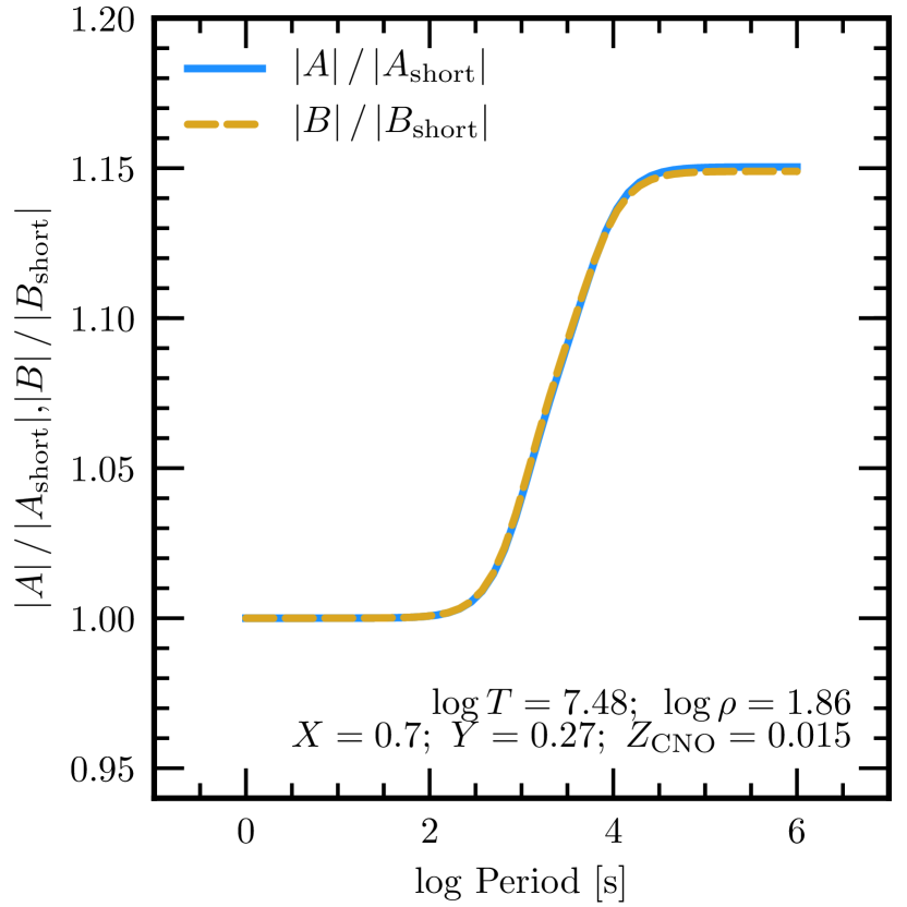
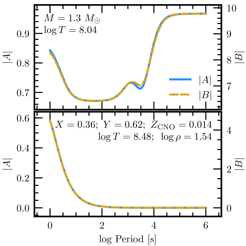
Figure 7: Left: dependence of the logarithmic derivatives of the nuclear energy generation rate (relative to the short-period limit) on pulsation period. This figure corroborates the similar Figure 3 from Kawaler (1988). Right: the actual values of these derivatives for our fiducial $1.3~{}M_{\odot}$ post-outburst nova model (top) and for a much hotter ($3\times 10^{8}$ K) model with the same composition and density.

Generally, $A$ and $B$ are local quantities since they depend on the local equilibrium values for the $X_{i}$, $\rho$ and $T$. Since we needed values for $A$ and $B$ at a large range of periods for computations with GYRE and for every snapshot saved during the post-outburst phase, we decided to simply sample the point of peak CNO burning and apply the modified values of $A$ and $B$ to all regions with significant burning. The area of peak burning is what drives the $\epsilon$-mechanism, so this is the value and location that matters most.

To incorporate the phase lags defined above, we modify GYRE so that the $\epsilon_{\rm ad}$ and $\epsilon_{S}$ partial derivatives are evaluated via the expressions

$$\epsilon_{\rm ad} \equiv\left(\frac{\partial\ln\epsilon}{\partial\ln P}\right)_{S}=\frac{A}{\Gamma_{1}}+\nabla_{\rm ad}B,$$ (A25)

$$\epsilon_{\rm S} \equiv c_{P}\left(\frac{\partial\ln\epsilon}{\partial S}\right)_{P}=-\upsilon_{T}A+B,$$ (A26)

(all symbols have the same meaning as in Townsend et al. (2017)). For efficiency reasons, the complex coefficients $A$ and $B$ are pre-calculated on tables spanning a range of periods, and interpolated at runtime using cubic splines. These new capabilities will be included in version 5.1 of GYRE.

References

- Beardmore et al. (2013) Beardmore, A. P., Osborne, J. P., & Page, K. L. 2013, The Astronomer’s Telegram, 5573
- Beardmore et al. (2010) Beardmore, A. P., Balman, S., Osborne, J. P., et al. 2010, The Astronomer’s Telegram, 2423
- Bildsten et al. (1996) Bildsten, L., Ushomirsky, G., & Cutler, C. 1996, ApJ, 460, 827
- Bode et al. (2016) Bode, M. F., Darnley, M. J., Beardmore, A. P., et al. 2016, ApJ, 818, 145
- Brandi et al. (2009) Brandi, E., Quiroga, C., Mikołajewska, J., Ferrer, O. E., & García, L. G. 2009, A&A, 497, 815
- Casanova et al. (2010) Casanova, J., José, J., García-Berro, E., Calder, A., & Shore, S. N. 2010, A&A, 513, L5
- Casanova et al. (2011a) —. 2011a, A&A, 527, A5
- Casanova et al. (2011b) Casanova, J., José, J., García-Berro, E., Shore, S. N., & Calder, A. C. 2011b, Nature, 478, 490
- Crampton et al. (1987) Crampton, D., Cowley, A. P., Hutchings, J. B., et al. 1987, ApJ, 321, 745
- Denissenkov et al. (2013) Denissenkov, P. A., Herwig, F., Bildsten, L., & Paxton, B. 2013, ApJ, 762, 8
- Downen et al. (2013) Downen, L. N., Iliadis, C., José, J., & Starrfield, S. 2013, ApJ, 762, 105
- Drake et al. (2003) Drake, J. J., Wagner, R. M., Starrfield, S., et al. 2003, ApJ, 584, 448
- Eddington (1926) Eddington, A. S. 1926, The Internal Constitution of the Stars
- Gallagher & Starrfield (1978) Gallagher, J. S., & Starrfield, S. 1978, ARA&A, 16, 171
- Gehrz et al. (1980) Gehrz, R. D., Grasdalen, G. L., Hackwell, J. A., & Ney, E. P. 1980, ApJ, 237, 855
- Gehrz et al. (1998) Gehrz, R. D., Truran, J. W., Williams, R. E., & Starrfield, S. 1998, PASP, 110, 3
- Geisel et al. (1970) Geisel, S. L., Kleinmann, D. E., & Low, F. J. 1970, ApJ, 161, L101
- Glasner et al. (2012) Glasner, S. A., Livne, E., & Truran, J. W. 2012, MNRAS, 427, 2411
- Henze et al. (2010) Henze, M., Pietsch, W., Haberl, F., et al. 2010, A&A, 523, A89
- Henze et al. (2011) —. 2011, A&A, 533, A52
- Henze et al. (2014) —. 2014, A&A, 563, A2
- Hunter (2007) Hunter, J. D. 2007, Computing in Science & Engineering, 9, 90. http://aip.scitation.org/doi/abs/10.1109/MCSE.2007.55
- Iben et al. (1992) Iben, Jr., I., Fujimoto, M. Y., & MacDonald, J. 1992, ApJ, 388, 521
- Jurdana-Šepić et al. (2012) Jurdana-Šepić, R., Ribeiro, V. A. R. M., Darnley, M. J., Munari, U., & Bode, M. F. 2012, A&A, 537, A34
- Kato et al. (2014) Kato, M., Saio, H., Hachisu, I., & Nomoto, K. 2014, ApJ, 793, 136
- Kawaler (1988) Kawaler, S. D. 1988, ApJ, 334, 220
- Kupfer et al. (2016) Kupfer, T., Steeghs, D., Groot, P. J., et al. 2016, MNRAS, 457, 1828
- Livio & Truran (1987) Livio, M., & Truran, J. W. 1987, ApJ, 318, 316
- MacDonald (1983) MacDonald, J. 1983, ApJ, 273, 289
- Ness et al. (2003) Ness, J.-U., Starrfield, S., Burwitz, V., et al. 2003, ApJ, 594, L127
- Ness et al. (2013) Ness, J. U., Schwarz, G. J., Page, K. L., et al. 2013, The Astronomer’s Telegram, 5626
- Ness et al. (2014) Ness, J.-U., Kuulkers, E., Henze, M., et al. 2014, The Astronomer’s Telegram, 6147
- Ness et al. (2015) Ness, J.-U., Beardmore, A. P., Osborne, J. P., et al. 2015, A&A, 578, A39
- Ney & Hatfield (1978) Ney, E. P., & Hatfield, B. F. 1978, ApJ, 219, L111
- Odendaal et al. (2014) Odendaal, A., Meintjes, P. J., Charles, P. A., & Rajoelimanana, A. F. 2014, MNRAS, 437, 2948
- Orio (2006) Orio, M. 2006, ApJ, 643, 844
- Orio et al. (2010) Orio, M., Nelson, T., Bianchini, A., Di Mille, F., & Harbeck, D. 2010, ApJ, 717, 739
- Paxton et al. (2011) Paxton, B., Bildsten, L., Dotter, A., et al. 2011, ApJS, 192, 3
- Paxton et al. (2013) Paxton, B., Cantiello, M., Arras, P., et al. 2013, ApJS, 208, 4
- Paxton et al. (2015) Paxton, B., Marchant, P., Schwab, J., et al. 2015, ApJS, 220, 15
- Pérez & Granger (2007) Pérez, F., & Granger, B. E. 2007, Computing in Science & Engineering, 9, 21. http://aip.scitation.org/doi/abs/10.1109/MCSE.2007.53
- Prialnik & Kovetz (1995) Prialnik, D., & Kovetz, A. 1995, ApJ, 445, 789
- Schmidtke & Cowley (2006) Schmidtke, P. C., & Cowley, A. P. 2006, AJ, 131, 600
- Schwarz et al. (2011) Schwarz, G. J., Ness, J.-U., Osborne, J. P., et al. 2011, ApJS, 197, 31
- Shore et al. (2016) Shore, S. N., Mason, E., Schwarz, G. J., et al. 2016, A&A, 590, A123
- Sion (1999) Sion, E. M. 1999, PASP, 111, 532
- Sparks & Kutter (1987) Sparks, W. M., & Kutter, G. S. 1987, ApJ, 321, 394
- Szkody et al. (2012) Szkody, P., Mukadam, A. S., Gänsicke, B. T., et al. 2012, ApJ, 753, 158
- Takata (2006) Takata, M. 2006, PASJ, 58, 893
- Townsend (2005) Townsend, R. H. D. 2005, MNRAS, 360, 465
- Townsend et al. (2017) Townsend, R. H. D., Goldstein, J., & Zweibel, E. G. 2017, MNRAS
- Townsend & Teitler (2013) Townsend, R. H. D., & Teitler, S. A. 2013, MNRAS, 435, 3406
- Townsley & Bildsten (2005) Townsley, D. M., & Bildsten, L. 2005, ApJ, 628, 395
- Unno et al. (1989) Unno, W., Osaki, Y., Ando, H., Saio, H., & Shibahashi, H. 1989, Nonradial oscillations of stars, 2nd edn. (Tokyo: University of Tokyo Press)
- van der Walt et al. (2011) van der Walt, S., Colbert, S. C., & Varoquaux, G. 2011, Computing in Science & Engineering, 13, 22. http://aip.scitation.org/doi/abs/10.1109/MCSE.2011.37
- Wolf et al. (2013) Wolf, W. M., Bildsten, L., Brooks, J., & Paxton, B. 2013, ApJ, 777, 136
- Yaron et al. (2005) Yaron, O., Prialnik, D., Shara, M. M., & Kovetz, A. 2005, ApJ, 623, 398