Robust Vertex Enumeration for Convex Hulls in High Dimensions111A conference version of the article will appear in the Proceedings of AISTATS 2018
Abstract
The problem of computing the vertices of the convex hull of a given finite set of points in the Euclidean space is a classic and fundamental problem, studied in the context of computational geometry, linear and convex programming, machine learning and more. In this article we present All Vertex Triangle Algorithm (AVTA), a robust and efficient algorithm that for a given input set computes the subset of all vertices of the convex hull of . If desired AVTA computes an approximation to and it can also work if the input data is a perturbation of . Let be the diameter of . We say , the convex hull of , is -robust if the minimum of the distances from each vertex to the convex hull of the remaining vertices is . Given , the number of operations of to compute is . Even without the knowledge of , but when is known, using binary search, the complexity of AVTA is . More generally, without the knowledge of or , given any , AVTA computes a subset of of cardinality in operations so that the Euclidean distance between any point to is at most .
Next we consider AVTA under perturbation since in practice the input maybe a perturbation of , , where . The set of perturbed vertices, may differ drastically from the set of vertices of . Let be the minimum of distances of vertices of to the convex hull of the remaining point of . Under the assumption that , given satisfying , AVTA computes in , where . When only is known, but assuming , using binary search the complexity of AVTA to compute is . More generally, given any , AVTA computes a subset of of cardinality in so that the distance between any point to is at most .
We also consider the application of AVTA in the recovery of vertices through the projection of or under a Johnson-Lindenstrauss randomized linear projection . Denoting and , by relating the robustness parameters of and to those of and , we derive analogous complexity bounds for probabilistic computation of the vertex set of or those of , or an approximation to them. Finally, we apply AVTA to design new practical algorithms for two popular machine learning problems: topic modeling and non-negative matrix factorization. For topic models, our new algorithm leads to significantly better reconstruction of the topic-word matrix than state of the art approaches Arora et al. (2013); Bansal et al. (2014). Additionally, we provide a robust analysis of AVTA and empirically demonstrate that it can handle larger amounts of noise than existing methods. For non-negative matrix we show that AVTA is competitive with existing methods that are specialized for this task Arora et al. (2012a).
Keywords: Convex Hull Membership, Approximation Algorithms, Machine Learning, Linear Programming, Random Projections
1 Introduction
In this article we present All Vertex Triangle Algorithm (AVTA), a robust and efficient algorithm that for given input set , computes the subset of all vertices of , the convex hull of . More generally, given any , AVTA computes a subset of so that the distance between any point to is to within a distance of . AVTA is also applicable if the input date is a perturbation of .
AVTA, a fully polynomial-time approximation scheme, builds upon the Triangle Algorithm Kalantari (2015), designed to solve the the convex hull membership problem. Specifically, given , the Triangle Algorithm tests if a distinguished point lies in the , either by computing a point to within a prescribed distance to , or a hyperplane that separates from . Before describing AVTA and its applications we wish to give an overview of the related problems and research, as well as their history, significance and connections to our work.
The convex hull membership problem is a basic problem in computational geometry and a very special case of the convex hull problem, see Goodman and Toth et al. (2004). Besides being a fundamental problem in computational geometry, it is a basic problem in linear programming (LP). In fact LP over the integers can be reduced to a convex hull membership problem. Furthermore, the two most famous polynomial-time LP algorithms, the ellipsoid algorithm of Khachiyan (1980) and the projective algorithm of Karmarkar (1984), are in fact explicitly or implicitly designed to solve the convex hull membership problem when , see Jin and Kalantari (2006). Furthermore, using an approach suggested by Chvátal, in Jin and Kalantari (2006)it can be shown that there is a direct connection between a general LP feasibility and this homogeneous case of the convex hull membership problem.
An important problem in computational geometry and machine learning is the irredundancy problem, the problem of computing all the vertices of , see Toth et al. (2004). Clearly, any algorithm for LP feasibility can be used to solve the irredundancy problem by solving a sequence of convex hull membership problems. For results that reduce the number of linear programming problems, see e.g. Clarkson (1994) and Chan (1996b). Some applications require the description of in terms of its vertices, facets and adjacencies, see Chazelle (1993). The complexity of many exact algorithms for irredundancy is exponential in terms of the dimension of the points, thus only practical in very low dimensions. On the other hand, the convex hull membership problem by itself has been studied in the context of large scale applications where simplex method or polynomial time algorithms are too expensive to run. Thus approximation schemes have been studied for the problem.
Blum et al. (2016) propose a bi-criterion algorithm based on Nearest Neighbot Oracle, computing a subset of vertices satisfying two properties: i) the Hausdorff distance between and is bounded above by (ii) . Since , this implies that . The running time of the algorithm is
While there is a theoretical bound on the size of as a polynomial in , it is in-efficient since it uses the Nearest Neighbot Oracle. Indeed, in AVTA, the Triangle algorithm works as an approximate oracle which achives great improvement in efficiency. Given that is robust and additionally is , then we cannot use fewer than vertices to give an approximation. This argument shows that in Blum et al. (2016) . In a general case where is arbitrarily close to , AVTA will find all vertices in time. While we so far have no nontrivial bound on , it is known that . In this case the complexity of AVTA is and Greedy clustering requires at least to achieve the same accuracy. It could be concluded that there exists regimes that AVTA outperforms Greedy Clustering. It is interesting to observe that AVTA could be used as a pre-processing algorithm for Greedy Clustering. By our analysis, AVTA only detects vertices and will not omit any of them. In case , we can use AVTA to delete points inside the convex hull thus reduce the size of the problem for Greedy Clustering. In summary, the two algorithms coexist.
Not only is convex hull detection a fundamental problem in computational geometry, state of the art algorithms for many machine learning problems rely on being able to solve this problem efficiently. Consider for instance the problem of non-negative matrix factorization (NMF) Lee and Seung (2001). Here, given access to a data matrix , we want to compute non-negative, low rank matrices and such that . Although in general this problem is intractable, recent results show that under a natural separability assumption Donoho and Stodden (2003) such a factorization can be computed efficiently Arora et al. (2012a). The key insight in these works is that under the separability assumption, the rows of the matrix will appear among the rows of . Furthermore, the rows of will be the vertices of the convex hull of rows of . Hence, a fast algorithm for detecting the vertices will lead to a fast factorization algorithm as well.
A problem related to NMF is known as topic modeling Blei (2012). Here one is given access to a large corpus of documents, with each document represented as a long vector consisting of frequency in the document of every word in the vocabulary. This is known as the bag-of-words representation. Each document is assumed to represent a mixture of up to hidden topics. A popular generative model for such documents is the following: For every document , a dimensional vector is drawn from a distribution over the simplex. Typically this distribution is the Dirichlet distribution. Then, for each word in the document, a topic is chosen according to . Finally, given a chosen topic , a word is output according to the topic distribution vector . This is known as the Latent Dirichlet Allocation (LDA) model Blei et al. (2003). The parameters of this model consist of the topic-word matrix so that defines the distribution over words for topic . Additionally, there are hyper parameters associated with the Dirichlet distributions generating the topic distribution vector . The topic modeling problem concerns learning the topic-word matrix and the parameters of the topic generating distribution. Similar to NMF, the problem is intractable in the worst case but can be efficiently solved under separability Arora et al. (2012b). In this context, the separability assumption requires that for each topic , there exists an anchor word that has a non-zero probability of occurring only under topic . Separability is an assumption that is known to hold for real world documents Arora et al. (2012b). The key component towards learning the model parameters is a fast algorithm for finding the anchor words. The algorithm of Arora et al. (2012b, 2013) uses the word-word covariance matrix and shows that under separability, the vertices of the convex hull of the rows of the matrix will correspond to the anchor words. Similarly, the work of Ding et al. (2013) shows that finding the vertices of the convex hull of the document-word matrix will also lead to detection of anchor words. Both approaches rely on the vertex detection subroutine. Furthermore, in the case of topic models, the documents are limited in size and this translates to the fact that one is given a perturbation of the set . The goal is to use this perturbed set to approximate the original vertices . Hence in this application it is crucial that the approach to finding the vertices be robust to noise.
The convex hull membership problem can be formulated as the minimization of a convex quadratic function over the unit simplex. This particular convex program finds applications in statistics, approximation theory, and machine learning, see e.g Clarkson (2010) and Zhang (2003) who consider the analysis of a greedy algorithm for minimizing smooth convex functions over the unit simplex. The Frank-Wolfe algorithm Frank and Wolfe (1956) is a classic greedy algorithm for convex programming. When the the convex hull of a set of points does not contain the origin, the problem of computing the point in the convex hull with least norm, known as polytope distance is also a problem of interest. In some applications the polytope distance refers to the distance between two convex hulls, a fundamental problem in machine learning, known as SVM, see e.g. Burges (1998). Gilbert’s algorithm Gilbert (1966) for the polytope distance problem is one of the earliest known algorithms. Gärtner and Jaggi (2009) show Gilbert’s algorithm coincides with Frank-Wolfe algorithm when applied to the minimization of a convex quadratic function over a unit simplex. In this case the algorithm is known as sparse greedy approximation. For many results regarding the applications of the minimization of a quadratic function over a simplex, see Zhang (2003), Clarkson (2010) and Gärtner and Jaggi (2009). Clarkson (2010) analyzes the Frank-Wolfe and its variations while studying the notion of coresets. While the Triangle Algorithm has features that are very similar to those of Frank-Wolfe algorithm, there are other features and properties that make it an algorithm distinct from Frank-Wolfe or Gilbert’s algorithm. To describe these differences, consider the distance between and :
| (1) |
Clearly, , if and only if . The goal of the convex hull membership problems (equivalently an LP feasibility) is to test feasibility, i.e. if lies in . Solving this does not require the computation of when it is positive. Thus the goal of solving the convex hull membership is different from that of computing this distance when positive. When , the analysis of complexity of the Triangle Algorithm is essentially identical with Clarkson (2010) analysis of the basic Frank-Wolfe algorithm. Gärtner and Jaggi Gärtner and Jaggi (2009) on the other hand analyze the complexity of Gilbert’s algorithm for the polytope distance problem, i.e. the approximation of , however under the assumption that . Gärtner and Jaggi (2009) do not address the case when .
What distinguishes the Triangle Algorithm from the Frank-Wolfe and Gilbert’s algorithms is the distance dualities which gives more flexibility to the algorithm. The algorithm we will analyze in this article, namely AVTA, is designed to generate all vertices of . It makes repeated use of the distance dualities of the Triangle Algorithm, resulting in an over all efficient algorithm for computing the vertices of , or very good approximation to these vertices, even under perturbation of the input set. Indeed AVTA is testimonial to the uniqueness of the Triangle Algorithm while itself is a nontrivial extension of the Triangle Algorithm. AVTA finds many applications in computational geometry and machine learning. Some of these are demonstrated here theoretically and computationally. We next describe AVTA in more detail.
To describes the complexities of AVTA we need to define some parameters. We say is -robust, if is the minimum of the distances from each to . Set , the diameter of . AVTA works as follows.
(1) If a number is known, the number of operations of to computes is.
| (2) |
(2) If only is known, the number of operations of to compute is
| (3) |
(3) More generally, given any , AVTA can compute a subset of so that the distance of each point in to is at most . The corresponding number of operations is
| (4) |
In practice the input set may be not but a perturbation of it, , where . The set of perturbed vertices, may differ considerably from the set of actual vertices of . Under mild assumption on , AVTA computes . More generally, given any , AVTA computes a subset of so that the distance from any to is at most . The complexity of AVTA for this variation of the problem is analogous to the unperturbed case, however it makes use a weaker parameter. We say is -weakly robust, if is the minimum of the distances of each vertex in to the convex hull of all the remaining points in . In Figure 1 we show a simple example where and are shown for set of eight points.
We first prove when , is a subset of vertices of and is at least -weakly robust. Using this, we prove
(i) If is known to satisfying , the number of operations of to computes , is.
| (5) |
where is at most the cardinality of the set of vertices of .
Clearly , however we prove
| (6) |
where is the minimum distance between distinct pair of points in . This allows deriving lower bound to from a known lower bound on . Thus we can alternatively write
(ii) If is known satisfying , the number of operations of to computes is.
| (7) |
(iii) If only is known, where , the number of operations of to computes is.
| (8) |
(iv) More generally, given any , AVTA can compute a subset of so that the distance from each in to is at most . The corresponding number of operations is
| (9) |
| Input and Description | Computed via AVTA | Conditions | Complexity |
| , vertices of , | is known | ||
| Only is known | |||
| Given , , | General Case | ||
| , | , vertices in , , | is known, | |
| a perturbation of | is known, | ||
| Only is known, | |||
| Given , , | General Case | ||
| J-L Projection of | , vertices of , | is known | |
| , | , a constant | ||
| , | Given , , | General Case | |
| diameter of | |||
| J-L Projection of | , vertices in , , | is known, | |
| , | is known, | ||
| Given , , | General Case | ||
We also consider the application of AVTA in the recovery of vertices through the projection of or under a Johnson-Lindenstrauss randomized linear projection . By relating the robustness parameters of and , where and , to those of and , we derive analogous complexity bounds for probabilistic computation of the vertex set of or those of , or an approximation to these subsets for a given . Table 1 summarizes the complexities of computing desired sets under various cases.
The organization of the the article is as follows. In Section 2, we review the Triangle Algorithm for solving the convex hull membership problem. In Section 3, we describe an efficient implementation of the Triangle Algorithm. This will be used throughout the the article. In Section 4, we describe All Vertex Triangle Algorithm (AVTA), a modification of the Triangle Algorithm, for computing all vertices of the convex hull of a given finite set of points, . We discuss several applications of this, in particular in solving the convex hull membership problem itself. Other applications will be described in subsequent sections. In Section 5, we consider the performance of AVTA under perturbation of data. In Section 6, we consider AVTA with Johnson-Lindenstrauss projections. Furthermore, we consider the performance of AVTA under perturbation of data with Johnson-Lindenstrauss projections.
2 Review of The Triangle Algorithm
The Triangle Algorithm described in Kalantari (2015) is a simple iterative algorithm for solving the convex hull membership problem, a fundamental problem in linear programming and computational geometry. Formally, the convex hull membership problem is as follows: Given a set of point and a distinguished point , test if . If , find a hyperplane that separates from . If , the Triangle Algorithm solves the problem to within prescribed precision by generating a sequence of points inside of that get sufficiently close to .
Given two point we interchangeably use . Given a point in , the Triangle Algorithm searches for a pivot to get closer to :
Definition 1.
Given , called iterate, we call a -pivot (or simply pivot) if
| (10) |
Equivalently, is a pivot if and only if
| (11) |
Definition 2.
A point is a -witness (or simply witness) if the orthogonal bisecting hyperplane to the line segment separates from .
Equivalently, is a -witness if and only if
| (12) |
Definition 3.
Given , is an -approximate solution if for some ,
| (13) |
where is the diameter of :
| (14) |
Given a point that is neither an -approximate solution nor a witness, the Triangle Algorithm finds a -pivot . Then on the line segment it compute the closest point to , denoted by . It then replaces with and repeats the process. It is easy to show,
Proposition 1.
If an iterate satisfies , and is a -pivot, then the new iterate
| (15) |
where the step-size is
| (16) |
In particular if
| (17) |
then
| (18) |
where
| (19) |
The following duality ensures the correctness of the iterative step of the Triangle Algorithm.
Theorem 1.
(Distance Duality) Precisely one of the two conditions is satisfied:
(i) For each there exists that is -pivot, i.e. .
(ii) There exists that is -witness, i.e. for all . ∎
The following relates the gap in two consecutive iterates of the Triangle Algorithm:
Theorem 2.
Let be distinct points in . Suppose . Let . Let , , and . Then,
| (20) |
The following gives the aggregate complexity bound.
Theorem 3.
The Triangle Algorithm correctly solves the convex hull membership problem as follows:
(i) Suppose . Given , the number of iterations to compute so that , for some is
| (21) |
(ii) Suppose . Let , . The number of iterations to compute so that for all , satisfies
| (22) |
The straightforward implementation of each iteration of the Triangle Algorithm is easily seen to take arithmetic operations. The algorithm can be described as follows:
Remark 1.
In each iteration of the Triangle Algorithm it suffices to have a representation of the iterate in terms of ’s, i.e. , where , for all . It is not necessary to know the coordinates of . Rather it is enough to have an array of size to store the vector of ’s. Then assuming that we have stored , , we can compute the step size (see (16)) and (the new iterate) in time.
An alternate complexity bound can be stated for the Triangle Algorithm, especially when is well situated.
Definition 4.
Given , is a strict -pivot (or simply strict pivot) if .
Theorem 4.
(Strict Distance Duality) Assume . Then if and only if for each there exists strict -pivot, . ∎
The following theorem shows that under the assumption that is an interior point of we can give an alternate complexity for the Triangle Algorithm whose number of iterations are logarithmic in .
Theorem 5.
Suppose is contained in a ball of radius , , contained in , the relative interior of . Suppose the Triangle Algorithm uses a strict pivot in each iteration. Given , the number of iterations to compute such that , is
| (23) |
3 Efficient Implementation of Triangle Algorithm
The worst-case complexity of each iteration in the Triangle Algorithm is . Assuming that all the inner products are computed the iteration complexity of Triangle Algorithm can be shown to reduce to . The cost of pre-computing the inner products is . The complexity can be made more efficient. To do so it suffices to compute the inner products progressively rather than pre-computing them all. Ignoring this complexity, the iteration complexity of the Triangle Algorithm reduces to where is the number of points of considered in the Triangle Algorithm. The following shows how to achieve this.
Proposition 2.
Let be a subset of . Consider testing if a given lies in . Suppose we have computed , as well as , . Suppose we have available satisfying . Suppose is also computed. Also, suppose is computed for each . Then excluding the cost of computing the entries of the matrix , each iteration of the Triangle Algorithm can be implemented in operations. More precisely,
(i) Computation of a -pivot at , if one exists, takes operations.
(ii) Given a pivot , the computation of step size takes operations.
(iii) Computation of takes operations.
(iv) Computation of takes operations.
(v) Computation of , takes operations.
Proof.
The Triangle Algorithm needs to use the entries of the matrix . However, not all entries may be needed, nor do all entries of need to be computed in advance. Putting aside the complexity of computing , in the following we justify the claimed complexities.
(i): From (11) and the given assumptions, to check if a particular is a pivot takes operations. Thus to check if there exists a pivot takes time.
(ii): From (16) and the assumptions, to compute takes operations.
(iv): Since , we have
| (24) |
It follows that computing takes operations.
(v): Using that , the computation of takes computations. Hence to compute all inner products , takes computations. ∎
The following theorem combines Theorem 3 and Proposition 2 giving an improved complexity for the Triangle Algorithm.
Theorem 6.
Let be a subset of . Given , consider testing if . Suppose as well as , are computed. Given , assume the Triangle Algorithm starts with . Then the complexity of testing if there exists an -approximate solution is
| (25) |
In particular, suppose in testing if , , the Triangle Algorithm computes an -approximate solution by examining only the elements of a subset of . Then the number of operations to determine if there exists an -approximate solution , is as stated in (25). ∎
4 All Vertex Triangle Algorithm (AVTA)
Given , let be its diameter, i.e. . Denote the set of vertices of by
| (26) |
A straightforward but naive way to compute is to test for each if it lies in , to within an precision. Thus the overall this would take times the complexity of Triangle Algorithm. This is inefficient. In what follows we describe a modification of the Triangle Algorithm with more efficient complexity than the straightforward algorithm. First we give a definition.
Definition 5.
We say is -robust if
| (27) |
As an example, given a triangle with vertices , is the minimum of the distances from each vertex to the line segment determined by the other vertices. Thus if other points are placed inside the triangle will not be affected.
The following is immediate from Definition 5.
Proposition 3.
Let be a subset of . Suppose is -robust. Given , if for some we have , then . ∎
Theorem 7.
Let be a subset of . Given , consider testing if a given satisfies . Suppose we are given for which as well as , are computed. Then the number of operations to check if satisfies
| (28) |
Proof.
Proof is immediate from Theorem 6 and the fact that . ∎
We now describe a modification of the Triangle Algorithm for computing all vertices of . We call this All Vertex Triangle Algorithm or simply AVTA. Assume is -robust, where may or may not be available. However, assume we have a constant known to satisfy . AVTA works as follows. Given a working subset of , initially of cardinality (see Proposition 4), a single vertex of , it randomly selects . It then tests via the Triangle Algorithm if . If so, it discards since by definition of it cannot belong to (see Proposition 3). Otherwise, it computes a -witness . It then sets and maximizes where ranges in . The maximum value coincides with the maximum of where ranges in . If the set of optimal solution is denoted by , then is a face of . A vertex of is a point in and is necessarily a vertex of . Such a vertex can be computed efficiently. Having computed a new vertex of , AVTA replaces with and the process is repeated. However, if coincides with AVTA selects a new point in . Otherwise, AVTA continues to test if the same (for which a witness was found) is within a distance of of the convex hull of the augmented set . Also, as an iterate AVTA uses the same witness . In doing so each selected is either determined to be a vertex itself, or it will continue to be tested if it is lies to within a distance of of the growing set . If within distance, it will be discarded before AVTA tests another point. We will describe AVTA more precisely. However, we first prove the necessary results.
Lemma 1.
Let be a subset of . For a given suppose is a -witness. Let . Then
| (29) |
Proof.
Each can be written as a convex combination
| (30) |
Then
| (31) |
It follows that the maximum of over can be computed trivially. ∎
Corollary 1.
Let be as in Lemma 1, for which as well as , are computed. Then, can be computed in operations.
Proof.
Since , for each , can be computed in operations. ∎
Theorem 8.
Let be the set of optimal solutions of . Let be a vertex of . Then is a vertex of , i.e. .
Proof.
We can write as a convex combination of , :
| (32) |
The above can be rewritten as
| (33) |
Since for , and for , , it follows that is a convex combination of for which . But since is a vertex of it follows that . ∎
The following shows computing a single vertex of is trivial.
Proposition 4.
Given any in , let return a point in that is farthest from . Then is a vertex of , hence a member of .
Proof.
If is not a vertex of it can be written as a convex combination of two other points . But then this gives a contradiction by considering the triangle with vertices . ∎
When , for all results in a set with at least two points but it may also contain exactly two points. It can be computed in time. Next we describe AVTA for computing all vertices of .
Remark 2.
Here we make remarks about the steps of AVTA. In Step 0 AVTA selects the first vertex. In Step 1 it randomly select a in . In Step 2 AVTA checks if the point selected in Step 1 is sufficiently close to the convex hull of the current set of vertices, . If so, in Step 3 is discarded from further considerations. Otherwise, a -witness is at hand. Step 4 then uses this witness to compute a direction, , where the maximization of gives a subset of consisting of the optimal solutions. Then a vertex will necessarily be a vertex of . A vertex of is selected by choosing an arbitrary and computing its farthest point in . It maybe the case that the vertex found in Step 4 coincides with . Step 5 checks if in which case it select a new in the updated in Step 1 for consideration. Otherwise, when this new vertex is not itself, in Step 5 in AVTA is sent back to Step 2 to be reexamined if is within distance of the convex hull of augmented .
Example 1.
We consider an example of AVTA, see Figure 3. In this example . Note that the set of vertices is . Suppose the current working subset of vertices consists of and is randomly selected to be tested if it lies in . A witness is computed and with maximum of over is attained at . Subsequently one of the two points or will become the next vertex to be placed in .
The following theorem is one of the main results:
Theorem 9.
Let . Let be the diameter of . Let be the set of vertices of . Suppose that is -robust. Let .
(1) If a number is known satisfying , the number of arithmetic operations to compute is
| (34) |
(2) If only is known, the complexity of computing is
| (35) |
(3) More generally, given any prescribed in
| (36) |
operations AVTA computes a subset of of size so that the distance from each in to is at most .
Proof.
(1): Initially in AVTA the subset consists of a single element of . It continues to grow until it reaches . By Theorem 6 for each the cost of Step 2 in AVTA is . The needed inner products in Step 2 are . However, these inner products need to be computed only once and since there are at most of ’s, these inner products can be computed at the cost of operations. We can store the values of the inner products in an array. Then we use them again as they arise in subsequent iterations. This kind of storing can be done for other inner products that may need to be computed in the course of the algorithm. When a selected is within the distance of to , Step 3 eliminates it from further considerations. If is not eliminated, it either gives rise to a new vertex , or is a vertex itself. In either case, in order to identify a new vertex of , after a witness has become available, it requires the minimization of as ranges over current set of vertices, . Since , , where , the evaluation of requires the computation of , and , . This requires operations. Since such computation is only required of each vertex in , over all the computation of all requires operations. These together with Theorem 6 imply that the over all complexity is which is the claimed complexities in (1).
(2): When only is known, we execute AVTA, first selecting . If we compute vertices with this estimate of , we stop. Otherwise, we halve and repeat the process. Eventually in calls to AVTA we accumulate all vertices in .
(3): For each input , AVTA computes a subset of with elements. The proof of complexity is analogous to the previous cases. Next we prove for each , the distance from to is at most . We have
| (37) |
For each let be the closest point to . Now consider
| (38) |
Then . On the other hand, by the triangle inequality
| (39) |
∎
Remark 3.
If nether nor an estimate to are known, initially we select and with this value of compute a subset of vertices with elements. We can then halve and repeat the process. Intuitively, if for two consecutive values of no more vertices are generated we can terminate the process, or decrease by a factor of four. If is not too small we will produce a reasonably good subset of within a reasonable number of calls to AVTA. In either case we are assured of an approximation of according to (3) in Theorem 9.
4.1 Application of AVTA in Solving the Convex Hull Membership
Suppose we wish to solve the convex hull membership problem: Test if a particular point lies in , . This is equivalent to linear programming and thus can be solved with variety of algorithms, including polynomial-time algorithms, the simplex method, Frank-Wolfe, or triangle Algorithm. Whichever algorithm we use, the number plays a role in the complexity. Thus if we compute the set of vertices of , , we can then test if lies in with instead of . This approach may seem to be inefficient, however depending upon the accuracy to which we wish to solve the problem and the size of it may result in a more efficient algorithm. The next theorem considers the application of Theorem 9 in solving the convex hull membership problem.
Theorem 10.
Let . Let be the diameter of . Let be the set of vertices of . Suppose is -robust. Given any , the number of operations to test if for a given admits an -approximate solution is
| (40) |
Proof.
Remark 4.
It is easy to check that for some values of the computations of followed by testing if lies in could be more efficient than solving the convex hull membership without computing . This is especially true when .
5 AVTA Under Input Perturbation
As in the previous section, we assume , the diameter of , and the set of vertices of . Assume is -robust.
As before we wish to compute or a reasonable subset of it. However, in practice the input set may be not but a perturbation of . This changes the set of vertices, robustness parameter and more. We wish to study perturbations under which we can recover the corresponding perturbation of and extend AVTA to computing this perturbation.
Definition 6.
For a given the -perturbations of is the set defined as
| (41) |
The -perturbations of is the set , denoted by
| (42) |
where is the perturbation of .
In practice we may be given as opposed to . The first question that arises is: What is the relationship between the vertices of and those of ? Without any assumptions, the vertices of could change drastically, even under small perturbations.
Example 2.
Consider a triangle with three additional interior points, very close to its vertices. It may be the case that even under small perturbation all six points become vertices, or that the interior points become the new vertices while the vertices become the new interior points. Thus there is a need to make some assumptions before we can say anything about the nature of perturbed points.
We would hope that for appropriate range of values of , would at least be a subset of the set of vertices of . First we need a definition.
Definition 7.
We say is -weakly robust if
| (43) |
Example 3.
Suppose that consists of the vertices of a non-degenerate triangle with vertices . Suppose one additional point is placed inside the triangle. Then clearly .
More generally we have
Proposition 5.
Given , we have
| (44) |
Other than the inequality in Proposition 5, and corresponding to the set may seem unrelated, however in the following theorem we establish a relationship between the two that is useful in the analysis of AVTA for computing .
Theorem 11.
Let and be as before. Suppose is -robust, also -weakly robust. Let . We have
| (45) |
Proof.
For each vertex , let be the distance from to the convex hull of the remaining vertices in . Specifically,
| (46) |
Also let be the distance from to the convex hull of all other points in . Specifically,
| (47) |
Clearly we have,
| (48) |
Assume is a vertex for which . If no such a vertex exists then (see Figure 4). Let be the closest point to lying in the convex hull of the the other vertices of . Thus
| (49) |
Let be the hyperplane orthogonal to the line segment , passing through . By definition of and Carathéodorey’s theorem is a convex combination of vertices of lying on . Thus for some subset of
| (50) |
Figure 4 gives a depiction of this property for a simple example. In the example is a convex combination of and , vertices of lying in the intersection of and . Consider one of these vertices, say . Moving the hyperplane parallel to itself toward , it intersects the line segment at a unique point that lies on a facet of . Such exists because . In other words, if is a hyperplane parallel to passing through , then the region of enclosed between the halfspace defined by and contains no point of in its interior (see shaded area in Figure 4. This implies
| (51) |
Now consider the intersection of and each ray connecting to . Denote this intersection by . In the figure the intersection of and the ray connecting is denoted by . By definition of and Carathéodorey’s theorem there must exist a point lying on . Furthermore, can be written as a convex combination of all the ’s. Thus may may write
| (52) |
Since by definition of , , at least for one we must have . This implies we could assume was chosen so that the corresponding satisfies
| (53) |
From similarity of the triangles and we may write
In what follows we will derive complexity bounds for computing . These complexities will in particular depend on or any lower bound on . Theorem 10 implies that we can choose .
The following theorem describes a simple condition under which the set of vertices of under perturbation remain to be vertices of the perturbed convex hull.
Theorem 12.
Let be as before, diameter of . Suppose is -weakly robust. Suppose is an -perturbation of . Let be a positive number satisfying . Assume . If is a vertex and its corresponding -perturbation, then is a vertex of .
Proof.
Suppose is not a vertex of . Without loss of generality assume . Hence, . Thus . We may write
| (57) |
Set
| (58) |
On the one hand we have
| (59) |
Then by the triangle inequality
| (60) |
On the other hand, is in . Without loss of generality assume . From this assumption and since by (58) we have
| (61) |
Since is -weakly robust on and we have,
| (62) |
However, from (60), the fact that and the triangle inequality we may write.
| (63) |
This contradicts the assumption that . Hence is a vertex of . ∎
Remark 5.
The theorem implies that if the input to AVTA is instead of , AVTA will still return at least vertices. However, the set of vertices of may have more elements than , possibly all of . Moreover, the weakly robustness parameter will change. We thus need to revise AVTA if we wish to extract the subset from the set of vertices of .
In what follows we will first show how under a mild assumptions on the relationship between and , AVTA can compute a subset of the vertices of containing (Theorem 13). We then show how AVTA can efficiently extract from the desired set, namely . The next lemma establishes a lower bound on the week-robustness of . It also shows how spurious vertices of are situated with respect to the convex hull of the remaining vertices. This will be used in Theorem 13 in pruning such vertices.
Lemma 2.
Suppose is -weakly robust. Suppose . Let be any point in . Let be any subset of vertices of containing . Then,
| (64) |
Moreover let be any (spurious) point in . Then
| (65) |
Proof.
By Theorem 12, is a subset of vertices of . Given , let be the corresponding vertex in . Given in , let in be the corresponding point, i.e. defined with respect to the same convex combination of corresponding vertices. Then
| (66) |
From the above it is easy to show
| (67) |
But this implies
| (68) |
Equivalently,
| (69) |
But . This proves (64).
| (71) |
It is now easy to show
| (72) |
This proves (65). ∎
Theorem 13.
Let . Assume is -weakly robust. Suppose .
(i) Given satisfying, , AVTA can be modified to compute a subset of the set of vertices of containing , then compute from this subset itself. If is the cardinality of , the total number of operations satisfies
| (73) |
(ii) Given , satisfying , AVTA can be modified to compute a subset of the set of vertices of containing , then compute from this subset itself. If is the cardinality of the total number of operations satisfies
| (74) |
(iii) Given only , where , the number of operations of to computes is.
| (75) |
(iv) More generally, given any , AVTA can be modified to compute a subset of the set of vertices of of cardinality so that the distance from each point in to is at most . In particular, the distance from each point in to is at most . The complexity of the computation of is
| (76) |
Proof.
By Theorem 12, is a subset of vertices of . Let . Then since , . Then by Lemma 2, for each , we have
| (77) |
Now consider a modification of AVTA that replaces , by . Such modified AVTA will compute a subset of vertices of that must necessarily contain . Analogous to Theorem 9, (1), the complexity of this part is as stated in part (i) of the present theorem.
Now consider and assume is a vertex of it within a distance of less than , say . Then by Lemma 2, . We can thus apply the Triangle Algorithm to remove any vertex of that is within a distance of less than of the convex hull of the other vertices in . Again analogous to Theorem 9 the over all complexity of this step is bounded by
| (78) |
This is dominated by the complexity of the first part. This proves (i). Proof of (ii) follows from Theorem 11, (45), that .
To prove (iii), we start by and run AVTA. Then as previous case prune unwanted vertices. If we end up with , we are done. If not, we repeat the process with and so on. Eventually we will recover .
The proof of (iv) is analogous to the proof of Theorem 12, part (3).
∎
Remark 6.
Ideally, is within a constant multiple of , in which case the complexities are analogous to those of Theorem 9. In the worst-case , i.e. . On the other hand, ignoring the size of , suppose , then the complexity of generating the vertices of is
| (79) |
6 Triangle Algorithm with Johnson-Lindenstrauss Projections
Consider again . We wish to compute the subset of all vertices of . Johnson-Lindenstrauss lemma allows embedding the points of in an -dimensional Euclidean space, where , , via a randomized linear map so that the distances between every pair of points in and those of their images in remain approximately the same, with high probability. More specifically, there is a universal constant such if satisfies,
| (80) |
and is an integer satisfying
| (81) |
then there exists a randomized linear map so that if , and
| (82) |
then for for each we have
| (83) |
The projection of each point takes operations so that the overall number of operations to project all the points is
| (84) |
In this section we consider computing , the set of vertices of by using the Johnson-Lindenstrauss projections and then computing the set of vertices of via AVTA. Let denote the set of vertices of and let its cardinality be . First we state some properties of .
Lemma 3.
Given , , a randomized linear map, suppose is a vertex of . Then is a vertex of .
Proof.
Suppose is not a vertex of . Then , , , , with some . By linearity of we have
| (85) |
This implies is not a vertex of , a contradiction. ∎
The next theorem gives an estimate of the robustness parameters of in terms of those .
Theorem 14.
Suppose is -robust and -weakly robust. Let , a randomized linear map, . Let and be related as in (81). If is -robust, -weakly robust, then with probability at least , we have
| (86) |
Proof.
Theorem 15.
Given let , a randomized linear map, , as before. Let be the set of vertices of . Suppose is -robust and is -robust. Then with probability at least ,
(1) The number of arithmetic operations of AVTA to compute is
| (88) |
(2) Given any prescribed positive , AVTA in
| (89) |
operations can compute a subset of of size so that the distance from each point in to is at most .
Remark 7.
The results in this section and the above theorem suggest a heuristic approach as an alternative to using AVTA directly to compute all the vertices of : Compute , the Johnson-Lindenstrauss projection of under a randomized linear map . Then apply AVTA to compute all the vertices of , . This identifies vertices of . Next move up to the full dimension and continue with AVTA to recover the remaining vertices of . Alternatively, we can repeat randomized projections and compute the corresponding vertices. We would have to delete duplications which is not difficult, given that we store the computed vertices via their vector of representation of convex combination coefficients. We would expect that when sufficient number of projections are applied all vertices of can be recovered. However, in the remaining of the section we analyze the probability that under a random projection, the projection of a vertex of is a vertex of the projection.
In what follows we first state a result on Johnson-Lindenstrauss random projections on the convex hull membership problem from Vu et al. (2017). Next we state an alternative result.
Proposition 6.
(Vu et al. (2017), Proposition 3.3) Given , such that , let and . Let be a random linear map. Then
| (90) |
for some constant (independent of ) and . ∎
Remark 8.
Note that .
The following is an alternative to Proposition 6 based on the Distance Duality theorem (1) and generally gives a better estimate of , hence a smaller than Proposition 6.
Theorem 16.
Given , such that , let , and . Let
| (91) |
Let be a random linear map. Then
| (92) |
for some constant (independent of ) and . Furthermore, .
Proof.
Since is the closest point to in , it is easy to show that it is a -witness, i.e.
| (93) |
Let , , and for , . We now consider the set of points and their random projections and find condition on such that will be an -pivot with respect to , probabilistically. By the Johnson-Lindenstrauss Lemma we have,
| (94) |
for some constant (independent of ). From (94) and definition of , for each with probability at least we have,
| (95) |
Note that assuming , . We thus restrict to satisfy
| (96) |
Equivalently,
| (97) |
Thus with satisfying the above, is a witness with high probability.
Next we find a lower bound on the right-hand-side of the above. Since is finite, for some , i.e. . Consider the triangle with vertices , and . With and fixed, the maximum value of is . Using this we may write
| (98) |
But and . Thus
| (99) |
The function is monotonically increasing. Thus from (100) we have
| (100) |
∎
Remark 9.
We would expect that is generally a larger number than . Thus Theorem 16 gives generally a better estimate of and than those of Proposition 6. An additional advantage of Theorem 16 is that it shows the applicability of the Triangle Algorithm in solving the convex hull membership problem using random projections.
We now state a corollary of the theorem on computation of all vertices of .
Corollary 2.
Given , suppose is -robust. Let be the diameter of . Suppose is a vertex of . Let be a random linear map. Then the probability that is a vertex of is at least , for some constant (independent of ) and .
Proof.
We apply the previous theorem with as and considering the probability that under a random projection of lies in projection of the convex hull of the remaining points. Note that and . Thus we can replace for in (100) in the previous theorem by . Thus we can write . This gives the upper bound on . ∎
6.1 AVTA Under Perturbation and Johnson-Lindenstrass Projection
Let be as before and , a subset of the perturbation of . Let be the perturbation of . Based on the results in this section and previous complexity bounds we have
Theorem 17.
Let . Assume is -weakly robust. Suppose . Let . Then with probability at least ,
(i) AVTA can be modified to compute a subset of , of cardinality such that it contains . Then AVTA can compute from this subset itself, where the total number of operations satisfies
| (101) |
(ii) Given any prescribed positive , in
| (102) |
operations the modified AVTA can compute a subset of of size so that the distance from each point in to is at most .
7 Applications
While the modified AVTA algorithm comes with theoretical guarantees, in certain cases the algorithm might output many more vertices, , than desired. Here we present a practical implementation that always outputs exactly vertices, provided is known. When is unknown, our experiments in the next section reveal that the algorithm can automatically detect a slightly larger set that contains a good approximation to the vertices of interest. Notice that we want a fast way to detect good approximations to the original vertices of the set and prune out spurious points, i.e., additional vertices of the set . The key insight on top of the AVTA algorithm is the following: If the perturbed set is randomly projected onto a lower dimensional space, it is more likely for an original vertex to still be a vertex than for a spurious vertex. Using this insight the algorithm outlined below runs the modified AVTA algorithm over several random projections and outputs the set of points that appear as vertices in many random projections.
We now show how AVTA can be used to solve various problems in computational geometry and machine learning.
Application of AVTA in Linear Programming: Consider linear programming feasibility problem of testing if is nonempty, where is , . Suppose is much larger than . If we reduce the size of the problem would be more efficiently solvable, no matter what algorithm we use to solve it.
Proposition 7.
Given , let denote the convex hull of columns of . Let denote the submatrix whose columns form the set of all vertices of . Let
| (103) |
Then is feasible if and only is feasible.
Proof.
Clearly, if is feasible then is feasible. Assume is feasible. Thus for some , , . Denote the columns of by . Then each is a convex combination of columns of . That is, for each , there exists
| (104) |
where
| (105) |
Thus
| (106) |
Letting
| (107) |
, . ∎
Proposition 8.
Assume is nonempty. Consider the linear program . Let be the matrix whose first row is and the remaining rows are . Let be the matrix whose columns form the vertices of the convex hull of the columns of . Let be the first row of and the remaining submatrix of . Then
| (108) |
Proof.
Consider any feasible solution of original LP. Then by Proposition 7 the set is feasible. This implies the original LP has a finite optimal value if and only if the restricted problem does. In particular, the optimal objective values of the two problems coincide. ∎
The above propositions imply that AVTA has potential applications in the reduction of the LP feasibility or optimization, whether we solve the problem via simplex method or other methods.
AVTA for topic modeling in the presence of anchor words: Arora et al. (2013) provide a practical algorithm for topic modeling with provable guarantees. Their algorithm works under the assumptions that the topic-word matrix is separable. In particular, they assume that corresponding to each topic , there exists an anchor word that has a non zero probability of appearing only under topic . Under this assumption, the algorithm of Arora et al. (2013) consists of two stages: a) find the anchor words, and b) use the anchor words to learn the topic word matrix. The problem of finding anchor words corresponds to finding the vertices of the convex hull of the word-word covariance matrix. They propose an algorithm named fast anchor words in order to find the vertices. Since AVTA works in general setting, we can instead use AVTA to find the anchor words. Additionally, the fast anchor words algorithm needs to know the value of the number of anchor words, as an input. On the other hand, from the statements of Theorems 9 and 13 it is easy to see that AVTA can work in a variety of settings when other properties of the data are known such as the robustness. We argue that robustness is a parameter that can be tuned in a better manner than trying different values of the number of anchor words. In fact, one can artificially add random noise to the data and make it robust up to certain value. One can then run AVTA with the lower bound on robustness as input and let the algorithm automatically discover the number of anchor words. This is much more desirable in practical settings. Our first implementation of AVTA is named AVTA+RecoverL2 that uses AVTA to detect anchor words and then uses the anchor words to learn the topic word matrix using the approach from Arora et al. (2013). AVTA is also theoretically superior than fast anchor words and achieves slightly better run times in the regime when the number of topics is , where is the number of words in the vocabulary. This is usually the case in most practical scenarios.
AVTA for topic modeling the absence of anchor words: The presence of anchor words is a strong assumption that often does not hold in practice. Recently, the work of Bansal et al. (2014) designed a new practical algorithm for topic models under the presence of catch words. Catch words for topic correspond to set such that it’s total probability of appearing under topic is significantly higher than in any other topic. Their algorithm called TSVD recovers much better reconstruction of the topic-word matrix in terms of the error. They also assume that for each topic , there are a few dominant documents that mostly contain words from topic . The TSVD algorithm works in two stages. In stage 1, the (thresholded) word-document data matrix is projected onto a -SVD space to compute a different embedding of the documents. Then, the documents are clustered into clusters. Under the assumptions mentioned above, one can show that the dominant documents for each topic will be clustered correctly. In stage 2, a simple post processing algorithm can approximate the topic-word matrix from the clustering.
We improve on TSVD by asking the following question: is -SVD the right representation of the data?. Our key insight is that if dominant documents are present in the topic, it is easy to show that most other documents will be approximated by a convex combination of the dominant topics. Furthermore, the coefficients in the convex combinations will provide a much more faithful low dimensional embedding of the data. Using this insight, we propose a new algorithm that runs AVTA on the data matrix to detect vertices and to approximate each point using a convex combination of the vertices. We then use the coefficient matrix as the new representation of the data that needs to be clustered. Once the clustering is obtained, the same post processing step from Bansal et al. (2014) can be used to recover the topic-word matrix. Our results show that the embedding produced by AVTA leads to much better reconstruction error than of that produced by TSVD. Furthermore, -SVD is an expensive procedure and very sensitive to the presence of outliers in the data. In contrast, our new algorithm called AVTA+CatchWord is much more stable to noise in the data.
AVTA for NMF: The work of Arora et al. (2012a) showed that convex hull detection can be used to solve the non-negative matrix factorization problem under the separability assumption. We show that by using the more general AVTA algorithm for solving the convex hull problem results in comparable performance guarantee.
8 Applications and Experiments 222Resources: https://github.com/yikaizhang/AVTA
8.1 Feasibility problem
In this section, we present experimental results which empirically show when the problem is ’over complete’, AVTA can be a ’shortcut’ solution. In another word, given an matrix as data, where the convex hull of the columns of , denoted by , has vertices, . We apply the AVTA to solve classical problems which appear in many applications.
Convex hull membership problem:
In the experiments, vertices of the convex hull are generated by the Gaussian distribution, i.e. . Having generated the vertices, the ’redundant’ points where are produced using random convex combination . Here are scaled standard uniform random variable where are scaled so that . Specifically, comparison is by fixing , and varying from . We compare the efficiency of algorithms on solving this problem: the Simplex method Chvatal (1983), the Frank Wolfe Algorithm (FW) Jaggi (2013), the Triangle Algorithm (TA) Kalantari (2015), and our algorithm on solving the convex hull membership query problem.
|
AVTA | TA | FW | Simplex | ||
|---|---|---|---|---|---|---|
| 5,000 | 1.75 | 0.21 | 0.52 | 0.9 | ||
| 20,000 | 1.49 | 0.66 | 1.94 | 2.76 | ||
| 45,000 | 2.94 | 1.84 | 5.51 | 6.16 | ||
| 80,000 | 2.71 | 3.22 | 10.87 | 10.63 | ||
| 125,000 | 3.83 | 4.28 | 17.67 | 15.95 | ||
| 180,000 | 4.15 | 5.38 | 23.14 | 24.13 | ||
| 245,000 | 6.95 | 9.56 | 33.42 | 36.96 | ||
| 320,000 | 8.09 | 13.24 | 44.99 | 44.26 | ||
| 405,000 | 10.01 | 14.75 | 56.35 | 59.5 | ||
| 500,000 | 14.12 | 15.69 | 70.7 | 90.41 |
Results on Convex hull membership query: Table 2 shows when , AVTA is more efficient than other algorithms solving the convex hull membership problem. This result supports the output sensitivity property of AVTA.
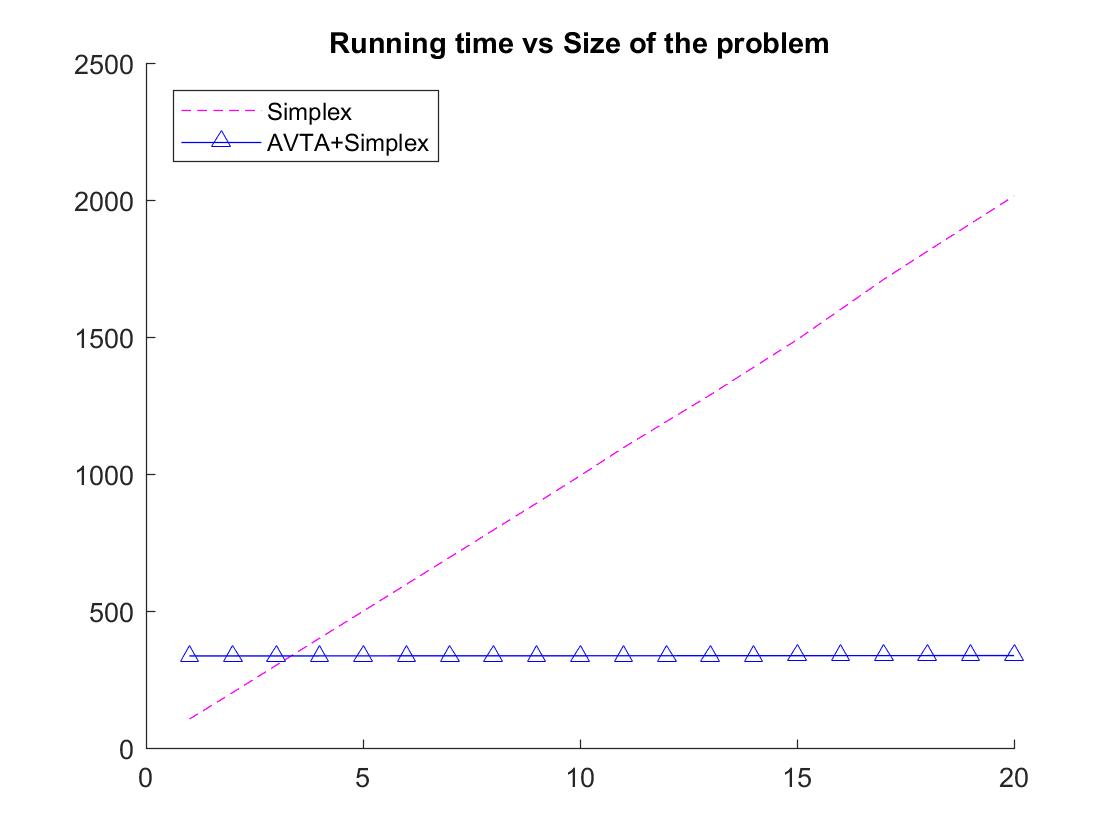
Non-negative linear system: The non-negative linear system problem is to find a feasible solution of :
| (109) | ||||
In another word, to test if where are columns of . In case when is over complete, any feasible can be represented using only the generators of the set . By scaling so that columns of are in a dimensional hyperlane , one can find the generators of by finding the vertices of the convex hull of the projected points. This could be done efficiently by AVTA. Suppose we have a linear system and series of query points , it is sufficient to run AVTA once for dimension reduction and solve the subproblem using simplex method. We compare the running time of Simplex Method with AVTA+Simplex Method. The generator is entrywise independent random matrix and the ’overcomplete’ part of the matrix are generated by where is entrywise independent random matrix. We set the number of generators , the dimension , and the number of ’redundant’ columns . We simply set half of the query points feasible and rest infeasible. The feasible points are generated as where is entrywise independent random vector and the infeasible points are generated in the same way as generators.
|
AVTA+Simplex | Simplex | # of query | AVTA+Simplex | Simplex | ||
| 1.00 | 241.24 | 152.09 | 11.00 | 241.94 | 1810.72 | ||
| 2.00 | 241.36 | 303.86 | 12.00 | 242.01 | 1967.93 | ||
| 3.00 | 241.41 | 477.89 | 13.00 | 242.07 | 2125.62 | ||
| 4.00 | 241.45 | 660.95 | 14.00 | 242.16 | 2289.91 | ||
| 5.00 | 241.54 | 853.91 | 15.00 | 242.23 | 2490.52 | ||
| 6.00 | 241.61 | 1016.77 | 16.00 | 242.29 | 2680.61 | ||
| 7.00 | 241.69 | 1177.30 | 17.00 | 242.32 | 2866.23 | ||
| 8.00 | 241.72 | 1336.38 | 18.00 | 242.41 | 3065.50 | ||
| 9.00 | 241.83 | 1495.70 | 19.00 | 242.44 | 3245.78 | ||
| 10.00 | 241.91 | 1652.84 | 20.00 | 242.47 | 3412.39 |
8.2 Computing all vertices
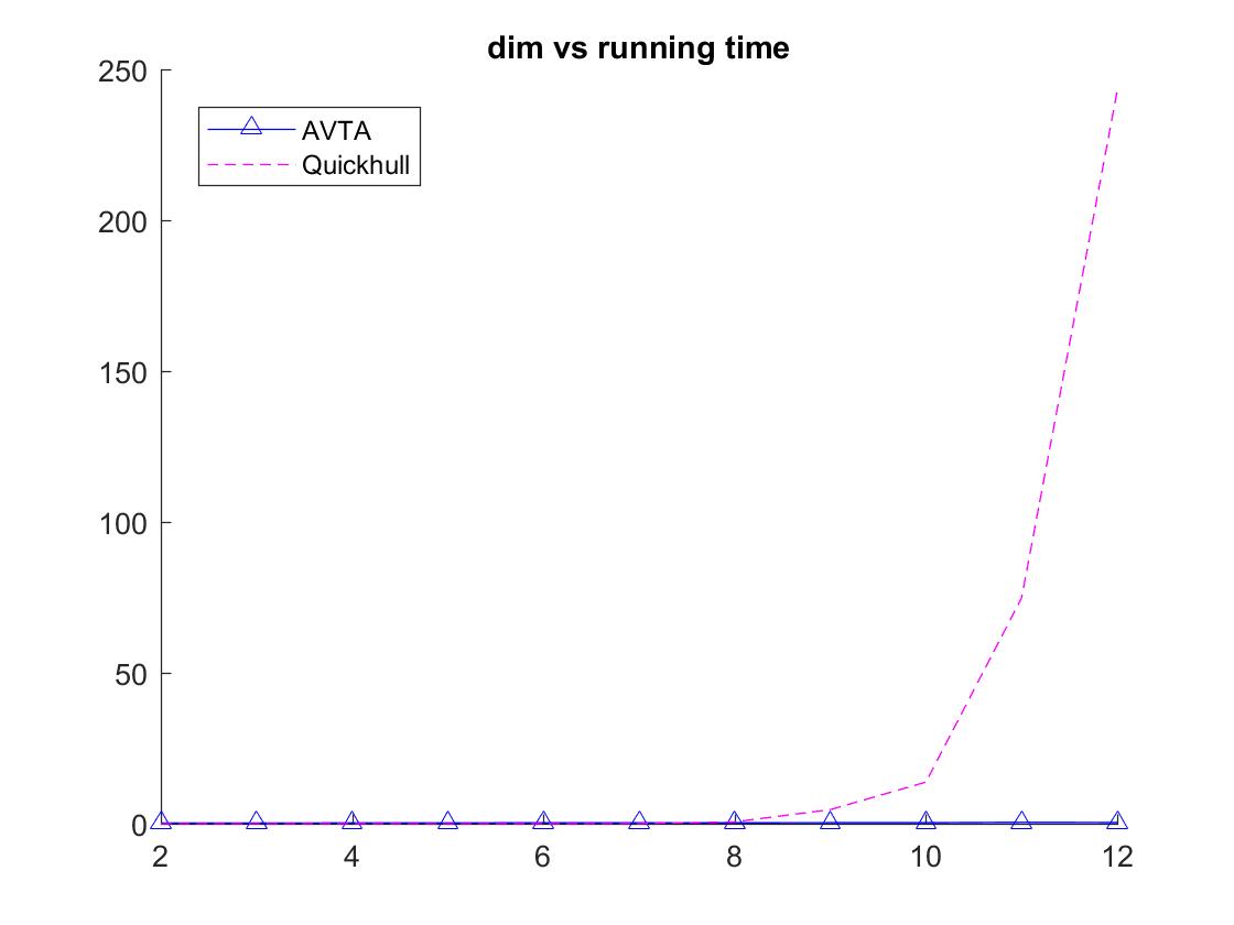
Compute vertices of convex hull: In this section, we compare the efficiency of AVTA with another popular algorithm for finding vertices Quickhull Barber et al. (1996). We generate vertices according to a Gaussian distribution . Having generated such points, interior points are generated as convex combination of the vertices, where the weights are generated scaled i.i.d uniform distribution.
Experiment and results: In the experiment, we set , and varying from . 333 The maximum of dimension is in the experiment because of the explosion of running time of the Quick hull algorithm. The computational results is shown in Table 4. In high dimension , when is robust for some , the AVTA algorithm successfully find all vertices of the convex hull efficiently while the Quick hull algorithm is stuck by its explosion of complexity in dimension .
| dim | Qhull | AVTA | dim | Qhull | AVTA |
|---|---|---|---|---|---|
| 2 | 0.13 | 14.82 | 7 | 2.92 | 41.51 |
| 3 | 0.02 | 16.62 | 8 | 16.48 | 39.63 |
| 4 | 0.04 | 24.49 | 9 | 82.09 | 44.21 |
| 5 | 0.12 | 32.76 | 10 | 391.36 | 45.79 |
| 6 | 0.59 | 37.66 | 11 | 1479.51 | 51.19 |
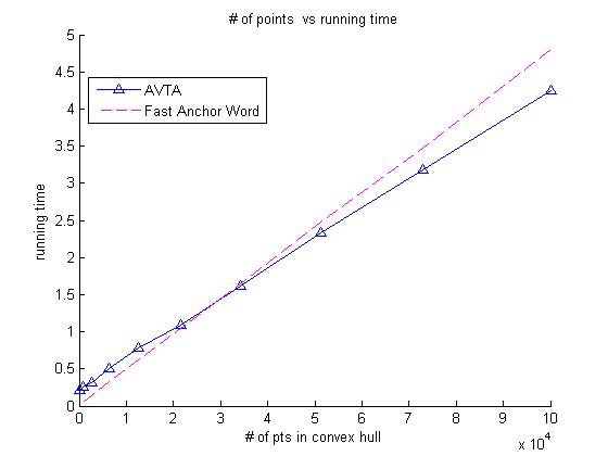
Compute vertices of simplex in high dimension: The Fast Anchor Word can be used to detect the vertices of a simplex. In this section, we compare the efficiency of AVTA with Fast Anchor Word when convex hull is a simplex with and . The number of points in the convex hull varies from .
Results of running time in simplex case: The running of efficiency comparison between AVTA and Fast Anchor Word in simplex case is presented in Figure 6(c). In regime , AVTA has less running time.
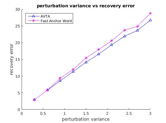
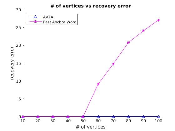
Compute vertices with perturbation: In this section, we compare the robustness of AVTA with multiple random projections presented in section 7 with Fast Anchor Word Arora et al. (2013). Instead of actual set of points as input, the algorithm is given a perturbed set , i.e. is corrupted by some noise. Having fixed ,, , we choose a Gaussian perturbation from where varies from to . In case of general convex hull, a failure of Fast Anchor Word on computing vertices of general convex hull is presented. The data is generated by setting , , and let varies from . We do an error analysis and evaluate the output of the algorithms by measuring the distance between true vertices and the convex hull of output vertices of the two algorithms. More precisely, given a true vertex and , the output of an algorithm, the error in recovering is defined to be We add up all the errors to get the total accumulated error.
Results on computing perturbed vertices:
The recovery error in robustness comparison is shown in Table 5. The AVTA with multiple random projection has a better recovery error in the simplex case.
It can also be observed from Figure 6(b) that in general case, as number of vertices exceeds the number of dimensions, Fast Anchor Word fails to recover more vertices and its error explodes.
| Var | AVTA+Multiple Rp | Fast Anhor | variance | AVTA+Multiple Rp | Fast Anhor |
| 0.3 | 2.96 | 2.96 | 1.8 | 16.60 | 17.98 |
| 0.6 | 5.79 | 5.79 | 2.1 | 19.40 | 20.58 |
| 0.9 | 8.61 | 9.36 | 2.4 | 21.93 | 23.77 |
| 1.2 | 11.34 | 12.00 | 2.7 | 23.69 | 24.90 |
| 1.5 | 14.16 | 15.44 | 3 | 26.72 | 28.78 |
8.3 Topic modeling
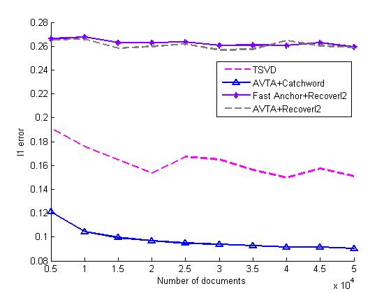
We compare our algorithms with the Fast Anchor + Recoverl2 algorithm of Arora et al. (2013) and the TSVD algorithm of Bansal et al. (2014) on two types of data sets: semi-synthetic data and real world data. We next describe our methodology and empirical results in detail.
Semi Synthetic Data: For Semi-Synthetic data set, we use similar methodology as in Arora et al. (2013). We first train the model on real data set using Gibbs sampling with iterations. We choose as the number of topics which follows Bansal et al. (2014). Given the parameters learned from dataset, we generate documents with set to be . The average document length is . Then the reconstruction error is measured by the distance of bipartite matched pairs between the true word-topic distribution and the word-topic distribution Arora et al. (2013). We then average the errors to compute the final mean error.
Real Data: We use the NIPS data set with 1500 documents , and a pruned vocabulary of 2K words, and the NYTimes Corpus with sub sampled documents, and a pruned vocabulary of 5k words. 444https://archive.ics.uci.edu/ml/datasets/bag+of+words. For the real world data set, as in prior works Arora et al. (2013); Bansal et al. (2014), we evaluate the coherence to measure topic quality Yao et al. (2009). Given a set of words associated with a learned topic, the coherence is computed as: , where and are the number of documents where appears and appear together respectively Arora et al. (2013), and is set to to avoid that never co-occur Stevens et al. (2012). The total coherence is the sum of the coherence of each topic. In the NIPS dataset, out of the documents were selected as the training set to learn the word-topic distributions. The rest of the documents were used as the testing set.
Implementation Details: We compare 4 algorithms, AVTA+CatchWord, TSVD, the Fast Anchor + Recoverl2 and the AVTA+Recoverl2. We implement our own version of Fast Anchor + Recoverl2 as described in Arora et al. (2013). TSVD is implemented using the code provided by the authors in Bansal et al. (2014). AVTA+Recoverl2 corresponds to using AVTA to detect anchor words from the word-word covariance matrix and then using the Recoverl2 procedure from Arora et al. (2013) to get the topic-word matrix. AVTA + CatchWord corresponds to finding the low dimensional embedding of each document in terms of the coefficient vector of its representation in the convex hull of the vertices. The next step is to cluster these points. In practice, one could use the Lloyd’s algorithm for this step which could be sensitive to initialization. To remedy this, we use similar heuristic as Bansal et al. (2014) of the initialization step. We repeat AVTA for times and pick the set of vertices with highest quality where the quality is measured by sum of distances of each vertex to convex hull of other vertices. We set the number of output vertices which is the same as the number of topics. i.e. each vertex corresponds to a topic. We found that initializing by simply assigning clusters using neighborhoods of highest degree vertices works effectively. As a final step, we use the post processing step from Bansal et al. (2014) to recover the topic-word matrix from the clustering.
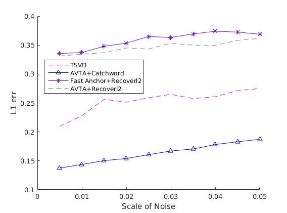
Robustness: We also generate perturbed version of the semi synthetic data. We generate a random matrix with i.i.d. entries uniformly distributed with different scales varying from . We test all the algorithms with the document-word matrix added with the noise matrix.
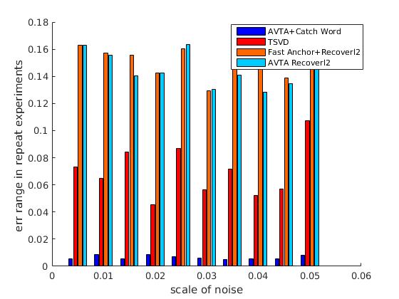
Results on Semi Synthetic Data: Figures 6(d) and 6(e) show the reconstruction of all the four algorithms under both clean and noisy versions of the semi synthetic data set. For topic , let be the ground truth topic vector and be the topic vector recovered by the algorithm. Then the error is defined as . The plots show that AVTA+CatchWord is consistently better than both TSVD and Fast Anchor + Recoverl2 and produces significantly more accurate topic vectors. In order to further test the robustness of our approach, we plot in Figure 6(f) the range of the error obtained across multiple runs of the algorithms on the same data set. The range is defined to be the difference between the maximum and the minimum error recovered by the algorithm across different runs. We see that AVTA+CatchWord produces solutions that are much more stable to the effect of the noise as compared to other algorithms. Table 6 shows the running time of the experiments of 4 algorithms. As can be seen, when using AVTA to learn topic models via the anchor words approach, our algorithm has comparable run time to Fast Anchor + Recoverl2. In CatchWord based learning, computing vertices is expensive compared to K-SVD step of TSVD thus AVTA has longer running time.
|
5,000 | 15,000 | 30,000 | 50,000 | ||
|---|---|---|---|---|---|---|
| Fast anchor+Recoverl2 | 5.49 | 6.00 | 10.30 | 13.60 | ||
| AVTA+Recoverl2 | 7.82 | 7.68 | 12.84 | 16.40 | ||
| TSVD | 17.02 | 43.27 | 81.24 | 112.80 | ||
| AVTA+Catch Word | 29.89 | 120.04 | 372.17 | 864.30 |
Results on Real Data: Table 7 shows the topic coherence obtained by the algorithms. One can see that in both the approaches, either via anchor words or the clustering approach, AVTA based algorithms perform comparably to state of the art methods 555The topic coherence results for TSVD do not match the ones presented in Bansal et al. (2014) since in their experiments, the authors look at top 10 most frequent words in each topic. In our experiments we compute coherence for the top 5 most frequent words in each topic.. The running time is presented in Table 8. The AVTA+CathchWord has less running time in the real data experiments. Per our observation, the convex hull of word-document vectors in real data set has more vertices than , the number of topics. The AVTA catches vertices efficiently due to its small number of iterations on line search for . In semi-synthetic data set, the number of ’robust’ vertices is approximately the same as number of topics thus AVTA needs to find almost all vertices. To catch enough vertices, AVTA needs several iterations decreasing which is computationally expensive.
8.4 Non-negative matrix factorization
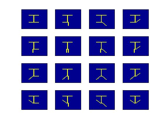
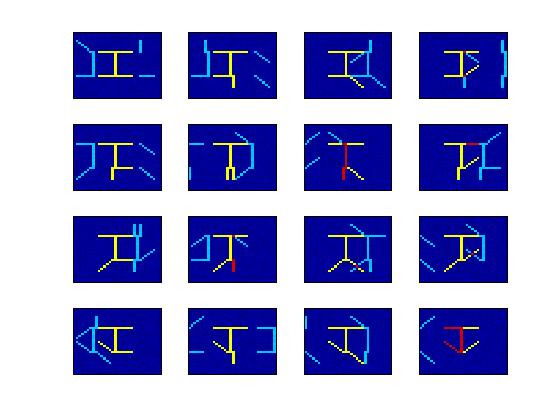
AVTA for NMF: For our experiments on NMF we use the Swimmer data set Donoho and Stodden (2003) that consists of swimmer figures with each a binary pixel images. One can interpret each image as a document and pixels as a word in the document Ding et al. (2013). All swimmers consist of limbs with each limb having different possible poses. One can then consider the different poses of limbs as the true underlying topics Donoho and Stodden (2003). We compare the algorithm proposed in Arora et al. (2012a) with AVTA+Recoverl2 on the swimmer data set. We construct a noisy version by adding spurious poses to original swimmer data set. Let be a function that outputs a randomly chosen block of an image. We generate a ’spurious pose’ of size by where is a randomly chosen swimmer image. Then we take another randomly chosen image and compute the corrupted image as where we simply set . An illustration of the noise data set is shown in Figure 7(b). Since the true underlying topics are known, we will plot the output of the algorithms and compare it with the underlying truth.
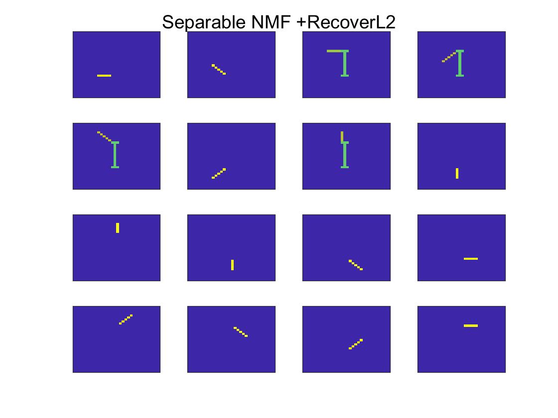
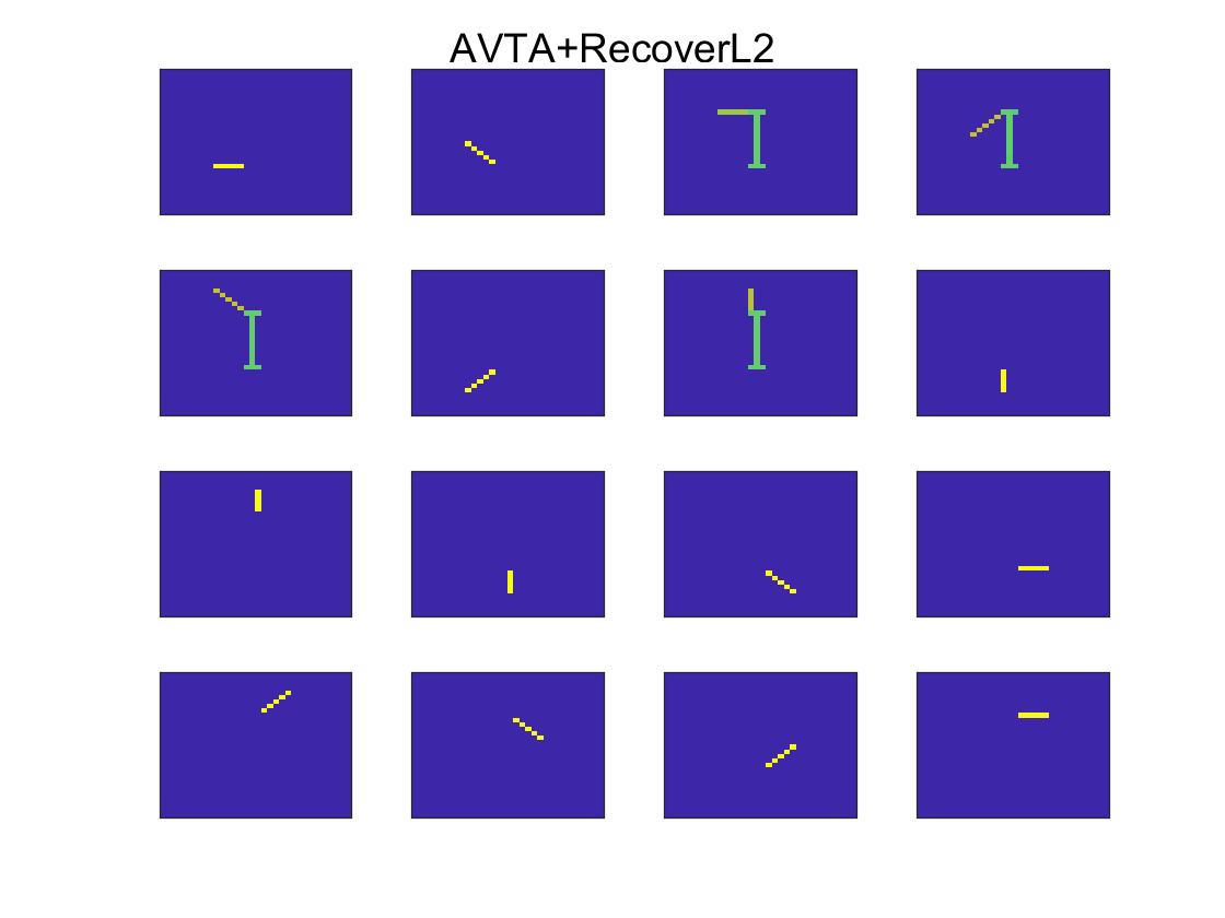
Results on NMF: We compare the performance of AVTA on these data sets with the performance of the Separable NMF algorithm proposed in Arora et al. (2012a). Figures 7(c) and 7(d) show the output of the Separable NMF algorithm and that of our algorithm respectively on the noisy data set. Our approach produces competitive results as compared to the Separable NMF algorithm.
| Fast Anchor+RecoverL2 | AVTA+RecoverL2 | TSVD | AVTA+Catch Word | |
|---|---|---|---|---|
| NIPS | -15.8 | -16.04 | -16.86 | -18.65 |
| NYTimes | -32.15 | -32.13 | -29.39 | -30.13 |
| Fast Anchor+RecoverL2 | AVTA+RecoverL2 | TSVD | AVTA+Catch Word | |
|---|---|---|---|---|
| NIPS | 3.22 | 4.41 | 56.58 | 22.78 |
| NYTimes | 26.05 | 27.79 | 237.6 | 101.07 |
9 Conclusion
In this work we have presented a fast and robust algorithm for computing the vertices of the convex hull of a set of points. Our algorithm efficiently computes the vertices of convex hulls in high dimensions and even in the special case of the simplex is competitive with the state of the art approaches in terms of running time Arora et al. (2013). Furthermore, our algorithm leads to an improved algorithm for topic modeling that is more robust and produces better approximations to the topic-word matrix. It will be interesting to provide theoretical claims supporting this observation in the context of specific applications. Furthermore, we believe that our algorithm will have more applications in machine learning problems beyond the ones investigated here as well as applications in computational geometry and in linear programming.
References
- Anandkumar et al. (2012) Anima Anandkumar, Dean P Foster, Daniel J Hsu, Sham M Kakade, and Yi-Kai Liu. A spectral algorithm for latent dirichlet allocation. In Advances in Neural Information Processing Systems, pages 917–925, 2012.
- Arora et al. (2012a) Sanjeev Arora, Rong Ge, Ravindran Kannan, and Ankur Moitra. Computing a nonnegative matrix factorization–provably. In Proceedings of the forty-fourth annual ACM symposium on Theory of computing, pages 145–162. ACM, 2012a.
- Arora et al. (2012b) Sanjeev Arora, Rong Ge, and Ankur Moitra. Learning topic models–going beyond svd. In Foundations of Computer Science (FOCS), 2012 IEEE 53rd Annual Symposium on, pages 1–10. IEEE, 2012b.
- Arora et al. (2013) Sanjeev Arora, Rong Ge, Yonatan Halpern, David Mimno, Ankur Moitra, David Sontag, Yichen Wu, and Michael Zhu. A practical algorithm for topic modeling with provable guarantees. In International Conference on Machine Learning, pages 280–288, 2013.
- Arora et al. (2014) Sanjeev Arora, Rong Ge, and Ankur Moitra. New algorithms for learning incoherent and overcomplete dictionaries. In COLT, pages 779–806, 2014.
- Awasthi and Risteski (2015) Pranjal Awasthi and Andrej Risteski. On some provably correct cases of variational inference for topic models. In Advances in Neural Information Processing Systems, pages 2098–2106, 2015.
- Bansal et al. (2014) Trapit Bansal, Chiranjib Bhattacharyya, and Ravindran Kannan. A provable svd-based algorithm for learning topics in dominant admixture corpus. In Advances in Neural Information Processing Systems, pages 1997–2005, 2014.
- Barber et al. (1996) C Bradford Barber, David P Dobkin, and Hannu Huhdanpaa. The quickhull algorithm for convex hulls. ACM Transactions on Mathematical Software (TOMS), 22(4):469–483, 1996.
- Blei (2012) David M Blei. Probabilistic topic models. Communications of the ACM, 55(4):77–84, 2012.
- Blei et al. (2003) David M Blei, Andrew Y Ng, and Michael I Jordan. Latent dirichlet allocation. Journal of machine Learning research, 3(Jan):993–1022, 2003.
- Blum et al. (2016) Avrim Blum, Sariel Har-Peled, and Benjamin Raichel. Sparse approximation via generating point sets. In Proceedings of the twenty-seventh annual ACM-SIAM symposium on Discrete algorithms, pages 548–557. Society for Industrial and Applied Mathematics, 2016.
- Burges (1998) Christopher JC Burges. A tutorial on support vector machines for pattern recognition. Data mining and knowledge discovery, 2(2):121–167, 1998.
- Chan (1996a) Timothy M Chan. Optimal output-sensitive convex hull algorithms in two and three dimensions. Discrete & Computational Geometry, 16(4):361–368, 1996a.
- Chan (1996b) Timothy M Chan. Output-sensitive results on convex hulls, extreme points, and related problems. Discrete & Computational Geometry, 16(4):369–387, 1996b.
- Chazelle (1993) Bernard Chazelle. An optimal convex hull algorithm in any fixed dimension. Discrete & Computational Geometry, 10(1):377–409, 1993.
- Chvatal (1983) Vasek Chvatal. Linear programming. Macmillan, 1983.
- Clarkson (1994) Kenneth L Clarkson. More output-sensitive geometric algorithms. In Foundations of Computer Science, 1994 Proceedings., 35th Annual Symposium on, pages 695–702. IEEE, 1994.
- Clarkson (2010) Kenneth L Clarkson. Coresets, sparse greedy approximation, and the frank-wolfe algorithm. ACM Transactions on Algorithms (TALG), 6(4):63, 2010.
- Ding et al. (2013) Weicong Ding, Mohammad Hossein Rohban, Prakash Ishwar, and Venkatesh Saligrama. Topic discovery through data dependent and random projections. In ICML (3), pages 1202–1210, 2013.
- Donoho and Stodden (2003) David Donoho and Victoria Stodden. When does non-negative matrix factorization give a correct decomposition into parts? In Advances in Neural Information Processing Systems, 2003.
- Frank and Wolfe (1956) Marguerite Frank and Philip Wolfe. An algorithm for quadratic programming. Naval Research Logistics (NRL), 3(1-2):95–110, 1956.
- Gärtner and Jaggi (2009) Bernd Gärtner and Martin Jaggi. Coresets for polytope distance. In Proceedings of the twenty-fifth annual symposium on Computational geometry, pages 33–42. ACM, 2009.
- Gilbert (1966) Elmer G Gilbert. An iterative procedure for computing the minimum of a quadratic form on a convex set. SIAM Journal on Control, 4(1):61–80, 1966.
- Har-Peled et al. (2007) Sariel Har-Peled, Dan Roth, and Dav Zimak. Maximum margin coresets for active and noise tolerant learning. In IJCAI, pages 836–841, 2007.
- Jaggi (2013) Martin Jaggi. Revisiting frank-wolfe: Projection-free sparse convex optimization. 2013.
- Jarvis (1973) Ray A Jarvis. On the identification of the convex hull of a finite set of points in the plane. Information Processing Letters, 2(1):18–21, 1973.
- Jin and Kalantari (2006) Yi Jin and Bahman Kalantari. A procedure of chvátal for testing feasibility in linear programming and matrix scaling. Linear algebra and its applications, 416(2-3):795–798, 2006.
- Johnson and Lindenstrauss (1984) William B Johnson and Joram Lindenstrauss. Extensions of lipschitz mappings into a hilbert space. Contemporary mathematics, 26(189-206):1, 1984.
- Kalantari (2015) Bahman Kalantari. A characterization theorem and an algorithm for a convex hull problem. Annals of Operations Research, 226(1):301–349, 2015.
- Karmarkar (1984) Narendra Karmarkar. A new polynomial-time algorithm for linear programming. In Proceedings of the sixteenth annual ACM symposium on Theory of computing, pages 302–311. ACM, 1984.
- Khachiyan (1980) Leonid G Khachiyan. Polynomial algorithms in linear programming. USSR Computational Mathematics and Mathematical Physics, 20(1):53–72, 1980.
- Lee and Seung (2001) Daniel D Lee and H Sebastian Seung. Algorithms for non-negative matrix factorization. In Advances in neural information processing systems, pages 556–562, 2001.
- Matoušek and Schwarzkopf (1992) Jiří Matoušek and Otfried Schwarzkopf. Linear optimization queries. In Proceedings of the eighth annual symposium on Computational geometry, pages 16–25. ACM, 1992.
- Olshausen and Field (1996) Bruno A Olshausen and David J Field. Emergence of simple-cell receptive field properties by learning a sparse code for natural images. Nature, 381(6583):607, 1996.
- Papadimitriou et al. (1998) Christos H Papadimitriou, Hisao Tamaki, Prabhakar Raghavan, and Santosh Vempala. Latent semantic indexing: A probabilistic analysis. In Proceedings of the seventeenth ACM SIGACT-SIGMOD-SIGART symposium on Principles of database systems, pages 159–168. ACM, 1998.
- Spielman et al. (2012) Daniel A Spielman, Huan Wang, and John Wright. Exact recovery of sparsely-used dictionaries. In COLT, pages 37–1, 2012.
- Stevens et al. (2012) Keith Stevens, Philip Kegelmeyer, David Andrzejewski, and David Buttler. Exploring topic coherence over many models and many topics. In Proceedings of the 2012 Joint Conference on Empirical Methods in Natural Language Processing and Computational Natural Language Learning, pages 952–961. Association for Computational Linguistics, 2012.
- Toth et al. (2004) Csaba D Toth, Joseph O’Rourke, and Jacob E Goodman. Handbook of discrete and computational geometry. CRC press, 2004.
- Toussaint (1983) Godfried T Toussaint. Solving geometric problems with the rotating calipers. In Proc. IEEE Melecon, volume 83, page A10, 1983.
- Vu et al. (2017) Ky Vu, Pierre-Louis Poirion, and Leo Liberti. Random projections for linear programming. arXiv preprint arXiv:1706.02768, 2017.
- Yao et al. (2009) Limin Yao, David Mimno, and Andrew McCallum. Efficient methods for topic model inference on streaming document collections. In Proceedings of the 15th ACM SIGKDD international conference on Knowledge discovery and data mining, pages 937–946. ACM, 2009.
- Zhang (2003) Tong Zhang. Sequential greedy approximation for certain convex optimization problems. IEEE Transactions on Information Theory, 49(3):682–691, 2003.