Image denoising with generalized Gaussian mixture model patch priors

Abstract

Patch priors have become an important component of image restoration. A powerful approach in this category of restoration algorithms is the popular Expected Patch Log-Likelihood (EPLL) algorithm. EPLL uses a Gaussian mixture model (GMM) prior learned on clean image patches as a way to regularize degraded patches. In this paper, we show that a generalized Gaussian mixture model (GGMM) captures the underlying distribution of patches better than a GMM. Even though GGMM is a powerful prior to combine with EPLL, the non-Gaussianity of its components presents major challenges to be applied to a computationally intensive process of image restoration. Specifically, each patch has to undergo a patch classification step and a shrinkage step. These two steps can be efficiently solved with a GMM prior but are computationally impractical when using a GGMM prior. In this paper, we provide approximations and computational recipes for fast evaluation of these two steps, so that EPLL can embed a GGMM prior on an image with more than tens of thousands of patches. Our main contribution is to analyze the accuracy of our approximations based on thorough theoretical analysis. Our evaluations indicate that the GGMM prior is consistently a better fit for modeling image patch distribution and performs better on average in image denoising task.

68U10, 62H35, 94A08

1 Introduction

Image restoration is the process of recovering the underlying clean image from its degraded or corrupted observation(s). The images captured by common imaging systems often contain corruptions such as noise, optical or motion blur due to sensor limitations and/or environmental conditions. For this reason, image restoration algorithms have widespread applications in medical imaging, satellite imaging, surveillance, and general consumer imaging applications. Priors on natural images play an important role in image restoration algorithms. Image priors are used to denoise or regularize ill-posed restoration problems such as deblurring and super-resolution, to name just a few. Early attempts in designing image priors relied on modeling local pixel gradients with Gibbs distributions [25], Laplacian distributions (total variation) [54, 65], hyper-Laplacian distribution [31], generalized Gaussian distribution [7], or Gaussian mixture models [21]. Concurrently, priors have also been designed by modeling coefficients of an image in a transformed domain using generalized Gaussian [35, 40, 9, 15] or scaled mixture of Gaussian [49] priors for wavelet or curvelet coefficients [6]. Alternatively, modeling the distribution of patches of an image (i.e., small windows usually of size $8\times 8$) has proven to be a powerful solution. In particular, popular patch techniques rely on non-local self-similarity [8], fields of experts [52], learned patch dictionaries [2, 19, 53], sparse or low-rank properties of stacks of similar patches [12, 13, 34, 29], patch re-occurrence priors [37], or more recently mixture models patch priors [67, 66, 61, 60, 26, 56, 44].

Of these approaches, a successful approach introduced by Zoran and Weiss [67] is to model patches of clean natural images using Gaussian Mixture Model (GMM) priors. The agility of this model lies in the fact that a prior learned on clean image patches can be effectively employed to restore a wide range of inverse problems. It is also easily extendable to include other constraints such as sparsity or multi-resolution patches [58, 45]. The use of GMMs for patch priors make these methods computationally tractable and flexible. Although GMM patch prior is effective and popular, in this article, we argue that a generalized Gaussian mixture model (GGMM) is a better fit for image patch prior modeling. Compared to a Gaussian model, a generalized Gaussian distribution (GGD) has an extra degree of freedom controlling the shape of the distribution and it encompasses Gaussian and Laplacian models.

Beyond image restoration tasks, GGDs have been used in several different fields of image and signal processing, including watermark detection [11], texture retrieval [15], voice activity detection [23] and MP3 audio encoding [16], to cite just a few. In these tasks, GGDs are used to characterize or model the prior distribution of clean signals, for instance, from their DCT coefficients or frequency subbands for natural images [63, 59, 41, 3] or videos [55], gradients for X-ray images [7], wavelet coefficients for natural [35, 40, 11], textured [15], or ultrasound images [1], tangential wavelet coefficients for three-dimensional mesh data [33], short time windows for speech signals [30] or frequency subbands for speech [23] or audio signals [16].

In this paper, we go one step further and use multi-variate GGD with one scale and one shape parameter per dimension. The superior patch prior modeling capability of such a GGMM over a GMM is illustrated in Figure 1. The figure shows histograms of six orthogonal 1-D projections of subset of clean patches onto the eigenvectors of the covariance matrix of a single component of the GMM. To illustrate the difference in the shapes ($\nu$) and scales ($\lambda$) of the distributions of each dimension, we have chosen a few projections corresponding to both the most and the least significant eigenvalues. It can be seen that GGD is a better fit on the obtained histograms than a Gaussian model. Additionally, different dimensions of the patch follow a different GGD (i.e., has a different shape and scale parameter). Hence, it does not suffice to model all the feature dimensions of a given cluster of patches as Laplacian or Gaussian. Therefore, we propose to model patch priors as GGMM distributed with a separate shape and scale parameters for each feature dimension of a GGD component. This differs from the recent related approach in [44] that considered GGMM where each component has a fixed shape parameter for all directions.

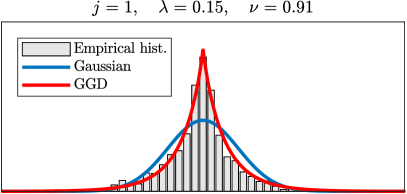
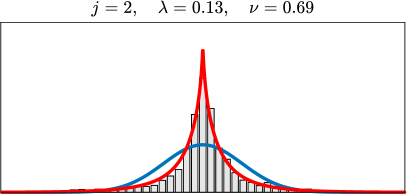
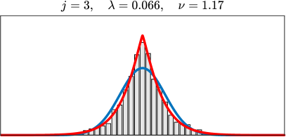
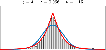
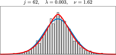
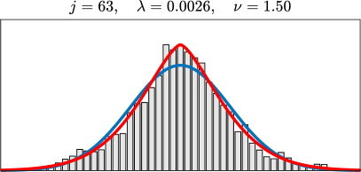
Figure 1: Histograms of the projection of $200,000$ clean patches on 6 eigenvectors $j=1,2,3,4,62$ and $63$ of the covariance matrix of one component $k$ of the mixture (with weight $w_{k}=1.3$%). The contribution of each clean patch in the histograms is given by its membership values onto this component $k$ (as obtained during the E-Step of EM). For each histogram, a generalized Gaussian distribution was adjusted by estimating the parameters $\lambda$ and $\nu$ by moment estimation (as obtained during the M-Step of our modified EM exposed in Section 3.1). For comparisons, we have also provided illustrations of the best fit obtained with a Gaussian distribution.

Contributions

The goal of this paper is to measure the improvements obtained in image denoising tasks by incorporating a GGMM in EPLL algorithm. Unlike [44], that incorporates a GGMM prior in a posterior mean estimator based on importance sampling, we directly extend the maximum a posteriori formulation of Zoran and Weiss [67] for the case of GGMM priors. While such a GGMM prior has the ability to capture the underlying distribution of clean patches more closely, we will show that it introduces two major computational challenges in this case. The first one can be thought of as a classification task in which a noisy patch is assigned to one of the components of the mixture. The second one corresponds to an estimation task where a noisy patch is denoised given that it belongs to one of the components of the mixture. Due to the interaction of the noise distribution with the GGD prior, we first show that these two tasks lead to a group of one-dimensional integration and optimization problems, respectively. Specifically, for $x\in\mathbb{R}$, these problems are of the following forms

(1) $$\int_{\mathbb{R}}\exp\left(-\frac{(t-x)^{2}}{2\sigma^{2}}-\frac{|t|^{\nu}}{\lambda_{\nu}^{\nu}}\right)\;\mathrm{d}t\quad\quad\text{and}\quad\quad\underset{t\in\mathbb{R}}{\operatorname{argmin}}\;\frac{(t-x)^{2}}{2\sigma^{2}}+\frac{|t|^{\nu}}{\lambda_{\nu}^{\nu}}~{},$$

for some $\nu>0$, $\sigma>0$ and $\lambda_{\nu}>0$. In general, they do not admit closed-form solutions but some particular solutions or approximations have been derived for the estimation/optimization problem [40, 10]. By contrast, up to our knowledge, little is known for approximating the classification/integration one (only crude approximations were proposed in [57]).

Our contributions are both theoretical- and application-oriented. The major contribution of this paper, which is and theoretical in nature, is to develop an accurate approximation for the classification/integration problem. In particular, we show that our approximation error vanishes for $x\to 0$ and $x\to\pm\infty$ when $\nu=1$, see 1 and 2. We next generalize this result for $\frac{2}{3}<\nu<2$ in 3 and 4. On top of that, we prove that the two problems enjoy some important desired properties in 2 and 3. These theoretical results allow the two quantities to be approximated by functions that can be quickly evaluated in order to be incorporated in fast algorithms. Our last contribution is experimental and concerns the performance evaluation of the proposed model in image denoising scenario. For reproducibility, we have released our implementation at https://bitbucket.org/cdeledalle/ggmm-epll.

Potential impacts beyond image denoising

It is important to note that the two main contributions presented in this work, namely approximations for classification and estimation problems, are general techniques that are relevant to a wider area of research problems than image restoration. In particular, our contributions apply to any problems where (i) the underlying clean data are modeled by a GGD or a GGMM, whereas (ii) the observed samples are corrupted by Gaussian noise. They are especially relevant in machine learning scenarios where a GGMM is trained on clean data but data provided during testing time is noisy. That is, our approximations can be used to extend the applicability of the aforementioned clean GGD/GGM based approaches to the less than ideal testing scenario where the data is corrupted by noise. For instance, using the techniques introduced in this paper, one could directly use the GGD based voice activity model of [23] into the likelihood ratio test based detector of [22] (which relies on solutions of the integration problem but was limited to Laplacian distributions). In fact, we suspect that many studies in signal processing may have limited themselves to Gaussian or Laplacian signal priors because of the complicated integration problem arising from the intricate interaction of GGDs with Gaussian noise. In this paper, we demonstrate that this difficulty can be efficiently overcome with our approximations. This leads us to believe that the impact of the approaches presented in this paper will not only be useful for image restoration but also aid a wider field of general signal processing applications.

Organization

After explaining the considered patch prior based restoration framework in Section 2, we derive our GGMM based restoration scheme in Section 3. The approximations of the classification and estimation problems are studied in Section 4 and Section 5, respectively. Finally, we present numerical experiments and results in Section 6.

2 Background

In this section we provide a detailed overview of the use of patch-based priors in Expected Patch Log-Likelihood (EPLL) framework and its usage under GMM priors.

2.1 Image restoration with patch based priors

We consider the problem of estimating an image ${\boldsymbol{u}}\in\mathbb{R}^{N}$ ($N$ is the number of pixels) from noisy linear observations ${\boldsymbol{v}}=\mathcal{A}{\boldsymbol{u}}+{\boldsymbol{w}}$, where $\mathcal{A}:\mathbb{R}^{N}\to\mathbb{R}^{M}$ is a linear operator and ${\boldsymbol{w}}\in\mathbb{R}^{M}$ is a noise component assumed to be white and Gaussian with variance $\sigma^{2}$. In this paper, we will focus on standard denoising problems where $\mathcal{A}$ is the identity matrix, but in more general settings, it can account for loss of information such as blurring. Typical examples for operator $\mathcal{A}$ are: a low pass filter (for deconvolution), a masking operator (for inpainting), or a projection on a random subspace (for compressive sensing). To reduce noise and stabilize the inversion of $\mathcal{A}$, some prior information is used for the estimation of ${\boldsymbol{u}}$. Recent techniques [19, 67, 58] include this prior information as a model for the distribution of patches found in natural clean images. We consider the EPLL framework [67] that restores an image by maximum a posteriori estimation over all patches, corresponding to the following minimization problem:

(2) $$\underset{{\boldsymbol{u}}\in\mathbb{R}^{n}}{\operatorname{argmin}}\;\frac{P}{2\sigma^{2}}|\!|\mathcal{A}{\boldsymbol{u}}-{\boldsymbol{v}}|\!|^{2}-\sum_{i=1}^{N}\log p\left(\mathcal{P}_{i}{\boldsymbol{u}}\right)$$

where $\mathcal{P}_{i}:\mathbb{R}^{N}\to\mathbb{R}^{P}$ is the linear operator extracting a patch with $P$ pixels centered at the pixel with location $i$ (typically, $P=8\!\times\!8$), and $p(.)$ is the a priori probability density function (i.e., the statistical model of noiseless patches in natural images). Since $i$ scans all of the $N$ pixels of the image, all patches contribute to the loss and many patches overlap. Allowing for overlapping is important because otherwise there would appear blocking artifacts. While the first term in eq. (2) ensures that $\mathcal{A}{\boldsymbol{u}}$ is close to the observations ${\boldsymbol{v}}$ (this term is the negative log-likelihood under the white Gaussian noise assumption), the second term regularizes the solution ${\boldsymbol{u}}$ by favoring an image such that all of its patches fit the prior model of patches in natural images.

Optimization with half-quadratic splitting

Problem (2) is a large optimization problem where $\mathcal{A}$ couples all unknown pixel values of ${\boldsymbol{u}}$ and the patch prior is often chosen non-convex. Our method follow the choice made by EPLL of using a classical technique, known as half-quadratic splitting [24, 31], that introduces $N$ auxiliary unknown vectors ${\boldsymbol{z}}_{i}\in\mathbb{R}^{P}$, and alternatively consider the penalized optimization problem, for $\beta>0$, as

(3) $$\underset{\begin{subarray}{c}{\boldsymbol{u}}\in\mathbb{R}^{n}\\ {\boldsymbol{z}}_{1},\ldots,{\boldsymbol{z}}_{N}\in\mathbb{R}^{P}\end{subarray}}{\operatorname{argmin}}\;\frac{P}{2\sigma^{2}}|\!|\mathcal{A}{\boldsymbol{u}}-{\boldsymbol{v}}|\!|^{2}+\frac{\beta}{2}\sum_{i\in\mathcal{I}}|\!|\mathcal{P}_{i}{\boldsymbol{u}}-{\boldsymbol{z}}_{i}|\!|^{2}-\sum_{i\in\mathcal{I}}\log p\left({\boldsymbol{z}}_{i}\right).$$

When $\beta\to\infty$, the problem (3) is equivalent to the original problem (2). In practice, an increasing sequence of $\beta$ is considered, and the optimization is performed by alternating between the minimization for ${\boldsymbol{u}}$ and ${\boldsymbol{z}}_{i}$. Though little is known about the convergence of this algorithm, few iterations produce remarkable results, in practice. We follow the EPLL settings prescribed in [67] by performing 5 iterations of this algorithm with parameter $\beta$ set to $\frac{1}{\sigma^{2}}\{1,4,8,16,32\}$ for each iteration, respectively. The algorithm is initialized using $\hat{\boldsymbol{u}}={\boldsymbol{v}}$ for the first estimate.

Minimization with respect to ${\boldsymbol{u}}$

Considering all ${\boldsymbol{z}}_{i}$ to be fixed, optimizing (3) for ${\boldsymbol{u}}$ corresponds to solving a linear inverse problem with a Tikhonov regularization. It has an explicit solution known as the linear minimum mean square estimator (or often referred to as Wiener filtering) which is obtained as:

$$\hat{\boldsymbol{u}} =\underset{{\boldsymbol{u}}\in\mathbb{R}^{n}}{\operatorname{argmin}}\;\frac{P}{2\sigma^{2}}|\!|\mathcal{A}{\boldsymbol{u}}-{\boldsymbol{v}}|\!|^{2}+\frac{\beta}{2}\sum_{i\in\mathcal{I}}|\!|\mathcal{P}_{i}{\boldsymbol{u}}-\hat{\boldsymbol{z}}_{i}|\!|^{2}$$

(4) $$=\left(\mathcal{A}^{t}\mathcal{A}+\frac{\beta\sigma^{2}}{P}\sum_{i\in\mathcal{I}}\mathcal{P}_{i}^{t}\mathcal{P}_{i}\right)^{-1}\left(\mathcal{A}^{t}{\boldsymbol{v}}+\frac{\beta\sigma^{2}}{P}\sum_{i\in\mathcal{I}}\mathcal{P}_{i}^{t}\hat{\boldsymbol{z}}_{i}\right),$$

where $\mathcal{P}_{i}^{t}\mathcal{P}_{i}$ is a diagonal matrix whose $i$-th diagonal element corresponds to the number of patches overlapping the pixel of index $i$.

Minimization with respect to ${\boldsymbol{z}}_{i}$

Considering ${\boldsymbol{u}}$ to be fixed, optimizing (3) for ${\boldsymbol{z}}_{i}$ leads to:

(5) $$\hat{\boldsymbol{z}}_{i} \leftarrow\underset{{\boldsymbol{z}}_{i}\in\mathbb{R}^{P}}{\operatorname{argmin}}\;\frac{\beta}{2}|\!|\tilde{\boldsymbol{z}}_{i}-{\boldsymbol{z}}_{i}|\!|^{2}-\log p({\boldsymbol{z}}_{i})\quad\text{where}\quad\tilde{\boldsymbol{z}}_{i}=\mathcal{P}_{i}\hat{\boldsymbol{u}}~{},$$

which corresponds to the maximum a posterior (MAP) denoising problem under the patch prior $p$ of a patch $\tilde{\boldsymbol{z}}_{i}$ contaminated by Gaussian noise with variance $1/\beta$. The solution of this optimization problem strongly depends on the properties of the chosen patch prior.

Our algorithm will follow the exact same procedure as EPLL by alternating between eq. (2.1) and (5). In our proposed method, we will be using a generalized Gaussian mixture model (GGMM) to represent patch prior. The general scheme we will adopt to solve eq. (5) under GGMM prior is inspired from the one proposed by Zoran & Weiss [67] in the simpler case of Gaussian mixture model (GMM) prior. For this reason, we will now introduce this simpler case of GMM prior before exposing the technical challenges arising from the use of GGMM prior in Section 3.

2.2 Patch denoising with GMM priors

The authors of [67, 66] suggested using a zero-mean Gaussian mixture model (GMM) prior, that, for any patch ${\boldsymbol{z}}\in\mathbb{R}^{P}$, is given by

(6) $$p\left({\boldsymbol{z}}\right)=\sum_{k=1}^{K}w_{k}\mathcal{N}_{P}({\boldsymbol{z}};0_{P},{\boldsymbol{\Sigma}}_{k})$$

where $K$ is the number of components, $w_{k}>0$ are weights such that $\sum_{k}w_{k}\!=\!1$, and $\mathcal{N}_{P}(0_{P},{\boldsymbol{\Sigma}}_{k})$ denotes the multi-variate Gaussian distribution with zero-mean and covariance ${\boldsymbol{\Sigma}}_{k}\in\mathbb{R}^{P\times P}$. A $K$-component GMM prior models image patches as being spread over $K$ clusters that have ellipsoid shapes where each coefficient (of each component) follows a Gaussian distribution, i.e., bell-shaped with small tails. In [67], the parameters $w_{k}$ and ${\boldsymbol{\Sigma}}_{k}$ of the GMM are learned using the Expectation Maximization algorithm [14] on a dataset of 2 million clean patches of size $8\times 8$ pixels that are randomly extracted from the training images of the Berkeley Segmentation Database (BSDS) [36]. The GMM learned in [67] has $K=200$ zero-mean Gaussian mixture components.

Due to the multi-modality of the GMM prior, introducing this prior in eq. (5) makes the optimization problem highly non-convex:

(7) $$\hat{\boldsymbol{z}} \leftarrow\underset{{\boldsymbol{z}}\in\mathbb{R}^{P}}{\operatorname{argmin}}\;\frac{\beta}{2}|\!|\tilde{\boldsymbol{z}}-{\boldsymbol{z}}|\!|^{2}-\log\left[\sum_{k=1}^{K}w_{k}\mathcal{N}({\boldsymbol{z}};0_{P},{\boldsymbol{\Sigma}}_{k})\right]~{}.$$

To circumvent this issue, the EPLL framework introduced by Zoran et al. [67] uses an approximation. In a nutshell, the approximated approach of EPLL provides a way to avoid the intractability of mixture models, thus making them available to model patch priors [67]. Figure 2 provides an illustration of the EPLL framework and the steps involved in solving the optimization problem (7) namely:

• compute the posterior $p(k|\tilde{{\boldsymbol{z}}})$ of each Gaussian component, $k=1,2\dots K$ for the given noisy patch $\tilde{\boldsymbol{z}}$ with assumed noise variance of $1/\beta$,

• select the component $k^{\star}$ that best explains the given patch $\tilde{\boldsymbol{z}}$,

• perform whitening by projecting $\tilde{\boldsymbol{z}}$ over the main directions of that cluster (given by the eigenvectors of ${\boldsymbol{\Sigma}}_{k^{\star}}$), and

• apply a linear shrinkage on the coefficients with respect to the noise variance $1/\beta$ and the spread of the cluster (encoded by the eigenvalues).

The details of each of these steps will be discussed in Section 3.2 as part of the development of the proposed model which is more general.

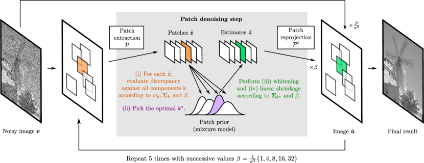
Figure 2: Illustration of EPLL framework for image denoising with a GMM prior. A large collection of (overlapping) patches are first extracted. For each patch, an optimal Gaussian component is picked based on a measure of discrepancy with the given patch. This Gaussian component is next used as a prior model to denoise the given patch by linear shrinkage in the corresponding eigenspace and depending on $\beta$. All estimated patches are finally aggregated together, weighted by $\beta$ and combined with the original noisy image to produce a first estimate. The procedure is repeated 5 times with increasing values of $\beta$.

In this paper, we suggest using a mixture of generalized Gaussian distributions that will enable image patches to be spread over clusters that are bell shaped in some directions but can be peaky with large tails in others. While the use of GMM priors leads to piece-wise linear estimator (PLE) as a function of ${\boldsymbol{z}}$ (see [66]), our GGMM prior will lead to a piecewise non-linear shrinkage estimator.

3 Generalized Gaussian Mixture Models

In this paper, we aim to learn $K$ orthogonal transforms such that each of them can map a subset (cluster) of clean patches into independent zero-mean coefficients. Instead of assuming the coefficient distributions to be bell shaped, we consider that both the scale and the shape of these distributions may vary from one coordinate to another (within the same transform). Our motivation to assume such a highly flexible model is based on the observation illustrated in Figure 1. Given one of such transform and its corresponding cluster of patches, we have displayed the histogram of the patch coefficients for six different coordinates. It can be clearly observed that the shape of the distribution varies depending on the coordinate. Some of them are peaky with heavy tails, and, therefore, would not be faithfully captured by a Gaussian distribution, as done in EPLL [67]. By contrast, some others have a bell shape, and so would not be captured properly by a peaky and heavy tailed distribution, as done for instance by sparse models [35, 40, 2, 19, 20, 53, 58]. This shows that one cannot simultaneously decorrelate and sparsify a cluster of clean patches for all coordinates. Since some of the coordinates reveal sparsity while some others reveal Gaussianity, we propose to use a more flexible model that can capture such variations. We propose using a multi-variate zero-mean generalized Gaussian mixture model (GGMM)

(8) $$p\left({\boldsymbol{z}}\right)=\sum_{k=1}^{K}w_{k}\mathcal{G}({\boldsymbol{z}};0_{P},{\boldsymbol{\Sigma}}_{k},{\boldsymbol{\nu}}_{k})$$

where $K$ is the number of components and $w_{k}>0$ are weights such that $\sum_{k}w_{k}\!=\!1$. The notation $\mathcal{G}(0_{P},{\boldsymbol{\Sigma}},{\boldsymbol{\nu}})$ denotes the $P$-dimensional generalized Gaussian distribution (GGD) with zero-mean, covariance ${\boldsymbol{\Sigma}}\in\mathbb{R}^{P\times P}$ (symmetric positive definite) and shape parameter ${\boldsymbol{\nu}}\in\mathbb{R}^{P}$, whose expression is

(9) $$\mathcal{G}({\boldsymbol{z}};0_{P},{\boldsymbol{\Sigma}},{\boldsymbol{\nu}})=\frac{\mathcal{K}}{2|{\boldsymbol{\Sigma}}_{{\boldsymbol{\nu}}}|^{1/2}}\exp\left[-{|\!|{\boldsymbol{\Sigma}}_{{\boldsymbol{\nu}}}^{-1/2}{\boldsymbol{z}}|\!|_{{\boldsymbol{\nu}}}^{{\boldsymbol{\nu}}}}\right]\quad\text{with}\quad|\!|{\boldsymbol{x}}|\!|_{{\boldsymbol{\nu}}}^{{\boldsymbol{\nu}}}=\sum_{j=1}^{P}|x_{j}|^{\nu_{j}},$$

(10) where $$\mathcal{K}=\prod_{j=1}^{P}\frac{\nu_{j}}{\Gamma(1/\nu_{j})}\quad\text{and}\quad{\boldsymbol{\Sigma}}_{{\boldsymbol{\nu}}}^{1/2}={\boldsymbol{\Sigma}}^{1/2}\begin{pmatrix}\sqrt{\frac{\Gamma(1/\nu_{1})}{\Gamma(3/\nu_{1})}}\\ &\ddots\\ &&\sqrt{\frac{\Gamma(1/\nu_{P})}{\Gamma(3/\nu_{P})}}\end{pmatrix}.$$

Denoting the eigen decomposition of matrix ${\boldsymbol{\Sigma}}$ by ${\boldsymbol{\Sigma}}={\boldsymbol{U}}{\boldsymbol{\Lambda}}{\boldsymbol{U}}^{t}$ such that ${\boldsymbol{U}}\in\mathbb{R}^{P\times P}$ is unitary and ${\boldsymbol{\Lambda}}=\operatorname{diag}(\lambda_{1},\lambda_{2},\ldots,\lambda_{P})^{2}$ is diagonal with positive diagonal elements $\lambda_{j}^{2}$, ${\boldsymbol{\Sigma}}^{1/2}$ in the above expression is defined as ${\boldsymbol{\Sigma}}^{1/2}={\boldsymbol{U}}{\boldsymbol{\Lambda}}^{1/2}$ and ${\boldsymbol{\Sigma}}^{-1/2}={\boldsymbol{\Lambda}}^{-1/2}{\boldsymbol{U}}^{t}$ is its inverse.

When ${\boldsymbol{\nu}}$ is a constant vector with all entries equal to $\nu_{j}=2$, $\mathcal{G}(0_{P},{\boldsymbol{\Sigma}},{\boldsymbol{\nu}})$ is the multi-variate Gaussian distribution $\mathcal{N}(0_{P},{\boldsymbol{\Sigma}})$ (as used in EPLL [67]). When all $\nu_{j}=1$, it is the multi-variate Laplacian distribution and the subsequent GGMM is a Laplacian Mixture Model (LMM). When all $\nu_{j}<1$, it is the multi-variate hyper-Laplacian distribution and the subsequent GGMM is a hyper-Laplacian Mixture Model (HLMM). Choosing $K=1$ with a constant vector ${\boldsymbol{\nu}}$ corresponds to $\ell_{\nu}$ regularization [20, 53]. But as motivated earlier, unlike classical multivariate GGD models [6, 47, 44], we allow for the entries of ${\boldsymbol{\nu}}$ to vary from one coordinate $j$ to another. To the best of our knowledge, the proposed work is the first one to consider this fully flexible model.

Proposition 1.

The multi-variate zero-mean GGD can be decomposed as

(11) $$\mathcal{G}({\boldsymbol{z}};0_{P},{\boldsymbol{\Sigma}},{\boldsymbol{\nu}})=\prod_{j=1}^{P}\mathcal{G}(({\boldsymbol{U}}^{t}{\boldsymbol{z}})_{j};0,\lambda_{j},\nu_{j})$$

where, for ${\boldsymbol{x}}={\boldsymbol{U}}^{t}{\boldsymbol{z}}$, the distribution of each of its components is given as

$$\mathcal{G}(x;0,\lambda,\nu)=\frac{\kappa}{2\lambda_{\nu}}\exp\left[-\left(\frac{|x|}{\lambda_{\nu}}\right)^{\nu}\right]$$

where $$\kappa=\frac{\nu}{\Gamma(1/\nu)}\quad\text{and}\quad\lambda_{\nu}=\lambda\sqrt{\frac{\Gamma(1/\nu)}{\Gamma(3/\nu)}}~{},$$

where $x\mapsto\mathcal{G}(x;0,\lambda,\nu)$ is a real, even, unimodal, bounded and continuous probability density function. It is also differentiable everywhere except for $x=0$ when $\nu\leqslant 1$.

The proof follows directly by injecting the eigen decomposition of ${\boldsymbol{\Sigma}}$ in (9) and basic properties of $x\mapsto|x|^{\nu}$. 1 shows that, for each of the $K$ clusters, eq. (9), indeed, models a prior that is separable in a coordinate system obtained by applying the whitening transform ${\boldsymbol{U}}^{t}$. Not only is the prior separable for each coordinate $j$, but the shape ($\nu_{j}$) and scale ($\lambda_{j}$) of the distribution may vary.

Before detailing the usage of GGMM priors in EPLL framework, we digress briefly to explain the procedure we used for training such a mixture of generalized Gaussian distributions where different scale and shape parameters are learned for each feature dimension.

3.1 Learning GGMMs

Parameter estimation is carried out using a modified version of the Expectation-Maximization (EM) algorithm [14]. EM is an iterative algorithm that performs at each iteration two steps, namely Expectation step (E-Step) and Maximization stop (M-Step), and is known to monotonically increase the model likelihood and converge to a local optimum. For applying EM to learn a GGMM, we leverage standard strategies used for parameter estimation for GGD and/or GGMM that are reported in previous works [35, 5, 55, 3, 16, 30, 6, 39, 47, 32]. Our M-Step update for the shape parameter $\nu$ is inspired from Mallat’s strategy [35] using statistics of the first absolute and second moments of GGDs. Since this strategy uses the method of moments for $\nu$ instead of maximum likelihood estimation, we refer to this algorithm as modified EM and the M-Step as Moment step. We also noticed that shape parameters $\nu<.3$ lead to numerical issues and $\nu>2$ leads to local minima with several degenerate components. For this reason, at each step, we impose the constraint that the learned shape parameters satisfy $\nu\in[.3,2]$. This observation is consistent with earlier works that have attempted to learn GGMM shape parameters from data [51]. Given $n$ training clean patches of size $P$ and an initialization for the $K$ parameters $w_{k}>0$, ${\boldsymbol{\Sigma}}_{k}\in\mathbb{R}^{P\times P}$ and ${\boldsymbol{\nu}}_{k}\in\mathbb{R}^{P}$, for $k=1,\ldots,K$, our modified EM algorithm iteratively alternates between the following two steps:

• Expectation step (E-Step)

  • For all components $k=1,\ldots,K$ and training samples $i=1,\ldots,n$, compute:

    $$\xi_{k,i}\leftarrow\frac{w_{k}\mathcal{G}({\boldsymbol{z}}_{i};0_{P},{\boldsymbol{\Sigma}}_{k},{\boldsymbol{\nu}}_{k})}{\sum_{l=1}^{K}w_{l}\mathcal{G}({\boldsymbol{z}}_{i};0_{P},{\boldsymbol{\Sigma}}_{l},{\boldsymbol{\nu}}_{l})}~{}.$$

• Moment step (M-Step)

  • For all components $k=1,\ldots,K$, update:

    $$w_{k} \leftarrow\frac{\sum_{i=1}^{n}\xi_{k,i}}{\sum_{l=1}^{K}\sum_{i=1}^{n}\xi_{l,i}}\quad\text{and}\quad{\boldsymbol{\Sigma}}_{k}\leftarrow\frac{\sum_{i=1}^{n}\xi_{k,i}{\boldsymbol{z}}_{i}{\boldsymbol{z}}_{i}^{t}}{\sum_{i=1}^{n}\xi_{k,i}}~{}.$$

  • Perform eigen decomposition of ${\boldsymbol{\Sigma}}_{k}$:

    $${\boldsymbol{\Sigma}}_{k}={\boldsymbol{U}}_{\!k}{\boldsymbol{\Lambda}}_{k}{\boldsymbol{U}}_{\!k}^{t}\mbox{ \quad where \quad}{\boldsymbol{\Lambda}}_{k}=\operatorname{diag}(\lambda_{k,1},\lambda_{k,2},\ldots,\lambda_{k,P})^{2}~{}.$$

  • For all components $k=1,\ldots,K$ and dimensions $j=1,\ldots,P$, compute:

    $$\chi_{k,j} \leftarrow\frac{\sum_{i=1}^{n}\xi_{k,i}|({\boldsymbol{U}}_{\!k}^{t}{\boldsymbol{z}}_{i})_{j}|}{\sum_{i=1}^{n}\xi_{k,i}}\quad\text{and}\quad({\boldsymbol{\nu}}_{k})_{j}\leftarrow\Pi_{[.3,2]}\left[F^{-1}\left(\frac{\chi_{k,j}^{2}}{\lambda_{k,j}^{2}}\right)\right]~{}.$$

where $\Pi_{[a,b]}[x]=\min(\max(x,a),b)$ and $F(x)=\frac{\Gamma(2/x)^{2}}{\Gamma(3/x)\Gamma(1/x)}$ is a monotonic invertible function that was introduced in [35] (we used a lookup table to perform its inversion as done in [5, 55]). Note that $\chi_{k,j}^{2}$ and $\lambda_{k,j}^{2}$ corresponds to the first absolute and second moments for component $k$ and dimension $j$, respectively.

For consistency purposes, we keep the training data and the number of mixture components in the models the same as that used in the original EPLL algorithm [67]. Specifically, we train our models on $n=2$ million clean patches randomly extracted from Berkeley Segmentation Dataset (BSDS) [36]. We learn $K=200$ zero-mean generalized Gaussian mixture components from patches of size $P=8\times 8$. We opted for a warm-start training by initializing our GGMM model with the GMM model from [67] and with initial values of shape parameters as 2. We run our modified EM algorithm for 100 iterations. As observed in Figure 1, the obtained GGMM models the underlying distributions of a cluster of clean patches much better than a GMM. In addition, we will see in Section 6 that our GGMM estimation did not lead to overfitting as it is also a better fit than a GMM for unseen clean patches.

3.2 Patch denoising with GGMM priors

We now explain why solving step (5) in EPLL is non-trivial when using a GGMM patch prior. In this case, for a noisy patch $\tilde{\boldsymbol{z}}$ with variance $\sigma^{2}$, equation (5) becomes

(12) $$\hat{\boldsymbol{z}} \leftarrow\underset{{\boldsymbol{z}}\in\mathbb{R}^{P}}{\operatorname{argmin}}\;\frac{1}{2\sigma^{2}}|\!|\tilde{\boldsymbol{z}}-{\boldsymbol{z}}|\!|^{2}-\log\left[\sum_{k=1}^{K}w_{k}\mathcal{G}({\boldsymbol{z}};0_{P},{\boldsymbol{\Sigma}}_{k},{\boldsymbol{\nu}}_{k})\right]~{}.$$

As for GMMs, due to the multi-modality of the GGMM prior, this optimization problem is highly non-convex. To circumvent this issue, we follow the strategy used by EPLL [67] in the specific case of Gaussian mixture model prior. The idea is to restrict the sum involved in the logarithm in eq. (12) to only one component $k^{\star}$.

If we consider the best $k^{\star}$ to be given (the strategy to select the best $k^{\star}$ will be discussed next), then eq. (12) is approximated by the following simpler problem

(13) $$\hat{\boldsymbol{z}}\leftarrow\underset{{\boldsymbol{z}}\in\mathbb{R}^{P}}{\operatorname{argmin}}\;\left\{\frac{|\!|\tilde{\boldsymbol{z}}-{\boldsymbol{z}}|\!|^{2}}{2\sigma^{2}}-\log\mathcal{G}({\boldsymbol{z}};0_{P},{\boldsymbol{\Sigma}}_{k^{\star}},{\boldsymbol{\nu}}_{k^{\star}})=\frac{|\!|\tilde{\boldsymbol{z}}-{\boldsymbol{z}}|\!|^{2}}{2\sigma^{2}}+|\!|{\boldsymbol{\Sigma}}_{{\boldsymbol{\nu}}_{k^{\star}}}^{-1/2}{\boldsymbol{z}}|\!|_{\nu}^{\nu}\right\}~{}.$$

The main advantage of this simplified version is that, by virtue of 1, the underlying optimization becomes tractable and can be separated into $P$ one-dimensional optimization problems, as:

(14) $$\hat{\boldsymbol{z}}={\boldsymbol{U}}_{\!k^{\star}}\hat{\boldsymbol{x}}\quad\text{where}\quad\hat{x}_{j}=s(\tilde{x}_{j};\sigma,\lambda_{k^{\star},j},\nu_{k^{\star},j})\quad\text{with}\quad\tilde{\boldsymbol{x}}={\boldsymbol{U}}_{\!k^{\star}}^{t}\tilde{\boldsymbol{z}}$$

(15) and $$s(x;\sigma,\lambda,\nu)=s_{\sigma,\lambda}^{\nu}(x)\in\underset{t\in\mathbb{R}}{\operatorname{argmin}}\;\frac{1}{2\sigma^{2}}(x-t)^{2}+\frac{|t|^{\nu}}{\lambda_{\nu}^{\nu}}\quad\text{where}\quad\lambda_{\nu}=\lambda\sqrt{\frac{\Gamma(1/\nu)}{\Gamma(3/\nu)}}~{},$$

where for all $k$, $\nu_{k,j}=({\boldsymbol{\nu}}_{k})_{j}$ and $\lambda_{k,j}=({\boldsymbol{\lambda}}_{k})_{j}$. While the problem is not necessarily convex, its solution $s_{\sigma,\lambda}^{\nu}$ is always uniquely defined almost everywhere (see, Section 5). We call this almost everywhere real function $s_{\sigma,\lambda}^{\nu}:\mathbb{R}\to\mathbb{R}$ shrinkage function. When $\nu=2$, it is a linear function that is often referred to as Wiener shrinkage. When $\nu\neq 2$, as we will discuss in Section 5, it is a non-linear shrinkage function that can be computed in closed form for some cases or with some approximations.

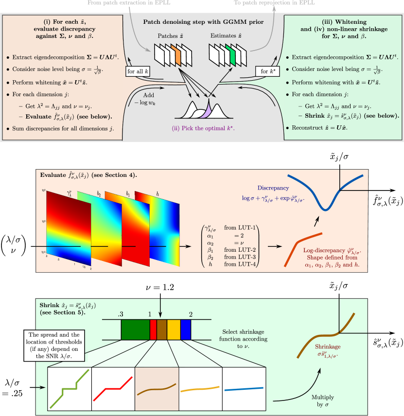
Figure 3: Illustration of our extension of EPLL to GGMM priors. The general procedure, illustrated in the top row, is similar to the original EPLL scheme described in Figure 2 but relies on generalized Gaussian distributions instead of Gaussian distributions. The shape of the discrepancy function, illustrated in the second row, depends on the given scale and shape parameters ($\lambda$ and $\nu$) of the GGD components. In Section 4, we will see that it can be approximated based on six parameters, four of them retrieved from lookup tables (LUTs). Finally, the shrinkage function, illustrated in the bottom row, can be non-linear and depends on the selected GGD component. In Section 5, we will see that it can be approximated by one of five predefined parametric functions depending on the range in which the scale parameter $\nu$ lies. The values $\nu=1.2$ and $\lambda/\sigma=.25$, shown in the bottom row, were chosen for the sake of illustration.

Now, we address the question of finding a strategy for choosing a relevant component $k^{\star}$ to replace the mixture distribution inside the logarithm. The optimal component $k^{\star}$ can be obtained by maximizing the posterior as

(16) $$k^{\star} \in\underset{1\leqslant k\leqslant K}{\operatorname{argmax}}\;p(k\;|\;\tilde{\boldsymbol{z}})=\underset{1\leqslant k\leqslant K}{\operatorname{argmax}}\;w_{k}p(\tilde{\boldsymbol{z}}\;|\;k)=\underset{1\leqslant k\leqslant K}{\operatorname{argmin}}\;-\log w_{k}-\log p(\tilde{\boldsymbol{z}}\;|\;k)$$

where the weights of the GGMM corresponds to the prior probability $w_{k}=p(k)$. We next use the fact that the patch $\tilde{\boldsymbol{z}}$ (conditioned on $k$) can be expressed as $\tilde{\boldsymbol{z}}={\boldsymbol{z}}+{\boldsymbol{n}}$ where ${\boldsymbol{z}}$ and ${\boldsymbol{n}}$ are two independent random variables from distributions $\mathcal{G}(0_{P},{\boldsymbol{\Sigma}}_{k},{\boldsymbol{\nu}}_{k})$ and $\mathcal{N}(0_{P},\sigma^{2}\boldsymbol{\mathrm{Id}}_{P})$ respectively. It follows that the distribution of $\tilde{\boldsymbol{z}}$ is the convolution of these latter two, and then

(17) $$-\log p(\tilde{\boldsymbol{z}}\;|\;k)=-\log\int_{\mathbb{R}^{P}}\mathcal{G}(\tilde{\boldsymbol{z}}-{\boldsymbol{z}};0_{P},{\boldsymbol{\Sigma}}_{k},{\boldsymbol{\nu}}_{k})\cdot\mathcal{N}({\boldsymbol{z}};0_{P},\sigma^{2}\boldsymbol{\mathrm{Id}}_{P})\;\mathrm{d}{\boldsymbol{z}}~{}.$$

We next use 1 to separate this integration problem into $P$ one-dimensional integration problems. We obtain

(18) $$-\log p(\tilde{\boldsymbol{z}}\;|\;k)=\sum_{j=1}^{P}f(({\boldsymbol{U}}_{\!k}^{t}\tilde{\boldsymbol{z}})_{j};\sigma,\lambda_{k,j},\nu_{k,j})$$

where, for $\tilde{\boldsymbol{x}}={\boldsymbol{U}}_{\!k}^{t}\tilde{\boldsymbol{z}}$, the integration problem of each of its components reads as

(19) $$f(x;\sigma,\lambda,\nu)=f_{\sigma,\lambda}^{\nu}(x)=-\log\int_{\mathbb{R}}\mathcal{G}(x-t;0,\lambda,\nu)\cdot\mathcal{N}(t;0,\sigma^{2})\;\mathrm{d}t~{}.$$

We call the real function $f_{\sigma,\lambda}^{\nu}:\mathbb{R}\to\mathbb{R}$ the discrepancy function which measures the goodness of fit of a GGD to the noisy value $x$. When $\nu=2$, this function is quadratic with $x$. For $\nu\neq 2$, as we will discuss in Section 4, it is a non-quadratic function, that can be efficiently approximated based on an in-depth analysis of its asymptotic behavior.

Figure 3 illustrates the details of the patch denoising step under the GGMM-EPLL framework. It shows that the method relies on fast approximations $\hat{f}_{\sigma,\lambda}^{\nu}$ and $\hat{s}_{\sigma,\lambda}^{\nu}$ of the discrepancy and shrinkage functions, respectively.

The next two sections are dedicated to the analysis and approximations of the discrepancy function $f_{\sigma,\lambda}^{\nu}$ and the shrinkage function $s_{\sigma,\lambda}^{\nu}$, respectively.

4 Discrepancy function: analysis and approximations

From its definition given in eq. (19), the discrepancy function reads for $\nu>0$, $\sigma>0$ and $\lambda>0$, as

(20) $$f_{\sigma,\lambda}^{\nu}(x)= -\log\frac{1}{\sqrt{2\pi}\sigma}\frac{\nu}{2\lambda_{\nu}\Gamma(1/\nu)}-\log\int_{-\infty}^{\infty}\exp\left(-\frac{(x-t)^{2}}{2\sigma^{2}}\right)\exp\left[-\left(\frac{|t|}{\lambda_{\nu}}\right)^{\nu}\right]\;\mathrm{d}t~{}.$$

It corresponds to the negative logarithm of the distribution of the sum of a zero-mean generalized Gaussian and a zero-mean Gaussian random variables. When $\nu=2$, the generalized Gaussian random variable becomes Gaussian, and the resulting distribution is also Gaussian with zero-mean and variance $\sigma^{2}+\lambda^{2}$, and then

(21) $$f_{\sigma,\lambda}^{2}(x)=\frac{1}{2}\left[\log 2\pi+\log(\sigma^{2}+\lambda^{2})+\frac{x^{2}}{\sigma^{2}+\lambda^{2}}\right]~{}.$$

Remark 1.

For $\nu=2$, a direct consequence of (21) is that $-\log p(\tilde{\boldsymbol{z}}\;|\;k)$ is as an affine function of the Mahanalobis distance between $\tilde{\boldsymbol{z}}$ and $0_{P}$ for the covariance matrix ${\boldsymbol{\Sigma}}_{k}+\sigma^{2}\boldsymbol{\mathrm{Id}}_{P}$:

(22) $$-\log p(\tilde{\boldsymbol{z}}\;|\;k)=\frac{1}{2}\left[P\log 2\pi+\log|{\boldsymbol{\Sigma}}_{k}+\sigma^{2}\boldsymbol{\mathrm{Id}}_{P}|+\tilde{\boldsymbol{z}}^{t}({\boldsymbol{\Sigma}}_{k}+\sigma^{2}\boldsymbol{\mathrm{Id}}_{P})^{-1}\tilde{\boldsymbol{z}}\right]~{}.$$

When $\nu=1$, the generalized Gaussian random variable becomes Laplacian, and the distribution resulting from the convolution also has a closed form which leads to the following discrepancy function

(23) $$f_{\sigma,\lambda}^{1}(x) =\log(2\sqrt{2}\lambda)-\frac{\sigma^{2}}{\lambda^{2}}-\log\left[e^{\frac{\sqrt{2}x}{\lambda}}\operatorname{erfc}\left(\frac{x}{\sqrt{2}\sigma}+\frac{\sigma}{\lambda}\right)+e^{-\frac{\sqrt{2}x}{\lambda}}\operatorname{erfc}\left(-\frac{x}{\sqrt{2}\sigma}+\frac{\sigma}{\lambda}\right)\right]~{},$$

refer to Appendix A for derivation (note that this expression is given in [22]).

To the best of our knowledge, there are no simple expressions for other values of $\nu$. One solution proposed by [57] is to express this in terms of the bi-variate Fox-H function [38]. This, rather cumbersome expression, is computationally demanding. In practice, this special function requires numerical integration techniques over complex lines [48], and is thus difficult to numerically evaluate it efficiently. Since, in our application, we need to evaluate this function a large number of times, we cannot utilize this solution.

In [57], the authors have also proposed to approximate this non-trivial distribution by another GGD. For fixed values of $\sigma$, $\lambda$ and $\nu$, they proposed three different numerical techniques to estimate its parameters $\lambda^{\prime}$ and $\nu^{\prime}$ that best approximate either the kurtosis, the tail or the cumulative distribution function. Based on their approach, the discrepancy function $f_{\sigma,\lambda}^{\nu}(x)$ would thus be a power function of the form $|x|^{\nu^{\prime}}$.

In this paper, we show that $f_{\sigma,\lambda}^{\nu}$ does, indeed, asymptotically behave as a power function for small and large values of $x$, but the exponent can be quite different for these two asymptotics. We believe that these different behaviors are important to be preserved in our application context. For this reason, $f_{\sigma,\lambda}^{\nu}$ cannot be modeled as a power function through a GGD distribution. Instead, we provide an alternative solution that is able to capture the correct behavior for both of these asymptotics, and that also permits fast computation.

4.1 Theoretical analysis

In this section, we perform a thorough theoretical analysis of the discrepancy function, in order to approximate it accurately. Let us first introduce some basic properties regarding the discrepancy function.

Proposition 2.

Let $\nu>0$, $\sigma>0$, $\lambda>0$ and $f_{\sigma,\lambda}^{\nu}$ as defined in eq. (19). The following relations hold true

(reduction) $$f_{\sigma,\lambda}^{\nu}(x) =\log\sigma+f_{1,\lambda/\sigma}^{\nu}(x/\sigma)~{},$$

(even) $$f_{\sigma,\lambda}^{\nu}(x) =f_{\sigma,\lambda}^{\nu}(-x)~{},$$

(unimodality) $$|x|\geqslant|y| \Leftrightarrow f_{\sigma,\lambda}^{\nu}(|x|)\geqslant f_{\sigma,\lambda}^{\nu}(|y|)~{},$$

(lower bound at 0) $$\min_{x\in\mathbb{R}}f_{\sigma,\lambda}^{\nu}(x) =f_{\sigma,\lambda}^{\nu}(0)>-\infty~{}.$$

The proofs can be found in Appendix B. Based on 2, we can now express the discrepancy function $f_{\sigma,\lambda}^{\nu}(x):\mathbb{R}\to\mathbb{R}$ in terms of a constant $\gamma_{\lambda}^{\nu}$ and another function $\varphi_{\lambda}^{\nu}:\mathbb{R}_{+}^{*}\to\mathbb{R}$, both of which can be parameterized by only two parameters $\lambda>0$ and $\nu>0$, as

(26) $$f_{\sigma,\lambda}^{\nu}(x) =\log\sigma+\gamma_{\lambda/\sigma}^{\nu}+\left\{\begin{array}[]{ll}e^{\varphi_{\lambda/\sigma}^{\nu}(|x/\sigma|)}&\text{if}\quad x\neq 0~{},\\ 0&\text{otherwise}~{},\end{array}\right.$$

(27) $$\quad\text{where}\quad\varphi_{\lambda}^{\nu}(x) =\log\left[f_{1,\lambda}^{\nu}(x)-\gamma_{\lambda}^{\nu}\right]\quad\text{and}\quad\gamma_{\lambda}^{\nu}=f_{1,\lambda}^{\nu}(0)~{}.$$

We call $\varphi_{\lambda}^{\nu}$ the log-discrepancy function.

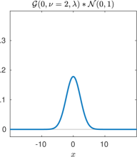
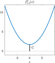
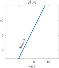
Figure 4: From left to right: the convolution of a Gaussian distribution with standard deviation $\lambda=2$ with a Gaussian distribution with standard deviation $\sigma=1$, the corresponding discrepancy function and log-discrepancy function.

At this point, let us consider an instructive toy example for the case when $\nu=2$. In this case, from eq. (21), we can deduce that the log-discrepancy function is a log-linear function (i.e., a linear function of $\log x$)

(28) $$\varphi^{2}_{\lambda}(x)=\alpha\log x+\beta~{},$$

(29) and $$\gamma^{2}_{\lambda}=\tfrac{1}{2}\left[\log 2\pi+\log(1+\lambda^{2})\right]~{},$$

(30) where $$\alpha=2\quad\text{and}\quad\beta=-\log 2-\log(1+\lambda^{2})~{}.$$

Here, the slope $\alpha=2$ reveals the quadratic behavior of the discrepancy function. Figure 4 gives an illustration of the resulting convolution (a Gaussian distribution), the discrepancy function (a quadratic function) and the log-discrepancy (a linear function with slope $2$). Note that quadratic metrics are well-known to be non-robust to outliers, which is in complete agreement with the fact that Gaussian priors have thin tails.

Another example is the case of $\nu=1$. From eq. (23), the log-discrepancy is given by

(31) $$\varphi^{1}_{\lambda}(x) =\log\left[\log\left[2\operatorname{erfc}{\left(\textstyle\frac{1}{\lambda}\right)}\right]-\log\left[e^{\frac{\sqrt{2}x}{\lambda}}\operatorname{erfc}{\left(\textstyle\frac{x}{\sqrt{2}}+\frac{1}{\lambda}\right)}+e^{-\frac{\sqrt{2}x}{\lambda}}\operatorname{erfc}{\left(\textstyle-\frac{x}{\sqrt{2}}+\frac{1}{\lambda}\right)}\right]\right]~{},$$

(32) and $$\gamma_{\lambda}^{1}=\frac{1}{2}\log 2+\log\lambda-\frac{1}{\lambda^{2}}-\log\left[\operatorname{erfc}{\left(\textstyle\frac{1}{\lambda}\right)}\right]~{}.$$

Unlike for $\nu=2$, this function is not log-linear and thus $f_{\sigma,\lambda}^{1}$ is not a power function. Nevertheless, as shown by the next two theorems, it is also asymptotically log-linear for small and large values of $x$.

Theorem 1.

The function $\varphi_{\lambda}^{1}$ is asymptotically log-linear in the vicinity of $0$

(33) $$\varphi_{\lambda}^{1}(x)\underset{0}{\sim}\;\alpha_{1}\log x+\beta_{1}~{},$$

(34) where $$\alpha_{1}=2\quad\text{and}\quad\beta_{1}=-\log\lambda+\log\left[\frac{1}{\sqrt{\pi}}\frac{\exp\left(-\frac{1}{\lambda^{2}}\right)}{\operatorname{erfc}\left(\frac{1}{\lambda}\right)}-\frac{1}{\lambda}\right]~{}.$$

The proof can be found in Appendix C.

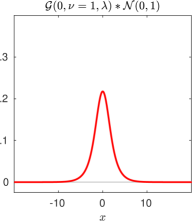
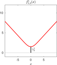
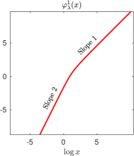
Figure 5: From left to right: the convolution of a Laplacian distribution with standard deviation $\lambda=2$ with a Gaussian distribution with standard deviation $\sigma=1$, the corresponding discrepancy function and log-discrepancy function.

Theorem 2.

The function $\varphi_{\lambda}^{1}$ is asymptotically log-linear in the vicinity of $+\infty$

(35) $$\varphi_{\lambda}^{1}(x)\underset{\infty}{\sim}\;\alpha_{2}\log x+\beta_{2}~{},$$

(36) where $$\alpha_{2}=1\quad\text{and}\quad\beta_{2}=\frac{1}{2}\log 2-\log\lambda~{}.$$

The proof can be found in Appendix D.

1 and 2 show that $\varphi_{\lambda}^{1}$ has two different asymptotics that can be approximated by a log-linear function. Interestingly, the exponent $\alpha_{1}=2$ in the vicinity of $0$ shows that the Gaussian distribution involved in the convolution prevails over the Laplacian distribution and thus, the behavior of $f_{\sigma,\lambda}^{1}$ is quadratic. Similarly, the exponent $\alpha_{2}=1$ in the vicinity of $+\infty$ shows that the Laplacian distribution involved in the convolution prevails over the Gaussian distribution and the behavior of $f_{\sigma,\lambda}^{1}$ is then linear. These results are supported by Figure 5 which illustrates the resulting convolution, the discrepancy function (eq. (23)) and the log-discrepancy function (eq. (31)). Furthermore, the discrepancy function $f_{\sigma,\lambda}^{1}$ shares a similar behavior with the well-known Huber loss function [28] (also called smoothed $\ell_{1}$), known to be more robust to outliers. This is again in complete agreement with the fact that Laplacian priors have heavier tails.

In the case $\frac{2}{3}<\nu<2$, even though $\varphi_{\lambda}^{\nu}$ has no simple closed form expression, the similar conclusions can be made as a result of the next two theorems.

Theorem 3.

Let $\nu>0$. The function $\varphi^{\nu}_{\lambda}$ is asymptotically log-linear in the vicinity of $0$

$$\varphi^{\nu}_{\lambda}(x)\underset{0}{\sim}\;\alpha_{1}\log x+\beta_{1}~{},$$

where $$\alpha_{1}=2\quad\text{and}\quad\beta_{1}=-\log 2+\log\left(1-\frac{\displaystyle\int_{-\infty}^{\infty}t^{2}e^{-\frac{t^{2}}{2}}\exp\left[-\left(\frac{|t|}{\lambda_{\nu}}\right)^{\nu}\right]\;\mathrm{d}t}{\displaystyle\int_{-\infty}^{\infty}e^{-\frac{t^{2}}{2}}\exp\left[-\left(\frac{|t|}{\lambda_{\nu}}\right)^{\nu}\right]\;\mathrm{d}t}\right)~{}.$$

The proof can be found in Appendix E.

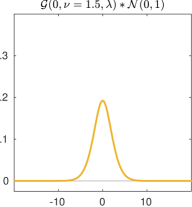
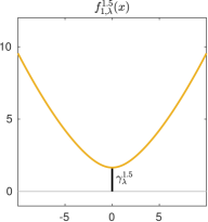
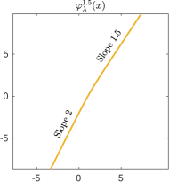
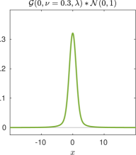
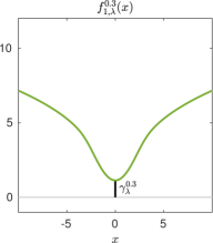
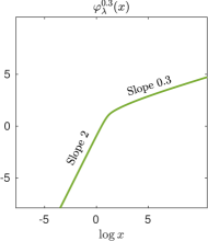
Figure 6: From left to right: the convolution of a generalized Gaussian distribution with standard deviation $\lambda=2$ with a Gaussian distribution with standard deviation $\sigma=1$, the corresponding discrepancy function and log-discrepancy function. From top to bottom: the GGD has a shape parameter $\nu=1.5$ and $.3$, respectively.

Theorem 4.

Let $\frac{2}{3}<\nu<2$, then $\varphi^{\nu}_{\lambda}$ is asymptotically log-linear in the vicinity of $+\infty$

$$\varphi^{\nu}_{\lambda}(x)\underset{\infty}{\sim}\;\alpha_{2}\log x+\beta_{2}~{},$$

where $$\alpha_{2}=\nu\quad\text{and}\quad\beta_{2}=-\nu\log\lambda-\frac{\nu}{2}\log\frac{\Gamma(1/\nu)}{\Gamma(3/\nu)}~{}.$$

The proof relies on a result of Berman (1992) [4] and is detailed in Appendix F.

Remark 2.

For $\nu>2$, an asymptotic log-linear behavior with $\alpha_{2}=2$ and $\beta_{2}=-\log 2$ can be obtained using exactly the same sketch of proof as the one of 4.

Remark 3.

For $\nu=2$, we have $\varphi_{\lambda}^{2}$ is linear, $\beta_{1}=-\log 2-\log\left(1+\lambda^{2}\right)$ and $\beta_{2}=-\log 2-\log\lambda^{2}$, which shows that 4 cannot hold true for $\nu=2$.

Remark 4.

For $\nu=1$, 1 and 2 coincide with 3 and 4.

Remark 5.

For $0<\nu\leqslant\frac{2}{3}$, though we did not succeed in proving it, our numerical simulations also revealed a log-linear asymptotic behavior for $x\to\infty$ in perfect agreement with the expression of $\alpha_{2}$ and $\beta_{2}$ given in 4.

Again, the exponent $\alpha_{1}=2$ in the vicinity of $0$ shows that the Gaussian distribution involved in the convolution prevails over the generalized Gaussian distribution and the behavior of $f_{\sigma,\lambda}^{\nu}$ is then quadratic. Similarly, the exponent $\alpha_{2}=\nu$ in the vicinity of $+\infty$ shows that the generalized Gaussian distribution involved in the convolution prevails over the Gaussian distribution and the behavior of $f_{\sigma,\lambda}^{\nu}$ is then a power function of the form $x^{\nu}$. These results are supported by Figure 6 that illustrates the resulting convolution, the discrepancy function and the log-discrepancy function for $\nu=1.5$ and $\nu=.3$. Moreover, the discrepancy function $f_{\sigma,\lambda}^{\nu}$ with $\nu\leqslant 1$ shares a similar behavior with well-known robust M-estimator loss functions [27]. In particular, the asymptotic case for $\nu\to 0$ resembles the Tukey’s bisquare loss, known to be insensitive to outliers. This is again in complete agreement with GGD priors having larger tails as $\nu$ goes to $0$.

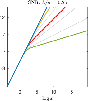
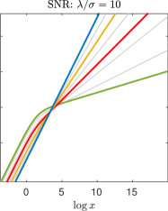
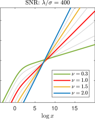
Figure 7: Illustrations of the log-discrepancy function for various $0.3\leqslant\nu\leqslant 2$ and SNR $\lambda/\sigma$.

Figure 7 shows the evolution of the log-discrepancy function for various values of $\nu$ in the context of three different signal-to-noise ratios $\lambda/\sigma$ (SNR). One can observe that as the SNR decreases (resp., increases), the left (resp., right) asymptotic behavior starts dominating over the right (resp., left) asymptotes. In other words, for $\nu<2$, the intersection of the two asymptotes goes to $+\infty$ (resp., $-\infty$). Last but not least, for $0<\nu\leqslant 2$, the log-discrepancy function $\varphi_{\lambda}^{\nu}$ is always concave and since $\alpha_{2}\leqslant\alpha_{1}$ it is thus upper-bounded by its left and right asymptotes.

From 3, 4 and 5, we can now build two asymptotic log-linear approximations for $\varphi_{\lambda}^{\nu}$, with $0<\nu\leqslant 2$, and subsequently an asymptotic power approximation for $f_{\sigma,\lambda}^{\nu}$ by using the relation (26). Next, we explain the approximation process of the in-between behavior, as well as its efficient evaluation.

4.2 Numerical approximation

We now describe the proposed approximation of the discrepancy function $f_{1,\lambda}^{\nu}$ through an approximation $\hat{\varphi}_{\lambda}^{\nu}$ of the log-discrepancy function as

(37) $$\hat{f}_{1,\lambda}^{\nu}(x)=\gamma_{\lambda}^{\nu}+\exp\hat{\varphi}_{\lambda}^{\nu}(x)\quad\text{where}\quad\gamma_{\lambda}^{\nu}=f_{1,\lambda}^{\nu}(0)~{}.$$

Based on our previous theoretical analysis, a solution preserving the asymptotic, increasing and concave behaviors of $\varphi_{1,\lambda}^{\nu}$ can be defined by making use of the following approximations

(38) $$\hat{\varphi}_{\lambda}^{\nu}(x)=\alpha_{1}\log|x|+\beta_{1}-\texttt{rec}(\alpha_{1}\log|x|+\beta_{1}-\alpha_{2}\log|x|-\beta_{2})~{},$$

where rec is a so-called rectifier function that is positive, increasing, convex and satisfies

(39) $$\underset{x\to-\infty}{\lim}\;\texttt{rec}(x)=0~{}\quad\text{and}\quad\texttt{rec}(x)\underset{x\to\infty}{\sim}\;x~{}.$$

In this paper, we consider the two following rectifying functions

(40) $$\texttt{relu}(x)=\max(0,x)\quad\text{and}\quad\texttt{softplus}(x)=h\log\left[1+\exp\left(\frac{x}{h}\right)\right],~{}h>0~{},$$

as coined respectively in [42] and [18]. Using the function relu (Rectified linear unit) leads to an approximation $\hat{\varphi}_{\lambda}^{\nu}$ that is exactly equal to the asymptotes of $\varphi_{\lambda}^{\nu}$ with a singularity at their crossing point. In this paper, we will instead use the function softplus as it allows the approximation of $\varphi_{\lambda}^{\nu}$ to converge smoothly to the asymptotes without singularity. Its behavior is controlled by the parameter $h>0$. The smaller the value of $h$ is, the faster the convergence speed to the asymptotes.

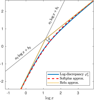
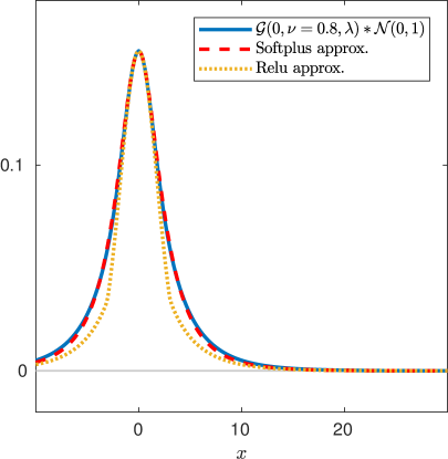
Figure 8: Illustrations of our approximations of $\varphi_{\lambda}^{\nu}$ and the corresponding underlying posterior distribution $\mathcal{N}(0,\nu,\lambda)*\mathcal{G}(0,1)$ (where $\nu=.8$ and $\lambda=4$). The blue curves have been obtained by evaluating the convolution using numerical integration techniques for all $x$. The dashed curves are obtained using the proposed relu- and softplus-based approximations that have closed-form expressions.

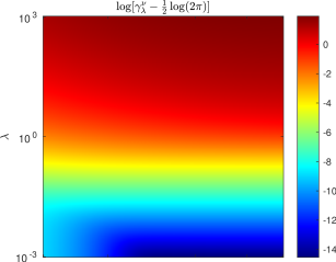
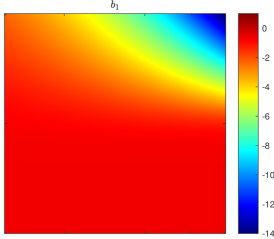
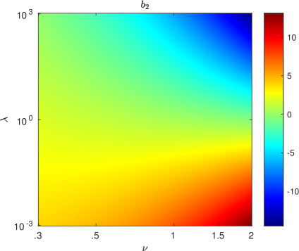
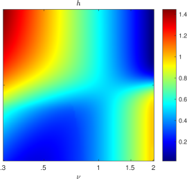
Figure 9: Lookup tables used to store the values of the parameters $\gamma_{\lambda}^{\nu}$, $\beta_{1}$, $\beta_{2}$ and $h$ for various $.3\leqslant\nu\leqslant 2$ and $10^{-3}\leqslant\lambda\leqslant 10^{3}$. A regular grid of $100$ values has been used for $\nu$ and a logarithmic grid of $100$ values has been used for $\lambda$. This leads to a total of $10,000$ combinations for each of the four lookup tables.

The parameter $h$ should be chosen such that the approximation error between $\hat{\varphi}_{\lambda}^{\nu}(x)$ and $\varphi_{\lambda}^{\nu}(x)$ is as small as possible. This can be done numerically by first evaluating $\varphi_{\lambda}^{\nu}(x)$ with integration techniques for a large range of values $x$, and then selecting the parameter $h$ by least square. Of course, the optimal value for $h$ depends on the parameter $\lambda$ and $\nu$.

Figure 8 gives an illustration of our approximations of the log-discrepancy and the corresponding distribution obtained with relu and softplus. On this figure the underlying functions have been obtained by numerical integration for a large range of value of $x$. One can observe that using softplus provides a better approximation than relu.

Our approximation for $\hat{f}_{1,\lambda}^{\nu}(x)$ is parameterized by six scalar values: $\gamma_{\nu}^{\lambda}$, $\alpha_{1}$, $\beta_{1}$, $\alpha_{2}$, $\beta_{2}$ and $h$ that depend only on the original parameters $\lambda$ and $\nu$. From our previous analysis, we have that $\alpha_{1}=2$ and $\alpha_{2}=\nu$. The other parameters are non-linear functions of $\lambda$ and $\nu$. The parameters $\gamma_{\nu}^{\lambda}$, $\beta_{1}$ and $\beta_{2}$ require either performing numerical integration or evaluating the special function $\Gamma$. As discussed, the parameter $h$ requires numerical integration for various $x$ and then optimization. For these reasons, these values cannot be computed during runtime. Instead, we pre-compute these four parameters offline for $10,000$ different combinations of $\lambda$ and $\nu$ values in the intervals $[10^{-3},10^{3}]$ and $[0.3,2]$, respectively (the choice for this range was motivated in Section 3.1). The resulting values are then stored in four corresponding lookup tables. During runtime, these parameters are retrieved online by bi-linear extrapolation and interpolation. The four lookup tables are given in Figure 9. We will see in Section 6 that using the approximation $\hat{f}_{1,\lambda}^{\nu}$ results in substantial acceleration without significant loss of performance as compared to computing $f_{1,\lambda}^{\nu}$ directly by numerical integration during runtime.

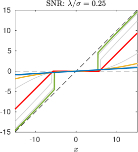
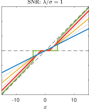
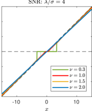
Figure 10: Illustrations of the shrinkage function for various $0.3<\nu\leqslant 2$ and SNR $\lambda/\sigma$.

5 Shrinkage functions: analysis and approximations

Recall that from its definition given in eq. (15), the shrinkage function is defined for $\nu>0$, $\sigma>0$ and $\lambda>0$, as

(41) $$s_{\sigma,\lambda}^{\nu}(x) \in\underset{t\in\mathbb{R}}{\operatorname{argmin}}\;\frac{(x-t)^{2}}{2\sigma^{2}}+\lambda_{\nu}^{-\nu}|t|^{\nu}~{}.$$

5.1 Theoretical analysis

Except for some particular values of $\nu$ (see, Section 5.2), Problem (41) does not have explicit solutions. Nevertheless, as shown in [40], Problem (41) admits two (not necessarily distinct) solutions. One of them is implicitly characterized as

(44) $$s_{\sigma,\lambda}^{\nu}(x)=\left\{\begin{array}[]{ll}0&\text{if}\quad 0<\nu\leqslant 1\quad\text{and}\quad|x|\leqslant\tau_{\lambda}^{\nu}~{},\\ t^{\star}&\text{otherwise}~{},\end{array}\right.$$

where $$t^{\star}=x-\operatorname{sign}(t^{\star})\nu\sigma^{2}\lambda_{\nu}^{-\nu}|t^{\star}|^{\nu-1}~{},$$

(47) and $$\tau_{\lambda}^{\nu}=\left\{\begin{array}[]{ll}(2-\nu)(2-2\nu)^{-\frac{1-\nu}{2-\nu}}(\sigma^{2}\lambda_{\nu}^{-\nu})^{\frac{1}{2-\nu}}&\text{if}\quad\nu<1~{},\\ \sigma^{2}\lambda^{-1}&\text{otherwise}\;\text{($\nu=1$)}~{}.\end{array}\right.$$

The other one is obtained by changing $|x|\leqslant\tau_{\lambda}^{\nu}$ to $|x|<\tau_{\lambda}^{\nu}$ in (44), and so they coincide for almost every $(x,\lambda,\sigma,\nu)$. As discussed in [40], for $\nu>1$, $s_{\sigma,\lambda}^{\nu}(x)$ is differentiable, and for $\nu\leqslant 1$, the shrinkage exhibits a threshold $\tau_{\lambda}^{\nu}$ that produces sparse solutions. 3 summarizes a few important properties.

Proposition 3.

Let $\nu>0$, $\sigma>0$, $\lambda>0$ and $s_{\sigma,\lambda}^{\nu}$ as defined in eq. (15). The following relations hold true

(reduction) $$s_{\sigma,\lambda}^{\nu}(x) =\sigma s_{1,\frac{\lambda}{\sigma}}^{\nu}\left(\frac{x}{\sigma}\right)~{},$$

(odd) $$s_{\sigma,\lambda}^{\nu}(x) =-s_{\sigma,\lambda}^{\nu}(-x)~{},$$

(50) $$s_{\sigma,\lambda}^{\nu}(x) \in\left\{\begin{array}[]{ll}{[}0,x{]}&\text{if}\quad x\geqslant 0\\ {[}x,0{]}&\text{otherwise}\\ \end{array}\right.~{},$$

(increasing with $$x x_{1}\geqslant x_{2} \Leftrightarrow s_{\sigma,\lambda}^{\nu}(x_{1})\geqslant s_{\sigma,\lambda}^{\nu}(x_{2})~{},$$)

(increasing with $$\lambda \lambda_{1}\geqslant\lambda_{2} \Leftrightarrow s_{\sigma,\lambda_{1}}^{\nu}(x)\geqslant s_{\sigma,\lambda_{2}}^{\nu}(x)~{},$$)

(kill low SNR) $$\underset{\frac{\lambda}{\sigma}\to 0}{\lim}\; s_{\sigma,\lambda}^{\nu}(x)=0~{},$$

(keep high SNR) $$\underset{\frac{\lambda}{\sigma}\to+\infty}{\lim}\; s_{\sigma,\lambda}^{\nu}(x)=x~{}.$$

The proofs can be found in Appendix G. These properties show that $s_{\sigma,\lambda}^{\nu}$ is indeed a shrinkage function (non-expansive). It shrinks the input coefficient $x$ according to the model $\nu$ and the modeled signal to noise ratio $\frac{\lambda}{\sigma}$ (SNR). When $x$ is small in comparison to the SNR, it is likely that its noise component dominates the underlying signal, and is, therefore, shrunk towards $0$. Similarly, when $x$ is large, it will likely be preserved. This is even more likely when $\nu$ is small, since in this case large coefficients are favored by the prior. Illustrations of shrinkage functions for various SNR and $\nu$ are given in Figure 10.

Table 1: Shrinkage function under generalized Gaussian priors

$\nu$	Shrinkage $s_{\sigma,\lambda}^{\nu}(x)$	Remark
$<1$	$\displaystyle\left\{\begin{array}[]{ll}\displaystyle x-\gamma x^{\nu-1}+O(x^{2(\nu-1)})&\displaystyle\text{if}\quad|x|\geqslant\tau_{\lambda}^{\nu}\\ 0&\text{otherwise}\\ \end{array}\right.$	$\begin{array}[]{r}\approx\text{Hard-thresholding}\\ \text{\cite[cite]{[\@@bibref{}{moulin1999analysis}{}{}]}}\\ \end{array}$
$1$	$\displaystyle\operatorname{sign}(x)\max\left(|x|-\frac{\sqrt{2}\sigma^{2}}{\lambda},0\right)$	$\begin{array}[]{r}\text{Soft-thresholding}\\ \text{\cite[cite]{[\@@bibref{}{donoho1994ideal}{}{}]}}\\ \end{array}$
$4/3$	$\displaystyle x+\gamma\left(\sqrt[3]{\frac{\zeta-x}{2}}-\sqrt[3]{\frac{\zeta+x}{2}}\right)$	[10]
$3/2$	$\displaystyle\operatorname{sign}(x)\frac{\left(\sqrt{\gamma^{2}+4|x|}-\gamma\right)^{2}}{4}$	[10]
$2$	$\displaystyle\frac{\lambda^{2}}{\lambda^{2}+\sigma^{2}}\cdot x$	Wiener (LMMSE)

$$\text{with}\quad\gamma=\nu\sigma^{2}\lambda_{\nu}^{-\nu}\quad\text{and}\quad\zeta=\sqrt{x^{2}+4\left(\frac{\gamma}{3}\right)^{3}}~{}.$$

 

5.2 Numerical approximations

The shrinkage function $s_{\sigma,\lambda}^{\nu}$, implicitly defined in (44) does not have a closed form expression in general. Nevertheless, for fixed values of $x$, $\sigma$, $\lambda$, $\nu$, $s_{\sigma,\lambda}^{\nu}(x)$ can be estimated using iterative solvers such as Newton descent or Halley’s root-finding method. These approaches converge quite fast and, in practice, reach a satisfying solution within ten iterations. However, since in our application of interest we need to evaluate this function a large number times, we will follow a different path in order to reduce computation time (even though we have implemented this strategy).

As discussed earlier, $s_{\sigma,\lambda}^{\nu}$ is known in closed form for some values of $\nu$, more precisely: $\nu=\{1,4/3,3/2,2\}$ (as well as $\nu=3$ but this is out of the scope of this study), see for instance [10]. When $\nu=2$, we retrieve the linear minimum mean square estimator (known in signal processing as Wiener filtering) and related to Tikhonov regularization and ridge regression. This shrinkage is linear and the slope of the shrinkage goes from $0$ to $1$ as the SNR increases (see Figure 10). When $\nu=1$, the shrinkage is the well-known soft-thresholding [17], corresponding to the maximum a posteriori estimator under a Laplacian prior. When $\nu<1$, the authors of [40] have shown that (i) the shrinkage admits a threshold with a closed-form expression (given in eq. (44)), and (ii) the shrinkage is approximately equal to hard-thresholding with an error term that vanishes when $|x|\to\infty$. All these expressions are summarized in Table 1.

In order to keep our algorithm as fast as possible, we propose to use the approximation of the shrinkage given for $\nu<1$ in [40]. Otherwise, we pick one of the four shrinkage functions corresponding to $\nu=\{1,4/3,3/2,2\}$ by nearest neighbor on the actual value of $\nu\in[1,2]$. Though this approximation may seem coarse compared to the one based on iterative solvers, we did not observe any significant loss of quality in our numerical experiments (see Section 6). Nonetheless, this alternative leads to 6 times speed-up while evaluating shrinkage.

6 Experimental evaluation

In this section we explain the methodology used to evaluate the GGMM model, and present numerical experiments to compare the performance of the proposed GGMM model over existing GMM-based image denoising algorithms. To demonstrate the advantage of allowing for a flexible GGMM model, we also present results using GGMM models with fixed shape parameters, $\nu=1$ (Laplacian mixture model) and $\nu=0.5$ (Hyper-Laplacian mixture model). For learning Laplacian mixture model (LMM) and hyper-Laplacian mixture model (HLMM), we use the same procedure as described in Section 3.1 but force all shape parameters to be equal to $1$ or $0.5$, respectively.

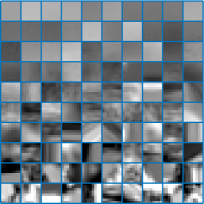
(a) GMM ($\nu=2$)

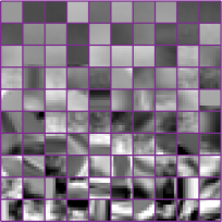
(b) GGMM ($.3\leqslant\nu\leqslant 2$)

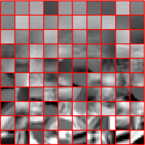
(c) LMM ($\nu=1$)

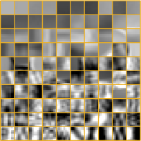
(d) HLMM ($\nu=.5$)

Figure 11: Set of 100 patches, sorted by the norm of their gradient, and generated to be independently distributed according to (from left to right) a GMM, GGMM, LMM and HLMM. For ease of visualization, only the top eigendirections corresponding to $80\%$ of the variance have been chosen. Near-constant patches with variance smaller than $\tfrac{2}{P}|\!|{\boldsymbol{\Sigma}}_{k}|\!|_{F}^{2}$ have also been discarded.

Model validation

As discussed in Section 3, Figure 1 illustrates the validity of our model choices with histograms of different dimensions of a single patch cluster. It clearly shows the importance of allowing the shape and scale parameter to vary across dimensions for capturing underlying patch distributions. Since GGMM (and obviously, GMM) falls into the class of generative models, one can also assess the expressivity of a model by analyzing the variability of generated patches and its ability to generate relevant image features (edges, texture elements etc.). This can be tested by selecting a component $k$ of the GGMM (or GMM) with probability $w_{k}$ and sampling patches from the GGD (or GD) as described in [43]. Figure 11 presents a collage of 100 patches independently generated by this procedure using GMM, GGMM, LMM and HLMM. As observed, patches generated from GGMM show greater balance between strong/faint edges, constant patches and subtle textures than the models that use constant shape parameters such as GGM, LMM and HLMM.

The superiority of our GGMM model over GMM, LMM or HLMM models can also be illustrated by comparing the log-likelihood (LL) achieved by these models over a set of clean patches from natural images. Note that, to maintain objectivity, the models have to be tested on data that is different than the dataset used during training. To this end, we compute the LL of the four above-mentioned models on all non-overlapping patches of $40$ randomly selected images extracted from BSDS testing set [36], which is a different set than the training images used in the EM algorithm (parameter estimation/model learning). One can observe that not only GGMM is a better fit than GMM, LMM and HLMM on average for the $40$ images, but it is also a better fit on each single image. Given that GGMM have a larger degree of freedom than GMM, this study proves that our learning procedure did not fall prey to over-fitting, and that the extra flexibility provided by GGMM was used to capture relevant and accurate image patterns.

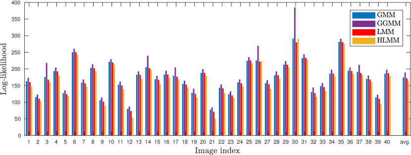
Figure 12: Average log-likelihood of all non-overlapping patches (with subtracted mean) of each of the $40$ images of our validation subset of the testing BSDS dataset for the GMM, GGMM, LMM and HLMM. The total average over the $40$ images is shown in the last column.

Denoising evaluation

Following the verification of the model, we provide a thorough evaluation of our GGMM prior in denoising task by comparing its performance against EPLL that uses a GMM prior [67] and with our LMM and HLMM models explained above. For the ease of comparison, we utilize the pipeline and settings that was prescribed for the original EPLL [67] algorithm (see Section 2.1). To reduce the computation time of all EPLL-based algorithms, we utilize the random patch overlap procedure introduced by [46]. That is, instead of extracting all patches at each iteration, a randomly selected but different subset of overlapping patches consisting of only $3\%$ of all possible patches is processed in each iteration. For the sake of reproducibility of our results, we have made our MATLAB/MEX-C implementation available online at https://bitbucket.org/cdeledalle/ggmm-epll.

The evaluation is carried out on classical images such as Barbara, Cameraman, Hill, House, Lena and Mandrill, and on 60 images taken from BSDS testing set [36] (the original BSDS test data contains 100 images, the other 40 were used for model validation experiments). All image have been corrupted independently by ten independent realizations of additive white Gaussian noise with standard deviation $\sigma=5,10,20,40$ and $60$ (with pixel values between $[0,255]$). The EPLL algorithm using mixture of Gaussian, generalized Gaussian priors are indicated as GMM and GGMM in LABEL:tab:psnr_denoising. Results obtained with BM3D algorithm [12] are also included for reference purposes. To stay with the focus of this paper, i.e., on the effect of image priors on EPLL-based algorithms, BM3D will be excluded from our performance comparison discussions. The denoising performance of the algorithms are measured in terms of Peak Signal to Noise Ratio (PSNR) and Structural SIMilarity (SSIM) [62]. As can be observed in LABEL:tab:psnr_denoising, in general, GGMM prior provides better PSNR performance than the GMM prior. In terms of SSIM values (shown in the bottom part of LABEL:tab:psnr_denoising), GGMM prior is comparable to GMM. In order to demonstrate the effect of fixed $\nu$ values compared to the more flexible GGMM prior, we compare the results of GGMM against GMM ($\nu=2$), Laplacian Mixture Model (GGMM with $\nu=1$) and hyper-Laplacian mixture model (GGMM with $\nu=0.5$) priors in the same scenarios for $\sigma=5,20$ and $60$. These results are shown in LABEL:tab:psnr_denoising_nu. GGMM prior provides better PSNR performance on average than the fixed-shape priors. The differences in denoising performance can also be verified visually in LABEL:fig:castle, LABEL:fig:cameraman and LABEL:fig:barbara. The denoised images obtained using GGMM prior show much fewer artifacts as compared to GMM-EPLL results, in particular in homogeneous regions. On the other hand, GGMM prior is also able to better preserve textures than LMM and HLMM.

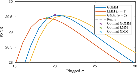
Figure 13: Evolution of performance of EPLL with a GGMM, LMM ($\nu=1$) and a GMM ($\nu=2$) under misspecification of the noise standard deviation $\sigma$. Performances are measured in terms of PSNR on the BSDS dataset corrupted by a Gaussian noise with standard deviation $\sigma=20$. For each of the three priors, EPLL has been run assuming $\sigma$ was ranging from $15$ to $30$.

Prior fitness for image denoising

In this work, we have considered non-blind image denoising. That is, the noise standard deviation is assumed to be known. In this setting, if the restoration model is accurate, one should ideally achieve optimal restoration performance when using the true degradation. To verify this, we conducted a denoising task with image corrupted with noise with standard deviation $\sigma=20$. We used GMM, LMM and GGMM priors in the restoration framework with assumed $\sigma$ values ranging from 15 to 30. Figure 13 shows the evolution of average restoration performance over 40 images from BSDS testing set (kept aside for validation, as mentioned above) with varying noise variances. GGMM prior attains its best performance when the noise variance used in the restoration model matches with the ground truth $\sigma=20$. In contrast to GGMM, GMM (resp., LMM) reaches its best performance at a larger (resp., lower) value of $\sigma$ than the correct noise used during degradation. This is because GMM tends to under-smooth clean patches (resp., over-smooth) so that a larger (resp., lower) value of $\sigma$ is required to compensate the mismatch between the assumed prior and the actual distribution in the restoration model. This indicates that GGMM is a better option to model distribution of image patches than GMM or LMM.

Influence of our approximations

All previous experiments using GGMM patch priors were conducted based on the two proposed approximations introduced in Section 4 and Section 5. In LABEL:fig:direct_vs_approx and LABEL:tab:profile, we provide a quantitative illustration of the speed-ups provided by these approximations and their effect on denoising performance. Timings were carried out with Matlab 2018a on an Intel(R) Core(TM) i7-7600U CPU @ 2.80GHz (neither multi-core paralellization nor GPUs acceleration were used). LABEL:fig:direct_vs_approxa shows the result obtained by calculating original discrepancy function via numerical integration and the shrinkage function via Halley’s root-finding method. This makes the denoising process extremely slow and takes 10 hours and 29 minutes for denoising an image of size 128$\times$128 pixels. The approximated discrepancy function provides 4 orders of magnitude speed-up with no perceivable drop in performance (LABEL:fig:direct_vs_approxb). In addition, incorporating the shrinkage approximation provides further acceleration that allows the denoising to complete in less than 2 seconds with a very minor drop in PSNR/SSIM. As indicated in the detailed profiles on LABEL:tab:profile, the shrinkage approximation provides an acceleration of six-fold to the shrinkage calculation step itself and leads to an overall speed-up of 1.5 due to the larger bottleneck caused by discrepancy function calculation. The approximately 23,000$\times$ speed-up realized without any perceivable drop in denoising performance underscores the efficacy of our proposed approximations.

7 Conclusions and Discussion

In this work, we suggest using a mixture of generalized Gaussians for modeling the patch distribution of clean images. We provide a detailed study of the challenges that one encounters when using a highly flexible GGMM prior for image restoration in place of a more common GMM prior. We identify the two main bottlenecks in the restoration procedure when using EPLL and GGMM – namely, the patch classification step and the shrinkage step. One of the main contributions of this paper, is the thorough theoretical analysis of the classification problem allowing us to introduce an asymptotically accurate approximation that is computationally efficient. In order to tackle the shrinkage step, we collate and extend the existing solutions under GGMM prior.

Our numerical experiments indicate that our flexible GGMM patch prior is a better fit for modeling natural images than GMM and other mixture distributions with constant shape parameters such as LMM or HLMM. In image denoising tasks, we have shown that using GGMM priors, often, outperforms GMM when used in the EPLL framework.

Nevertheless, we believe the performance of GGMM prior in these scenarios falls short of its expected potential. Given that GGMM is persistently a better prior than GMM (in terms of log-likelihood), one would expect the GGMM-EPLL to outperform GMM-EPLL consistently. We postulate that this under-performance is caused by the EPLL strategy that we use for optimization. That is, even though the GGMM prior may be improving the quality of the global solution, the half quadratic splitting strategy used in EPLL is not guaranteed to return a better solution due to the non-convexity of the underlying problem. For this reason, we will focus our future work in designing specific optimization strategies for GGMM-EPLL leveraging the better expressivity of the proposed prior model for denoising and other general restoration applications.

Another direction of future research will focus on extending this work to employ GGMMs/GGDs in other model-based signal processing tasks. Of these tasks, estimating the parameters of GGMM directly on noisy observations is a problem of particular interest, that could benefit from our approximations. Learning GMM priors on noisy patches has been shown to be useful in patch-based image restoration when clean patches are not available a priori, or to further adapt the model to the specificities of a given noisy image [66, 60, 26]. Another open problem is to analyze the asymptotic behavior of the minimum mean square estimator (MMSE) shrinkage with GGD prior, as an alternative to MAP shrinkage. This could be useful to design accurate approximations for other general inference frameworks. Last but not least, characterizing the exact asymptotic behaviors of the convolution of two arbitrary GGDs, as investigated in [57], is still an open question. To the best of our knowledge, our study is the first attempt towards this goal but in ours one of the GGD is always Gaussian (noise). Extending our study to the general GGD case (or even specific cases such as Laplacian) is a challenging problem that is of major interest in signal processing tasks where noise is not Gaussian but instead follows another GGD.

Appendix A Proof of equation (23)

Proof.

For $\nu=1$, using $\Gamma(1)=1$ and $\Gamma(3)=2$, we obtain

(51) $$f_{\sigma,\lambda}^{1}(x) =\log(2\sqrt{\pi}\sigma\lambda)-\log\int_{-\infty}^{\infty}e^{-\frac{t^{2}}{2\sigma^{2}}-\frac{\sqrt{2}|x-t|}{\lambda}}\;\mathrm{d}t~{},$$

(52) $$=\log(2\sqrt{\pi}\sigma\lambda)-\log\left[e^{-\frac{\sqrt{2}x}{\lambda}}\int_{-\infty}^{x}e^{-\frac{t^{2}}{2\sigma^{2}}+\frac{\sqrt{2}t}{\lambda}}\;\mathrm{d}t+e^{\frac{\sqrt{2}x}{\lambda}}\int_{x}^{\infty}e^{-\frac{t^{2}}{2\sigma^{2}}-\frac{\sqrt{2}t}{\lambda}}\;\mathrm{d}t\right]~{}.$$

Since $\operatorname{erf}^{\prime}(t)=\frac{2e^{-t^{2}}}{\sqrt{\pi}}$, it follows that for $a>0$ and $b>0$

(53) $$\frac{\partial}{\partial t}\left[-\frac{\sqrt{\pi a}}{2}e^{\frac{a}{4b^{2}}}\operatorname{erf}\left(-\frac{t}{\sqrt{a}}-\frac{\sqrt{a}}{2b}\right)\right]=e^{-\frac{t^{2}}{a}-\frac{t}{b}}~{}.$$

Therefore we have with $a=2\sigma^{2}$ and $b=\lambda/\sqrt{2}$

(54) $$\int_{-\infty}^{x}e^{-\frac{t^{2}}{2\sigma^{2}}+\frac{\sqrt{2}t}{\lambda}}\;\mathrm{d}t=\frac{-\sqrt{\pi}\sigma e^{\frac{\sigma^{2}}{\lambda^{2}}}}{\sqrt{2}}\left[\operatorname{erf}\left(-\frac{t}{\sqrt{2}\sigma}+\frac{\sigma}{\lambda}\right)\right]_{-\infty}^{x}\!\!\!\!=\frac{\sqrt{\pi}\sigma e^{\frac{\sigma^{2}}{\lambda^{2}}}}{\sqrt{2}}\operatorname{erfc}\left(-\frac{x}{\sqrt{2}\sigma}+\frac{\sigma}{\lambda}\right)~{},$$

since $\underset{t\to\infty}{\lim}\;\operatorname{erf}(t)=1$ and $\operatorname{erfc}(t)=1-\operatorname{erf}(t)$. Similarly, we get

(55) $$\int_{x}^{\infty}e^{-\frac{t^{2}}{2\sigma^{2}}-\frac{\sqrt{2}t}{\lambda}}\;\mathrm{d}t=\frac{-\sqrt{\pi}\sigma e^{\frac{\sigma^{2}}{\lambda^{2}}}}{\sqrt{2}}\operatorname{erfc}\left(\frac{x}{\sqrt{2}\sigma}+\frac{\sigma}{\lambda}\right)~{}.$$

Plugging these two last expressions in (52) and rearranging the terms conclude the proof.

Appendix B Proof of 2

Proof.

Starting from the definition of $f_{\sigma,\lambda}^{\nu}$ and using the change of variable $t\to\sigma t$, eq. (reduction) follows as

(56) $$f_{\sigma,\lambda}^{\nu}(x)=-\log\int_{\mathbb{R}}\sigma\frac{\kappa}{2\lambda_{\nu}}\exp\left[-\left(\frac{\sigma|t|}{\lambda_{\nu}}\right)^{\nu}\right]\frac{1}{\sqrt{2\pi}\sigma}\exp\left[-\frac{(x-\sigma t)^{2}}{2\sigma^{2}}\right]\;\mathrm{d}t~{},\\ =\log\sigma-\log\int_{\mathbb{R}}\frac{\kappa}{2\lambda_{\nu}/\sigma}\exp\left[-\left(\frac{|t|}{\lambda_{\nu}/\sigma}\right)^{\nu}\right]\frac{1}{\sqrt{2\pi}}\exp\left[-\frac{(x/\sigma-t)^{2}}{2}\right]\;\mathrm{d}t=\log\sigma+f_{1,\lambda/\sigma}^{\nu}\left(\frac{x}{\sigma}\right)~{}.$$

Properties (even) and (unimodality) hold since the convolution of two real even unimodal distributions is even unimodal [64, 50]. Property (lower bound at 0) follows from (even), (unimodality) and the fact that the convolution of continuous and bounded real functions are continuous and bounded.

Appendix C Proof of 1

Lemma C.1.

Let $a>0$ and $b>0$. For $x$ in the vicinity of $0$, we have

(57) $$\frac{1}{2abx}\log\left[\frac{\operatorname{erfc}(ax+b)+e^{-4abx}\operatorname{erfc}(-ax+b)}{2\operatorname{erfc}(b)}\right] =-1+\left(ab-\frac{ae^{-b^{2}}}{\operatorname{erfc}(b)\sqrt{\pi}}\right)x+o(x)~{}.$$

Proof C.2.

Since $\operatorname{erfc}^{\prime}(x)=-\frac{2e^{-x^{2}}}{\sqrt{\pi}}$ and $\operatorname{erfc}^{\prime\prime}(x)=\frac{2xe^{-x^{2}}}{\sqrt{\pi}}$, using second order Taylor’s expansion for $x$ in the vicinity of $0$, it follows that

(58) $$\operatorname{erfc}(ax+b) \underset{0}{\sim}\;\operatorname{erfc}(b)-\frac{2ae^{-b^{2}}}{\sqrt{\pi}}x+\frac{2a^{2}be^{-b^{2}}}{\sqrt{\pi}}x^{2}~{},$$

(59) $$\quad\text{and}\quad\operatorname{erfc}(-ax+b) \underset{0}{\sim}\;\operatorname{erfc}(b)+\frac{2ae^{-b^{2}}}{\sqrt{\pi}}x+\frac{2a^{2}be^{-b^{2}}}{\sqrt{\pi}}x^{2}~{}.$$

We next make the following deductions

(60) $$e^{-4abx}\operatorname{erfc}(-ax+b))\underset{0}{\sim}\;\!e^{-4abx}\operatorname{erfc}(b)+e^{-4abx}\frac{2ae^{-b^{2}}}{\sqrt{\pi}}x+e^{-4abx}\frac{2a^{2}be^{-b^{2}}}{\sqrt{\pi}}x^{2}~{},$$

$$\operatorname{erfc}(ax\!+\!b)\!+\!e^{-4abx}\operatorname{erfc}(-ax\!+\!b))\underset{0}{\sim}\;\!(1\!+\!e^{-4abx})\!\left(\!\operatorname{erfc}(b)\!+\!\frac{2a^{2}be^{-b^{2}}}{\sqrt{\pi}}x^{2}\!\right)\!-\!(1\!-\!e^{-4abx})\frac{2ae^{-b^{2}}}{\sqrt{\pi}}x~{},$$

$$\underbrace{\frac{\operatorname{erfc}(ax\!+\!b)\!+\!e^{-4abx}\operatorname{erfc}(-ax\!+\!b))}{2\operatorname{erfc}{b}}}_{A(x)}\underset{0}{\sim}\;\!\frac{1\!+\!e^{-4abx}}{2}\left(\!1\!+\!\frac{2a^{2}be^{-b^{2}}}{\operatorname{erfc}(b)\sqrt{\pi}}x^{2}\!\right)\!-\!(1\!-\!e^{-4abx})\frac{ae^{-b^{2}}}{\operatorname{erfc}(b)\sqrt{\pi}}x~{}.$$

The left-hand side $A(x)$ of this last equation is then, in the vicinity of $x=0$, equals to

(61) $$A(x)=\frac{1+e^{-4abx}}{2}\left(1+\frac{2a^{2}be^{-b^{2}}}{\operatorname{erfc}(b)\sqrt{\pi}}x^{2}\right)-(1-e^{-4abx})\frac{ae^{-b^{2}}}{\operatorname{erfc}(b)\sqrt{\pi}}x+o(x^{2})~{}.$$

We next use second-order Taylor’s expansion for $e^{-4abx}$, leading to

(62) $$A(x)=\; (1-2abx+4a^{2}b^{2}x^{2}+o(x^{2}))\left(1+\frac{2a^{2}be^{-b^{2}}}{\operatorname{erfc}(b)\sqrt{\pi}}x^{2}\right)$$

$$\hskip 142.26378pt-(4abx-8a^{2}b^{2}x^{2}+o(x^{2}))\frac{ae^{-b^{2}}}{\operatorname{erfc}(b)\sqrt{\pi}}x+o(x^{2})~{},$$

(63) $$=\; 1-2abx+\left(4a^{2}b^{2}-\frac{2a^{2}be^{-b^{2}}}{\operatorname{erfc}(b)\sqrt{\pi}}\right)x^{2}+o(x^{2})~{}.$$

By using the second-order Taylor’s expansion of $\log(1+x)$, it follows that

(64) $$\log\left[A(x)\right]=-2abx+\left(4a^{2}b^{2}-\frac{2a^{2}be^{-b^{2}}}{\operatorname{erfc}(b)\sqrt{\pi}}\right)x^{2}-2a^{2}b^{2}x^{2}+o(x^{2})~{}.$$

Dividing both sides by $2abx$ then concludes the proof,

(65) $$\frac{1}{2abx}\log\left[\frac{\operatorname{erfc}(ax+b)+e^{-4abx}\operatorname{erfc}(-ax+b))}{2\operatorname{erfc}{b}}\right]=-1+\left(ab-\frac{ae^{-b^{2}}}{\operatorname{erfc}(b)\sqrt{\pi}}\right)x+o(x)~{}.$$

Proof C.3 (Proof of 1).

We first rewrite $\varphi^{1}_{\lambda}(x)$ as

$$\varphi^{1}_{\lambda}(x) =\log\left[\log\left[2\operatorname{erfc}\left(\frac{1}{\lambda}\right)\right]-\log\left[e^{\frac{\sqrt{2}x}{\lambda}}\operatorname{erfc}\left(\frac{x}{\sqrt{2}}+\frac{1}{\lambda}\right)+e^{-\frac{\sqrt{2}x}{\lambda}}\operatorname{erfc}\left(-\frac{x}{\sqrt{2}}+\frac{1}{\lambda}\right)\right]\right]~{},$$

(66) $$=\log\left[\frac{\sqrt{2}x}{\lambda}\right]+\log\left[-1-\frac{\lambda}{\sqrt{2}x}\log\left[\frac{\operatorname{erfc}\left(\frac{x}{\sqrt{2}}+\frac{1}{\lambda}\right)+e^{-\frac{2\sqrt{2}x}{\lambda}}\operatorname{erfc}\left(-\frac{x}{\sqrt{2}}+\frac{1}{\lambda}\right)}{2\operatorname{erfc}\left(\frac{1}{\lambda}\right)}\right]\right]~{}.$$

Next, using Lemma C.1 with $a=1/\sqrt{2}$ and $b=1/\lambda$, it follows that

(67) $$\varphi^{1}_{\lambda}(x) =\log\left[\frac{\sqrt{2}x}{\lambda}\right]+\log\left[-\left(\frac{1}{\sqrt{2}\lambda}-\frac{e^{-\frac{1}{\lambda^{2}}}}{\sqrt{2}\operatorname{erfc}(\frac{1}{\lambda})\sqrt{\pi}}\right)x+o(x)\right]~{},$$

(68) $$=\log\left[\frac{x^{2}}{\lambda}\right]+\log\left[\frac{e^{-\frac{1}{\lambda^{2}}}}{\operatorname{erfc}(\frac{1}{\lambda})\sqrt{\pi}}-\frac{1}{\lambda}+o(1)\right]~{},$$

(69) $$=\log\left[\frac{x^{2}}{\lambda}\right]+\log\left[\frac{1}{\sqrt{\pi}}\frac{e^{-\frac{1}{\lambda^{2}}}}{\operatorname{erfc}(\frac{1}{\lambda})}-\frac{1}{\lambda}\right]+o(1)~{},$$

where the last equation follows from the first-order Taylor expansion of $\log(a+x)$.

Appendix D Proof of 2

Lemma D.1.

Let $a>0$ and $b>0$. For $x$ in the vicinity of $+\infty$, we have

(70) $$\frac{1}{2abx}\log\left[\frac{\operatorname{erfc}(ax+b)+e^{-4abx}\operatorname{erfc}(-ax+b)}{2}\right] =-2+o\left(1\right)~{}.$$

Proof D.2.

We have $\underset{x\to+\infty}{\lim}\;\operatorname{erfc}(x)=0$ and $\underset{x\to+\infty}{\lim}\;\operatorname{erfc}(-x)=2$, it follows that

(71) $$\operatorname{erfc}(-ax+b) \underset{+\infty}{\sim}\;2~{},$$

(72) $$e^{-4abx}\operatorname{erfc}(-ax+b) \underset{+\infty}{\sim}\;2e^{-4abx}~{},$$

(73) $$\frac{\operatorname{erfc}(ax+b)+e^{-4abx}\operatorname{erfc}(-ax+b)}{2} \underset{+\infty}{\sim}\;e^{-4abx}~{},$$

(74) $$\log\left[\frac{\operatorname{erfc}(ax+b)+e^{-4abx}\operatorname{erfc}(-ax+b)}{2}\right] \underset{+\infty}{\sim}\;-4abx~{},$$

(75) $$\frac{1}{2abx}\log\left[\operatorname{erfc}(ax+b)+e^{-4abx}\operatorname{erfc}(-ax+b)\right] \underset{+\infty}{\sim}\;-2~{},$$

where we have used the knowledge that $f\sim g$ implies that $\log f\sim\log g$.

Proof D.3 (Proof of 2).

By writing $\varphi^{1}_{\lambda}$ as in eq. (C.3) and using Lemma D.1 with $a=1/\sqrt{2}$ and $b=1/\lambda$, it follows that

$$\varphi^{1}_{\lambda}(x) =\log\left[\frac{\sqrt{2}x}{\lambda}\right]+\log\left[1+\frac{\lambda}{\sqrt{2}x}\log\operatorname{erfc}\left(\frac{1}{\lambda}\right)+o\left(1\right)\right]=\log\left[\frac{\sqrt{2}x}{\lambda}\right]+o\left(1\right)~{}.$$

Appendix E Proof of 3

Proof E.1.

We first decompose the term $\exp\left(-\frac{(x-t)^{2}}{2}\right)$ involved in the definition of $f_{1,\lambda}^{\nu}$ and rewrite $e^{xt}$ using its power series

(76) $$f_{1,\lambda}^{\nu}(x)= -\log\frac{1}{\sqrt{2\pi}}\frac{\nu}{2\lambda_{\nu}\Gamma(1/\nu)}-\log\int_{-\infty}^{\infty}\exp\left(-\frac{(x-t)^{2}}{2}\right)\exp\left[-\left(\frac{|t|}{\lambda_{\nu}}\right)^{\nu}\right]\;\mathrm{d}t~{},$$

(77) $$= -\log\frac{1}{\sqrt{2\pi}}\frac{\nu}{2\lambda_{\nu}\Gamma(1/\nu)}-\log\int_{-\infty}^{\infty}e^{-\frac{x^{2}}{2}}e^{xt}e^{-\frac{t^{2}}{2}}\exp\left[-\left(\frac{|t|}{\lambda_{\nu}}\right)^{\nu}\right]\;\mathrm{d}t~{},$$

(78) $$= -\log\frac{1}{\sqrt{2\pi}}\frac{\nu}{2\lambda_{\nu}\Gamma(1/\nu)}+\frac{x^{2}}{2}-\log\int_{-\infty}^{\infty}\sum_{k=0}^{\infty}\frac{(xt)^{k}}{k!}e^{-\frac{t^{2}}{2}}\exp\left[-\left(\frac{|t|}{\lambda_{\nu}}\right)^{\nu}\right]\;\mathrm{d}t~{}.$$

For $x$ in the vicinity of $0$, we can consider $|x|\leqslant 1$, and then

(79) $$\int_{-\infty}^{\infty}\sum_{k=0}^{\infty}\left|\frac{(xt)^{k}}{k!}e^{-\frac{t^{2}}{2}}\exp\left[-\left(\frac{|t|}{\lambda_{\nu}}\right)^{\nu}\right]\right|\;\mathrm{d}t \leqslant\int_{-\infty}^{\infty}\sum_{k=0}^{\infty}\frac{|t|^{k}}{k!}e^{-\frac{t^{2}}{2}}\exp\left[-\left(\frac{|t|}{\lambda_{\nu}}\right)^{\nu}\right]\;\mathrm{d}t~{},$$

(80) $$\leqslant\int_{-\infty}^{\infty}e^{-\frac{t^{2}}{2}+|t|-\left(\frac{|t|}{\lambda_{\nu}}\right)^{\nu}}\;\mathrm{d}t\;<\infty~{}.$$

Then, Fubini’s theorem applies and we get

(81) $$f_{1,\lambda}^{\nu}(x)= -\log\frac{1}{\sqrt{2\pi}}\frac{\nu}{2\lambda_{\nu}\Gamma(1/\nu)}+\frac{x^{2}}{2}-\log\sum_{k=0}^{\infty}\int_{-\infty}^{\infty}\frac{(xt)^{k}}{k!}e^{-\frac{t^{2}}{2}}\exp\left[-\left(\frac{|t|}{\lambda_{\nu}}\right)^{\nu}\right]\;\mathrm{d}t~{},$$

(82) $$= -\log\frac{1}{\sqrt{2\pi}}\frac{\nu}{2\lambda_{\nu}\Gamma(1/\nu)}+\frac{x^{2}}{2}-\log\sum_{k=0}^{\infty}\frac{x^{k}}{k!}\int_{-\infty}^{\infty}t^{k}e^{-\frac{t^{2}}{2}}\exp\left[-\left(\frac{|t|}{\lambda_{\nu}}\right)^{\nu}\right]\;\mathrm{d}t~{}.$$

By definition, we have

(83) $$\gamma_{\lambda}^{\nu}\triangleq f_{1,\lambda}^{\nu}(0)=-\log\frac{1}{\sqrt{2\pi}}\frac{\nu}{2\lambda_{\nu}\Gamma(1/\nu)}-\log\int_{-\infty}^{\infty}\exp\left(-\frac{t^{2}}{2}\right)\exp\left[-\left(\frac{|t|}{\lambda_{\nu}}\right)^{\nu}\right]\;\mathrm{d}t~{}.$$

Moreover, when $k$ is odd, we have

(84) $$\int_{-\infty}^{\infty}t^{k}e^{-\frac{t^{2}}{2}}\exp\left[-\left(\frac{|t|}{\lambda_{\nu}}\right)^{\nu}\right]\;\mathrm{d}t=0~{}.$$

Using third-order Taylor expansion of $\log(1+x)$ for $x$ in the vicinity of $0$, it follows that

(85) $$f_{1,\lambda}^{\nu}(x)=\; \gamma_{\lambda}^{\nu}+\frac{x^{2}}{2}-\log\left(1+\frac{x^{2}}{2}\frac{\int_{-\infty}^{\infty}t^{2}e^{-\frac{t^{2}}{2}}\exp\left[-\left(\frac{|t|}{\lambda_{\nu}}\right)^{\nu}\right]\;\mathrm{d}t}{\int_{-\infty}^{\infty}e^{-\frac{t^{2}}{2}}\exp\left[-\left(\frac{|t|}{\lambda_{\nu}}\right)^{\nu}\right]\;\mathrm{d}t}+o(x^{3})\right)~{},$$

(86) $$=\; \gamma_{\lambda}^{\nu}+\frac{x^{2}}{2}\left(1-\frac{\int_{-\infty}^{\infty}t^{2}e^{-\frac{t^{2}}{2}}\exp\left[-\left(\frac{|t|}{\lambda_{\nu}}\right)^{\nu}\right]\;\mathrm{d}t}{\int_{-\infty}^{\infty}e^{-\frac{t^{2}}{2}}\exp\left[-\left(\frac{|t|}{\lambda_{\nu}}\right)^{\nu}\right]\;\mathrm{d}t}\right)+o(x^{3})~{}.$$

Finally, using first-order Taylor’s expansion for $\log(1+x)$, we conclude the proof as

(87) $$\varphi^{\nu}_{\lambda}(x) =\log\left[\frac{x^{2}}{2}\left(1-\frac{\int_{-\infty}^{\infty}t^{2}e^{-\frac{t^{2}}{2}}\exp\left[-\left(\frac{|t|}{\lambda_{\nu}}\right)^{\nu}\right]\;\mathrm{d}t}{\int_{-\infty}^{\infty}e^{-\frac{t^{2}}{2}}\exp\left[-\left(\frac{|t|}{\lambda_{\nu}}\right)^{\nu}\right]\;\mathrm{d}t}+o(x)\right)\right]~{},$$

(88) $$=2\log x-\log 2+\log\left(1-\frac{\int_{-\infty}^{\infty}t^{2}e^{-\frac{t^{2}}{2}}\exp\left[-\left(\frac{|t|}{\lambda_{\nu}}\right)^{\nu}\right]\;\mathrm{d}t}{\int_{-\infty}^{\infty}e^{-\frac{t^{2}}{2}}\exp\left[-\left(\frac{|t|}{\lambda_{\nu}}\right)^{\nu}\right]\;\mathrm{d}t}\right)+o(x)~{}.$$

Appendix F Proof of 4

We first recall in a lemma, a result extracted from Corollary 3.3 in [4].

Lemma F.1 (Berman).

Let $p$ and $q$ be differentiable real probability density functions. Define for $x$ large enough $u(x)=p^{-1}(q(x))$ and define $v$ and $w$ as

(89) $$v(x)=-\frac{\partial}{\partial x}\log p(x)\quad\text{and}\quad w(x)=-\frac{\partial}{\partial x}\log q(x)~{}.$$

Assume $v$ and $w$ are positive continuous function and regularly oscillating, i.e.:

(90) $$\underset{\begin{subarray}{c}x,x^{\prime}\to\infty\\ x/x^{\prime}\to 1\end{subarray}}{\lim}\;\frac{v(x)}{v(x^{\prime})}=1\quad\text{and}\quad\underset{\begin{subarray}{c}x,x^{\prime}\to\infty\\ x/x^{\prime}\to 1\end{subarray}}{\lim}\;\frac{w(x)}{w(x^{\prime})}=1~{}.$$

Suppose that we have

(91) $$\underset{x\to\infty}{\lim}\;\frac{w(x)}{v(x)}=0\quad\text{and}\quad\underset{x\to\infty}{\lim}\;u(x)w(x)=+\infty~{},$$

then, for $x\to\infty$, we have

(92) $$\log\int_{-\infty}^{+\infty}p(x-t)q(t)\;\mathrm{d}t\sim\log q(x)~{}.$$

Proof F.2 (Proof of 4).

Using the definition of the discrepancy function,

(93) $$f_{1,\lambda}^{\nu}(x)=-\log\int_{\mathbb{R}}\mathcal{G}(t;0,\lambda,\nu)\cdot\mathcal{N}(x-t;0,1)\;\mathrm{d}t=-\log\int_{-\infty}^{+\infty}p(x-t)q(t)\;\mathrm{d}t~{}.$$

with $q(x)=\mathcal{G}(x;0,\lambda,\nu)$ and $p(x)=\mathcal{N}(x;0,1)$. We have

(94) $$v(x)=-\frac{\partial}{\partial x}\log p(x)=2x\quad\text{and}\quad w(x)=-\frac{\partial}{\partial x}\log q(x)=\frac{\nu x^{\nu-1}}{\lambda_{\nu}^{\nu}}~{}.$$

Remark that $v$ and $w$ are positive continuous, and

(95) $$\underset{\begin{subarray}{c}x,x^{\prime}\to\infty\\ x/x^{\prime}\to 1\end{subarray}}{\lim}\;\frac{v(x)}{v(x^{\prime})}=\underset{\begin{subarray}{c}x,x^{\prime}\to\infty\\ x/x^{\prime}\to 1\end{subarray}}{\lim}\;\frac{x}{x^{\prime}}=1\quad\text{and}\quad\underset{\begin{subarray}{c}x,x^{\prime}\to\infty\\ x/x^{\prime}\to 1\end{subarray}}{\lim}\;\frac{w(x)}{w(x^{\prime})}=\underset{\begin{subarray}{c}x,x^{\prime}\to\infty\\ x/x^{\prime}\to 1\end{subarray}}{\lim}\;\left(\frac{x}{x^{\prime}}\right)^{\nu-1}=1~{}.$$

For $x>0$ large enough and $y>0$ small enough

(96) $$y=p(x)\Leftrightarrow y=\frac{1}{\sqrt{2\pi}}\exp\left(-\frac{x^{2}}{2}\right)\Leftrightarrow x=\sqrt{-\log(2\pi)-2\log y}~{}.$$

Then, from 1, we have

(97) $$u(x)w(x) =\frac{\nu x^{\nu-1}}{\lambda_{\nu}^{\nu}}\sqrt{-\log(2\pi)-2\log q(x)}$$

(98) $$=\frac{\nu x^{\nu-1}}{\lambda_{\nu}^{\nu}}\sqrt{-\log(2\pi)-2\log\left[\frac{\kappa}{2\lambda_{\nu}}\right]+2\left(\frac{x}{\lambda_{\nu}}\right)^{\nu}}\sim\frac{\nu\sqrt{2}x^{\frac{3}{2}\nu-1}}{\lambda_{\nu}^{\frac{3}{2}\nu}}~{},$$

and thus, as $\nu>\frac{2}{3}$, $\underset{x\to\infty}{\lim}\;u(x)w(x)=\infty$. Moreover, for $\nu<2$, we have

(99) $$\underset{x\to\infty}{\lim}\;\frac{w(x)}{v(x)}=\underset{x\to\infty}{\lim}\;\frac{\nu}{2\lambda_{\nu}}x^{\nu-2}=0~{}.$$

It follows that Lemma F.1 applies, and then for large $x$

(100) $$f_{1,\lambda}^{\nu}(x)\sim-\log q(x)\sim\left(\frac{x}{\lambda_{\nu}}\right)^{\nu}~{}.$$

Using that $\lambda_{\nu}=\lambda\sqrt{\frac{\Gamma(1/\nu)}{\Gamma(3/\nu)}}$, we conclude the proof since

(101) $$\varphi_{\lambda}^{\nu}(x)=\log\left[f_{1,\lambda}^{\nu}(x)-\gamma_{\lambda}^{\nu}\right]\sim\nu\log x-\nu\log\lambda_{\nu}~{}.$$

Appendix G Proof of 3

Proof G.1.

Starting from the definition of $s_{\sigma,\lambda}^{\nu}$ and using the change of variable $t\to\sigma t$, eq. (reduction) follows as

(102) $$s_{\sigma,\lambda}^{\nu}(x) =\underset{t\in\mathbb{R}}{\operatorname{argmin}}\;\frac{(x-t)^{2}}{2\sigma^{2}}+\lambda_{\nu}^{-\nu}|t|^{\nu}=\sigma\underset{t\in\mathbb{R}}{\operatorname{argmin}}\;\frac{(x-\sigma t)^{2}}{2\sigma^{2}}+\lambda_{\nu}^{-\nu}|\sigma t|^{\nu}~{},$$

(103) $$=\sigma\underset{t\in\mathbb{R}}{\operatorname{argmin}}\;\frac{(x/\sigma-t)^{2}}{2}+(\lambda_{\nu}/\sigma)^{-\nu}|t|^{\nu}=\sigma s_{1,\lambda/\sigma}^{\nu}(x/\sigma)~{}.$$

For eq. (odd), we use the change of variable $t\to-t$

(104) $$s_{\sigma,\lambda}^{\nu}(-x) =\underset{t\in\mathbb{R}}{\operatorname{argmin}}\;\frac{(-x-t)^{2}}{2\sigma^{2}}+\lambda_{\nu}^{-\nu}|t|^{\nu}=-\underset{t\in\mathbb{R}}{\operatorname{argmin}}\;\frac{(-x+t)^{2}}{2\sigma^{2}}+\lambda_{\nu}^{-\nu}|t|^{\nu}~{},$$

(105) $$=-\underset{t\in\mathbb{R}}{\operatorname{argmin}}\;\frac{(x-t)^{2}}{2\sigma^{2}}+\lambda_{\nu}^{-\nu}|t|^{\nu}=-s_{\sigma,\lambda}^{\nu}(x)~{}.$$

We now prove eq. (50). Let $t=s_{\sigma,\lambda}^{\nu}(x)$, and since $t$ minimizes the objective, then

(106) $$\lambda_{\nu}^{-\nu}|t|^{\nu}\leqslant\frac{(x-t)^{2}}{2\sigma^{2}}+\lambda_{\nu}^{-\nu}|t|^{\nu}\leqslant\frac{(x-x)^{2}}{2\sigma^{2}}+\lambda_{\nu}^{-\nu}|x|^{\nu}=\lambda_{\nu}^{-\nu}|x|^{\nu}~{},$$

which implies that $|t|\leqslant|x|$. Let $x>0$ and assume $t=s_{\sigma,\lambda}^{\nu}(x)<0$. Since $t$ minimizes the objective, then

(107) $$\frac{(x-t)^{2}}{2\sigma^{2}}+\lambda_{\nu}^{-\nu}|t|^{\nu}\leqslant\frac{(x+t)^{2}}{2\sigma^{2}}+\lambda_{\nu}^{-\nu}|t|^{\nu}$$

which implies that $-xt\leqslant xt$ and leads to a contradiction. Then for $x>0$, $s_{\sigma,\lambda}^{\nu}(x)\in[0,x]$, which concludes the proof since $s_{\sigma,\lambda}^{\nu}$ is odd.

We now prove (increasing with $x$). Let $x_{1}>x_{2}$ and define $t_{1}=s_{\sigma,\lambda}^{\nu}(x_{1})$ and $t_{2}=s_{\sigma,\lambda}^{\nu}(x_{2})$. Since $t_{1}$ and $t_{2}$ minimize their respective objectives, the following two statements hold

(108) $$\frac{(x_{1}-t_{1})^{2}}{2\sigma^{2}}+\lambda_{\nu}^{-\nu}|t_{1}|^{\nu} \leqslant\frac{(x_{1}-t_{2})^{2}}{2\sigma^{2}}+\lambda_{\nu}^{-\nu}|t_{2}|^{\nu}~{},$$

(109) $$\quad\text{and}\quad\frac{(x_{2}-t_{2})^{2}}{2\sigma^{2}}+\lambda_{\nu}^{-\nu}|t_{2}|^{\nu} \leqslant\frac{(x_{2}-t_{1})^{2}}{2\sigma^{2}}+\lambda_{\nu}^{-\nu}|t_{1}|^{\nu}~{}.$$

Summing both inequalities lead to

(110) $$(x_{1}-t_{1})^{2}+(x_{2}-t_{2})^{2}\leqslant(x_{1}-t_{2})^{2}+(x_{2}-t_{1})^{2}~{},$$

(111) $$\Rightarrow\quad -2x_{1}t_{1}-2x_{2}t_{2}\leqslant-2x_{1}t_{2}-2x_{2}t_{1}~{},$$

(112) $$\Rightarrow\quad t_{1}(x_{1}-x_{2})\geqslant t_{2}(x_{1}-x_{2})\quad\Rightarrow\quad t_{1}\geqslant t_{2}\quad\text{(since $x_{1}>x_{2}$)}~{}.$$

We now prove (increasing with $\lambda$). Let $\lambda_{1}>\lambda_{2}$ and define $t_{1}=s_{\sigma,\lambda_{1}}^{\nu}(x)$ and $t_{2}=s_{\sigma,\lambda_{2}}^{\nu}(x)$. Since $t_{1}$ and $t_{2}$ minimize their respective objectives, the following expressions hold

(113) $$\frac{(x-t_{1})^{2}}{2\sigma^{2}}+\lambda_{\nu,1}^{-\nu}|t_{1}|^{\nu} \leqslant\frac{(x-t_{2})^{2}}{2\sigma^{2}}+\lambda_{\nu,1}^{-\nu}|t_{2}|^{\nu}~{},$$

(114) $$\quad\text{and}\quad\frac{(x-t_{2})^{2}}{2\sigma^{2}}+\lambda_{\nu,2}^{-\nu}|t_{2}|^{\nu} \leqslant\frac{(x-t_{1})^{2}}{2\sigma^{2}}+\lambda_{\nu,2}^{-\nu}|t_{1}|^{\nu}~{}.$$

Again, summing both inequalities lead to

(115) $$\lambda_{\nu,1}^{-\nu}|t_{1}|^{\nu}+\lambda_{\nu,2}^{-\nu}|t_{2}|^{\nu}\leqslant\lambda_{\nu,1}^{-\nu}|t_{2}|^{\nu}+\lambda_{\nu,2}^{-\nu}|t_{1}|^{\nu}~{},$$

(116) $$\Rightarrow\quad (\lambda_{\nu,1}^{-\nu}-\lambda_{\nu,2}^{-\nu})|t_{1}|^{\nu}\leqslant(\lambda_{\nu,1}^{-\nu}-\lambda_{\nu,2}^{-\nu})|t_{2}|^{\nu}~{},$$

(117) $$\Rightarrow\quad |t_{1}|^{\nu}\geqslant|t_{2}|^{\nu}\quad\text{(since $\lambda_{1}>\lambda_{2}$ and $\nu>0$)}~{}.$$

We now prove (keep high SNR). Consider $x>0$. Since $\lambda\mapsto s_{\sigma,\lambda}^{\nu}(x)$ is a monotonic function and $s_{\sigma,\lambda}^{\nu}(x)\in[0,x]$ for all $\lambda$, it converges for $\lambda\to\infty$ to a value $\omega\in[0,x]$. Assume $0<\omega<x$ and let $0<\varepsilon<\max(\omega,x-\omega)$. By definition of the limit, for $\lambda$ big enough

(118) $$0<\omega-\varepsilon<t\triangleq s_{\sigma,\lambda}^{\nu}(x)<\omega+\varepsilon~{}.$$

It follows that $x-t>x-(w+\varepsilon)>0$, and then

(119) $$\frac{(x-(\omega+\varepsilon))^{2}}{2\sigma^{2}}+\lambda_{\nu}^{-\nu}|\omega-\varepsilon|^{\nu}<\frac{(x-t)^{2}}{2\sigma^{2}}+\lambda_{\nu}^{-\nu}|t|^{\nu}~{}.$$

Moreover, since $\omega+\varepsilon\neq x$, we have for $\lambda$ big enough

(120) $$\lambda_{\nu}^{-\nu}|x|^{\nu}<\frac{(x-(\omega+\varepsilon))^{2}}{2\sigma^{2}}+\lambda_{\nu}^{-\nu}|\omega-\varepsilon|^{\nu}~{}.$$

Combining the two last inequalities shows that

(121) $$\frac{(x-x)^{2}}{2\sigma^{2}}+\lambda_{\nu}^{-\nu}|x|^{\nu}<\frac{(x-t)^{2}}{2\sigma^{2}}+\lambda_{\nu}^{-\nu}|t|^{\nu}~{},$$

which is in contradiction with the fact that $t$ minimizes the objective. As a consequence, $\omega=x$, which concludes the proof since $s_{\sigma,\lambda}^{\nu}(x)$ is odd and satisfies (reduction).

We now prove (kill low SNR). Consider $x>0$. Since $\lambda\mapsto s_{\sigma,\lambda}^{\nu}(x)$ is a monotonic function and $s_{\sigma,\lambda}^{\nu}(x)\in[0,x]$ for all $\lambda$, it converges for $\lambda\to 0^{+}$ to a value $\omega\in[0,x]$. Assume $0<\omega<x$ and let $0<\varepsilon<\max(\omega,x-\omega)$. Again, we have for $\lambda$ small enough

(122) $$\frac{(x-(\omega+\varepsilon))^{2}}{2\sigma^{2}}+\lambda_{\nu}^{-\nu}|\omega-\varepsilon|^{\nu}<\frac{(x-t)^{2}}{2\sigma^{2}}+\lambda_{\nu}^{-\nu}|t|^{\nu}~{}.$$

Moreover, since $\omega\neq\varepsilon$, we have for $\lambda$ small enough

(123) $$\frac{x^{2}}{2\sigma^{2}}<\frac{(x-(\omega+\varepsilon))^{2}}{2\sigma^{2}}+\lambda_{\nu}^{-\nu}|\omega-\varepsilon|^{\nu}~{}.$$

Combining the two last inequalities shows that

(124) $$\frac{(x-0)^{2}}{2\sigma^{2}}+\lambda_{\nu}^{-\nu}|0|^{\nu}<\frac{(x-t)^{2}}{2\sigma^{2}}+\lambda_{\nu}^{-\nu}|t|^{\nu}~{},$$

which is in contradiction with the fact that $t$ minimizes the objective. As a consequence, $\omega=0$, which concludes the proof since $s_{\sigma,\lambda}^{\nu}(x)$ is odd and satisfies (reduction).

References

- [1] A. Achim, A. Bezerianos, and P. Tsakalides, Novel bayesian multiscale method for speckle removal in medical ultrasound images, IEEE transactions on medical imaging, 20 (2001), pp. 772–783.
- [2] M. Aharon, M. Elad, and A. Bruckstein, -SVD: An algorithm for designing overcomplete dictionaries for sparse representation, IEEE Transactions on signal processing, 54 (2006), pp. 4311–4322.
- [3] B. Aiazzi, L. Alparone, and S. Baronti, Estimation based on entropy matching for generalized gaussian pdf modeling, IEEE Signal Processing Letters, 6 (1999), pp. 138–140.
- [4] S. M. Berman, The tail of the convolution of densities and its application to a model of HIV-latency time, The Annals of Applied Probability, 2 (1992), pp. 481–502.
- [5] K. A. Birney and T. R. Fischer, On the modeling of dct and subband image data for compression, IEEE transactions on Image Processing, 4 (1995), pp. 186–193.
- [6] L. Boubchir and J. Fadili, Multivariate statistical modeling of images with the curvelet transform, in ISSPA, 2005, pp. 747–750.
- [7] C. Bouman and K. Sauer, A generalized gaussian image model for edge-preserving map estimation, IEEE Transactions on image processing, 2 (1993), pp. 296–310.
- [8] A. Buades, B. Coll, and J.-M. Morel, A non-local algorithm for image denoising, in Computer Vision and Pattern Recognition, 2005. CVPR 2005. IEEE Computer Society Conference on, vol. 2, IEEE, 2005, pp. 60–65.
- [9] S. G. Chang, B. Yu, and M. Vetterli, Adaptive wavelet thresholding for image denoising and compression, IEEE transactions on image processing, 9 (2000), pp. 1532–1546.
- [10] C. Chaux, P. L. Combettes, J.-C. Pesquet, and V. R. Wajs, A variational formulation for frame-based inverse problems, Inverse Problems, 23 (2007), p. 1495.
- [11] Q. Cheng and T. S. Huang, Robust optimum detection of transform domain multiplicative watermarks, IEEE Transactions on Signal Processing, 51 (2003), pp. 906–924.
- [12] K. Dabov, A. Foi, V. Katkovnik, and K. Egiazarian, Image denoising by sparse 3-d transform-domain collaborative filtering, IEEE Transactions on image processing, 16 (2007), pp. 2080–2095.
- [13] C.-A. Deledalle, J. Salmon, A. S. Dalalyan, et al., Image denoising with patch based pca: local versus global., in BMVC, vol. 81, 2011, pp. 425–455.
- [14] A. P. Dempster, N. M. Laird, and D. B. Rubin, Maximum likelihood from incomplete data via the EM algorithm, Journal of the royal statistical society. Series B (methodological), (1977), pp. 1–38.
- [15] M. N. Do and M. Vetterli, Wavelet-based texture retrieval using generalized gaussian density and kullback-leibler distance, IEEE transactions on image processing, 11 (2002), pp. 146–158.
- [16] J. A. Dominguez-Molina, G. González-Farías, R. M. Rodríguez-Dagnino, and I. C. Monterrey, A practical procedure to estimate the shape parameter in the generalized gaussian distribution, technique report I-01-18_eng. pdf, available through http://www. cimat. mx/reportes/enlinea/I-01-18_eng. pdf, 1 (2003).
- [17] D. L. Donoho and J. M. Johnstone, Ideal spatial adaptation by wavelet shrinkage, biometrika, 81 (1994), pp. 425–455.
- [18] C. Dugas, Y. Bengio, F. Bélisle, C. Nadeau, and R. Garcia, Incorporating second-order functional knowledge for better option pricing, in Advances in neural information processing systems, 2001, pp. 472–478.
- [19] M. Elad and M. Aharon, Image denoising via sparse and redundant representations over learned dictionaries, IEEE Transactions on Image processing, 15 (2006), pp. 3736–3745.
- [20] M. Elad, P. Milanfar, and R. Rubinstein, Analysis versus synthesis in signal priors, Inverse problems, 23 (2007), p. 947.
- [21] R. Fergus, B. Singh, A. Hertzmann, S. T. Roweis, and W. T. Freeman, Removing camera shake from a single photograph, in ACM transactions on graphics (TOG), vol. 25, ACM, 2006, pp. 787–794.
- [22] S. Gazor and W. Zhang, A soft voice activity detector based on a laplacian-gaussian model, IEEE Transactions on Speech and Audio Processing, 11 (2003), pp. 498–505.
- [23] S. Gazor and W. Zhang, Speech probability distribution, IEEE Signal Processing Letters, 10 (2003), pp. 204–207.
- [24] D. Geman and C. Yang, Nonlinear image recovery with half-quadratic regularization, IEEE Transactions on Image Processing, 4 (1995), pp. 932–946.
- [25] S. Geman and D. Geman, Stochastic relaxation, gibbs distributions, and the bayesian restoration of images, IEEE Transactions on pattern analysis and machine intelligence, (1984), pp. 721–741.
- [26] A. Houdard, C. Bouveyron, and J. Delon, High-Dimensional Mixture Models For Unsupervised Image Denoising (HDMI). Preprint hal-01544249, Aug. 2017, https://hal.archives-ouvertes.fr/hal-01544249.
- [27] P. J. Huber, Robust statistics, in International Encyclopedia of Statistical Science, Springer, 2011, pp. 1248–1251.
- [28] P. J. Huber et al., Robust estimation of a location parameter, The Annals of Mathematical Statistics, 35 (1964), pp. 73–101.
- [29] H. Ji, S. Huang, Z. Shen, and Y. Xu, Robust video restoration by joint sparse and low rank matrix approximation, SIAM Journal on Imaging Sciences, 4 (2011), pp. 1122–1142.
- [30] K. Kokkinakis and A. K. Nandi, Exponent parameter estimation for generalized gaussian probability density functions with application to speech modeling, Signal Processing, 85 (2005), pp. 1852–1858.
- [31] D. Krishnan and R. Fergus, Fast image deconvolution using hyper-laplacian priors, in Advances in Neural Information Processing Systems, 2009, pp. 1033–1041.
- [32] R. Krupiński, Approximated fast estimator for the shape parameter of generalized gaussian distribution for a small sample size, Bulletin of the Polish Academy of Sciences Technical Sciences, 63 (2015), pp. 405–411.
- [33] S. Lavu, H. Choi, and R. Baraniuk, Estimation-quantization geometry coding using normal meshes, in Data Compression Conference, 2003. Proceedings. DCC 2003, IEEE, 2003, pp. 362–371.
- [34] M. Lebrun, A. Buades, and J.-M. Morel, A nonlocal bayesian image denoising algorithm, SIAM Journal on Imaging Sciences, 6 (2013), pp. 1665–1688.
- [35] S. Mallat, A theory for multiresolution signal decomposition: the wavelet representation, IEEE transactions on pattern analysis and machine intelligence, 11 (1989), pp. 674–693.
- [36] D. Martin, C. Fowlkes, D. Tal, and J. Malik, A database of human segmented natural images and its application to evaluating segmentation algorithms and measuring ecological statistics, in Computer Vision, 2001. ICCV 2001. Proceedings. Eighth IEEE International Conference on, vol. 2, IEEE, 2001, pp. 416–423.
- [37] T. Michaeli and M. Irani, Blind deblurring using internal patch recurrence, in European Conference on Computer Vision, Springer, 2014, pp. 783–798.
- [38] P. Mittal and K. Gupta, An integral involving generalized function of two variables, in Proceedings of the Indian academy of sciences-section A, vol. 75, Springer, 1972, pp. 117–123.
- [39] O. M. M. Mohamed and M. Jaïdane-Saïdane, Generalized gaussian mixture model, in Signal Processing Conference, 2009 17th European, IEEE, 2009, pp. 2273–2277.
- [40] P. Moulin and J. Liu, Analysis of multiresolution image denoising schemes using generalized gaussian and complexity priors, IEEE Transactions on Information Theory, 45 (1999), pp. 909–919.
- [41] F. Müller, Distribution shape of two-dimensional dct coefficients of natural images, Electronics Letters, 29 (1993), pp. 1935–1936.
- [42] V. Nair and G. E. Hinton, Rectified linear units improve restricted boltzmann machines, in Proceedings of the 27th international conference on machine learning (ICML-10), 2010, pp. 807–814.
- [43] M. Nardon and P. Pianca, Simulation techniques for generalized gaussian densities, Journal of Statistical Computation and Simulation, 79 (2009), pp. 1317–1329.
- [44] M. Niknejad, J. M. Bioucas-Dias, and M. A. Figueiredo, Class-specific image denoising using importance sampling, in IEEE International Conference on Image Processing, IEEE, 2017.
- [45] V. Papyan and M. Elad, Multi-scale patch-based image restoration, IEEE Transactions on image processing, 25 (2016), pp. 249–261.
- [46] S. Parameswaran, C.-A. Deledalle, L. Denis, and T. Q. Nguyen, Accelerating gmm-based patch priors for image restoration: Three ingredients for a 100 speed-up, arXiv preprint arXiv:1710.08124, (2017).
- [47] F. Pascal, L. Bombrun, J.-Y. Tourneret, and Y. Berthoumieu, Parameter estimation for multivariate generalized gaussian distributions, IEEE Transactions on Signal Processing, 61 (2013), pp. 5960–5971.
- [48] K. P. Peppas, A new formula for the average bit error probability of dual-hop amplify-and-forward relaying systems over generalized shadowed fading channels, IEEE Wireless Communications Letters, 1 (2012), pp. 85–88.
- [49] J. Portilla, V. Strela, M. J. Wainwright, and E. P. Simoncelli, Image denoising using scale mixtures of gaussians in the wavelet domain, IEEE Transactions on Image processing, 12 (2003), pp. 1338–1351.
- [50] S. Purkayastha, Simple proofs of two results on convolutions of unimodal distributions, Statistics & probability letters, 39 (1998), pp. 97–100.
- [51] A. A. Roenko, V. V. Lukin, I. Djurovic, and M. Simeunovic, Estimation of parameters for generalized gaussian distribution, in Communications, Control and Signal Processing (ISCCSP), 2014 6th International Symposium on, IEEE, 2014, pp. 376–379.
- [52] S. Roth and M. J. Black, Fields of experts: A framework for learning image priors, in Computer Vision and Pattern Recognition, 2005. CVPR 2005. IEEE Computer Society Conference on, vol. 2, IEEE, 2005, pp. 860–867.
- [53] R. Rubinstein, T. Peleg, and M. Elad, Analysis K-SVD: A dictionary-learning algorithm for the analysis sparse model, IEEE Transactions on Signal Processing, 61 (2013), pp. 661–677.
- [54] L. I. Rudin, S. Osher, and E. Fatemi, Nonlinear total variation based noise removal algorithms, Physica D: Nonlinear Phenomena, 60 (1992), pp. 259–268.
- [55] K. Sharifi and A. Leon-Garcia, Estimation of shape parameter for generalized gaussian distributions in subband decompositions of video, IEEE Transactions on Circuits and Systems for Video Technology, 5 (1995), pp. 52–56.
- [56] G. Singh and J. Singh, Adapted non-gaussian mixture model for image denoising, Journal of Basic and Applied Engineering Research, 4 (2017).
- [57] H. Soury and M.-S. Alouini, New results on the sum of two generalized gaussian random variables, in Signal and Information Processing (GlobalSIP), 2015 IEEE Global Conference on, IEEE, 2015, pp. 1017–1021.
- [58] J. Sulam and M. Elad, Expected patch log likelihood with a sparse prior, Energy Minimization Methods in Computer Vision and Pattern Recognition, Lecture Notes in Computer Science, (2015), pp. 99–111.
- [59] N. Tanabe and N. Farvardin, Subband image coding using entropy-coded quantization over noisy channels, IEEE Journal on Selected Areas in Communications, 10 (1992), pp. 926–943.
- [60] A. M. Teodoro, M. S. Almeida, and M. A. Figueiredo, Single-frame image denoising and inpainting using gaussian mixtures., in ICPRAM (2), 2015, pp. 283–288.
- [61] A. Van Den Oord and B. Schrauwen, The student-t mixture as a natural image patch prior with application to image compression., Journal of Machine Learning Research, 15 (2014), pp. 2061–2086.
- [62] Z. Wang, A. C. Bovik, H. R. Sheikh, and E. P. Simoncelli, Image quality assessment: from error visibility to structural similarity, IEEE transactions on image processing, 13 (2004), pp. 600–612.
- [63] P. H. Westerink, J. Biemond, and D. E. Boekee, Subband coding of color images, in Subband Image Coding, Springer, 1991, pp. 193–227.
- [64] A. Wintner, Asymptotic distributions and infinite convolutions. edwards brothers, Ann Arbor, MI. In Bickel, PJ, (1938).
- [65] J. Yang, Y. Zhang, and W. Yin, An efficient tvl1 algorithm for deblurring multichannel images corrupted by impulsive noise, SIAM Journal on Scientific Computing, 31 (2009), pp. 2842–2865.
- [66] G. Yu, G. Sapiro, and S. Mallat, Solving inverse problems with piecewise linear estimators: From gaussian mixture models to structured sparsity, IEEE Transactions on Image Processing, 21 (2012), pp. 2481–2499.
- [67] D. Zoran and Y. Weiss, From learning models of natural image patches to whole image restoration, in International Conference on Computer Vision, IEEE, November 2011, pp. 479–486, https://doi.org/10.1109/ICCV.2011.6126278.