Lorentz Distributed Noncommutative $F(T,T_{G})$ Wormhole Solutions

Abstract

The aim of this paper is to study static spherically symmetric noncommutative $F(T,T_{G})$ wormhole solutions along with Lorentzian distribution. Here, $T$ and $T_{G}$ are torsion scalar and teleparallel equivalent Gauss-Bonnet term, respectively. We take a particular redshift function and two $F(T,T_{G})$ models. We analyze the behavior of shape function and also examine null as well as weak energy conditions graphically. It is concluded that there exist realistic wormhole solutions for both models. We also study the stability of these wormhole solutions through equilibrium condition and found them stable.

Keywords: Noncommutative geometry; Modified gravity; Wormhole.
PACS: 02.40.Gh; 04.50.Kd; 95.35.+d.

1 Introduction

This is well-known through different cosmological observations that our universe undergoes accelerated expansion that opens up new directions. A plethora of work has been performed to explain this phenomenon. It is believed that behind this expansion, there is a mysterious force dubbed as dark energy (DE) identified by its negative pressure. Its nature is generally described by the following two well-known approaches. The first approach leads to modify the matter part of general relativity (GR) action that gives rise to several DE models including cosmological constant, k-essence, Chaplygin gas, quintessence etc [1]-[5].

The second way leads to gravitational modification which results in modified theories of gravity. Among these theories, the $F(T)$ theory [6] is a viable modification which is achieved by torsional formulation. Various cosmological features of this theory have been investigated such as solar system constraints, static wormhole solutions, discussion of Birkhoff’s theorem, instability ranges of collapsing stars and many more [7]-[9]. Recently, a well known modified version of $F(T)$ theory is proposed by involving higher order torsion correction terms named as $F(T,T_{G})$ theory depend upon $T$ and $T_{G}$ [10]. This is a completely different theory which does not correspond to $F(T)$ as well as any other modified theory. It is a novel modified gravity theory having no curvature terms. The dynamical analysis [11] and cosmological applications [12] of this theory turn out to be very captivating.

Chattopadhyay et al. [13] studied pilgrim DE model and reconstructed $F(T,T_{G})$ models by assuming flat FRW metric. Jawad et al. [14] explored reconstruction scheme in this theory by considering a particular ghost DE model. Jawad and Debnath [15] worked on reconstruction scenario by taking a new pilgrim DE model and evaluated different cosmological parameters. Zubair and Jawad discussed thermodynamics at the apparent horizon [16]. We developed reconstructed models by assuming different eras of DE and their combinations with FRW and Bianchi type I universe models, respectively [17].

The study of wormhole solutions provides fascinating aspects of cosmology especially in modified theories. Agnese and Camera [18] discussed static spherically symmetric and traversable wormhole solutions in Brans-Dicke scalar tensor theory. Anchordoqui et al. [19] showed the existence of analytical wormhole solutions and concluded that there may exist a wormhole sustained by normal matter. Lobo and Oliveira [20] considered $f(R)$ theory to examine the traversable wormhole geometries through different equations of state. They analyzed that wormhole solution may exist in this theory and discussed the behavior of energy conditions. B$\ddot{o}$hmer et al. [21] examined static traversable $F(T)$ wormhole geometry by considering a particular $F(T)$ model and constructed physically viable wormhole solutions. The dynamical wormhole solutions have also been studied in this theory by assuming anisotropic fluid [22]. Recently, Sharif and Ikram [23] explored static wormhole solutions and investigated energy conditions in $f(G)$ gravity. They found that these conditions are satisfied only for barotropic fluid in some particular regions.

General relativity does not explain microscopic physics (completely described through quantum theory). Classically, the smooth texture of spacetime damages at short distances. In GR, the spacetime geometry is deformed by gravity while it is quantized through quantum gravity. To overcome this problem, noncommutative geometry establishes a remarkable framework that discusses the dynamics of spacetime at short distances. This framework introduces a scale of minimum length having a good agreement with Planck length. The consequences of noncommutativity can be examined in GR by taking the standard form of the Einstein tensor and altered form of matter tensor.

Noncommutative geometry is considered as the essential property of spacetime geometry which plays an impressive role in several areas. Rahaman et al. [24] explored wormhole solutions along with noncommutative geometry and showed the existence of asymptotically flat solutions for four dimensions. Abreu and Sasaki [25] studied the effects of null (NEC) and weak (WEC) energy conditions with noncommutative wormhole. Jamil et al. [26] discussed the same work in $f(R)$ theory. Sharif and Rani [27] investigated wormhole solutions with the effects of electrostatic field and for galactic halo regions in $F(T)$ gravity.

Recently, Bhar and Rahaman [28] considered Lorentzian distributed density function and examined that wormhole solutions exist in different dimensional spacetimes with noncommutative geometry. They found that wormhole solutions can exist only in four and five dimensions but no wormhole solution exists for higher than five dimension. Jawad and Rani [29] investigated Lorentz distributed noncommutative wormhole solutions in $F(T)$ gravity. We have explored noncommutative geometry in $F(T,T_{G})$ gravity and found that effective energy-momentum tensor is responsible for the violation of energy conditions rather than noncommutative geometry [30]. Inspired by all these attempts, we investigate whether physically acceptable wormholes exist in $F(T,T_{G})$ gravity along with noncommutative Lorentz distributed geometry. We study wormhole geometry and corresponding energy conditions.

The paper is arranged as follows. Section 2 briefly recalls the basics of $F(T,T_{G})$ theory, the wormhole geometry and energy conditions. In section 3, we investigate physically acceptable wormhole solutions and energy conditions for two particular $F(T,T_{G})$ models. In section 4, we analyze the stability of these wormhole solutions. Last section summarizes the results.

2 $F(T,T_{G})$ Gravity

This section presents some basic review of $F(T,T_{G})$ gravity. The idea of such extension is to construct an action involving higher order torsion terms. In curvature theory other than simple modification as $f(R)$ theory, one can propose the higher order curvature correction terms in order to modify the action such as GB combination $G$ or functions $f(G)$. In a similar way, one can start from the teleparallel theory and construct an action by proposing higher torsion correction terms.

The most dominant variable in the underlying gravity is the tetrad field $e_{a}(x^{\lambda})$. The simplest one is the trivial tetrad which can be expressed as $e_{a}={\delta^{\lambda}}_{a}\partial_{\lambda}$ and $e^{b}={\delta_{\lambda}}^{b}\partial^{\lambda}$, where the Kronecker delta is denoted by $\delta^{\lambda}_{a}$. These tetrad fields are of less interest as they result in zero torsion. On the other hand, the non-trivial tetrad field is more favorable to construct teleparallel theory because they give non-zero torsion. They can be expressed as

$$h_{a}={h_{a}^{~{}\lambda}}\partial_{\lambda},\quad h^{b}={h^{a}_{~{}\lambda}}dx^{\lambda}.$$

The non-trivial tetrad satisfies $h_{~{}\lambda}^{a}h^{~{}\lambda}_{b}=\delta^{a}_{b}$ and $h_{~{}\lambda}^{a}h^{~{}\mu}_{a}=\delta^{\mu}_{\lambda}$. The tetrad fields can be related with metric tensor through

$$g_{\lambda\mu}=\eta_{ab}h_{\lambda}^{a}h^{b}_{\mu},$$

where $\eta_{ab}=diag(1,-1,-1,-1)$ is the Minkowski metric. Here, Greek indices $(\lambda,\mu)$ represent coordinates on manifold and Latin indices $(a,b)$ correspond to the coordinates on tangent space. The other field is described as the connection 1-forms ${\omega^{a}}_{b}(x^{\lambda})$ which are the source of parallel transportation, also known as Weitzenb$\ddot{o}$ck connection. It has the following form

$$\omega^{\mu}_{\lambda\nu}={h^{\mu}}_{a}{h^{a}}_{\lambda,\nu}.$$

The structure coefficients $C^{c}_{ab}$ appear in commutation relation of the tetrad as

$$C^{c}_{ab}=h_{c}^{-1}[h_{a},h_{b}],$$

where

$$C^{c}_{ab}={h^{\mu}}_{b}{h^{\lambda}}_{a}({h^{c}}_{\lambda,\mu}-{h^{c}}_{\mu,\lambda}).$$

The torsion as well as curvature tensors has the following expressions

$$T^{a}_{bc} = -C^{a}_{bc}-\omega^{a}_{bc}+\omega^{a}_{cb},$$

$$R^{a}_{bcd} = \omega^{e}_{bd}\omega^{a}_{ec}+\omega^{a}_{bd,c}-C^{e}_{cd}\omega^{a}_{be}-\omega^{e}_{bc}\omega^{a}_{ed}-\omega^{a}_{bc,d}.$$

The contorsion tensor can be described as

$$K_{abc}=-K_{bac}=\frac{1}{2}(-T_{abc}+T_{cab}-T_{bca}).$$

Both the torsion scalars are written as

$$T = \frac{1}{4}T^{abc}T_{abc}+\frac{1}{2}T^{abc}T_{cba}-T_{ab}^{~{}~{}a}T^{cb}_{~{}~{}c},$$

$$T_{G} = ({K^{ea_{2}}}_{b}{K^{a_{3}}}_{fc}{K^{a_{1}}}_{ea}{K^{fa_{4}}}_{d}+2{K^{ea_{4}}}_{f}{K^{f}}_{cd}{K^{a_{1}a_{2}}}_{a}{{K^{a_{3}}}_{eb}}+2{K^{ea_{4}}}_{c,d}{K^{a_{3}}}_{eb}$$

$$\times {K^{a_{1}a_{2}}}_{a}-2{{K^{a_{3}}}_{eb}{K^{e}}_{fc}K^{a_{1}a_{2}}}_{a}{K^{fa_{4}}}_{d})\delta^{abcd}_{a_{1}a_{2}a_{3}a_{4}}.$$

This comprehensive theory has been proposed by Kofinas and Saridakis [11] whose action is described as

$$S=\int h\left[\frac{F(T,T_{G})}{\kappa^{2}}+\mathcal{L}_{m}\right]d^{4}x,$$

where $\mathcal{L}_{m}$ is the matter Lagrangian, $\kappa^{2}=1$, $g$ represents determinant of the metric coefficients and $h=\sqrt{-g}=\det(h^{a}_{\lambda})$. The field equations obtained by varying the action about $h^{a}_{\lambda}$ are given as

$$C^{b}_{~{}cd}(H^{dca}+2H^{[ac]d})+(-T_{G}F_{T_{G}}(T,T_{G})+F(T,T_{G})-TF_{T}(T,T_{G}))\eta^{ab}$$ (1)

$$+ 2(H^{[ba]c}-H^{[kcb]a}+H^{[ac]b})C_{~{}dc}^{d}+2(-H^{[cb]a}+H^{[ac]b}+H^{[ba]c})_{,c}+4H^{[db]c}$$

$$\times C_{(dc)}^{~{}~{}~{}a}+T^{a}_{~{}cd}H^{cdb}-\mathcal{H}^{ab}=\kappa^{2}\mathcal{T}^{ab},$$

where

$$H^{abc} = (\eta^{ac}K^{bd}_{~{}~{}d}-K^{bca})F_{T}(T,T_{G})+F_{T_{G}}(T,T_{G})[(\epsilon^{ab}_{~{}~{}lf}K^{d}_{~{}qr}K^{l}_{~{}dp}$$

$$+ 2K^{bc}_{~{}~{}p}\epsilon^{a}_{~{}dlf}K^{d}_{~{}qr}+K^{il}_{~{}~{}p}\epsilon_{qdlf}K^{jd}_{~{}~{}r})K^{qf}_{~{}~{}t}\epsilon^{kprt}+\epsilon^{ab}_{~{}~{}ld}K^{fd}_{~{}~{}p}\epsilon^{cprt}(K^{l}_{~{}fr,t}$$

$$- \frac{1}{2}C^{q}_{~{}tr}K^{l}_{~{}fq})+\epsilon^{cprt}K^{df}_{~{}p}\epsilon^{al}_{~{}~{}df}(K^{b}_{~{}kr,t}-\frac{1}{2}C^{q}_{~{}tr}K^{b}_{~{}lq})]+\epsilon^{cprt}\epsilon^{a}_{~{}ldf}$$

$$\times [F_{T_{G}}(T,T_{G})K^{bl}_{~{}~{}[q}K^{df}_{~{}~{}r]}C^{q}_{~{}pt}+(K^{bl}_{~{}p}F_{T_{G}}(T,T_{G})K^{df}_{~{}r})_{,t}],$$

$$\mathcal{H}^{ab} = F_{T}(T,T_{G})\epsilon^{a}_{~{}lce}K^{l}_{~{}fr}\epsilon^{brte}K^{fc}_{~{}~{}t}.$$

Here, $\mathcal{T}^{ab}$ represents the matter energy-momentum tensor. The functions $F_{T}$ and $F_{T_{G}}$ are the derivatives of $F$ with respect to $T$ and $T_{G}$, respectively. Notice that for $F(T,T_{G})=-T$, teleparallel equivalent to GR is achieved. Also, for $T_{G}=0$, we can obtain $F(T)$ theory.

Next, we explain the wormhole geometry as well as energy conditions in this gravity.

2.1 Wormhole Geometry

Wormholes associate two disconnected models of the universe or two distant regions of the same universe (interuniverse or intrauniverse wormhole). It has basically a tube, bridge or tunnel type appearance. This tunnel provides a shortcut between two distant cosmic regions. The well-known example of such a structure is defined by Misner and Wheeler [31] in the form of solutions of the Einstein field equations named as wormhole solutions. Einstein and Rosen made another attempt and established Einstein-Rosen bridge.

The first attempt to introduce the notion of traversable wormholes is made by Morris and Thorne [32]. The Lorentzian traversable wormholes are more fascinating in a way that one may traverse from one to another end of the wormhole [33]. The traversability is possible in the presence of exotic matter as it produces repulsion which keeps open throat of the wormhole. Being the generalization of Schwarzschild wormhole, these wormholes have no event horizon and allow two way travel. The spacetime for static spherically symmetric as well as traversable wormholes is defined as [32]

$$ds^{2}=e^{2\alpha(r)}dt^{2}-\frac{dr^{2}}{\left(1-\frac{\beta(r)}{r}\right)}-r^{2}d\theta^{2}-r^{2}\sin^{2}\theta d\phi^{2},$$ (2)

where $\alpha(r)$ is the redshift function and $\beta(r)$ represents the shape function. The gravitational redshift is measured through the function $\alpha(r)$ whereas $\beta(r)$ controls the wormhole shape. The radial coordinate $r$, redshift and shape functions must satisfy few conditions for the traversable wormhole. The redshift function needs to satisfy no horizon condition because it is necessary for traversability. Thus to avoid horizons, $\alpha(r)$ must be finite throughout. For this purpose, we assumed zero redshift function that implies $e^{2\alpha(r)}\rightarrow 1$. There are two properties related to the shape function to maintain the wormhole geometry. The first property is positiveness, i.e., as $r\rightarrow\infty$, $\beta(r)$ must be defined as a positive function. The second is flaring-out condition, i.e., $\left(\frac{\beta(r)-r\beta^{\prime}(r)}{\beta^{2}(r)}\right)>0$ and $\beta(r)=r_{th}$ at $r=r_{th}$ with $\beta^{\prime}(r_{th})<1$ ( $r_{th}$ is the wormhole throat radius). The condition of asymptotic flatness ($\frac{\beta(r)}{r}\rightarrow 0$ as $r\rightarrow\infty$) should be fulfilled by the spacetime at large distances.

To investigate the wormhole solutions, we assume a diagonal tetrad [32] as

$$h^{a}_{\lambda}=diag\left(e^{-\alpha(r)},\frac{1}{\left(1-\frac{\beta(r)}{r}\right)},~{}r,~{}r\sin\theta\right).$$ (3)

This is the simplest and frequently used tetrad for the Morris and Thorne static spherically symmetric metric. This also provides non-zero $T_{\mathcal{G}}$ which is the basic ingredient for this theory. If we take some other tetrad then it may lead to zero $T_{\mathcal{G}}$. Thus these orthonormal basis are most suitable for this theory. The torsion scalars turn out to be

$$T = \frac{4}{r}\left(1-\frac{\beta(r)}{r}\right)\alpha^{\prime}+\frac{2}{r^{2}}\left(1-\frac{\beta(r)}{r}\right),$$ (4)

$$T_{G} = \frac{8\beta(r)\alpha^{\prime}(r)}{r^{4}}-\frac{8\beta(r)\alpha^{\prime 2}(r)}{r^{3}}\left(1-\frac{\beta(r)}{r}\right)+\frac{12\beta(r)\alpha^{\prime}(r)\beta^{\prime}(r)}{r^{4}}$$ (5)

$$- \frac{8\beta^{\prime}(r)\alpha^{\prime}(r)}{r^{3}}-\frac{12\beta^{2}(r)\alpha^{\prime}(r)}{r^{5}}-\frac{8\beta(r)\alpha^{\prime\prime}(r)}{r^{3}}\left(1-\frac{\beta(r)}{r}\right).$$

In order to satisfy the condition of no horizon for a traversable wormhole, we have to assume $\alpha(r)=0$. Substituting this assumption in the above torsion scalars, we obtain $T_{G}=0$ which means that the function $F(T,T_{G})$ reduces to $F(T)$ representing $F(T)$ theory. Hence, we cannot take $\alpha(r)$ as a constant function instead we assume $\alpha(r)$ as

$$\alpha(r)=-\frac{\psi}{r},\quad\psi>0,$$ (6)

which is finite and non-zero for $r>0$. Also, it satisfies asymptotic flatness as well as no horizon condition. We assume that anisotropic matter threads the wormhole for which the energy-momentum tensor is defined as

$$\mathcal{T}^{(m)}_{~{}~{}\lambda\mu}=(p_{t}+\rho)V_{\lambda}V_{\mu}-g_{\lambda\mu}p_{t}+(p_{r}-p_{t})\eta_{\mu}\eta_{\lambda},$$

where $\rho$, $V_{\lambda}$, $\eta_{\lambda}$, $p_{r}$ and $p_{t}$ represent the energy density, four-velocity, radial spacelike four-vector orthogonal to $V_{\lambda}$, radial and tangential components of pressure, respectively. We consider energy-momentum tensor as $\mathcal{T}^{(m)}_{~{}~{}\lambda\mu}=diag(\rho,-p_{r},-p_{t},-p_{t})$. Using Eqs.(2)-(6) in (1), we obtain the field equations as

$$\rho = F(T,T_{G})+\frac{2\beta^{\prime}(r)}{r^{2}}F_{T}(T,T_{G})-T_{G}F_{T_{G}}(T,T_{G})-TF_{T}(T,T_{G})-\frac{4F_{T}^{\prime}}{r}(1$$ (7)

$$- \frac{\beta(r)}{r})+\frac{4F_{T_{G}}^{\prime}(T,T_{G})}{r^{3}}\left(\frac{5\beta(r)}{r}-\frac{3\beta^{2}(r)}{r^{2}}-2-3\beta^{\prime}(r)\left(1-\frac{\beta(r)}{r}\right)\right)$$

$$+ \frac{8F_{T_{G}}^{\prime\prime}(T,T_{G})}{r^{2}}\left(1-\left(2-\frac{\beta(r)}{r}\right)\frac{\beta(r)}{r}\right),$$

$$p_{r} = -F(T,T_{G})+F_{T}(T,T_{G})\left(T-\frac{4\psi}{r^{3}}-\frac{2\beta(r)}{r^{3}}+\frac{4\beta(r)\psi}{r^{4}}\right)+T_{G}F_{T_{G}}(T,T_{G})$$ (8)

$$+ \frac{48}{r^{4}}\left(1-\frac{\beta(r)}{r}\right)^{2}\psi F_{T_{G}}^{\prime}(T,T_{G}),$$

$$p_{t} = -F(T,T_{G})+T_{G}F_{T_{G}}(T,T_{G})+TF_{T}(T,T_{G})+\left(\frac{\beta(r)}{r^{3}}-\frac{2\psi}{r^{3}}-\frac{\beta^{\prime}(r)}{r^{2}}\right.$$ (9)

$$+ \left.\frac{\beta(r)\psi}{r^{4}}+\frac{2\psi^{2}}{r^{4}}+\frac{\beta^{\prime}(r)\psi}{r^{3}}-\frac{2\beta(r)\psi^{2}}{r^{5}}-\frac{4\beta(r)\psi}{r^{4}}+\frac{4\psi}{r^{3}}\right)F_{T}(T,T_{G})$$

$$+ 2\left(\frac{1}{r}-\left(1-\frac{\beta(r)}{r}\right)\psi^{\prime}+\frac{\beta(r)\psi}{r^{3}}\right)F_{T}^{\prime}(T,T_{G})+\left(\frac{12\psi\beta(r)}{r^{5}}-\frac{12\psi\beta^{2}(r)}{r^{6}}\right.$$

$$+ \left.\frac{16\beta(r)\psi^{2}}{r^{6}}+\frac{12\psi\beta^{\prime}(r)}{r^{4}}-\frac{8\psi^{2}}{r^{5}}-\frac{8\beta^{2}(r)\psi^{2}}{r^{7}}+\frac{12\beta(r)\psi\beta^{\prime}(r)}{r^{5}}-\frac{16\psi}{r^{4}}\right.$$

$$- \left.\frac{16\beta^{2}(r)\psi}{r^{6}}-\frac{32\beta(r)\psi}{r^{5}}\right)F_{T_{G}}^{\prime}(T,T_{G})+\frac{8\psi}{r^{3}}\left(1-\frac{\beta(r)}{r}\left(2+\frac{\beta(r)}{r}\right)\right)$$

$$\times F_{T_{G}}^{\prime\prime}(T,T_{G}),$$

where prime stands for the derivative with respect to $r$.

2.2 Energy Conditions

These conditions are mostly considered in GR and also in modified theories of gravity. As these conditions violates in GR and this guarantees the presence of realistic wormhole. The origin of these conditions is the Raychaudhuri equations along with the requirement of attractive gravity [34]. Consider timelike and null vector field congruences as $u^{\lambda}$ and $k^{\lambda}$, respectively, the Raychaudhuri equations are formulated as follows

$$\frac{d\Theta}{d\tau}-\omega_{\lambda\mu}\omega^{\lambda\mu}+R_{\lambda\mu}u^{\lambda}u^{\mu}+\frac{1}{3}\Theta^{2}+\sigma_{\lambda\mu}\sigma^{\lambda\mu} = 0,$$

$$\frac{d\Theta}{d\chi}-\omega_{\lambda\mu}\omega^{\lambda\mu}+R_{\lambda\mu}k^{\lambda}k^{\mu}+\frac{1}{2}\Theta^{2}+\sigma_{\lambda\mu}\sigma^{\lambda\mu} = 0,$$

where the expansion scalar $\Theta$ is used to explain expansion of the volume and shear tensor $\sigma^{\lambda\mu}$ provides the information about the volume distortion. The vorticity tensor $\omega^{\lambda\mu}$ explains the rotating curves. The positive parameters $\chi$ and $\tau$ are used to interpret the congruences in manifold. In the above equations, we may neglect quadratic terms as we consider small volume distortion (without rotation). Thus these equations reduce to $\Theta=-\tau R_{\lambda\mu}u^{\lambda}u^{\mu}=-\chi R_{\lambda\mu}k^{\lambda}k^{\mu}$. The expression $\Theta<0$ ensures the attractiveness of gravity which leads to $R_{\lambda\mu}u^{\lambda}u^{\mu}\geq 0$ and $R_{\lambda\mu}k^{\lambda}k^{\mu}\geq 0$. In modified theories, the Ricci tensor is replaced by the effective energy-momentum tensor, i.e., $\mathcal{T}_{\lambda\mu}^{(eff)}u^{\lambda}u^{\mu}\geq 0$ and $\mathcal{T}_{\lambda\mu}^{(eff)}k^{\lambda}k^{\mu}\geq 0$ which introduce effective pressure and effective energy density in these conditions.

It is well-known that the violation of NEC is the basic ingredient to develop a traversable wormhole (due to the existence of exotic matter). It is noted that in GR, this type of matter leads to the non-realistic wormhole otherwise normal matter fulfills NEC. In modified theories, we involve effective energy density as well as pressure by including effective energy-momentum tensor $\mathcal{T}^{eff}_{\lambda\mu}$ in the corresponding energy conditions. This effective energy-momentum tensor is given as

$$\mathcal{T}^{(eff)}_{\lambda\mu}=\mathcal{T}^{(H)}_{\lambda\mu}+\mathcal{T}^{(m)}_{\lambda\mu},$$

where $\mathcal{T}^{(H)}_{\lambda\mu}$ are dark source terms related to the underlying $F(T,T_{G})$ theory. The condition (violation of NEC) related to $\mathcal{T}^{(eff)}_{\lambda\mu}$ confirms the presence of traversable wormhole by holding its throat open. Thus, there may be a chance for normal matter to fulfil these conditions. Hence, there can be realistic wormhole solutions in this modified scenario.

The four conditions (NEC, WEC, dominant (DEC) and strong energy condition (SEC)) are described as

• NEC: $p_{n}^{(eff)}+\rho^{(eff)}\geq 0$, where $n=1,2,3.$

• WEC: $p_{n}^{(eff)}+\rho^{(eff)}\geq 0,\quad\rho^{(eff)}\geq 0$,

• DEC: $p_{n}^{(eff)}\pm\rho^{(eff)}\geq 0,\quad\rho^{(eff)}\geq 0$,

• SEC: $p_{n}^{(eff)}+\rho^{(eff)}\geq 0,\quad\rho^{(eff)}+3p^{(eff)}\geq 0$.

Solving Eqs.(7) and (8) for effective energy density and pressure, we evaluate the radial effective NEC as

$$p_{r}^{(eff)}+\rho^{(eff)}=\frac{1}{F_{T}(T,T_{G})}\left(\frac{-\beta(r)}{r^{3}}+\frac{\beta^{\prime}(r)}{r^{2}}+\frac{2}{r}\left(1-\frac{\beta(r)}{r}\right)\alpha^{\prime}\right).$$

So, $p_{r}^{(eff)}+\rho^{(eff)}<0$ represents the violation of effective NEC as

$$\left(\frac{-\beta(r)}{r^{3}}+\frac{\beta^{\prime}(r)}{r^{2}}+\frac{2}{r}\left(1-\frac{\beta(r)}{r}\right)\alpha^{\prime}\right)<0.$$ (10)

If this condition holds then it shows that the traversable wormhole exists in this gravity.

3 Wormhole Solutions

Noncommutative geometry is the fundamental discretization of the spacetime and it performs effectively in different areas. It plays an important role in eliminating the divergencies that originates in GR. In noncommutativity, smeared substances take the place of pointlike structures. Considering the Lorentzian distribution, the energy density of particle-like static spherically symmetric object with mass $\mathcal{M}$ has the following form [35]

$$\rho_{NCL}=\frac{\mathcal{M}\sqrt{\theta}}{\pi^{2}(\theta+r^{2})^{2}},$$ (11)

where $\theta$ is the noncommutative parameter. Comparing Eqs.(7) and (11), i.e., $\rho_{NCL}=\rho$, we obtain

$$\frac{\mathcal{M}\sqrt{\theta}}{\pi^{2}(\theta+r^{2})^{2}} = F(T,T_{G})+\frac{2\beta^{\prime}(r)F_{T}}{r^{2}}-TF_{T}(T,T_{G})-\frac{4F^{\prime}_{T}(T,T_{G})}{r}\left(1\right.$$ (12)

$$- \left.\frac{\beta(r)}{r}\right)-T_{G}F_{T_{G}}(T,T_{G})+\frac{4F_{T_{G}}^{\prime}(T,T_{G})}{r^{3}}\left(\frac{5\beta(r)}{r}-2-\frac{3\beta^{2}(r)}{r^{2}}\right.$$

$$- \left.3\left(1-\frac{\beta(r)}{r}\right)\beta^{\prime}(r)\right)+\frac{8F_{T_{G}}^{\prime\prime}(T,T_{G})}{r^{2}}\left(1-\frac{\beta(r)}{r}\left(2\right.\right.$$

$$- \left.\left.\frac{\beta(r)}{r}\right)\right).$$

The above equation contains two unknown functions $F(T,T_{G})$ and $\beta(r)$. In order to solve this equation, we have to assume one of them and evaluate the other one. Next, we consider some specific and viable models from $F(T,T_{G})$ theory and investigate the wormhole solutions under Lorentzian distributed noncommutative geometry. We also discuss the corresponding energy conditions.

3.1 First Model

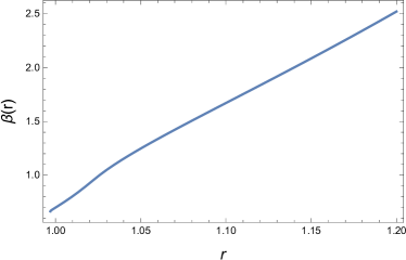
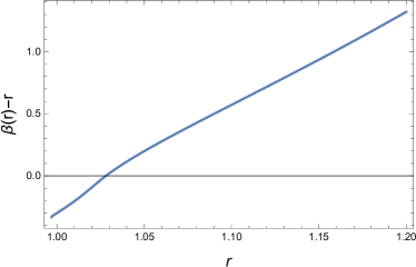
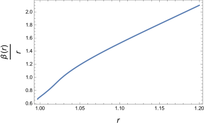
Figure 1: Plots of $\beta(r)$, $\beta(r)-r$ and $\frac{\beta(r)}{r}$ versus $r$ for the first model.

The first model is considered as [16]

$$F(T,T_{G})=-T+\gamma_{1}(T^{2}+\gamma_{2}T_{G})+\gamma_{3}(T^{2}+\gamma_{4}T_{G})^{2},$$ (13)

where $\gamma_{1}$, $\gamma_{2}$, $\gamma_{3}$ and $\gamma_{4}$ are arbitrary constants. Here, we take $\gamma_{2}$ and $\gamma_{4}$ as dimensionless whereas $\gamma_{1}$ and $\gamma_{3}$ have dimensions of lengths. This model involves second order $T_{G}$ terms and fourth order contribution from torsion term $T$. Using Eqs.(4), (5) and (13) in (12), we achieve a complicated differential equation in terms of $\beta(r)$ that cannot be handled analytically. So, we solve it numerically by choosing the corresponding parameters as $\gamma_{1}=81$, $\gamma_{2}=-0.0091$, $\gamma_{3}=12$, $\gamma_{4}=32$. The values of the remaining parameters $\mathcal{M}=15$, $\theta=0.5$ and $\psi=1$ are taken from [29]. To plot the graph of $\beta(r)$, we take the initial values as $\beta(1)=0.7$, $\beta^{\prime}(1)=9.9$ and $\beta^{\prime\prime}(1)=5.5$. Figure 1 (left panel) represents the increasing behavior of shape function $\beta(r)$. We discuss the wormhole throat by plotting $\beta(r)-r$ in the right panel.

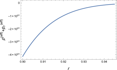
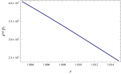
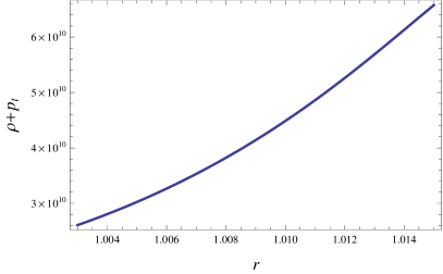
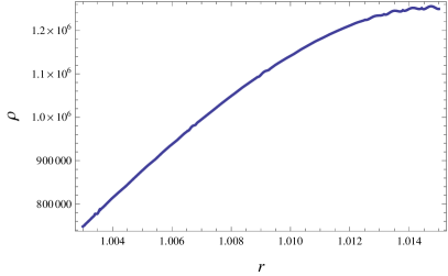
Figure 2: Plots of $\rho^{(eff)}+p_{r}^{(eff)}$, $\rho+p_{r}$, $\rho+p_{t}$ and $\rho$ versus $r$ for the first model.

As we know that throat radius is the point where $\beta(r)-r$ cuts the $r$-axis. Here, the throat radius is located at $r_{th}=1.029$ which also satisfies the condition $\beta(r)=r_{th}$ up to two digits, i.e., $\beta(1.029)=1.028$. The third graph of Figure 1 implies that the spacetime does not satisfy the asymptotically flatness condition. The upper left panel of Figure 2 represents the validity of condition (10). Thus, the violation of effective NEC confirms the presence of traversable wormhole. Also, Figure 2 shows the plots of $\rho+p_{r}$ (upper right panel), $\rho+p_{t}$ (lower left panel) and $\rho$ (lower right panel) for normal matter that exhibit positive behavior in the interval $1.003<r<1.015$. This shows that ordinary matter satisfies the NEC and physically acceptable wormhole solution is achieved for this model.

3.2 Second Model

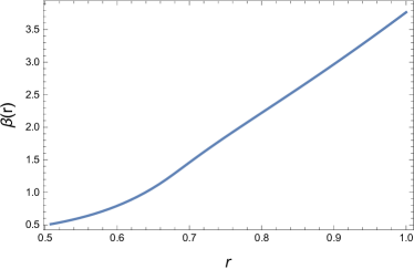
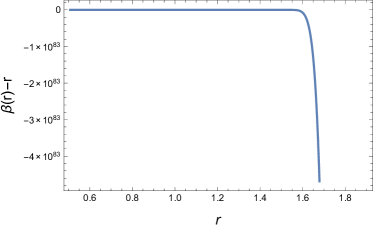
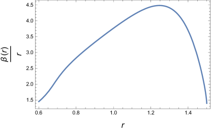
Figure 3: Plots of $\beta(r)$, $\beta(r)-r$ and $\frac{\beta(r)}{r}$ versus $r$ for the second model.

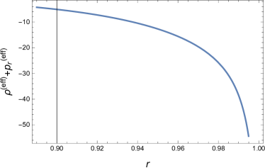
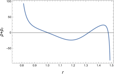
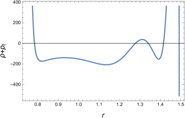
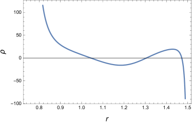
Figure 4: Plots of $\rho^{(eff)}+p_{r}^{(eff)}$, $\rho+p_{r}$, $\rho+p_{t}$ and $\rho$ versus $r$ for the second model.

We assume the second model as [11]

$$F(T,T_{G})=-T+\eta_{1}\sqrt{T^{2}+\eta_{2}T_{G}},$$ (14)

where $\eta_{1}$ and $\eta_{2}$ are the arbitrary constants. We get a differential equation by substituting Eqs.(4), (5) and (14) in (12). The numerical technique is used to calculate $\beta(r)$ from the differential equation by assuming same values of $\theta$, $\mathcal{M}$ and $\psi$ as above. The model parameters are taken as $\eta_{1}=-1.1259$ and $\eta_{2}=-0.9987$. Also, we take the following conditions: $\beta(1.5)=2.1$, $\beta^{\prime}(1.5)=-133.988$ and $\beta^{\prime\prime}(1.5)=-60000$. We discuss the properties necessary for the development of wormhole structure. The plot of shape function is shown in Figure 3 (left panel) which represents increasing behavior for all values of $r$. It can be noted that $\beta(0.5)=0.5$. In the upper right panel, we plot $\beta(r)-r$ versus $r$ to discuss the location of wormhole throat. It can be observed that small values of $r$ refer as the throat radius.

The lower graph represents the behavior of $\frac{\beta(r)}{r}$. It can be seen that as the value of $r$ increases, the curve of $\frac{\beta(r)}{r}$ approaches to $0$. Hence, the spacetime satisfies asymptotically flatness condition. The upper left panel of Figure 4 represents the negative behavior and shows the validity of condition (10). For physically acceptable wormhole solution, we check the graphical behavior of NEC and WEC for matter energy density and pressure. Figure 4 shows that $\rho+p_{r}$, $\rho+p_{t}$ and $\rho$ behave positively in the intervals $1.32\leq r\leq 1.474$, $1.28\leq r\leq 1.342$ and $1.307\leq r\leq 1.471$, respectively. The common region of these intervals are $1.28\leq r\leq 1.342$. This indicates that NEC and WEC are satisfied in a very small interval. Thus there can exist a micro or tiny physically acceptable wormhole for this model. Tiny wormhole means small radius with narrow throat.

4 Equilibrium Condition

In this section, we investigate equilibrium structure of wormhole solutions. For this purpose, we consider generalized Tolman-Oppenheimer-Volkov equation in an effective manner as

$$-p^{\prime(eff)}_{r}-(p^{(eff)}_{r}+\rho^{(eff)})\left(\frac{\alpha^{\prime}}{2}\right)+(p^{(eff)}_{t}-p^{(eff)}_{r})\left(\frac{2}{r}\right)=0,$$

with the metric $ds^{2}=diag(e^{2\alpha(r)},-e^{\nu(r)},-r^{2},-r^{2}\sin^{2}\theta)$, where $e^{\nu(r)}=\left(1\right.$-$\left.\frac{\beta(r)}{r}\right)^{-1}$. The above equation can be written as

$$-p^{\prime(eff)}_{r}-(p^{(eff)}_{r}+\rho^{(eff)})\left(\frac{M^{(eff)}e^{\frac{\alpha-\nu}{2}}}{r^{2}}\right)+(p^{(eff)}_{t}-p^{(eff)}_{r})\left(\frac{2}{r}\right)=0,$$ (15)

where the effective gravitational mass is described as $M^{(eff)}=\frac{1}{2}\left(r^{2}e^{\frac{\nu-\alpha}{2}}\right)\nu^{\prime}$. The equilibrium picture describes the stability of corresponding wormhole solutions with the help of three forces known as gravitational force $F_{gf}$, anisotropic force $F_{af}$ and hydrostatic force $F_{hf}$. The gravitational force exists because of gravitating mass, anisotropic force occurs in the presence of anisotropic system and hydrostatic force is due to hydrostatic fluid. We can rewrite Eq.(15) as

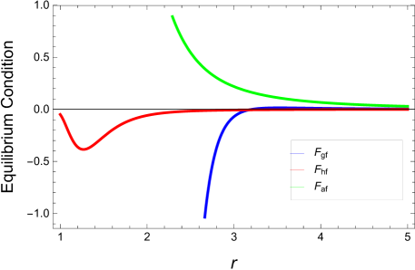
Figure 5: Plot of equilibrium condition for first model.

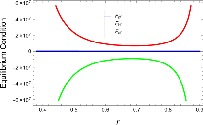
Figure 6: Plot of equilibrium condition for second model.

$$F_{hf}+F_{gf}+F_{af}=0,$$ (16)

where

$$F_{gf} = -(p_{r}^{(eff)}+\rho^{(eff)})\left(\frac{e^{\frac{\alpha-\nu}{2}}M^{(eff)}}{r^{2}}\right),F_{hf}=-p^{\prime(eff)}_{r},$$

$$F_{af} = (p_{t}^{(eff)}-p_{r}^{(eff)})\left(\frac{2}{r}\right).$$

Further, we examine the stability of wormhole solutions for first and second model through equilibrium condition. Using Eqs.(7)-(9) and (13) in (16), we obtain a difficult equation for the first model. By applying numerical technique, we plot the graphs of above defined three forces. In Figure 5, it can be easily analyzed that all the three forces cancel their effects and balance each other in the interval $4.8\leq r\leq 5$. This means that wormhole solution satisfies the equilibrium condition for the first model. Next, we take the second model and follow the same procedure by using Eq.(14). After simplification, we finally get a differential equation and solve it numerically. Figure 6 indicates that the gravitational force is zero but anisotropic and hydrostatic forces completely cancel their effects. Hence, for this model, the system is balanced which confirms the stability of the corresponding wormhole solution.

5 Concluding Remarks

In general relativity, the structure of wormhole is based on the condition that NEC is violated. This violation supports the fact that there exist a mysterious matter in the universe famous as exotic matter and distinguished by its negative energy density. The amount of this amazing matter would be minimized to obtain a physically viable wormhole. However, in modified theories, the situation may be completely different. This paper investigates noncommutative wormhole solutions with Lorentzian distribution in $F(T,T_{G})$ gravity. For this purpose, we have assumed a diagonal tetrad and a particular redshift function. We have examined these wormhole solutions graphically.

For the first model, all the properties are satisfied that are necessary for wormhole geometry regarding the shape function except asymptotic flatness. In this case, WEC and NEC for normal matter are also satisfied. Hence, this model provides realistic wormhole solution in a small interval threaded by normal matter rather than exotic matter. The violation of effective NEC confirms the traversability of the wormhole. Furthermore, the second model fulfills all properties regarding shape function and also satisfies WEC and NEC for normal matter. There exists a micro wormhole solution which is supported by normal matter. This model satisfies the traversability condition (10). We have investigated stability of both models through equilibrium condition. It is mentioned here that stability is attained for both models.

Bhar and Rahaman [28] examined in GR whether the wormhole solutions exist in different dimensional noncommutative spacetime with Lorentzian distribution. They found that wormhole solutions appear only for four and five dimensions but no solution exists for higher dimensions. It is interesting to mention here that we have also obtained wormhole solutions that satisfy all the conditions and are stable in $F(T,T_{G})$ gravity. Our results show consistency with the teleparallel equivalent of GR limits. For the first model, if we substitute $\gamma_{1}=\gamma_{3}=0$, then the behavior of shape function $\beta(r)$ and energy conditions in teleparallel theory remains the same as in this theory. For the second model, $\eta_{1}=0$ provides no result but if we consider $\eta_{2}=0$, then $\beta(r)$ as well as energy conditions represent consistent behavior.

In $F(T)$ gravity [36], the resulting noncommutative wormhole solutions are supported by normal matter by assuming diagonal tetrad. In the underlying work, we have also obtained solutions that are threaded by normal matter. Kofinas et al. [37] discussed spherically symmetric solutions in scalar-torsion gravity in which a scalar field is coupled to torsion with a derivative coupling. They obtained exact solution which represents a new wormhole-like solution having interesting physical features. We can conclude that in $F(T,T_{G})$ gravity, noncommutative geometry with Lorentzian distribution is a more favorable choice to obtain physically acceptable wormhole solutions rather than noncommutative geometry [30].

The authors have no conflict of interest for this research.

References

- [1] Kamenshchik, A.Y., Moschella, U. and Pasquier, V.: Phys. Lett. B 511(2001)265.
- [2] Li, M.: Phys. Lett. B 603(2004)1.
- [3] Cai, R.G.: Phys. Lett. B 657(2007)228.
- [4] Wei, H.: Commun. Theor. Phys. 52(2009)743.
- [5] Sheykhi, A., Jamil, M.: Gen. Relativ. Gravit. 43(2011)2661.
- [6] Linder, E.V.: Phys. Rev. D 124(2010)127301.
- [7] Ferraro, R. and Fiorini, F.: Phys. Rev. D 75(2007)084031.
- [8] Bengochea, G.R. and Ferraro, R.: Phys. Rev. D 79(2009)124019.
- [9] Linder, E.V.: Phys. Rev. D 81(2010)127301.
- [10] Kofinas, G. and Saridakis, E.N.: Phys. Rev. D 90(2014)084044.
- [11] Kofinas, G., Leon, G. and Saridakis, E.N.: Class. Quantum Grav. 31(2014)175011
- [12] Kofinas, G. and Saridakis, E.N.: Phys. Rev. D 90(2014)084045.
- [13] Chattopadhyay, S., Jawad, A., Momeni, D. and Myrzakulov, R.: Astrophys. Space Sci. 353(2014)279.
- [14] Jawad, A., Rani, S. and Chattopadhyay, S.: Astrophys. Space Sci. 360(2014)37.
- [15] Jawad, A. and Debnath, U.: Commun. Theor. Phys. 64(2015)145.
- [16] Zubair, M. and Jawad, A.: Astrophys. Space Sci. 360(2015)11.
- [17] Sharif, M. and Nazir, K.: Mod. Phys. Lett. A 31(2016)1650175; Can. J. Phys. 95(2017)297.
- [18] Agnese, A. and Camera, M.L.: Phys. Rev. D 51(1995)2011.
- [19] Anchordoqui, L.A., Bergliaffa, S.E.P. and Torres, D.F.: Phys. Rev. D 55(1997)5226.
- [20] Lobo, F.S.N. and Oliveira, M.A.: Phys. Rev. D 80(2009)104012.
- [21] Bhmer, C.G., Harko, T. and Lobo, F.S.N.: Phys. Rev. D 85(2012)044033.
- [22] Sharif, M. and Rani, S.: Gen. Relativ. Gravit. 45(2013)2389.
- [23] Sharif, M. and Ikram, A.: Int. J. Mod. Phys. D 24(2015)1550003.
- [24] Rahaman, F., Islam, S., Kuhfitting, P.K.F. and Ray, S.: Phys. Rev. D 86(2012)106010.
- [25] Abreu, E.M.C. and Sasaki, N.: arXiv:1207.7130.
- [26] Jamil, M., et al.: J. Kor. Phys. Soc. 65(2014)917.
- [27] Sharif, M. and Rani, S.: Eur. Phys. J. Plus 129(2014)237; Adv. High Energy Phys. 2014(2014)691497.
- [28] Bhar, P. and Rahaman, F.: Eur. Phys. J. Plus 74(2014)3213.
- [29] Jawad, A. and Rani, S.: Eur. Phys. J. C 75(2015)173.
- [30] Sharif, M. and Nazir, K.: Mod. Phys. Lett. A 32(2017)1750083.
- [31] Misner, C.W. and Wheeler, J.A.: Ann. Phys. 2(1957)525.
- [32] Morris, M. and Thorne, A.: Am. J. Phys. 56(1988)395.
- [33] Visser, Matt.: Lorentzian Wormholes: From Einstein to Hawking (AIP Press, New York, 1995).
- [34] Carroll, S.: Spacetime and Geometry: An Introduction to General Relativity (Addison-Wesley, 2004).
- [35] Nicolini, P., Smailagic, A. and Spalluci, E.: Phys. Lett. B 632(2006)547.
- [36] Sharif, M. and Rani, S.: Phys. Rev. D 88(2013)123501.
- [37] Kofinas, G., Papantonopoulos, E. and Saridakis, E.N.: Phys. Rev. D 91(2015)104034.