First-order Adversarial Vulnerability of Neural Networks and Input Dimension

Abstract

Over the past few years, neural networks were proven vulnerable to adversarial images: targeted but imperceptible image perturbations lead to drastically different predictions. We show that adversarial vulnerability increases with the gradients of the training objective when viewed as a function of the inputs. Surprisingly, vulnerability does not depend on network topology: for many standard network architectures, we prove that at initialization, the $\mathcal{\ell}_{1}$-norm of these gradients grows as the square root of the input dimension, leaving the networks increasingly vulnerable with growing image size. We empirically show that this dimension dependence persists after either usual or robust training, but gets attenuated with higher regularization.

1 Introduction

Following the work of Goodfellow et al. (2015), Convolutional Neural Networks (CNNs) have been found vulnerable to adversarial examples: an adversary can drive the performance of state-of-the art CNNs down to chance level with imperceptible changes to the inputs.

Based on a simple linear model, Goodfellow et al. already noted that adversarial vulnerability should depend on input dimension. Gilmer et al. (2018); Shafahi et al. (2019) later confirmed this, by showing that adversarial robustness is harder to obtain with larger input dimension. However, these results are different in nature from Goodfellow et al.’s original observation: they rely on assumptions on the dataset that amount to a form of uniformity in distribution over the input dimensions (e.g. concentric spheres, or bounded densities with full support). In the end, this analysis tends to incriminate the data: if the data can be anything, and in particular if it can spread homogeneously across many input dimensions, then robust classification gets harder.

Image datasets do not satisfy these assumptions: they do not have full support, and their probability distributions get more and more peaked with larger input dimension (pixel correlation increases). Intuitively, for image classification, higher resolution should help, not hurt. Hence data might be the wrong culprit: if we want to understand the vulnerability of our classifiers, then we should understand what is wrong with our classifiers, not with our images.

We therefore follow Goodfellow et al.’s original approach, which explains adversarial vulnerability by properties of the classifiers. Our main theoretical results start by formally extending their result for a single linear layer to almost all current deep feedforward network architectures. There is a further correction: based on the gradients of a linear layer, Goodfellow et al. predicted a linear increase of adversarial vulnerability with input dimension $d$. However, they did not take into account that a layer’s typical weights decrease like $\sqrt{d}$. Accounting for this, the dependence becomes $\sqrt{d}$ rather than $d$, which is confirmed by both our theory and experiments.

Our approach relies on evaluating the norm of gradients of the network output with respect to its inputs. At first order, adversarial vulnerability is related to gradient norms. We show that this norm is a function of input dimension only, whatever the network architecture is. The analysis is fully formal at initialization, and experiments show that the predictions remain valid throughout training with very good precision.

Obviously, this approach assumes that the classifier and loss are differentiable. So arguably it is unclear whether it can explain the vulnerability of networks with obfuscated or masked gradients. Still, Athalye et al. (2018) recently showed that masked gradients only give a false sense of security: by reconstructing gradient approximations (using differentiable nets!), the authors circumvented all state-of-the-art masked-gradient defenses. This suggests that explaining the vulnerability of differentiable nets is crucial, even for non-differentiable nets.

Although adversarial vulnerability was known to increase with gradient norms, the exact relation between the two, and the approximations made, are seldom explained, let alone tested empirically. Section 2 therefore starts with a detailed discussion of the relationship between adversarial vulnerability and gradients of the loss. Precise definitions help with sorting out all approximations used. We also revisit and formally link several old and recent defenses, such as double-backpropagation (Drucker & LeCun, 1991) and FGSM (Goodfellow et al., 2015). Section 3 proceeds with our main theoretical results on the dimension dependence of adversarial damage. Section 4 tests our predictions empirically, as well as the validity of all approximations.

Our contribution can be summarized as follows.

• We show an empirical one-to-one relationship between average gradient norms and adversarial vulnerability. This confirms that an essential part of adversarial vulnerability arises from first-order phenomena.

• We formally prove that, at initialization, the first-order vulnerability of common neural networks increases as $\sqrt{d}$ with input dimension $d$. Surprisingly, this is almost independent of the architecture. Almost all current architectures are hence, by design, vulnerable at initialization.

• We empirically show that this dimension dependence persists after both usual and robust (PGD) training, but gets dampened and eventually vanishes with higher regularization. Our experiments suggest that PGD-regularization effectively recovers dimension independent accuracy-vulnerability trade-offs.

• We observe that further training after the training loss has reached its minimum can provide improved test accuracy, but severely damages the network’s robustness. The last few accuracy points require a considerable increase of network gradients.

• We notice a striking discrepancy between the gradient norms (and therefore the vulnerability) on the training and test sets respectively. It suggests that gradient properties do not generalize well and that, outside the training set, networks may tend to revert to initialization-like gradient properties.

Overall, our results show that, without strong regularization, the gradients and vulnerability of current networks naturally tend to grow with input dimension. This suggests that current networks have too many degrees of ‘gradient-freedom’. Gradient regularization can counter-balance this to some extent, but on the long run, our networks may benefit from incorporating more data-specific knowledge. The independence of our results on the network architecture (within the range of currently common architectures) suggests that doing so would require new network modules.

Related Literature

Goodfellow et al. (2015) already noticed the dimension dependence of adversarial vulnerability. As opposed to Amsaleg et al. (2017); Gilmer et al. (2018); Shafahi et al. (2019), their (and our) explanation of the dimension dependence is data-independent. Incidentally, they also link adversarial vulnerability to loss gradients and use it to derive the FGSM adversarial augmentation defense (see Section 2). Ross & Doshi-Velez (2018) propose to robustify networks using the old double-backpropagation, but make no connection to FGSM and adversarial augmentation (see our Prop.3). Lyu et al. (2015) discuss and use the connection between gradient-penalties and adversarial augmentation, but surprisingly never empirically compare both, which we do in Section 4.1. This experiment is crucial to confirm the validity of the first-order approximation made in (2) to link adversarial damage and loss-gradients. Hein & Andriushchenko (2017) derived yet another gradient-based penalty –the cross-Lipschitz-penalty– by considering and proving formal guarantees on adversarial vulnerability (see App.D). Penalizing network-gradients is also at the heart of contractive auto-encoders as proposed by Rifai et al. (2011), where it is used to regularize the encoder-features. A gradient regularization of the loss of generative models also appears in Proposition 6 of Ollivier (2014), where it stems from a code-length bound on the data (minimum description length). For further references on adversarial attacks and defenses, see e.g. Yuan et al. (2017).

2 From Adversarial Examples to Large Gradients

Suppose that a given classifier $\varphi$ classifies an image $\bm{x}$ as being in category $\varphi(\bm{x})$. An adversarial image is a small modification of $\bm{x}$, barely noticeable to the human eye, that suffices to fool the classifier into predicting a class different from $\varphi(\bm{x})$. It is a small perturbation of the inputs, that creates a large variation of outputs. Adversarial examples thus seem inherently related to large gradients of the network. A connection that we will now clarify. Note that visible adversarial examples sometimes appear in the literature, but we deliberately focus on imperceptible ones.

Adversarial vulnerability and adversarial damage.

In practice, an adversarial image is constructed by adding a perturbation $\bm{\delta}$ to the original image $\bm{x}$ such that $\left\|\bm{\delta}\right\|\leq\epsilon$ for some (small) number $\epsilon$ and a given norm $\left\|\cdot\right\|$ over the input space. We call the perturbed input $\bm{x}+\bm{\delta}$ an $\epsilon$-sized $\left\|\cdot\right\|$-attack and say that the attack was successful when $\varphi(\bm{x}+\bm{\delta})\neq\varphi(\bm{x})$. This motivates

Definition 1.

Given a distribution $P$ over the input-space, we call adversarial vulnerability of a classifier $\varphi$ to an $\epsilon$-sized $\left\|\cdot\right\|$-attack the probability that there exists a perturbation $\bm{\delta}$ of $\bm{x}$ such that

$$\left\|\bm{\delta}\right\|\leq\epsilon\quad\text{and}\quad\varphi(\bm{x})\neq\varphi(\bm{x}+\bm{\delta})\,.$$ (1)

We call the average increase-after-attack $\mathop{\mathbb{E}_{\bm{x}\sim P}}\left[\Delta\mathcal{L}\right]$ of a loss $\mathcal{L}$ the adversarial ($\mathcal{L}$-) damage (of the classifier $\varphi$ to an $\epsilon$-sized $\left\|\cdot\right\|$-attack).

When $\mathcal{L}$ is the 0-1-loss $\mathcal{L}_{0/1}$, adversarial damage is the accuracy-drop after attack. The 0-1-loss damage is always smaller than adversarial vulnerability, because vulnerability counts all class-changes of $\varphi(\bm{x})$, whereas some of them may be neutral to adversarial damage (e.g. a change between two wrong classes). The $\mathcal{L}_{0/1}$-adversarial damage thus lower bounds adversarial vulnerability. Both are even equal when the classifier is perfect (before attack), because then every change of label introduces an error. It is hence tempting to evaluate adversarial vulnerability with $\mathcal{L}_{0/1}$-adversarial damage.

From $\Delta\mathcal{L}_{0/1}$ to $\Delta\mathcal{L}$ and to $\bm{\partial_{\scriptscriptstyle x}}\mathcal{L}$.

In practice however, we do not train our classifiers with the non-differentiable 0-1-loss but use a smoother surrogate loss $\mathcal{L}$, such as the cross-entropy loss. For similar reasons, we will now investigate the adversarial damage $\mathop{\mathbb{E}_{\bm{x}}}\left[\Delta\mathcal{L}(\bm{x},c)\right]$ with loss $\mathcal{L}$ rather than $\mathcal{L}_{0/1}$. Like for Goodfellow et al. (2015); Lyu et al. (2015); Sinha et al. (2018) and many others, a classifier $\varphi$ will hence be robust if, on average over $\bm{x}$, a small adversarial perturbation $\bm{\delta}$ of $\bm{x}$ creates only a small variation $\delta\mathcal{L}$ of the loss. Now, if $\left\|\bm{\delta}\right\|\leq\epsilon$, then a first order Taylor expansion in $\epsilon$ shows that

$$\delta\mathcal{L} =\max_{\bm{\delta}\,:\,\left\|\bm{\delta}\right\|\leq\epsilon}|\mathcal{L}(\bm{x}+\bm{\delta},c)-\mathcal{L}(\bm{x},c)|$$ (2)

$$\approx\max_{\bm{\delta}\,:\,\left\|\bm{\delta}\right\|\leq\epsilon}\left|\bm{\partial_{\scriptscriptstyle x}}\mathcal{L}\cdot\bm{\delta}\right|=\epsilon\,{\left|\kern-1.07639pt\left|\kern-1.07639pt\left|\bm{\partial_{\scriptscriptstyle x}}\mathcal{L}\right|\kern-1.07639pt\right|\kern-1.07639pt\right|},$$

where $\bm{\partial_{\scriptscriptstyle x}}\mathcal{L}$ denotes the gradient of $\mathcal{L}$ with respect to $\bm{x}$, and where the last equality stems from the definition of the dual norm ${\left|\kern-1.07639pt\left|\kern-1.07639pt\left|\cdot\right|\kern-1.07639pt\right|\kern-1.07639pt\right|}$ of $\left\|\cdot\right\|$. Now two remarks. First: the dual norm only kicks in because we let the input noise $\bm{\delta}$ optimally adjust to the coordinates of $\bm{\partial_{\scriptscriptstyle x}}\mathcal{L}$ within its $\epsilon$-constraint. This is the brand mark of adversarial noise: the different coordinates add up, instead of statistically canceling each other out as they would with random noise. For example, if we impose that $\left\|\bm{\delta}\right\|_{2}\leq\epsilon$, then $\bm{\delta}$ will strictly align with $\bm{\partial_{\scriptscriptstyle x}}\mathcal{L}$. If instead $\left\|\bm{\delta}\right\|_{\infty}\leq\epsilon$, then $\bm{\delta}$ will align with the sign of the coordinates of $\bm{\partial_{\scriptscriptstyle x}}\mathcal{L}$. Second remark: while the Taylor expansion in (2) becomes exact for infinitesimal perturbations, for finite ones it may actually be dominated by higher-order terms. Our experiments (Figures 4 & 1) however strongly suggest that in practice the first order term dominates the others. Now, remembering that the dual norm of an $\mathcal{\ell}_{p}$-norm is the corresponding $\mathcal{\ell}_{q}$-norm, and summarizing, we have proven

Lemma 2.

At first order approximation in $\epsilon$, an $\epsilon$-sized adversarial attack generated with norm $\left\|\cdot\right\|$ increases the loss $\mathcal{L}$ at point $\bm{x}$ by $\epsilon\,{\left|\kern-1.07639pt\left|\kern-1.07639pt\left|\bm{\partial_{\scriptscriptstyle x}}\mathcal{L}\right|\kern-1.07639pt\right|\kern-1.07639pt\right|}$, where ${\left|\kern-1.07639pt\left|\kern-1.07639pt\left|\cdot\right|\kern-1.07639pt\right|\kern-1.07639pt\right|}$ is the dual norm of $\left\|\cdot\right\|$. In particular, an $\epsilon$-sized $\mathcal{\ell}_{p}$-attack increases the loss by $\epsilon\left\|\bm{\partial_{\scriptscriptstyle x}}\mathcal{L}\right\|_{q}$ where $1\leq p\leq\infty$ and $\frac{1}{p}+\frac{1}{q}=1$.

Although the lemma is valid at first order only, it proves that at least this kind of first-order vulnerability is present. Moreover, we will see that the first-order predictions closely match the experiments, and that simple gradient regularization helps protecting even against iterative (non-first-order) attack methods (Figure 4).

Calibrating the threshold $\epsilon$ to the attack-norm $\left\|\cdot\right\|$.

Lemma 2 shows that adversarial vulnerability depends on three main factors: (i) $\left\|\cdot\right\|$, the norm chosen for the attack (ii) $\epsilon$, the size of the attack, and (iii) $\mathop{\mathbb{E}_{\bm{x}}}\!{\left|\kern-1.07639pt\left|\kern-1.07639pt\left|\bm{\partial_{\scriptscriptstyle x}}\mathcal{L}\right|\kern-1.07639pt\right|\kern-1.07639pt\right|}$, the expected dual norm of $\bm{\partial_{\scriptscriptstyle x}}\mathcal{L}$. We could see Point (i) as a measure of our sensibility to image perturbations, (ii) as our sensibility threshold, and (iii) as the classifier’s expected marginal sensibility to a unit perturbation. $\mathop{\mathbb{E}_{\bm{x}}}\!{\left|\kern-1.07639pt\left|\kern-1.07639pt\left|\bm{\partial_{\scriptscriptstyle x}}\mathcal{L}\right|\kern-1.07639pt\right|\kern-1.07639pt\right|}$ hence intuitively captures the discrepancy between our perception (as modeled by $\left\|\cdot\right\|$) and the classifier’s perception for an input-perturbation of small size $\epsilon$. Of course, this viewpoint supposes that we actually found a norm $\left\|\cdot\right\|$ (or more generally a metric) that faithfully reflects human perception – a project in its own right, far beyond the scope of this paper. However, it is clear that the threshold $\epsilon$ that we choose should depend on the norm $\left\|\cdot\right\|$ and hence on the input-dimension $d$. In particular, for a given pixel-wise order of magnitude of the perturbations $\bm{\delta}$, the $\mathcal{\ell}_{p}$-norm of the perturbation will scale like $d^{1/p}$. This suggests to write the threshold $\epsilon_{p}$ used with $\ell_{p}$-attacks as:

$$\epsilon_{p}=\epsilon_{\infty}\,d^{1/p}\,,$$ (3)

where $\epsilon_{\infty}$ denotes a dimension independent constant. In Appendix C we show that this scaling also preserves the average signal-to-noise ratio $\left\|\bm{x}\right\|_{2}/\left\|\bm{\delta}\right\|_{2}$, both across norms and dimensions, so that $\epsilon_{p}$ could correspond to a constant human perception-threshold. With this in mind, the impatient reader may already jump to Section 3, which contains our main contributions: the estimation of $\mathop{\mathbb{E}_{x}}\!\left\|\bm{\partial_{\scriptscriptstyle x}}\mathcal{L}\right\|_{q}$ for standard feedforward nets. Meanwhile, the rest of this section shortly discusses two straightforward defenses that we will use later and that further illustrate the role of gradients.

A new old regularizer.

Lemma 2 shows that the loss of the network after an $\frac{\epsilon}{2}$-sized $\left\|\cdot\right\|$-attack is

$$\mathcal{L}_{\epsilon,{\left|\kern-0.75346pt\left|\kern-0.75346pt\left|\cdot\right|\kern-0.75346pt\right|\kern-0.75346pt\right|}}(\bm{x},c):=\mathcal{L}(\bm{x},c)+\frac{\epsilon}{2}\,{\left|\kern-1.07639pt\left|\kern-1.07639pt\left|\bm{\partial_{\scriptscriptstyle x}}\mathcal{L}\right|\kern-1.07639pt\right|\kern-1.07639pt\right|}\,.$$ (4)

It is thus natural to take this loss-after-attack as a new training objective. Here we introduced a factor $2$ for reasons that will become clear in a moment. Incidentally, for $\left\|\cdot\right\|=\left\|\cdot\right\|_{2}$, this new loss reduces to an old regularization-scheme proposed by Drucker & LeCun (1991) called double-backpropagation. At the time, the authors argued that slightly decreasing a function’s or a classifier’s sensitivity to input perturbations should improve generalization. In a sense, this is exactly our motivation when defending against adversarial examples. It is thus not surprising to end up with the same regularization term. Note that our reasoning only shows that training with one specific norm ${\left|\kern-1.07639pt\left|\kern-1.07639pt\left|\cdot\right|\kern-1.07639pt\right|\kern-1.07639pt\right|}$ in (4) helps to protect against adversarial examples generated from $\left\|\cdot\right\|$. A priori, we do not know what will happen for attacks generated with other norms; but our experiments suggest that training with one norm also protects against other attacks (see Figure 1 and Section 4.1).

Link to adversarially augmented training.

In (1), $\epsilon$ designates an attack-size threshold, while in (4), it is a regularization-strength. Rather than a notation conflict, this reflects an intrinsic duality between two complementary interpretations of $\epsilon$, which we now investigate further. Suppose that, instead of using the loss-after-attack, we augment our training set with $\epsilon$-sized $\left\|\cdot\right\|$-attacks $\bm{x}+\bm{\delta}$, where for each training point $\bm{x}$, the perturbation $\bm{\delta}$ is generated on the fly to locally maximize the loss-increase. Then we are effectively training with

$$\tilde{\mathcal{L}}_{\epsilon,\left\|\cdot\right\|}(\bm{x},c):=\frac{1}{2}(\mathcal{L}(\bm{x},c)+\mathcal{L}(\bm{x}+\epsilon\,\bm{\delta},c))\,,$$ (5)

where by construction $\bm{\delta}$ satisfies (2). We will refer to this technique as adversarially augmented training. It was first introduced by Goodfellow et al. (2015) with $\left\|\cdot\right\|=\left\|\cdot\right\|_{\infty}$ under the name of FGSM-augmented training. Using the first order Taylor expansion in $\epsilon$ of (2), this ‘old-plus-post-attack’ loss of (5) simply reduces to our loss-after-attack, which proves

Proposition 3.

Up to first-order approximations in $\epsilon$, $\tilde{\mathcal{L}}_{\epsilon,\left\|\cdot\right\|}=\mathcal{L}_{\epsilon,{\left|\kern-0.75346pt\left|\kern-0.75346pt\left|\cdot\right|\kern-0.75346pt\right|\kern-0.75346pt\right|}}\,.$ Said differently, for small enough $\epsilon$, adversarially augmented training with $\epsilon$-sized $\left\|\cdot\right\|$-attacks amounts to penalizing the dual norm ${\left|\kern-1.07639pt\left|\kern-1.07639pt\left|\cdot\right|\kern-1.07639pt\right|\kern-1.07639pt\right|}$ of $\bm{\partial_{\scriptscriptstyle x}}\mathcal{L}$ with weight $\epsilon/2$. In particular, double-backpropagation corresponds to training with $\ell_{2}$-attacks, while FGSM-augmented training corresponds to an $\ell_{1}$-penalty on $\bm{\partial_{\scriptscriptstyle x}}\mathcal{L}$.

This correspondence between training with perturbations and using a regularizer can be compared to Tikhonov regularization: Tikhonov regularization amounts to training with random noise Bishop (1995), while training with adversarial noise amounts to penalizing $\bm{\partial_{\scriptscriptstyle x}}\mathcal{L}$. Section 4.1 verifies the correspondence between adversarial augmentation and gradient regularization empirically, which also strongly suggests the empirical validity of the first-order Taylor expansion in (2).

3 Estimating $\left\|\bm{\partial_{\scriptscriptstyle x}}\mathcal{L}\right\|_{q}$ to Evaluate Adversarial Vulnerability

In this section, we evaluate the size of $\left\|\bm{\partial_{\scriptscriptstyle x}}\mathcal{L}\right\|_{q}$ for a very wide class of standard network architectures. We show that, inside this class, the gradient-norms are independent of the network topology and increase with input dimension. We start with an intuitive explanation of these insights (Sec 3.1) before moving to our formal statements (Sec 3.2).

3.1 Core Idea: One Neuron with Many Inputs

This section is for intuition only: no assumption made here is used later. We start by showing how changing $q$ affects the size of $\left\|\bm{\partial_{\scriptscriptstyle x}}\mathcal{L}\right\|_{q}$. Suppose for a moment that the coordinates of $\bm{\partial_{\scriptscriptstyle x}}\mathcal{L}$ have typical magnitude $|\bm{\partial_{\scriptscriptstyle x}}\mathcal{L}|$. Then $\left\|\bm{\partial_{\scriptscriptstyle x}}\mathcal{L}\right\|_{q}$ scales like $d^{1/q}|\bm{\partial_{\scriptscriptstyle x}}\mathcal{L}|$. Consequently

$$\epsilon_{p}\left\|\bm{\partial_{\scriptscriptstyle x}}\mathcal{L}\right\|_{q}\ \propto\ \epsilon_{p}\,d^{1/q}\,|\bm{\partial_{\scriptscriptstyle x}}\mathcal{L}|\ \propto\ d\,|\bm{\partial_{\scriptscriptstyle x}}\mathcal{L}|\,.$$ (6)

This equation carries two important messages. First, we see how $\left\|\bm{\partial_{\scriptscriptstyle x}}\mathcal{L}\right\|_{q}$ depends on $d$ and $q$. The dependence seems highest for $q=1$. But once we account for the varying perceptibility threshold $\epsilon_{p}\propto d^{1/p}$, we see that adversarial vulnerability scales like $d\cdot|\bm{\partial_{\scriptscriptstyle x}}\mathcal{L}|$, whatever $\mathcal{\ell}_{p}$-norm we use. Second, (6) shows that to be robust against any type of $\mathcal{\ell}_{p}$-attack at any input-dimension $d$, the average absolute value of the coefficients of $\bm{\partial_{\scriptscriptstyle x}}\mathcal{L}$ must grow slower than $1/d$. Now, here is the catch, which brings us to our core insight.

In order to preserve the activation variance of the neurons from layer to layer, the neural weights are usually initialized with a variance that is inversely proportional to the number of inputs per neuron. Imagine for a moment that the network consisted only of one output neuron $o$ linearly connected to all input pixels. For the purpose of this example, we assimilate $o$ and $\mathcal{L}$. Because we initialize the weights with a variance of $1/d$, their average absolute value $|\bm{\partial}_{x}o|\equiv|\bm{\partial_{\scriptscriptstyle x}}\mathcal{L}|$ grows like $1/\sqrt{d}$, rather than the required $1/d$. By (6), the adversarial vulnerability $\epsilon\left\|\bm{\partial}_{x}o\right\|_{q}\equiv\epsilon\left\|\bm{\partial_{\scriptscriptstyle x}}\mathcal{L}\right\|_{q}$ therefore increases like ${d/\sqrt{d}=\sqrt{d}}$.

This toy example shows that the standard initialization scheme, which preserves the variance from layer to layer, causes the average coordinate-size $|\bm{\partial_{\scriptscriptstyle x}}\mathcal{L}|$ to grow like $1/\sqrt{d}$ instead of $1/d$. When an $\mathcal{\ell}_{\infty}$-attack tweaks its $\epsilon$-sized input-perturbations to align with the coordinate-signs of $\bm{\partial_{\scriptscriptstyle x}}\mathcal{L}$, all coordinates of $\bm{\partial_{\scriptscriptstyle x}}\mathcal{L}$ add up in absolute value, resulting in an output-perturbation that scales like $\epsilon\sqrt{d}$ and leaves the network increasingly vulnerable with growing input-dimension.

3.2 Formal Statements for Deep Networks

Our next theorems formalize and generalize the previous toy example to a very wide class of feedforward nets with ReLU activation functions. For illustration purposes, we start with fully connected nets before proceeding with the broader class, which includes any succession of (possibly strided) convolutional layers. In essence, the proofs iterate our insight on one layer over a sequence of layers. They all rely on the following set ($\mathcal{H}$) ​ of hypotheses:

1. Non-input neurons are followed by a ReLU killing half of its inputs, independently of the weights.

2. Neurons are partitioned into layers, meaning groups that each path traverses at most once.

3. All weights have $0$ expectation and variance $2/(\text{in-degree})$ (‘He-initialization’).

4. The weights from different layers are independent.

5. Two distinct weights $w,w^{\prime}$ from a same node satisfy $\mathop{\mathbb{E}}\left[w\,w^{\prime}\right]=0$.

If we follow common practice and initialize our nets as proposed by He et al. (2015), then H3-H5 are satisfied at initialization by design, while H1 is usually a very good approximation (Balduzzi et al., 2017). Note that such i.i.d. weight assumptions have been widely used to analyze neural nets and are at the heart of very influential and successful prior work (e.g., equivalence between neural nets and Gaussian processes as pioneered by Neal 1996). Nevertheless, they do not hold after training. That is why all our statements in this section are to be understood as orders of magnitudes that are very well satisfied at initialization both in theory and practice, and that we will confirm experimentally for trained networks in Section 4. Said differently, while our theorems rely on the statistics of neural nets at initialization, our experiments confirm their conclusions after training.

Theorem 4 (Vulnerability of Fully Connected Nets).

Consider a succession of fully connected layers with ReLU activations which takes inputs $\bm{x}$ of dimension $d$, satisfies assumptions ($\mathcal{H}$), and outputs logits $f_{k}(\bm{x})$ that get fed to a final cross-entropy-loss layer $\mathcal{L}$. Then the coordinates of $\bm{\partial_{\scriptscriptstyle{x}}}f_{\scriptscriptstyle k}$ grow like $1/\sqrt{d}$, and

$$\left\|\bm{\partial_{\scriptscriptstyle x}}\mathcal{L}\right\|_{q}\propto d^{\frac{1}{q}-\frac{1}{2}}\quad\mathrm{and}\quad\epsilon_{p}\left\|\bm{\partial_{\scriptscriptstyle x}}\mathcal{L}\right\|_{q}\propto\sqrt{d}\,.$$ (7)

These networks are thus increasingly vulnerable to $\mathcal{\ell}_{p}$-attacks with growing input-dimension.

Theorem 4 is a special case of the next theorem, which will show that the previous conclusions are essentially independent of the network-topology. We will use the following symmetry assumption on the neural connections. For a given path ${\bm{p}}$, let the path-degree $d_{\bm{p}}$ be the multiset of encountered in-degrees along path ${\bm{p}}$. For a fully connected network, this is the unordered sequence of layer-sizes preceding the last path-node, including the input-layer. Now consider the multiset $\{d_{\bm{p}}\}_{{\bm{p}}\in\mathcal{P}(x,o)}$ of all path-degrees when ${\bm{p}}$ varies among all paths from input $x$ to output $o$. The symmetry assumption (relatively to $o$) is

1. All input nodes $x$ have the same multiset $\{d_{\bm{p}}\}_{{\bm{p}}\in\mathcal{P}(x,o)}$ of path-degrees from $x$ to $o$.

Intuitively, this means that the statistics of degrees encountered along paths to the output are the same for all input nodes. This symmetry assumption is exactly satisfied by fully connected nets, almost satisfied by CNNs (up to boundary effects, which can be alleviated via periodic or mirror padding) and exactly satisfied by strided layers, if the layer-size is a multiple of the stride.

Theorem 5 (Vulnerability of Feedforward Nets).

Consider any feedforward network with linear connections and ReLU activation functions. Assume the net satisfies assumptions ($\mathcal{H}$) and outputs logits $f_{k}(\bm{x})$ that get fed to the cross-entropy-loss $\mathcal{L}$. Then $\left\|\bm{\partial_{\bm{x}}}f_{k}\right\|_{2}$ is independent of the input dimension $d$ and $\epsilon_{2}\left\|\bm{\partial_{\scriptscriptstyle x}}\mathcal{L}\right\|_{2}\propto\sqrt{d}$. Moreover, if the net satisfies the symmetry assumption ($\mathcal{S}$), then $|\partial_{\scriptscriptstyle{x}}f_{\scriptscriptstyle k}|\propto 1/\sqrt{d}$ and (7) still holds: $\left\|\bm{\partial_{\scriptscriptstyle x}}\mathcal{L}\right\|_{q}\propto d^{\frac{1}{q}-\frac{1}{2}}$ and $\epsilon_{p}\left\|\bm{\partial_{\scriptscriptstyle x}}\mathcal{L}\right\|_{q}\propto\sqrt{d}$.

Theorems 4 and 5 are proven in Appendix A. The main proof idea is that in the gradient norm computation, the He-initialization exactly compensates the combinatorics of the number of paths in the network, so that this norm becomes independent of the network topology. In particular, we get

Corollary 6 (Vulnerability of CNNs).

In any succession of convolution and dense layers, strided or not, with ReLU activations, that satisfies assumptions ($\mathcal{H}$) and outputs logits that get fed to the cross-entropy-loss $\mathcal{L}$, the gradient of the logit-coordinates scale like $1/\sqrt{d}$ and (7) is satisfied. It is hence increasingly vulnerable with growing input-resolution to attacks generated with any $\mathcal{\ell}_{p}$-norm.

Remarks.

• Appendix B shows that the network gradients are dampened when replacing strided layers by average poolings, essentially because average-pooling weights do not follow the He-init assumption H3.

• Although the principles of our analysis naturally extend to residual nets, they are not yet covered by our theorems (residual connections do not satisfy H3).

• Current weight initializations (He-, Glorot-, Xavier-) are chosen to preserve the variance from layer to layer, which constrains their scaling to $\nicefrac{{1}}{{\sqrt{\text{in-degree}}}}$. This scaling, we show, is incompatible with small gradients. But decreasing gradients simply by reducing the initial weights would kill the output signal and make training impossible for deep nets (He et al., 2015, Sec 2.2). Also note that rescaling all weights by a constant does not change the classification decisions, but it affects cross-entropy and therefore adversarial damage.

4 Empirical Results

Figure 1: Average norm $\mathop{\mathbb{E}_{\bm{x}}}\!\left\|\bm{\partial_{\scriptscriptstyle x}}\mathcal{L}\right\|$ of the loss-gradients, adversarial vulnerability and accuracy (before attack) of various networks trained with different adversarial regularization methods and regularization strengths $\epsilon$. Each point represents a trained network, and each curve a training-method. Upper row: A priori, the regularization-strengths $\epsilon$ have different meanings for each method. The near superposition of all upper-row curves illustrates $(i)$ the duality between adversarial augmentation and gradient regularization (Prop.3) and $(ii)$ confirms the rescaling of $\epsilon$ proposed in (3) and $(iii)$ supports the validity of the first-order Taylor expansion (2). $(d)$: near functional relation between adversarial vulnerability and average loss-gradient norms. $(e)$: the near-perfect linear relation between the $\mathop{\mathbb{E}}\!\left\|\bm{\partial_{\scriptscriptstyle x}}\mathcal{L}\right\|_{1}$ and $\mathop{\mathbb{E}}\!\left\|\bm{\partial_{\scriptscriptstyle x}}\mathcal{L}\right\|_{2}$ suggests that protecting against a given attack-norm also protects against others. $(f)$: Merging 1b and 1c shows that all adversarial augmentation and gradient regularization methods achieve similar accuracy-vulnerability trade-offs.

Section 4.1 empirically verifies the validity of the first-order Taylor approximation made in (2) and the correspondence between gradient regularization and adversarial augmentation (Fig.1). Section 4.2 analyzes the dimension dependence of the average gradient-norms and adversarial vulnerability after usual and robust training. Section 4.1 uses an attack-threshold $\epsilon_{\infty}=0.5\%$ of the pixel-range (invisible to humans), with PGD-attacks from the Foolbox-package (Rauber et al., 2017). Section 4.2 uses self-coded PGD-attacks with random start with $\epsilon_{\infty}=0.08\%$. As a safety-check, other attacks were tested as well (see App.4.1 & Fig.4), but results remained essentially unchanged. Note that the $\epsilon_{\infty}$-thresholds should not be confused with the regularization-strengths $\epsilon$ appearing in (4) and (5), which will be varied. The datasets were normalized ($\sigma\approx.2$). All regularization-values $\epsilon$ are reported in these normalized units (i.e. multiply by $.2$ to compare with 0-1 pixel values). Code available at https://github.com/facebookresearch/AdversarialAndDimensionality.

4.1 First-Order Approximation, Gradient Penalty, Adversarial Augmentation

We train several CNNs with same architecture to classify CIFAR-10 images (Krizhevsky, 2009). For each net, we use a specific training method with a specific regularization value $\epsilon$. The training methods used were $\ell_{1}$- and $\ell_{2}$-penalization of $\bm{\partial_{\scriptscriptstyle x}}\mathcal{L}$ (Eq. 4), adversarial augmentation with $\ell_{\infty}$- and $\ell_{2}$- attacks (Eq. 5), projected gradient descent (PGD) with randomized starts (7 steps per attack with step-size $=.2\,\epsilon_{\infty}$; see Madry et al. 2018) and the cross-Lipschitz regularizer (Eq. 18 in Appendix D). For this experiment, all networks have 6 ‘strided convolution $\rightarrow$ batchnorm $\rightarrow$ ReLU’ layers with strides [1, 2, 2, 2, 2, 2] respectively and 64 output-channels each, followed by a final fully-connected linear layer. Results are summarized in Figure 1. Each curve represents one training method. Note that our goal here is not to advocate one defense over another, but rather to check the validity of the Taylor expansion, and empirically verify that first order terms (i.e., gradients) suffice to explain much of the observed adversarial vulnerability.

Confirming first order expansion and large first-order vulnerability. The following observations support the validity of the first order Taylor expansion in (2) and suggest that it is a crucial component of adversarial vulnerability: (i) the efficiency of the first-order defense against iterative (non-first-order) attacks (Fig.1&4a); (ii) the striking similarity between the PGD curves (adversarial augmentation with iterative attacks) and the other adversarial training training curves (one-step attacks/defenses); (iii) the functional-like dependence between any approximation of adversarial vulnerability and $\mathop{\mathbb{E}_{\bm{x}}}\!\left\|\bm{\partial_{\scriptscriptstyle x}}\mathcal{L}\right\|_{1}$ (Fig.4b), and its independence on the training method (Fig.1d). (iv) the excellent correspondence between the gradient regularization and adversarial augmentation curves (see next paragraph). Said differently, adversarial examples seem indeed to be primarily caused by large gradients of the classifier as captured via the induced loss.

Gradient regularization matches adversarial augmentation (Prop.3). The upper row of Figure 1 plots $\mathop{\mathbb{E}_{\bm{x}}}\!\left\|\bm{\partial_{\scriptscriptstyle x}}\mathcal{L}_{1}\right\|$, adversarial vulnerability and accuracy as a function of $\epsilon\,d^{1/p}$. The excellent match between the adversarial augmentation curve with $p=\infty$ ($p=2$) and its gradient regularization dual counterpart with $q=1$ (resp. $q=2$) illustrates the duality between $\epsilon$ as a threshold for adversarially augmented training and as a regularization constant in the regularized loss (Proposition 3). It also supports the validity of the first-order Taylor expansion in (2).

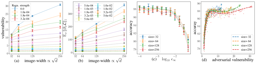
Figure 2: Input-dimension dependence of adversarial vulnerability, gradient norms and accuracy measured on up-sampled CIFAR-10 images. (b) Similar to our theorems’ prediction at initialization, average gradient norms increase like $\sqrt{d}$ yielding (a) higher vulnerability. Larger PGD-regularization during training can significantly dampen this dimension dependence with (c) almost no harm to accuracy at first (long plateau on 2c). Accuracy starts getting damaged when the dimension dependence is nearly broken ($\epsilon_{\infty}\approx.0005$). (d) Whatever the input-dimension, PGD-training achieves similar accuracy-vulnerability trade-offs. (c) & (d) suggest that PGD-training effectively recovers the original image size, 3x32x32.

Confirming correspondence of norm-dependent thresholds (Eq.3). Still on the upper row, the curves for $p=\infty,q=1$ have no reason to match those for $p=q=2$ when plotted against $\epsilon$, because the $\epsilon$-threshold is relative to a specific attack-norm. However, (3) suggested that the rescaled thresholds $\epsilon d^{1/p}$ may approximately correspond to a same ‘threshold-unit’ across $\ell_{p}$-norms and across dimension. This is well confirmed by the upper row plots: by rescaling the x-axis, the $p=q=2$ and $q=1$, $p=\infty$ curves get almost super-imposed.

Accuracy-vulnerability trade-off: confirming large first-order component of vulnerability. Merging Figures 1b and 1c by taking out $\epsilon$, Figure 1f shows that all gradient regularization and adversarial augmentation methods, including iterative ones (PGD), yield equivalent accuracy-vulnerability trade-offs. This suggest that adversarial vulnerability is largely first-order. For higher penalization values, these trade-offs appear to be much better than those given by cross Lipschitz regularization.

The regularization-norm does not matter. We were surprised to see that on Figures 1d and 1f, the $\mathcal{L}_{\epsilon,q}$ curves are almost identical for $q=1$ and $2$. This indicates that both norms can be used interchangeably in (4) (modulo proper rescaling of $\epsilon$ via (3)), and suggests that protecting against a specific attack-norm also protects against others. (6) may provide an explanation: if the coordinates of $\bm{\partial_{\scriptscriptstyle x}}\mathcal{L}$ behave like centered, uncorrelated variables with equal variance –which would follow from assumptions ($\mathcal{H}$) –, then the $\mathcal{\ell}_{1}$- and $\mathcal{\ell}_{2}$-norms of $\bm{\partial_{\scriptscriptstyle x}}\mathcal{L}$ are simply proportional. Plotting $\mathop{\mathbb{E}_{x}}\!\left\|\bm{\partial_{\scriptscriptstyle x}}\mathcal{L}(\bm{x})\right\|_{2}$ against $\mathop{\mathbb{E}_{x}}\!\left\|\bm{\partial_{\scriptscriptstyle x}}\mathcal{L}(\bm{x})\right\|_{1}$ in Figure 1e confirms this explanation. The slope is independent of the training method. (But Fig 7e shows that it is not independent of the input-dimension.) Therefore, penalizing $\left\|\bm{\partial_{\scriptscriptstyle x}}\mathcal{L}(\bm{x})\right\|_{1}$ during training will not only decrease $\mathop{\mathbb{E}_{\bm{x}}}\!\left\|\bm{\partial_{\scriptscriptstyle x}}\mathcal{L}\right\|_{1}$ (as shown in Figure 1a), but also drive down $\mathop{\mathbb{E}_{\bm{x}}}\!\left\|\bm{\partial_{\scriptscriptstyle x}}\mathcal{L}\right\|_{2}$ and vice-versa.

4.2 Vulnerability’s Dependence on Input Dimension

Theorems 4-5 and Corollary 6 predict a linear growth of the average $\mathcal{\ell}_{1}$-norm of $\bm{\partial_{\scriptscriptstyle x}}\mathcal{L}$ with the square root of the input dimension $d$, and therefore an increased adversarial vulnerability (Lemma 2). To test these predictions, we compare the vulnerability of different PGD-regularized networks when varying the input-dimension. To do so, we resize the original 3x32x32 CIFAR-10 images to 32, 64, 128 and 256 pixels per edge by copying adjacent pixels, and train one CNN for each input-size and regularization strength $\epsilon$. All nets had the same amount of parameters and very similar structure across input-resolutions (see Appendix G.1). All reported values were computed over the last 20 training epochs on the same held-out test-set.

Gradients and vulnerability increase with $\sqrt{d}$. Figures 2a &2b summarize the resulting dimension dependence of gradient-norms and adversarial vulnerability. The dashed-lines follow the medians of the 20 last epochs and the errorbars show their 10 and 90 quantiles. Similar to the predictions of our theorems at initialization, we see that, even after training, $\mathop{\mathbb{E}_{\bm{x}}}\left[\left\|\bm{\partial_{\scriptscriptstyle x}}\mathcal{L}\right\|_{1}\right]$ grows linearly with $\sqrt{d}$ which yields higher adversarial vulnerability. However, increasing the regularization decreases the slope of this dimension dependence until, eventually, the dependence breaks.

Accuracies are dimension independent. Figure 2c plots accuracy versus regularization strength, with errorbars summarizing the 20 last training epochs. The four curves correspond to the four different input dimensions. They overlap, which confirms that contrary to vulnerability, the accuracies are dimension independent; and that the $\mathcal{\ell}_{\infty}$-attack thresholds are essentially dimension independent.

PGD effectively recovers original input dimension. Figure 2d plots the accuracy-vulnerability trade-offs achieved by the previous nets over their 20 last training epochs, with a smoothing spline fitted for each input dimension (scipy’s UnivariateSpline with s=200). Higher dimensions have a longer plateau to the right, because without regularization, vulnerability increases with input dimension. The curves overlap when moving to the left, meaning that the accuracy-vulnerability trade-offs achieved by PGD are essentially independent of the actual input dimension.

PGD training outperforms down-sampling. On artificially upsampled CIFAR-10 images, PGD regularization acts as if it first reduced the images back to their original size before classifying them. Can PGD outperform this strategy when the original image is really high resolution? To test this, we create a 12-class ‘Mini-ImageNet’ dataset with approximately 80,000 images of size 3x256x256 by merging similar ImageNet classes and center-cropping/resizing as needed. We then do the same experiment as with up-sampled CIFAR-10, but using down-sampling instead of up-sampling (Appendix H, Fig. 13). While the dependence of vulnerability to the dimension stays essentially unchanged, PGD training now achieves much better accuracy-vulnerability trade-offs with the original high-dimensional images than with their down-sampled versions.

Insights from figures in Appendix G. Appendix G reproduces many additional figures on this section’s experiments. They yield additional insights which we summarize here.

Non-equivalence of loss- and accuracy-damage. Figure 8a&c show that the test-error continues to decrease all over training, while the cross-entropy increases on the test set from epoch $\approx 40$ and on. This aligns with the observations and explanations of Soudry et al. (2018). But it also shows that one must be careful when substituting their differentials, loss- and accuracy-damage. (See also Fig.9b.)

Early stopping dampens vulnerability. Fig.8 shows that adversarial damage and vulnerability closely follow the evolution of cross-entropy. Since cross-entropy overfits, early stopping effectively acts as a defense. See Fig.10.

Gradient norms do not generalize well. Figure 12 reveals a strong discrepancy between the average gradient norms on the test and the training data. This discrepancy increases over training (gradient norms decrease on the training data but increase on the test set), and with the input dimension, as $\sqrt{d}$. This dimension dependence might suggest that, outside the training points, the networks tend to recover initial gradient properties. Our observations confirm Schmidt et al.’s (2018) recent finding that PGD-regularization has a hard time generalizing to the test-set. They claim that better generalization requires more data. Alternatively, we could try to rethink our network modules to adapt it to the data, e.g. by decreasing their degrees of ‘gradient-freedom’. Evaluating the gradient-sizes at initialization may help doing so.

5 Conclusion

For differentiable classifiers and losses, we showed that adversarial vulnerability increases with the gradients $\bm{\partial_{\scriptscriptstyle x}}\mathcal{L}$ of the loss. All approximations made are fully specified, and validated by the near-perfect functional relationship between gradient norms and vulnerability (Fig.1d). We evaluated the size of $\left\|\bm{\partial_{\scriptscriptstyle x}}\mathcal{L}\right\|_{q}$ and showed that, at initialization, many current feedforward nets (convolutional or fully connected) are increasingly vulnerable to $\mathcal{\ell}_{p}$-attacks with growing input dimension (image size), independently of their architecture. Our experiments confirm this dimension dependence after usual training, but PGD-regularization dampens it and can effectively counter-balance the effect of artificial input dimension augmentation. Nevertheless, regularizing beyond a certain point yields a rapid decrease in accuracy, even though at that point many adversarial examples are still visually undetectable for humans. Moreover, the gradient norms remain much higher on test than on training examples. This suggests that even with PGD robustification, there are still significant statistical differences between the network’s behavior on the training and test sets. Given the generality of our results in terms of architectures, this can perhaps be alleviated only via tailored architectural constraints on the gradients of the network. Based on these theoretical insights, we hypothesize that tweaks on the architecture may not be sufficient, and coping with the phenomenon of adversarial examples will require genuinely new ideas.

Acknowledgements

We thank Martín Arjovsky, Ilya Tolstikhin and Diego Fioravanti for helpful discussions.

Appendix A Proofs

A.1 Proof of Proposition 3

Proof.

Let $\epsilon\,\bm{\delta}$ be an adversarial perturbation with $\left\|\bm{\delta}\right\|=1$ that locally maximizes the loss increase at point $\bm{x}$, meaning that $\bm{\delta}=\mathrm{arg\,max}_{\left\|\bm{\delta}^{\prime}\right\|\leq 1}\bm{\partial_{\scriptscriptstyle x}}\mathcal{L}\cdot\bm{\delta}^{\prime}$. Then, by definition of the dual norm of $\bm{\partial_{\scriptscriptstyle x}}\mathcal{L}$ we have: $\bm{\partial_{\scriptscriptstyle x}}\mathcal{L}\cdot(\epsilon\bm{\delta})=\epsilon\,{\left|\kern-1.07639pt\left|\kern-1.07639pt\left|\bm{\partial_{\scriptscriptstyle x}}\mathcal{L}\right|\kern-1.07639pt\right|\kern-1.07639pt\right|}$. Thus

$$\tilde{\mathcal{L}}_{\epsilon,\left\|\cdot\right\|}(\bm{x},c) =\frac{1}{2}(\mathcal{L}(\bm{x},c)+\mathcal{L}(\bm{x}+\epsilon\,\bm{\delta},c))$$

$$=\frac{1}{2}(2\mathcal{L}(\bm{x},c)+\epsilon\left|\bm{\partial_{\scriptscriptstyle x}}\mathcal{L}\cdot\bm{\delta}\right|+o(\left\|\bm{\delta}\right\|))$$

$$=\mathcal{L}(\bm{x},c)+\frac{\epsilon}{2}\,{\left|\kern-1.07639pt\left|\kern-1.07639pt\left|\bm{\partial_{\scriptscriptstyle x}}\mathcal{L}\right|\kern-1.07639pt\right|\kern-1.07639pt\right|}+o(\epsilon)$$

$$=\mathcal{L}_{\epsilon,{\left|\kern-0.75346pt\left|\kern-0.75346pt\left|\cdot\right|\kern-0.75346pt\right|\kern-0.75346pt\right|}}(\bm{x},c)+o(\epsilon)\,.\qed$$

A.2 Proof of Theorem 4

Proof.

Let $x$ designate a generic coordinate of $\bm{x}$. To evaluate the size of $\left\|\bm{\partial_{\scriptscriptstyle x}}\mathcal{L}\right\|_{q}$, we will evaluate the size of the coordinates $\partial_{\scriptscriptstyle{x}}\mathcal{L}$ of $\bm{\partial_{\scriptscriptstyle x}}\mathcal{L}$ by decomposing them into

$$\partial_{\scriptscriptstyle{x}}\mathcal{L}=\sum_{k=1}^{K}\frac{\partial\mathcal{L}}{\partial f_{k}}\frac{\partial f_{k}}{\partial x}=:\sum_{k=1}^{K}\partial_{\scriptscriptstyle{k}}\mathcal{L}\,\partial_{\scriptscriptstyle{x}}f_{\scriptscriptstyle k},$$

where $f_{k}(\bm{x})$ denotes the logit-probability of $\bm{x}$ belonging to class $k$. We now investigate the statistical properties of the logit gradients $\bm{\partial_{\scriptscriptstyle{x}}}f_{\scriptscriptstyle k}$, and then see how they shape $\partial_{\scriptscriptstyle{x}}\mathcal{L}$.

Step 1: Statistical properties of $\bm{\partial_{\scriptscriptstyle{x}}}f_{\scriptscriptstyle k}$.

Let $\mathcal{P}(x,k)$ be the set of paths ${\bm{p}}$ from input neuron $x$ to output-logit $k$. Let $p-1$ and $p$ be two successive neurons on path ${\bm{p}}$, and $\tilde{\bm{p}}$ be the same path ${\bm{p}}$ but without its input neuron. Let $w_{p}$ designate the weight from $p-1$ to $p$ and $\omega_{{\bm{p}}}$ be the path-product $\omega_{\bm{p}}:=\prod_{p\in\tilde{\bm{p}}}w_{p}$. Finally, let $\sigma_{p}$ (resp. $\sigma_{\bm{p}}$) be equal to 1 if the ReLU of node $p$ (resp. if path ${\bm{p}}$) is active for input $\bm{x}$, and 0 otherwise.

As previously noticed by Balduzzi et al. (2017) using the chain rule, we see that $\partial_{\scriptscriptstyle{x}}f_{\scriptscriptstyle k}$ is the sum of all $\omega_{\bm{p}}$ whose path is active, i.e. $\partial_{\scriptscriptstyle{x}}f_{\scriptscriptstyle k}(\bm{x})=\sum_{{\bm{p}}\in\mathcal{P}(x,k)}\omega_{\bm{p}}\sigma_{\bm{p}}.$ Consequently:

$$\mathop{\mathbb{E}_{W,\sigma}}\left[\partial_{\scriptscriptstyle{x}}f_{\scriptscriptstyle k}(\bm{x})^{2}\right]=\sum_{{\bm{p}}\in\mathcal{P}(x,k)}\prod_{p\in\tilde{\bm{p}}}\mathop{\mathbb{E}_{W}}\left[w_{p}^{2}\right]\mathop{\mathbb{E}_{\sigma}}\left[\sigma_{p}^{2}\right]\\ =|\mathcal{P}(x,k)|\prod_{p\in\tilde{\bm{p}}}\frac{2}{d_{p-1}}\frac{1}{2}=\prod_{p\in\tilde{\bm{p}}}d_{p}\cdot\prod_{p\in\tilde{\bm{p}}}\frac{1}{d_{p-1}}=\frac{1}{d}\,.$$ (8)

The first equality uses H1 to decouple the expectations over weights and ReLUs, and then applies Lemma 9 of Appendix A.3, which uses H3-H5 to kill all cross-terms and take the expectation over weights inside the product. The second equality uses H3 and the fact that the resulting product is the same for all active paths. The third equality counts the number of paths from $x$ to $k$ and we conclude by noting that all terms cancel out, except $d_{p-1}$ from the input layer which is $d$. Equation 8 shows that $|\partial_{\scriptscriptstyle{x}}f_{\scriptscriptstyle k}|\propto 1/\sqrt{d}$.

Step 2: Statistical properties of $\partial_{\scriptscriptstyle{k}}\mathcal{L}$ and $\partial_{\scriptscriptstyle{x}}\mathcal{L}$.

Defining $q_{k}(\bm{x}):=\frac{e^{f_{k}(\bm{x})}}{\sum_{h=1}^{K}e^{f_{h}(\bm{x})}}$ (the probability of image $x$ belonging to class $k$ according to the network), we have, by definition of the cross-entropy loss, $\mathcal{L}(\bm{x},c):=-\log q_{c}(\bm{x})$, where $c$ is the label of the target class. Thus:

$$\partial_{\scriptscriptstyle{k}}\mathcal{L}(\bm{x})=\left\{\begin{array}[]{ll}-q_{k}(\bm{x})&\text{if }k\neq c\\ 1-q_{c}(\bm{x})&\text{otherwise},\end{array}\right.\quad\text{and}$$

$$\partial_{\scriptscriptstyle{x}}\mathcal{L}(\bm{x})=(1-q_{c})\,\partial_{\scriptscriptstyle{x}}f_{\scriptscriptstyle c}(\bm{x})+\sum_{k\neq c}q_{k}\,(-\partial_{\scriptscriptstyle{x}}f_{\scriptscriptstyle k}(\bm{x})).$$ (9)

Using again Lemma 9, we see that the $\partial_{\scriptscriptstyle{x}}f_{\scriptscriptstyle k}(\bm{x})$ are $K$ centered and uncorrelated variables. So $\partial_{\scriptscriptstyle{x}}\mathcal{L}(\bm{x})$ is approximately the sum of $K$ uncorrelated variables with zero-mean, and its total variance is given by $\big{(}(1-q_{c})^{2}+\sum_{k\neq c}q_{k}^{2}\big{)}/d$. Hence the magnitude of $\partial_{\scriptscriptstyle{x}}\mathcal{L}(\bm{x})$ is $1/\sqrt{d}$ for all $\bm{x}$, so the $\mathcal{\ell}_{q}$-norm of the full input gradient is $d^{1/q-1/2}$. (6) concludes. ∎

Remark 1.

Equation 9 can be rewritten as

$$\partial_{\scriptscriptstyle{x}}\mathcal{L}(\bm{x})=\sum_{k=1}^{K}q_{k}(\bm{x})\,\big{(}\partial_{\scriptscriptstyle{x}}f_{\scriptscriptstyle c}(\bm{x})-\partial_{\scriptscriptstyle{x}}f_{\scriptscriptstyle k}(\bm{x})\big{)}\ .$$ (10)

As the term $k=c$ disappears, the norm of the gradients $\partial_{\scriptscriptstyle{x}}\mathcal{L}(\bm{x})$ appears to be controlled by the total error probability. This suggests that, even without regularization, trying to decrease the ordinary classification error is still a valid strategy against adversarial examples. It reflects the fact that when increasing the classification margin, larger gradients of the classifier’s logits are needed to push images from one side of the classification boundary to the other. This is confirmed by Theorem 2.1 of Hein & Andriushchenko (2017). See also (17) in Appendix D.

A.3 Proof of Theorem 5

The proof of Theorem 5 is very similar to the one of Theorem 4, but we will need to first generalize the equalities appearing in (8). To do so, we identify the computational graph of a neural network to an abstract Directed Acyclic Graph (DAG) which we use to prove the needed algebraic equalities. We then concentrate on the statistical weight-interactions implied by assumption ($\mathcal{H}$), and finally throw these results together to prove the theorem. In all the proof, $o$ will designate one of the output-logits $f_{k}(\bm{x})$.

Lemma 7.

Let $\bm{x}$ be the vector of inputs to a given DAG, $o$ be any leaf-node of the DAG, $x$ a generic coordinate of $\bm{x}$. Let ${\bm{p}}$ be a path from the set of paths $\mathcal{P}(x,o)$ from $x$ to $o$, $\tilde{\bm{p}}$ the same path without node $x$, $p$ a generic node in $\tilde{\bm{p}}$, and $d_{p}$ be its input-degree. Then:

$$\sum_{x\in\bm{x}}\sum_{\tilde{\bm{p}}\in\mathcal{P}(x,o)}\prod_{p\in\tilde{\bm{p}}}\frac{1}{d_{p}}=1$$ (11)

Proof.

We will reason on a random walk starting at $o$ and going up the DAG by choosing any incoming node with equal probability. The DAG being finite, this walk will end up at an input-node $x$ with probability $1$. Each path ${\bm{p}}$ is taken with probability $\prod_{p\in\tilde{\bm{p}}}\frac{1}{d_{p}}$. And the probability to end up at an input-node is the sum of all these probabilities, i.e. $\sum_{x\in\bm{x}}\sum_{{\bm{p}}\in\mathcal{P}(x,o)}\prod_{p\in{\bm{p}}}d_{p}^{-1}$, which concludes. ∎

The sum over all inputs $x$ in (11) being 1, on average it is $1/d$ for each $x$, where $d$ is the total number of inputs (i.e. the length of $\bm{x}$). It becomes an equality under assumption ($\mathcal{S}$):

Lemma 8.

Under the symmetry assumption ($\mathcal{S}$), and with the previous notations, for any input $x\in\bm{x}$:

$$\sum_{{\bm{p}}\in\mathcal{P}(x,o)}\prod_{p\in\tilde{\bm{p}}}\frac{1}{d_{p}}=\frac{1}{d}\,.$$ (12)

Proof.

Let us denote $\mathcal{D}(x,o):=\{d_{\bm{p}}\}_{x\in\mathcal{P}(x,o)}$. Each path ${\bm{p}}$ in $\mathcal{P}(x,o)$ corresponds to exactly one element $d_{\bm{p}}$ in $\mathcal{D}(x,o)$ and vice-versa. And the elements $d_{p}$ of $d_{\bm{p}}$ completely determine the product $\prod_{p\in\tilde{\bm{p}}}d_{p}^{-1}$. By using (11) and the fact that, by ($\mathcal{S}$), the multiset $\mathcal{D}(x,o)$ is independent of $x$, we hence conclude

$$\sum_{x\in\bm{x}}\sum_{{\bm{p}}\in\mathcal{P}(x,o)}\prod_{p\in\tilde{\bm{p}}}\frac{1}{d_{p}} =\sum_{x\in\bm{x}}\sum_{d_{\bm{p}}\in\mathcal{D}(x,o)}\prod_{d_{p}\in d_{\bm{p}}}\frac{1}{d_{p}}$$

$$=d\sum_{d_{\bm{p}}\in\mathcal{D}(x,o)}\prod_{d_{p}\in d_{\bm{p}}}\frac{1}{d_{p}}=1\,.$$ ∎

Now, let us relate these considerations on graphs to gradients and use assumptions ($\mathcal{H}$). We remind that path-product $\omega_{\bm{p}}$ is the product $\prod_{p\in\tilde{\bm{p}}}w_{p}$.

Lemma 9.

Under assumptions ($\mathcal{H}$), the path-products $\omega_{{\bm{p}}},\omega_{{\bm{p}}^{\prime}}$ of two distinct paths ${\bm{p}}$ and ${\bm{p}}^{\prime}$ starting from a same input node $x$, satisfy:

$$\mathop{\mathbb{E}_{W}}\left[\omega_{\bm{p}}\,\omega_{{\bm{p}}^{\prime}}\right]=0\quad\text{and}\quad\mathop{\mathbb{E}_{W}}\left[\omega_{\bm{p}}^{2}\right]=\prod_{p\in\tilde{\bm{p}}}\mathop{\mathbb{E}_{W}}\left[w_{p}^{2}\right]\,.$$

Furthermore, if there is at least one non-average-pooling weight on path ${\bm{p}}$, then $\mathop{\mathbb{E}_{W}}\left[\omega_{{\bm{p}}}\right]=0$.

Proof.

Hypothesis H4 yields

$$\mathop{\mathbb{E}_{W}}\left[\omega_{\bm{p}}^{2}\right]=\mathop{\mathbb{E}_{W}}\left[\prod_{p\in\tilde{\bm{p}}}w_{p}^{2}\right]=\prod_{p\in\tilde{\bm{p}}}\mathop{\mathbb{E}_{W}}\left[w_{p}^{2}\right]\,.$$

Now, take two different paths ${\bm{p}}$ and ${\bm{p}}^{\prime}$ that start at a same node $x$. Starting from $x$, consider the first node after which ${\bm{p}}$ and ${\bm{p}}^{\prime}$ part and call $p$ and $p^{\prime}$ the next nodes on ${\bm{p}}$ and ${\bm{p}}^{\prime}$ respectively. Then the weights $w_{p}$ and $w_{p^{\prime}}$ are two weights of a same node. Applying H4 and H5 hence gives

$$\mathop{\mathbb{E}_{W}}\left[\omega_{\bm{p}}\,\omega_{{\bm{p}}^{\prime}}\right]=\mathop{\mathbb{E}_{W}}\left[\omega_{{\bm{p}}\backslash p}\,\omega_{{\bm{p}}^{\prime}\backslash p^{\prime}}\right]\mathop{\mathbb{E}_{W}}\left[w_{p}\,w_{p^{\prime}}\right]=0\,.$$

Finally, if ${\bm{p}}$ has at least one non-average-pooling node $p$, then successively applying H4 and H3 yields: $\mathop{\mathbb{E}_{W}}\left[\omega_{{\bm{p}}}\right]=\mathop{\mathbb{E}_{W}}\left[\omega_{{\bm{p}}\backslash p}\right]\mathop{\mathbb{E}_{W}}\left[w_{p}\right]=0$. ∎

We now have all elements to prove Theorem 5.

Proof.

(of Theorem 5) For a given neuron $p$ in $\tilde{\bm{p}}$, let $p-1$ designate the previous node in ${\bm{p}}$ of $p$. Let $\sigma_{p}$ (resp. $\sigma_{\bm{p}}$) be a variable equal to $0$ if neuron $p$ gets killed by its ReLU (resp. path ${\bm{p}}$ is inactive), and 1 otherwise. Then:

$$\partial_{x}o\ =\sum_{{\bm{p}}\in\mathcal{P}(x,o)}\prod_{p\in\tilde{\bm{p}}}\partial_{p-1}\,p\ =\sum_{{\bm{p}}\in\mathcal{P}(x,o)}\omega_{\bm{p}}\,\sigma_{\bm{p}}$$

Consequently:

$$\mathop{\mathbb{E}_{W,\sigma}}\left[(\partial_{x}o)^{2}\right] =\sum_{{\bm{p}},{\bm{p}}^{\prime}\in\mathcal{P}(x,o)}\mathop{\mathbb{E}_{W}}\left[\omega_{\bm{p}}\,\omega_{{\bm{p}}^{\prime}}\right]\mathop{\mathbb{E}_{\sigma}}\left[\sigma_{\bm{p}}\sigma_{{\bm{p}}^{\prime}}\right]$$

$$=\sum_{{\bm{p}}\in\mathcal{P}(x,o)}\prod_{p\in\tilde{\bm{p}}}\mathop{\mathbb{E}_{W}}\left[\omega_{p}^{2}\right]\mathop{\mathbb{E}_{\sigma}}\left[\sigma_{p}^{2}\right]$$ (13)

$$=\sum_{{\bm{p}}\in\mathcal{P}(x,o)}\prod_{p\in\tilde{\bm{p}}}\frac{2}{d_{p}}\,\frac{1}{2}=\frac{1}{d}\,,$$

where the first line uses the independence between the ReLU killings and the weights (H1), the second uses Lemma 9 and the last uses Lemma 8. The gradient $\bm{\partial_{\bm{x}}}o$ thus has coordinates whose squared expectations scale like $1/d$. Thus each coordinate scales like $1/\sqrt{d}$ and $\left\|\bm{\partial_{\bm{x}}}o\right\|_{q}$ like $d^{1/2-1/q}$. Conclude on $\left\|\bm{\partial_{\scriptscriptstyle x}}\mathcal{L}\right\|_{q}$ and $\epsilon_{p}\left\|\bm{\partial_{\scriptscriptstyle x}}\mathcal{L}\right\|_{q}$ by using Step 2 of the proof of Theorem 4.

Finally, note that, even without the symmetry assumption ($\mathcal{S}$), using Lemma 7 shows that

$$\mathop{\mathbb{E}_{W}}\left[\left\|\bm{\partial_{\bm{x}}}o\right\|_{2}^{2}\right] =\sum_{x\in\bm{x}}\mathop{\mathbb{E}_{W}}\left[(\partial_{x}o)^{2}\right]$$

$$=\sum_{x\in\bm{x}}\sum_{{\bm{p}}\in\mathcal{P}(x,o)}\prod_{p\in\tilde{\bm{p}}}\frac{2}{d_{p}}\,\frac{1}{2}=1\,.$$

Thus, with or without ($\mathcal{S}$), $\left\|\bm{\partial_{\bm{x}}}o\right\|_{2}$ is independent of the input-dimension $d$. ∎

A.4 Proof of Theorem 11

To prove Theorem 11, we will actually prove the following more general theorem, which generalizes Theorem 5. Theorem 11 is a straightforward corollary of it.

Theorem 10.

Consider any feedforward network with linear connections and ReLU activation functions that outputs logits $f_{k}(\bm{x})$ and satisfies assumptions ($\mathcal{H}$). Suppose that there is a fixed multiset of integers $\{a_{1},\ldots,a_{n}\}$ such that each path from input to output traverses exactly $n$ average pooling nodes with degrees $\{a_{1},\ldots,a_{n}\}$. Then:

$$\left\|\partial_{\scriptscriptstyle{x}}f_{\scriptscriptstyle k}\right\|_{2}\propto\frac{1}{\prod_{i=1}^{n}\sqrt{a_{i}}}\,.$$ (14)

Furthermore, if the net satisfies the symmetry assumption ($\mathcal{S}$), then: $|\partial_{\scriptscriptstyle{x}}f_{\scriptscriptstyle k}|\propto\frac{1}{\sqrt{d\prod_{i=1}^{n}a_{i}}}.$

Two remarks. First, in all this proof, “weight” encompasses both the standard random weights, and the constant (deterministic) weights equal to $1/(\text{in-degree})$ of the average-poolings. Second, assumption H5 implies that the average-pooling nodes have disjoint input nodes: otherwise, there would be two non-zero deterministic weights $w,w^{\prime}$ from a same neuron that would hence satisfy: $\mathop{\mathbb{E}_{W}}\left[w\,w^{\prime}\right]\neq 0$.

Proof.

As previously, let $o$ designate any fixed output-logit $f_{k}(\bm{x})$. For any path ${\bm{p}}$, let ${\bm{a}}$ be the set of average-pooling nodes of ${\bm{p}}$ and let ${\bm{q}}$ be the set of remaining nodes. Each path-product $\omega_{\bm{p}}$ satisfies: $\omega_{{\bm{p}}}=\omega_{{\bm{q}}}\omega_{{\bm{a}}}$, where $\omega_{{\bm{a}}}$ is a same fixed constant. For two distinct paths ${\bm{p}},{\bm{p}}^{\prime}$, Lemma 9 therefore yields: $\mathop{\mathbb{E}_{W}}\left[\omega_{{\bm{p}}}^{2}\right]=\omega_{{\bm{a}}}^{2}\mathop{\mathbb{E}_{W}}\left[\omega_{{\bm{q}}}^{2}\right]$ and $\mathop{\mathbb{E}_{W}}\left[\omega_{{\bm{p}}}\omega_{{\bm{p}}^{\prime}}\right]=0$. Combining this with Lemma 8 and under assumption ($\mathcal{S}$), we get similarly to (A.3):

$$\mathop{\mathbb{E}_{W,\sigma}}\left[(\partial_{x}o)^{2}\right] =\!\!\!\!\!\sum_{{\bm{p}},{\bm{p}}^{\prime}\in\mathcal{P}(x,o)}\!\!\!\!\!\omega_{{\bm{a}}}\omega_{{\bm{a}}^{\prime}}\mathop{\mathbb{E}_{W}}\left[\omega_{\bm{q}}\,\omega_{{\bm{q}}^{\prime}}\right]\mathop{\mathbb{E}_{\sigma}}\left[\sigma_{\bm{q}}\sigma_{{\bm{q}}^{\prime}}\right]$$

$$=\sum_{{\bm{p}}\in\mathcal{P}(x,o)}\prod_{i=1}^{n}\frac{1}{a_{i}^{2}}\,\prod_{q\in\tilde{\bm{q}}}\mathop{\mathbb{E}_{W}}\left[\omega_{q}^{2}\right]\mathop{\mathbb{E}_{\sigma}}\left[\sigma_{q}^{2}\right]$$

$$=\underbrace{\prod_{i=1}^{n}\frac{1}{a_{i}}}_{\begin{subarray}{c}\text{same value}\\ \text{for all }{\bm{p}}\end{subarray}}\smash{\underbrace{\sum_{{\bm{p}}\in\mathcal{P}(x,o)}\underbrace{\prod_{i=1}^{n}\frac{1}{a_{i}}\prod_{q\in\tilde{\bm{q}}}\frac{2}{d_{q}}\,\frac{1}{2}}_{\prod_{p\in\tilde{\bm{p}}}\frac{1}{d_{p}}}}_{=\frac{1}{d}\ \ \text{(Lemma~{}\ref{symdag})}}}$$ (15)

$$=\frac{1}{d}\prod_{i=1}^{n}\frac{1}{a_{i}}\,.$$

Therefore, $|\partial_{x}o|=|\partial_{\scriptscriptstyle{x}}f_{\scriptscriptstyle k}|\propto 1/\sqrt{d\prod_{i=1}^{n}a_{i}}$. Again, note that, even without assumption ($\mathcal{S}$), using (A.4) and Lemma 7 shows that

$$\mathop{\mathbb{E}_{W}}\left[\left\|\bm{\partial_{\bm{x}}}o\right\|_{2}^{2}\right] =\sum_{x\in\bm{x}}\mathop{\mathbb{E}_{W,\sigma}}\left[(\partial_{x}o)^{2}\right]$$

$$\stackrel{{\scriptstyle\eqref{varEqPool}}}{{=}}\sum_{x\in\bm{x}}\prod_{i=1}^{n}\frac{1}{a_{i}}\sum_{{\bm{p}}\in\mathcal{P}(x,o)}\prod_{i=1}^{n}\frac{1}{a_{i}}\prod_{p\in\tilde{\bm{p}}}\frac{2}{d_{p}}\,\frac{1}{2}$$

$$=\prod_{i=1}^{n}\frac{1}{a_{i}}\,\underbrace{\sum_{x\in\bm{x}}\sum_{{\bm{p}}\in\mathcal{P}(x,o)}\prod_{p\in\tilde{\bm{p}}}\frac{1}{d_{p}}}_{=1\text{ (Lemma~{}\ref{dag})}}=\prod_{i=1}^{n}\frac{1}{a_{i}}\,,$$

which proves (14). ∎

Appendix B Effects of Strided and Average-Pooling Layers on Adversarial Vulnerability

It is common practice in CNNs to use average-pooling layers or strided convolutions to progressively decrease the number of pixels per channel. Corollary 6 shows that using strided convolutions does not protect against adversarial examples. However, what if we replace strided convolutions by convolutions with stride 1 plus an average-pooling layer? Theorem 5 considers only randomly initialized weights with typical size $1/\sqrt{\text{in-degree}}$. Average-poolings however introduce deterministic weights of size $1/(\text{in-degree})$. These are smaller and may therefore dampen the input-to-output gradients and protect against adversarial examples. We confirm this in our next theorem, which uses a slightly modified version ($\mathcal{H}^{\prime}$) of ($\mathcal{H}$) to allow average pooling layers. ($\mathcal{H}^{\prime}$) is ($\mathcal{H}$), but where the He-init H3 applies to all weights except the (deterministic) average pooling weights, and where H1 places a ReLU on every non-input and non-average-pooling neuron.

Theorem 11 (Effect of Average-Poolings).

Consider a succession of convolution layers, dense layers and $n$ average-pooling layers, in any order, that satisfies ($\mathcal{H}^{\prime}$) and outputs logits $f_{k}(\bm{x})$. Assume the $n$ average pooling layers have a stride equal to their mask size and perform averages over $a_{1}$, …, $a_{n}$ nodes respectively. Then $\left\|\bm{\partial_{\scriptscriptstyle{x}}}f_{\scriptscriptstyle k}\right\|_{2}$ and $|\partial_{\scriptscriptstyle{x}}f_{\scriptscriptstyle k}|$ scale like $1/\sqrt{a_{1}\cdots a_{n}}$ and $1/\sqrt{d\,a_{1}\cdots a_{n}}$ respectively.

Proof in Appendix A.4. Theorem 11 suggest to try and replace any strided convolution by its non-strided counterpart, followed by an average-pooling layer. It also shows that if we systematically reduce the number of pixels per channel down to 1 by using only non-strided convolutions and average-pooling layers (i.e. $d=\prod_{i=1}^{n}a_{i}$), then all input-to-output gradients should become independent of $d$, thereby making the network completely robust to adversarial examples.

Figure 3: As predicted by Theorem 11, average-pooling layers make networks more robust to adversarial examples, contrary to strided (and max-pooling) ones. But the vulnerability with average-poolings remains higher than anticipated.

Our following experiments (Figure 3) show that after training, the networks get indeed robustified to adversarial examples, but remain more vulnerable than suggested by Theorem 11.

Experimental setup.

Theorem 11 shows that, contrary to strided layers, average-poolings should decrease adversarial vulnerability. We tested this hypothesis on CNNs trained on CIFAR-10, with 6 blocks of ‘convolution $\rightarrow$ BatchNorm $\rightarrow$ReLU’ with 64 output-channels, followed by a final average pooling feeding one neuron per channel to the last fully-connected linear layer. Additionally, after every second convolution, we placed a pooling layer with stride and mask-size $(2,2)$ (thus acting on $2\times 2$ neurons at a time, without overlap). We tested average-pooling, strided and max-pooling layers and trained 20 networks per architecture. Results are shown in Figure 3. All accuracies are very close, but, as predicted, the networks with average pooling layers are more robust to adversarial images than the others. However, they remain more vulnerable than what would follow from Theorem 11. We also noticed that, contrary to the strided architectures, their gradients after training are an order of magnitude higher than at initialization and than predicted. This suggests that assumptions ($\mathcal{H}$) get more violated when using average-poolings instead of strided layers. Understanding why will need further investigations.

Appendix C Perception Threshold

To keep the average pixel-wise variation constant across dimensions $d$, we saw in (3) that the threshold $\epsilon_{p}$ of an $\ell_{p}$-attack should scale like $d^{1/p}$. We will now see another justification for this scaling. Contrary to the rest of this work, where we use a fixed $\epsilon_{p}$ for all images $\bm{x}$, here we will let $\epsilon_{p}$ depend on the $\mathcal{\ell}_{2}$-norm of $\bm{x}$. If, as usual, the dataset is normalized such that the pixels have on average variance 1, both approaches are almost equivalent.

Suppose that given an $\ell_{p}$-attack norm, we want to choose $\epsilon_{p}$ such that the signal-to-noise ratio (SNR) $\left\|\bm{x}\right\|_{2}/\left\|\bm{\delta}\right\|_{2}$ of a perturbation $\bm{\delta}$ with $\mathcal{\ell}_{p}$-norm $\leq\epsilon_{p}$ is never greater than a given SNR threshold $1/\epsilon$. For $p=2$ this imposes $\epsilon_{2}=\epsilon\left\|\bm{x}\right\|_{2}$. More generally, studying the inclusion of $\mathcal{\ell}_{p}$-balls in $\ell_{2}$-balls yields

$$\epsilon_{p}=\epsilon\left\|\bm{x}\right\|_{2}d^{1/p-1/2}\,.$$ (16)

Note that this gives again $\epsilon_{p}=\epsilon_{\infty}d^{1/p}$. This explains how to adjust the threshold $\epsilon$ with varying $\ell_{p}$-attack norm.

Now, let us see how to adjust the threshold of a given $\ell_{p}$-norm when the dimension $d$ varies. Suppose that $\bm{x}$ is a natural image and that decreasing its dimension means either decreasing its resolution or cropping it. Because the statistics of natural images are approximately resolution and scale invariant (Huang, 2000), in either case the average squared value of the image pixels remains unchanged, which implies that $\left\|\bm{x}\right\|_{2}$ scales like $\sqrt{d}$. Pasting this back into (16), we again get:

$$\epsilon_{p}=\epsilon_{\infty}\,d^{1/p}\ .$$

In particular, $\epsilon_{\infty}\propto\epsilon$ is a dimension free number, exactly like in (3) of the main part.

Now, why did we choose the SNR as our invariant reference quantity and not anything else? One reason is that it corresponds to a physical power ratio between the image and the perturbation, which we think the human eye is sensible to. Of course, the eye’s sensitivity also depends on the spectral frequency of the signals involved, but we are only interested in orders of magnitude here.

Another point: any image $\bm{x}$ yields an adversarial perturbation $\bm{\delta}_{\bm{x}}$, where by constraint $\left\|\bm{x}\right\|_{2}/\left\|\bm{\delta}_{\bm{x}}\right\|\leq 1/\epsilon$. For $\ell_{2}$-attacks, this inequality is actually an equality. But what about other $\ell_{p}$-attacks: (on average over $\bm{x}$,) how far is the signal-to-noise ratio from its imposed upper bound $1/\epsilon$? For $p\not\in\{1,2,\infty\}$, the answer unfortunately depends on the pixel-statistics of the images. But when $p$ is 1 or $\infty$, then the situation is locally the same as for $p=2$. Specifically:

Lemma 12.

Let $\bm{x}$ be a given input and $\epsilon>0$. Let $\epsilon_{p}$ be the greatest threshold such that for any $\bm{\delta}$ with $\left\|\bm{\delta}\right\|_{p}\leq\epsilon_{p}$, the SNR $\left\|\bm{x}\right\|_{2}/\left\|\bm{\delta}\right\|_{2}$ is $\leq 1/\epsilon$. Then $\epsilon_{p}=\epsilon\left\|\bm{x}\right\|_{2}d^{1/p-1/2}$.

Moreover, for $p\in\{1,2,\infty\}$, if $\bm{\delta}_{\bm{x}}$ is the $\epsilon_{p}$-sized $\mathcal{\ell}_{p}$-attack that locally maximizes the loss-increase i.e. $\bm{\delta}_{\bm{x}}=\mathrm{arg\,max}_{\left\|\bm{\delta}\right\|_{p}\leq\epsilon_{p}}|\bm{\partial_{\scriptscriptstyle x}}\mathcal{L}\cdot\bm{\delta}|$, then:

$$\mathop{\mathrm{SNR}}(\bm{x}):=\frac{\left\|\bm{x}\right\|_{2}}{\left\|\bm{\delta}_{\bm{x}}\right\|_{2}}=\frac{1}{\epsilon}\ \ \text{and}\ \ \mathop{\mathbb{E}_{\bm{x}}}\left[\mathop{\mathrm{SNR}}(\bm{x})\right]=\frac{1}{\epsilon}\ .$$

Proof.

The first paragraph follows from the fact that the greatest $\mathcal{\ell}_{p}$-ball included in an $\ell_{2}$-ball of radius $\epsilon\left\|\bm{x}\right\|_{2}$ has radius $\epsilon\left\|\bm{x}\right\|_{2}d^{1/p-1/2}$.

The second paragraph is clear for $p=2$. For $p=\infty$, it follows from the fact that $\bm{\delta}_{\bm{x}}=\epsilon_{\infty}\operatorname{\mathrm{sign}}{\bm{\partial_{\scriptscriptstyle x}}\mathcal{L}}$ which satisfies: $\left\|\bm{\delta}_{\bm{x}}\right\|_{2}=\epsilon_{\infty}\sqrt{d}=\epsilon\left\|\bm{x}\right\|_{2}$. For $p=1$, it is because $\bm{\delta}_{\bm{x}}=\epsilon_{1}\max_{i=1..d}|(\bm{\partial_{\scriptscriptstyle x}}\mathcal{L})_{i}|$, which satisfies: $\left\|\bm{\delta}_{\bm{x}}\right\|_{2}=\epsilon_{2}/\sqrt{d}=\epsilon\left\|\bm{x}\right\|_{2}$. ∎

Intuitively, this means that for $p\in\{1,2,\infty\}$, the SNR of $\epsilon_{p}$-sized $\mathcal{\ell}_{p}$-attacks on any input $\bm{x}$ will be exactly equal to its fixed upper limit $1/\epsilon$. And in particular, the mean SNR over samples $\bm{x}$ is the same ($1/\epsilon$) in all three cases.

Appendix D Comparison to the Cross-Lipschitz Regularizer

In their Theorem 2.1, Hein & Andriushchenko (2017) show that the minimal $\epsilon=\left\|\bm{\delta}\right\|_{p}$ perturbation to fool the classifier must be bigger than:

$$\min_{k\neq c}\frac{f_{c}(\bm{x})-f_{k}(\bm{x})}{\max_{y\in B(x,\epsilon)}\left\|\bm{\partial_{\scriptscriptstyle{x}}}f_{\scriptscriptstyle c}(y)-\bm{\partial_{\scriptscriptstyle{x}}}f_{\scriptscriptstyle k}(y)\right\|_{q}}\,.$$ (17)

They argue that the training procedure typically already tries to maximize $f_{c}(\bm{x})-f_{k}(\bm{x})$, thus one only needs to additionally ensure that $\left\|\bm{\partial_{\scriptscriptstyle{x}}}f_{\scriptscriptstyle c}(\bm{x})-\bm{\partial_{\scriptscriptstyle{x}}}f_{\scriptscriptstyle k}(\bm{x})\right\|_{q}$ is small. They then introduce what they call a Cross-Lipschitz Regularization, which corresponds to the case $p=2$ and involves the gradient differences between all classes:

$$\mathcal{R}_{\mathrm{xLip}}:=\frac{1}{K^{2}}\sum_{k,h=1}^{K}\left\|\bm{\partial_{\scriptscriptstyle{x}}}f_{\scriptscriptstyle h}(\bm{x})-\bm{\partial_{\scriptscriptstyle{x}}}f_{\scriptscriptstyle k}(\bm{x})\right\|_{2}^{2}$$ (18)

In contrast, using (10), (the square of) our proposed regularizer $\left\|\bm{\partial_{\scriptscriptstyle x}}\mathcal{L}\right\|_{q}$ from (4) can be rewritten, for $p=q=2$ as:

$$\mathcal{R}_{\left\|\cdot\right\|_{2}}(f)=\sum_{k,h=1}^{K}q_{k}(\bm{x})q_{h}(\bm{x})\,\big{(}\bm{\partial_{\scriptscriptstyle{x}}}f_{\scriptscriptstyle c}(\bm{x})-\bm{\partial_{\scriptscriptstyle{x}}}f_{\scriptscriptstyle k}(\bm{x})\big{)}\cdot\\ \cdot\big{(}\bm{\partial_{\scriptscriptstyle{x}}}f_{\scriptscriptstyle c}(\bm{x})-\bm{\partial_{\scriptscriptstyle{x}}}f_{\scriptscriptstyle h}(\bm{x})\big{)}$$ (19)

Although both (18) and (19) consist in $K^{2}$ terms, corresponding to the $K^{2}$ cross-interaction between the $K$ classes, the big difference is that while in (18) all classes play exactly the same role, in (19) the summands all refer to the target class $c$ in at least two different ways. First, all gradient differences are always taken with respect to $\bm{\partial_{\scriptscriptstyle{x}}}f_{\scriptscriptstyle c}$. Second, each summand is weighted by the probabilities $q_{k}(\bm{x})$ and $q_{h}(\bm{x})$ of the two involved classes, meaning that only the classes with a non-negligible probability get their gradient regularized. This reflects the idea that only points near the margin need a gradient regularization, which incidentally will make the margin sharper.

Appendix E A Variant of Adversarially-Augmented Training

In usual adversarially augmented training, the adversarial image $\bm{x}+\bm{\delta}$ is generated on the fly, but is nevertheless treated as a fixed input of the neural net, which means that the gradient does not get backpropagated through $\bm{\delta}$. This need not be. As $\bm{\delta}$ is itself a function of $\bm{x}$, the gradients could actually also be backpropagated through $\bm{\delta}$. As it was only a one-line change of our code, we used this opportunity to test this variant of adversarial training (FGSM-variant in Figure 1). But except for an increased computation time, we found no significant difference compared to usual augmented training.

Appendix F Additional Figures on the Experiments of Section 4.1

Effect of Changing the Attack-Method on Adversarial Vulnerability

To verify that our empirical results on adversarial vulnerability were essentially unaffected by the attack method, we measured the adversarial vulnerability of each network trained in Section 4.1 using, not only PGD-attacks (as shown in the figures of the main text), but various other attack-methods. We tested single-step $\ell_{\infty}$- (FGSM) and $\ell_{2}$-attacks, iterative $\ell_{\infty}$- (PGD without random start) and $\ell_{2}$-attacks, and DeepFool attacks (Moosavi-Dezfooli et al., 2016).

Figure 4 illustrates the results. While Figure 1 from the main part fixed the attack type – iterative $\mathcal{\ell}_{\infty}$-attacks – and plotted the curves obtained for various training methods, Figure 4 now fixes the training method – gradient $\mathcal{\ell}_{1}$-regularization – and plots the obtained adversarial vulnerabilities for the different attack types. Figure 4 shows that, while the adversarial vulnerability values vary considerably from method to method, the overall relation between gradient-norms or regularization-strengths on the one side and vulnerability on the other is extremely similar for all methods: it increases almost linearly with increasing gradient-norms and decreasing regularization-strength. Changing the attack-method in Figure 1 (main part) hence essentially changes only the vulnerability scale, not the shape of the curves. Moreover, the functional-like link between average gradient-norms and every single approximation of adversarial vulnerability confirms that the first-order vulnerability is an essential component of adversarial vulnerability.

Figure 4: Adversarial vulnerability approximated by different attack-types for 10 trained networks as a function of $(a)$ the $\mathcal{\ell}_{1}$ gradient regularization-strength $\epsilon$ used to train the nets and $(b)$ the average gradient-norm. These curves confirm that the first-order expansion term in (2) is a crucial component of adversarial vulnerability.

Note that on Figure 4, the two $\mathcal{\ell}_{\infty}$-attacks seem more efficient than the others. This is because we bounded the attack threshold $\epsilon_{\infty}$ in $\mathcal{\ell}_{\infty}$-norm, whereas the $\ell_{2}$- (single-step and iterative) and DeepFool attacks try to minimize the $\ell_{2}$-perturbation. With an $\mathcal{\ell}_{2}$-threshold, we get the opposite: which brings us to Figure 6.

Figure 5: Same as Figure 1, but with an $\mathcal{\ell}_{2}$- perturbation-threshold (instead of $\mathcal{\ell}_{\infty}$) and deep-fool attacks (Moosavi-Dezfooli et al., 2016) instead of iterative $\mathcal{\ell}_{\infty}$ ones. All curves look essentially the same than in Fig. 1.

Figures with an $\mathcal{\ell}_{2}$ Perturbation-Threshold and Deep-Fool Attacks

Here we plot the same curves than on Figures 1 (main part) and 4, but using an $\ell_{2}$-attack threshold of size $\epsilon_{2}=\epsilon_{\infty}\sqrt{d}$ instead of the $\mathcal{\ell}_{\infty}$-threshold, and, for Fig. 5, using deep-fool attacks (Moosavi-Dezfooli et al., 2016) instead of iterative $\ell_{\infty}$-ones. Note that contrary to $\mathcal{\ell}_{\infty}$-thresholds, $\mathcal{\ell}_{2}$-thresholds must be rescaled by $\sqrt{d}$ to stay consistent across dimensions (see Eq.3 and Appendix C). All curves look essentially the same as their counterparts with an $\mathcal{\ell}_{\infty}$-threshold.

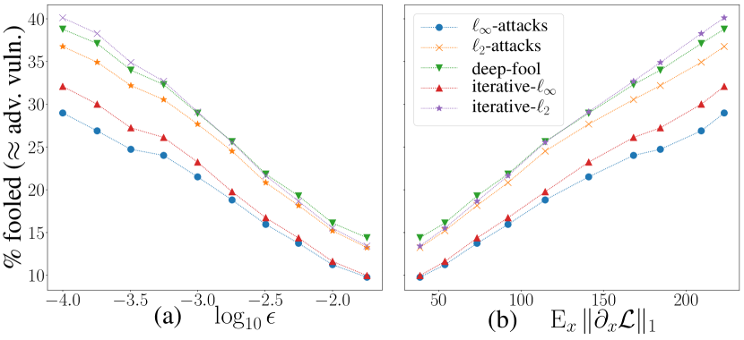
Figure 6: Same as Figure 4 but using an $\mathcal{\ell}_{2}$ threshold instead of a $\mathcal{\ell}_{\infty}$ one. Now the $\mathcal{\ell}_{2}$-based methods (deep-fool, and single-step and iterative $\mathcal{\ell}_{2}$-attacks) seem more effective than the $\mathcal{\ell}_{\infty}$ ones.

Appendix G Additional Material on the Up-Sampled CIFAR-10 Experiments of Section 4.2

G.1 Network architectures

The architecture of the CNNs used in Section 4.2 was a succession of 8 ‘convolution $\rightarrow$ batchnorm $\rightarrow$ ReLU’ layers with $64$ output channels, followed by a final full-connection to the logit-outputs. We used $2\times 2$-max-poolings after the convolutions of layers 2,4, 6 and 8, and a final max-pooling after layer 8 that fed only 1 neuron per channel to the fully-connected layer. To ensure that the convolution-kernels cover similar ranges of the images across each of the 32, 64, 128 and 256 input-resolutions, we respectively dilated all convolutions (‘à trous’) by a factor $1$, $2$, $4$ and $8$.

G.2 Additional Plots

Here we provide various additional plots computed with the networks trained in Section 4.2 on upsampled CIFAR-10 images of various sizes.

We first reproduce on Figure 7 the equivalent of Figure 1 (that compared the different regularization methods) but with each curve now representing a specific input-size instead of a regularization method. Figure 8 then analyses the evolution over training epochs of the test set performances on the up-sampled 3x256x256 CIFAR-10 images and unveils a striking discrepancy between error-rate (-damage) and cross-entropy loss (-damage): the cross-entropy clearly overfits, but the error-rate does not. This motivates a small comparison between performance at end-of-training and at early stopping (i.e. at the epochs with minimal cross-entropy loss). Figure 9 therefore merges several plots from the training curves of Figure 8 by using the epochs an implicit parameter, and compares their relation at end-of-training and after early-stopping. Figure 10 continues the comparison between end-of-training and early-stopping. Figure 11 then essentially plots the equivalent of Fig.8 but for the training-set values, showing that, contrary to the test set values, the training-error and -loss and -loss-damage decrease over training. This adversarial loss-damage appears to be much smaller on the training than on the test set, which motivates our last figure, Figure 12, that compares the training and test gradient $\mathcal{\ell}_{1}$-norms for all input resolutions. It confirms the huge discrepancy between the gradient norms on the training and test set. This suggests that, outside the training sample, and without strong regularization, the networks tend to recover their prior gradient-properties, i.e. naturally large gradients.

For detailed comments, see figures’ captions. Note that, for improved readability, Figures 8, 11 & 12 were smoothed using an exponential moving average with weight $0.9$, $0.6$ and $0.6$ respectively (higher weights $\rightarrow$ smoother).

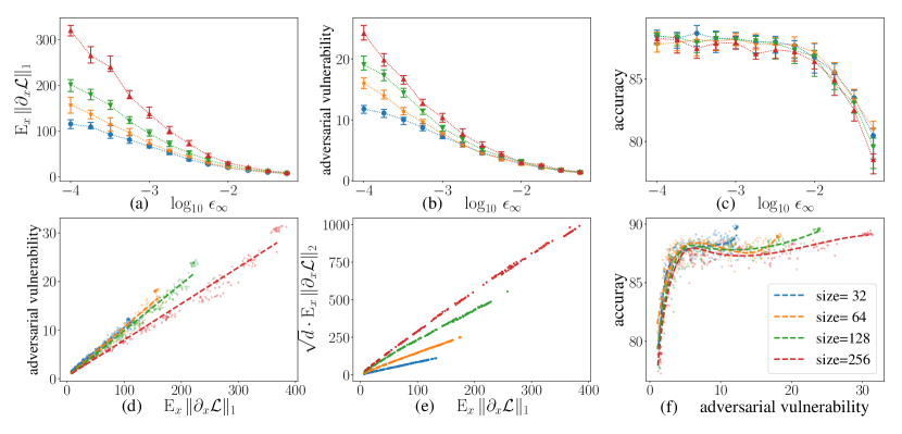
Figure 7: Equivalent of Figure 1, but with each curve representing one specific input-size (using up-sampled CIFAR-10 images) rather than one training method. Recall that all values (gradient-norms, vulnerability and accuracy) were measured over the last 20 training epochs on the test set. They appear all as an individual points on the bottom-row plots, and are summarized with errorbars on the upper-row. (d): confirms the functional- (linear-) like relation between average loss-gradient norms and adversarial vulnerability. While the slope of this relation stays unchanged for images of height and width $\leq 128$, it gets slightly dampened for size $256$. Overall, this plot confirms that first-order vulnerability (i.e. gradient-norms) is an essential part of adversarial vulnerability. (e): confirms the linear relationship between $\mathcal{\ell}_{1}$- and $\mathcal{\ell}_{2}$-gradient-norms (which explains why protecting against $\mathcal{\ell}_{\infty}$-attacks also protects against $\mathcal{\ell}_{2}$-attacks and vice-versa), but reveals that the slope does not just change like $\sqrt{d}$ with growing dimension. Figs.7a & 7b are the same than Figs.2b & 2a (main part), but with a different presentation. Figs.7c & 7f are the same than Figs.2c & 2d (see main part for comments).

Figure 8: Evolution over the training epochs of the networks’ test-set performances on the 3x256x256 up-sampled CIFAR-10 dataset. We call “adversarial error-rate” the error-rate after attack (i.e. usual error-rate plus accuracy-damage). We also divided the adversarial loss damage by the attack-threshold $\epsilon_{\infty}$ to get the same units than $\mathop{\mathbb{E}_{\bm{x}}}\left[\bm{\partial_{\scriptscriptstyle x}}\mathcal{L}\right]$ (see Fig.9 for explanations). While the usual error-rate constantly decreases on the test-set (hence showing no sign of overfitting), surprisingly, with low or no PGD-regularization, the cross-entropy loss (i.e. the training objective) severely increases after approximately 50 epochs. Moreover, the adversarial error-rate (and vulnerability/loss-damage/gradient-norms) curve has a strikingly similar shape. Hence, even though the accuracy improves, the cross-entropy overfitting still signals some form of overfitting (that could be called ‘gradient-overfitting’), which makes the network more vulnerable.

Figure 9: Relations between adversarial vulnerability, loss- and accuracy-damage, and loss-gradient norms computed on the up-sampled 3x256x256 CIFAR-10 test set images over the 20 last training epochs (blue) and at the 20 optimal early-stopping epochs (green), i.e. the 20 epochs with smallest cross-entropy test-loss. Note that these plots essentially merge different plots from Fig.8 by using the 20 end-of-training and 20 early-stopping epochs as a common implicit parameter. As in Fig.8, we divided the adversarial loss damage by the attack-threshold $\epsilon_{\infty}$. This ‘normalized’ loss damage can thus be understood as the average loss-gradient norm between an image $\bm{x}$ and its adversarial perturbation $\bm{x}+\bm{\delta}$, and can directly be compared with $\mathop{\mathbb{E}_{\bm{x}}}\left[\bm{\partial_{\scriptscriptstyle x}}\mathcal{L}\right]$. (a) Gradient norms appear to be a stable indicator for loss-damage through-out training. Note however that the gradient norms at the original input points are on average only half the size of the gradients of their surroundings. That might explain why in practice, iterative gradient regularization (e.g. PGD) is more effective than single-step regularization (e.g. FGSM). (b) Adversarial accuracy- and loss-damage are in a functional-like relationship, but which evolves over training (thus the difference between end-of-training and early-stopping). (c) Adversarial vulnerability and accuracy-damage are in a constant, almost perfectly proportional relationship. Comparing (b) and (c) suggests that the main difference between adversarial loss-damage and adversarial vulnerability comes from the difference between the $\mathcal{L}_{0/1}$- and the cross-entropy loss $\mathcal{L}$.

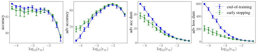
Figure 10: Network performance at early stopping versus end-of-training, for different regularization strength, on up-sampled 3x256x256 CIFAR-10 images. Training past the epochs with minimal cross-entropy test-loss might improve the final test-accuracy, but significantly increases the networks’ vulnerability. (The left-most point of each curve actually corresponds to $\epsilon_{\infty}=0.$).

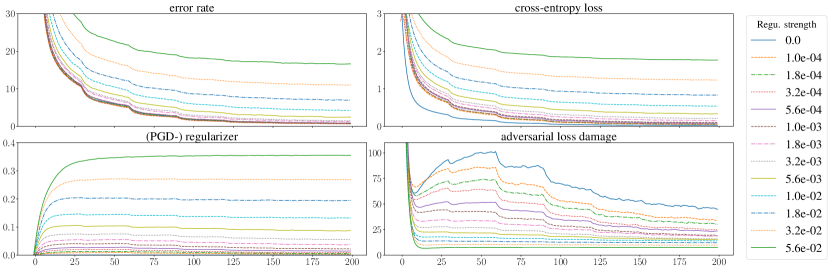
Figure 11: Evolution over the training epochs of the networks’ training-set performances on the 3x256x256 up-sampled CIFAR-10 dataset. Compare with Fig.8 for the corresponding test-set performances. Contrary to the test-set performances, error-rate, cross-entropy and adversarial loss-damage all steadily decrease (after some initialization epochs).

Figure 12: Evolution over training epochs of the average $\mathcal{\ell}_{1}$-gradient-norms on the test (top row) and training set (bottom row). There is a clear discrepancy between training and test set values: after around 50-epochs of initialization, the gradient norms constantly decrease on the training set and become dimension independent (even without regularization); on the test set however, they increase and scale like $\sqrt{d}$. This suggests that, outside the training points, and without very strong gradient regularization, the nets tend to recover their prior gradient-properties (i.e. naturally large gradients).

Appendix H Figures for the Experiments of Section 4.2 on the Custom Mini-ImageNet Dataset

Figure 13: Same as Figure 2, but using down-sampled images from our custom 12-class ‘Mini-ImageNet’ dataset (see Sec.4.2) rather than up-sampled CIFAR-10 images. Interestingly, (d) shows that PGD training finds better accuracy-vulnerability trade-offs with higher input dimensions. It is thus more effective at tackling adversarial vulnerability than a simple initial down-sampling layer that would be used to reduce the data’s dimension.

Figure 14: Same as Figure 7, but using down-sampled images from our custom 12-class ‘Mini-ImageNet’ dataset rather than up-sampled CIFAR-10 images.

References

- Amsaleg et al. (2017) Amsaleg, L., Bailey, J. E., Barbe, D., Erfani, S., Houle, M. E., Nguyen, V., and Radovanovic, M. The vulnerability of learning to adversarial perturbation increases with intrinsic dimensionality. In IEEE Workshop on Information Forensics and Security, 2017.
- Athalye et al. (2018) Athalye, A., Carlini, N., and Wagner, D. Obfuscated gradients give a false sense of security: Circumventing defenses to adversarial examples. In ICML, 2018.
- Balduzzi et al. (2017) Balduzzi, D., McWilliams, B., and Butler-Yeoman, T. Neural taylor approximations: Convergence and exploration in rectifier networks. In ICML, 2017.
- Bishop (1995) Bishop, C. M. Training with noise is equivalent to Tikhonov regularization. Neural computation, 7(1):108–116, 1995.
- Drucker & LeCun (1991) Drucker, H. and LeCun, Y. Double backpropagation increasing generalization performance. In International Joint Conference on Neural Networks, 1991.
- Gilmer et al. (2018) Gilmer, J., Metz, L., Faghri, F., Schoenholz, S. S., Raghu, M., Wattenberg, M., and Goodfellow, I. Adversarial spheres. In ICLR Workshop, 2018.
- Goodfellow et al. (2015) Goodfellow, I. J., Shlens, J., and Szegedy, C. Explaining and harnessing adversarial examples. In ICLR, 2015.
- He et al. (2015) He, K., Zhang, X., Ren, S., and Sun, J. Delving deep into rectifiers: Surpassing human-level performance on imagenet classification. In ICCV, 2015.
- Hein & Andriushchenko (2017) Hein, M. and Andriushchenko, M. Formal guarantees on the robustness of a classifier against adversarial manipulation. In NIPS, 2017.
- Huang (2000) Huang, J. Statistics of Natural Images and Models. PhD thesis, Brown University, Providence, RI, 2000.
- Krizhevsky (2009) Krizhevsky, A. Learning multiple layers of features from tiny images. Technical report, 2009.
- Lyu et al. (2015) Lyu, C., Huang, K., and Liang, H.-N. A unified gradient regularization family for adversarial examples. In ICDM, 2015.
- Madry et al. (2018) Madry, A., Makelov, A., Schmidt, L., Tsipras, D., and Vladu, A. Towards deep learning models resistant to adversarial attacks. In ICLR, 2018.
- Moosavi-Dezfooli et al. (2016) Moosavi-Dezfooli, S.-M., Fawzi, A., and Frossard, P. DeepFool: A simple and accurate method to fool deep neural networks. In CVPR, 2016.
- Neal (1996) Neal, R. M. Bayesian Learning for Neural Networks, volume 118 of Lecture Notes in Statistics. Springer, 1996.
- Ollivier (2014) Ollivier, Y. Auto-encoders: Reconstruction versus compression. arXiv:1403.7752, 2014.
- Rauber et al. (2017) Rauber, J., Brendel, W., and Bethge, M. Foolbox v0.8.0: A Python toolbox to benchmark the robustness of machine learning models. arXiv:1707.04131, 2017.
- Rifai et al. (2011) Rifai, S., Vincent, P., Muller, X., Glorot, X., and Bengio, Y. Contractive auto-encoders: Explicit invariance during feature extraction. In ICML, 2011.
- Ross & Doshi-Velez (2018) Ross, A. S. and Doshi-Velez, F. Improving the adversarial robustness and interpretability of deep neural networks by regularizing their input gradients. In AAAI, 2018.
- Schmidt et al. (2018) Schmidt, L., Santurkar, S., Tsipras, D., Talwar, K., and Mądry, A. Adversarially robust generalization requires more data. arXiv:1804.11285, 2018.
- Shafahi et al. (2019) Shafahi, A., Huang, W. R., Studer, C., Feizi, S., and Goldstein, T. Are adversarial examples inevitable? In ICLR, 2019.
- Sinha et al. (2018) Sinha, A., Namkoong, H., and Duchi, J. Certifiable distributional robustness with principled adversarial training. In ICLR, 2018.
- Soudry et al. (2018) Soudry, D., Hoffer, E., Nacson, M. S., Gunasekar, S., and Srebro, N. The implicit bias of gradient descent on separable data. JMLR, 19(70):1–57, 2018.
- Yuan et al. (2017) Yuan, X., He, P., Zhu, Q., Bhat, R. R., and Li, X. Adversarial examples: Attacks and defenses for deep learning. arXiv:1712.07107, 2017.