Molecular diffusion of stable water isotopes in polar firn as a proxy for past temperatures

Abstract

Polar precipitation archived in ice caps contains information on past temperature conditions. Such information can be retrieved by measuring the water isotopic signals of $\delta{}^{18}\mathrm{O}$ and $\delta\mathrm{D}$ in ice cores. These signals have been attenuated during densification due to molecular diffusion in the firn column, where the magnitude of the diffusion is isotopologoue specific and temperature dependent. By utilizing the differential diffusion signal, dual isotope measurements of $\delta{}^{18}\mathrm{O}$ and $\delta\mathrm{D}$ enable multiple temperature reconstruction techniques. This study assesses how well six different methods can be used to reconstruct past surface temperatures from the diffusion-based temperature proxies. Two of the methods are based on the single diffusion lengths of $\delta{}^{18}\mathrm{O}$ and $\delta\mathrm{D}$, three of the methods employ the differential diffusion signal, while the last uses the ratio between the single diffusion lengths. All techniques are tested on synthetic data in order to evaluate their accuracy and precision. We perform a benchmark test to thirteen high resolution Holocene data sets from Greenland and Antarctica, which represent a broad range of mean annual surface temperatures and accumulation rates. Based on the benchmark test, we comment on the accuracy and precision of the methods. Both the benchmark test and the synthetic data test demonstrate that the most precise reconstructions are obtained when using the single isotope diffusion lengths, with precisions of approximately $1.0\,^{\mathrm{o}}\mathrm{C}$. In the benchmark test, the single isotope diffusion lengths are also found to reconstruct consistent temperatures with a root-mean-square-deviation of $0.7\,^{\mathrm{o}}\mathrm{C}$. The techniques employing the differential diffusion signals are more uncertain, where the most precise method has a precision of $1.9\,^{\mathrm{o}}\mathrm{C}$. The diffusion length ratio method is the least precise with a precision of $13.7\,^{\mathrm{o}}\mathrm{C}$. The absolute temperature estimates from this method are also shown to be highly sensitive to the choice of fractionation factor parameterization.

I Introduction

Polar precipitation stored for thousands of years in the ice caps of Greenland and Antarctica contains unique information on past climatic conditions. The isotopic composition of polar ice, commonly expressed through the $\delta$ notation has been used as a direct proxy of the relative depletion of a water vapor mass in its journey from the evaporation site to the place where condensation takes place [20, 44]. Additionally, for modern times, the isotopic signal of present day shows a good correlation with the temperature of the cloud at the time of precipitation [14, 15] and as a result it has been proposed and used as a proxy of past temperatures [34, 33, 29].

The use of the isotopic paleothermometer presents some notable limitations. The modern day linear relationship between $\delta{}^{18}\mathrm{O}$ and temperature commonly referred to as the “spatial slope” may hold for present conditions, but studies based on borehole temperature reconstruction [12, 28] as well as the thermal fractionation of the $\delta{}^{15}\mathrm{N}$ signal in polar firn [53, 52] have independently underlined the inaccuracy of the spatial isotope slope when it is extrapolated to past climatic conditions. Even though qualitatively the $\delta{}^{18}\mathrm{O}$ signal comprises past temperature information, it fails to provide a quantitative picture on the magnitudes of past climatic changes.

[27, 64] and [31] set the foundations for the quantitative description of the diffusive processes the water isotopic signal undergoes in the porous firn layer from the time of deposition until pore close–off. Even though the main purpose of [31] was to investigate how to reconstruct the part of the signal that was attenuated during the diffusive processes, the authors make a reference to the possibility of using the assessment of the diffusive rates as a proxy for past firn temperatures.

The temperature reconstruction method based on isotope firn diffusion requires data of high resolution. Moreover, if one would like to look into the differential diffusion signal, datasets of both $\delta{}^{18}\mathrm{O}$ and $\delta\mathrm{D}$ are required. Such data sets have until recently not been easy to obtain especially due to the challenging nature of the $\delta\mathrm{D}$ analysis [7, 59]. With the advent of present commercial high–accuracy, high–precision Infra-Red spectrometers [11, 9], simultaneous measurements of $\delta{}^{18}\mathrm{O}$ and $\delta\mathrm{D}$ have become easier to obtain. Coupling of these instruments to Continuous Flow Analysis systems [23, 41, 19, 32] can also result in measurements of ultra–high resolution, a necessary condition for accurate temperature reconstructions based on water isotope diffusion.

A number of existing works have presented past firn temperature reconstructions based on water isotope diffusion. [54] and [24] used high resolution isotopic datasets from the NorthGRIP ice core [45]. The first study makes use of the differential diffusion signal, utilizing spectral estimates of high–resolution dual $\delta{}^{18}\mathrm{O}$ and $\delta\mathrm{D}$ datasets covering the GS–1 and GI–1 periods in the NorthGRIP ice core [50]. The second study presents a combined temperature and accumulation history of the past 16,000 years based on the power spectral density (PSD hereafter) signals of high resolution $\delta{}^{18}\mathrm{O}$ measurements of the NorthGRIP ice core. More recently, [58] introduced a slightly different approach for reconstructing the differential diffusion signal and testing it on dual $\delta{}^{18}\mathrm{O}$, $\delta\mathrm{D}$ high resolution data from the EDML ice core [46]. By artificially forward–diffusing the $\delta\mathrm{D}$ signal the authors estimate differential diffusion rates by maximizing the correlation between the $\delta{}^{18}\mathrm{O}$ and $\delta\mathrm{D}$ signal. In this work we attempt to test the various approaches in utilizing the temperature reconstruction technique.

We use synthetic, as well as real ice core data sets that represent Holocene conditions from a variety of drilling sites on Greenland and Antarctica. Our objective is to use data sections that originate from parts of the core as close to present day as possible. By doing this we aim to minimize possible uncertainties and biases in the ice flow thinning adjustment that is required for temperature interpretation of the diffusion rate estimates. Such a bias has been shown to exist for the NorthGRIP ice core [24], most likely due to the [16] ice flow model overestimating the past accumulation rates for the site. In order to include as much data as possible, approximately half of the datasets used here have an age of 9-10 ka. This age coincides with the timing of the early Holocene Climate Optimum around 5-9 ka (HCO hereafter). For Greenlandic drill sites, temperatures were up to $3\,^{\mathrm{o}}$C warmer than present day during the HCO [13]. Another aspect of this study is that it uses water isotopic data sets of $\delta{}^{18}\mathrm{O}$ and $\delta\mathrm{D}$ measured using different analytical techniques, namely Isotope Ratio Mass Spectroscopy (IRMS hereafter) as well as Cavity Ring Down Spectroscopy (CRDS hereafter). Two of the data sets presented here were obtained using Continuous Flow Analysis (CFA hereafter) systems tailored for water isotopic analysis [23]. All data sections are characterized by a very high sampling resolution typically of $5\,\mathrm{cm}$ or better.

II Theory

II-A Diffusion of water isotope signals in firn

The porous medium of the top $60-80\,\mathrm{m}$ of firn allows for a molecular diffusion process that attenuates the water isotope signal from the time of deposition until pore close–off. The process takes place in the vapor phase and it can be described by Fick’s second law as (assuming that the water isotope ratio signal ($\delta$) approximates the concentration):

$$\frac{\partial\delta}{\partial t}=D\left(t\right)\frac{\partial^{2}\delta}{\partial z^{2}}-\dot{\varepsilon}_{z}\left(t\right)z~{}\frac{\partial\delta}{\partial z}\enspace$$ (1)

where $D\left(t\right)$ is the diffusivity coefficient, $\dot{\varepsilon}_{z}\left(t\right)$ the vertical strain rate and $z$ is the vertical axis of a coordinate system, with its origin being fixed within the considered layer. The attenuation of the isotopic signal results in loss of information. However, the dependence of $\dot{\varepsilon}_{z}\left(t\right)$ and $D\left(t\right)$ on temperature and accumulation presents the possibility of using the process as a tool to infer these two paleoclimatic parameters. A solution to Eq. 1 can be given by the convolution of the initial isotopic profile $\delta^{\prime}$ with a Gaussian filter $\mathcal{G}$ as:

$$\delta\left(z\right)=\mathcal{S}\left(z\right)\left[\delta^{\prime}\left(z\right)\ast\mathcal{G}\left(z\right)\right]$$ (2)

where the Gaussian filter is described as:

$$\mathcal{G}\left(z\right)=\frac{1}{\sigma\sqrt{2\pi}}\,e^{\frac{-z^{2}}{2\sigma^{2}}}\enspace,$$ (3)

and $\mathcal{S}$ is the total thinning of the layer at depth $z$ described by

$$\mathcal{S}\left(z\right)=e^{\int_{0}^{z}\dot{\varepsilon}_{z}\left(z^{\prime}\right)\mathrm{d}z^{\prime}}\enspace.$$ (4)

In Eq. 3, the standard deviation term $\sigma^{2}$ represents the average displacement of a water molecule along the z–axis and is commonly referred to as the diffusion length. The $\sigma^{2}$ quantity is a direct measure of diffusion and its accurate estimate is critical to any attempt of reconstructing temperatures that are based on the isotope diffusion thermometer. The diffusion length is directly related to the diffusivity coefficient and the strain rate (as the strain rate is approximately proportional to the densification rate in the firn column) and it can therefore be regarded as a measure of firn temperature.

The differential equation describing the evolution of $\sigma^{2}$ with time is given by [27]:

$$\frac{\mathrm{d}\sigma^{2}}{\mathrm{d}t}-2\,\dot{\varepsilon}_{z}\!\left(t\right)\sigma^{2}=2D\!\left(t\right)\enspace.$$ (5)

In the case of firn the following approximation can be made for the strain rate:

$$\dot{\varepsilon}_{z}\left(t\right)\approx-\frac{\mathrm{d\rho}}{\,\,\,\mathrm{dt}}\,\frac{\,1\,}{\,\rho\,},$$ (6)

with $\rho$ representing the density. Then for the firn column, Eq. 5 can be solved hereby yielding a solution for $\sigma^{2}$:

$$\sigma^{2}\left(\rho\right)=\frac{\,1\,}{\rho^{2}}\int_{\rho_{o}}^{\rho}2\rho^{2}{\left(\frac{\mathrm{d}\rho}{\mathrm{d}t}\right)}^{-1}\!D\!\left(\rho\right)\,\mathrm{d}\rho,$$ (7)

where $\rho_{o}$ is the surface density. Under the assumption that the diffusivity coefficient $D\left(\rho\right)$ and the densification rate $\frac{\mathrm{d}\rho}{\mathrm{d}t}$ are known, integration from surface density $\rho_{o}$ to the close–off density $\rho_{co}$ can be performed yielding a model based estimate for the diffusion length. In this work we make use of the Herron–Langway densification model (H–L hereafter) and the diffusivity rate parametrization introduced by [31] (Supplementary Online Material (SOM) Sec. S1). $\frac{\mathrm{d}\rho}{\mathrm{d}t}$ depends on temperature and overburden pressure and $D\left(\rho\right)$ depends on temperature and firn connectivity. Our implementation of Eq. 7 includes a seasonal temperature signal that propagates down in the firn (SOM Sec. S2). The seasonal temperature variation affects the firn diffusion length nonlinearly in the upper $10-12\,\mathrm{m}$ due to the saturation vapor pressure’s exponential dependence on temperature.

In Fig. 1 we evaluate Eq. 7 for all three isotopic ratios of water ($\delta{}^{18}\mathrm{O}$, $\delta{}^{17}\mathrm{O}$, $\delta\mathrm{D}$) using boundary conditions characteristic of ice core sites from central Greenland and the East Antarctic Ice Cap. In Fig. 1, the transition between zone 1 and zone 2 densification (at the critical density $\rho_{\mathrm{c}}=550\,\mathrm{kgm}^{-3}$) is evident as a kink in both the densification and diffusion model. For the first case we consider cold and dry conditions (case A hereafter) representative of Antarctic ice coring sites (e.g. Dome C, Vostok) with a surface temperature $T_{\mathrm{sur}}=-55\,^{\circ}\mathrm{C}$ and annual accumulation $A=0.032\;\mathrm{myr^{-1}\,ice\,eq.}$ For the second case we consider relatively warm and humid conditions (case B hereafter) representative of central Greenlandic ice coring sites (e.g. GISP2, GRIP, NorthGRIP) with a surface temperature $T_{\mathrm{sur}}=-29\,^{\circ}\mathrm{C}$ and annual accumulation $A=0.22\;\mathrm{myr^{-1}\,ice\,eq.}$ The general impact of surface temperature and accumulation rate on the firn diffusion length can be seen in Fig. 2.

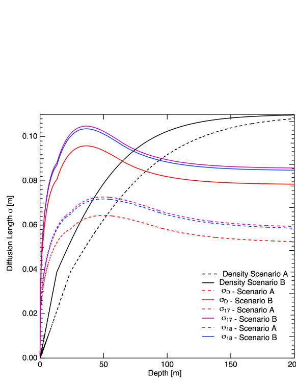
Figure 1: Diffusion length and density profiles (black) for case A (dashed lines: $T_{\mathrm{sur}}=-55\,^{\circ}\mathrm{C}$, $A=0.032\;\mathrm{myr^{-1}}$) and B (solid curves: $T_{\mathrm{sur}}=-29\,^{\circ}\mathrm{C}$, $A=0.22\;\mathrm{myr^{-1}}$). The increase in diffusion of the $\delta{}^{18}\mathrm{O}$ (blue color), $\delta{}^{17}\mathrm{O}$ (purple color) and $\delta\mathrm{D}$ (red color) isotope signals are partially due to the compaction of the firn which moves the ice closer together.

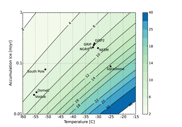
Figure 2: Modeled firn diffusion lengths [cm] for $\delta^{18}$O as a function of temperature and accumulation rate (with $\rho_{\mathrm{co}}=804\mathrm{kgm}^{-3}$ and $\rho_{\mathrm{o}}=330\mathrm{kgm}^{-3}$) from [24]. The contours indicate lines of constant diffusion length and the colorbar represents the diffusion length in cm. Here the combined impact of temperature and accumulation rate on the diffusion length is evident; while warm temperatures induce high diffusion lengths, a high accumulation rate reduces the diffusion length estimate. The firn diffusion lengths corresponding to a few ice core sites are plotted as a reference.

II-B Isotope diffusion in the solid phase

Below the close-off depth, diffusion occurs in solid ice driven by the isotopic gradients within the lattice of the ice crystals. This process is several orders of magnitude slower than firn diffusion. Several studies exist that deal with the estimate of the diffusivity coefficient in ice [26, 8, 17, 48, 38]. The differences resulting from the various diffusivity coefficients are small and negligible for the case of our study (for a brief comparison between the different parameterizations, the reader is referred to [24]). As done before by other similar firn diffusion studies [31, 54, 24] we make use of the parametrization given in [48] as:

$$D_{\mathrm{ice}}=9.2\cdot 10^{-4}\cdot\exp\left(-\frac{7186}{T}\right)\mathrm{m^{2}s^{-1}}.$$ (8)

Assuming that a depth–age scale as well as a thinning function are available for the ice core a solution for the ice diffusion length is given by (SOM Sec. S3 for details):

$$\sigma_{\mathrm{ice}}^{2}\!\left(t^{\prime}\right)=S\!\left(t^{\prime}\right)^{2}\,\int_{0}^{t^{\prime}}2D_{\mathrm{ice}}\!\left(t\right)S\!\left(t\right)^{-2}\,\mathrm{d}t.$$ (9)

In Fig. 3 we have calculated ice diffusion lengths for four different cores (NGRIP, NEEM, Dome C, EDML). For the calculation of $D_{\mathrm{ice}}$ we have used the borehole temperature profile of each core and assumed a steady state condition. As the temperature of the ice increases closer to the bedrock, $\sigma_{\mathrm{ice}}$ increases nonlinearly due to $D_{\mathrm{ice}}$ exponential temperature dependence. When approaching these deeper parts of the core, the warmer ice temperatures enhance the effect of ice diffusion which then becomes an important and progressively dominating factor in the calculations. For the special case of the Dome C core (with a bottom age exceeding 800,000 years), $\sigma_{\mathrm{ice}}$ reaches values as high as 15 $\mathrm{cm}$.

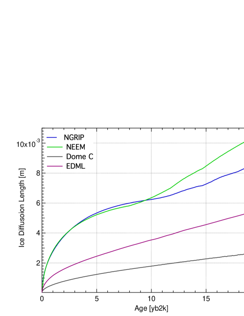
Figure 3: The ice diffusion length plotted with respect to age [b2k] for some selected sites from Greenland (NGRIP and NEEM) and Antarctica (Dome C and EDML).

III Reconstructing firn temperatures from ice core data

Here we outline the various temperature reconstruction techniques that can be employed for paleotemperature reconstructions. In order to avoid significant overlap with previously published works e.g. [27, 31, 54, 24, 58] we occasionally point the reader to any of the latter or/and refer to specific sections in the SOM. We exemplify and illustrate the use of various techniques using synthetic data prepared such that they resemble two representative regimes of ice coring sites on the Greenland summit and the East Antarctic Plateau.

III-A The single isotopologue diffusion

As shown in Eq. 2, the impact of the diffusion process can be mathematically described as a convolution of the initial isotopic profile with a Gaussian filter. A fundamental property of the convolution operation is that it is equivalent to multiplication in the frequency domain. The transfer function for the diffusion process will be given by the Fourier transform of the Gaussian filter that will itself be a Gaussian function described by [1, 24]:

$$\mathfrak{F}[\mathcal{G}(z)]=\hat{\mathcal{G}}={e}^{\frac{-k^{2}\sigma^{2}}{2}}{}\enspace.$$ (10)

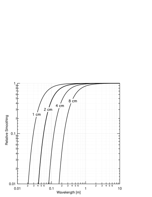
Figure 4: The smoothing effect of the diffusion transfer function demonstrated on a range of different wavelengths for $\sigma=1,\,2,\,4\;\mathrm{and}\;8\;\mathrm{cm}$.

In Eq. 10, $k=2\pi f$ where $f$ is the frequency of the isotopic time series. In Fig. 4 we illustrate the effect of the diffusion transfer function on a range of wavelengths for $\sigma=1,\,2,\,4\;\mathrm{and}\;8\;\mathrm{cm.}$ Frequencies corresponding to wavelengths on the order of $50\,\mathrm{cm}$ and above remain largely unaltered while signals with wavelengths shorter than $20\,\mathrm{cm}$ are heavily attenuated.

A data-based estimate of the diffusion length $\sigma$ can be obtained by looking at the power spectrum of the diffused isotopic time series. Assuming a noise signal $\eta\left(k\right)$, Eq. 10 provides a model describing the power spectrum as:

$$P_{s}=P_{0}(k){e}^{-k^{2}\sigma^{2}}+{|\hat{\eta}\left(k\right)|}^{2},\indent f\in\left[0,f_{\mathrm{Nq}}\right]$$ (11)

where $f_{\mathrm{Nq}}=1/\left(2\Delta\right)$ is the Nyquist frequency that is defined by the sampling resolution $\Delta$. $P_{0}(k)$ is the spectral density of the compressed profile without diffusion. It is assumed independent of $k$ (now $P_{0}$) due to the strong depositional noise encountered in high resolution $\delta$ ice core series [31]. Theoretically $|\hat{\eta}(k)|^{2}$ refers to white measurement noise. As we will show later, real ice core data sometimes have a more red noise behavior. A generalized model for the noise signal can be described well by autoregressive process of order 1 (AR-1). Its power spectral density is defined as [36]:

$$|\hat{\eta}(k)|^{2}=\frac{\sigma_{\mathrm{\eta}}^{2}\Delta}{\left|1-a_{1}\exp{\left(-ik\Delta\right)}\right|^{2}}{},$$ (12)

where $a_{1}$ is the AR-1 coefficient and $\sigma_{\mathrm{\eta}}^{2}$ is the variance of the noise signal.

In Fig. 5, an example of power spectra based on a synthetic time series is shown. A description of how the synthetic time series is generated is provided in SOM Sec. S4. The diffusion length used for the power spectrum in Fig. 5 is equal to $8.50\,\mathrm{cm}$. The spectral estimate of the time series $\mathbb{P}_{s}$ is calculated using Burg’s spectral estimation method [36] and specifically the algorithm presented in [2]. Using a least–squares approach we optimize the fit of the model $P_{s}$ to the data-based $\mathbb{P}_{s}$ by varying the four parameters $P_{0}$, $\sigma$, $a_{1}$ and $\sigma_{\mathrm{\eta}}^{2}$. In the case of Fig. 5, the $|P_{s}-\mathbb{P}_{s}|^{2}$ least squares optimization resulted in $P_{0}=0.32\,\permil^{2}\cdot\mathrm{m}$, $\sigma=8.45\,\mathrm{cm}$, $a_{1}=0.05$ and $\sigma_{\mathrm{\eta}}^{2}=0.005\,\permil^{2}$.

Assuming a diffusion length $\widehat{\sigma}_{i}^{2}$ is obtained for depth $z_{i}$ by means of $|P_{s}-\mathbb{P}_{s}|^{2}$ minimization, one can calculate the equivalent diffusion length at the bottom of the firn column $\sigma^{2}_{\mathrm{firn}}$ in order to estimate firn temperatures by means of Eq. 7. In order to do this, one needs to take into account three necessary corrections - (1) sampling diffusion, (2) ice diffusion and (3) thinning. The first concerns the artifactually imposed diffusion due to the sampling of the ice core. In the case of a discrete sampling scheme with resolution $\Delta$ the additional diffusion length is (SOM Sec. S5 for derivation):

$$\sigma^{2}_{\mathrm{dis}}=\frac{2\Delta^{2}}{\pi^{2}}\ln{\left(\frac{\pi}{2}\right)}.$$ (13)

In the case of high resolution measurements carried out with CFA measurement systems, there exist a number of ways to characterize the sampling diffusion length. Typically the step or impulse response of the CFA system can be measured yielding a Gaussian filter specific for the CFA system [23, 41, 19, 32]. The Gaussian filter can be characterized by a diffusion length $\sigma^{2}_{\mathrm{cfa}}$ that can be directly used to perform a sampling correction. The second correction concerns the ice diffusion as described in Sec. II-B. The quantities $\sigma^{2}_{\mathrm{ice}}$ and $\sigma^{2}_{\mathrm{dis}}$ can be subtracted from $\widehat{\sigma}_{i}^{2}$ yielding a scaled value of $\sigma^{2}_{\mathrm{firn}}$ due to ice flow thinning. As a result, we can finally obtain the diffusion length estimate at the bottom of the firn column $\sigma^{2}_{\mathrm{firn}}$ (in meters of ice eq.):

$$\sigma^{2}_{\text{firn}}=\frac{\widehat{\sigma}_{i}^{2}-\sigma^{2}_{\text{dis}}-\sigma^{2}_{\text{ice}}}{{\mathcal{S}(z)}^{2}}.$$ (14)

Subsequently, a temperature estimate can be obtained by numerically finding the root of (for a known $A(z)$):

$$\left(\frac{\rho_{co}}{\rho_{i}}\right)^{2}\sigma^{2}(\rho=\rho_{\mathrm{co}},T(z),A(z))-\sigma^{2}_{\text{firn}}=0$$ (15)

where $\sigma^{2}$ is the result of the integration in Eq. 7 from surface to close–off density ($\rho_{o}\rightarrow\rho_{\mathrm{co}}$). In this work we use a Newton-Raphson numerical scheme [47] for the calculation of the root of the equation.

The accuracy of the $\sigma^{2}_{\text{firn}}$ estimation and subsequently of the temperature reconstruction obtained based on it, depends on the three correction terms $\sigma^{2}_{\mathrm{ice}}$, $\sigma^{2}_{\mathrm{dis}}$ and the ice flow thinning $\mathcal{S}(z)$. For relatively shallow depths where $\sigma^{2}_{\mathrm{ice}}$ is relatively small compared to $\widehat{\sigma}_{i}^{2}$, ice diffusion can be accounted for with simple assumptions on the borehole temperature profile and the ice flow. In a similar way, $\sigma^{2}_{\mathrm{dis}}$ is a well constrained parameter and depends only on the sampling resolution $\Delta$ for discrete sampling schemes or the smoothing of the CFA measurement system.

Equation 14 reveals an interesting property of the single isotopologue temperature estimation technique. As seen, the result of the $\sigma^{2}_{\mathrm{firn}}$ calculation depends strongly on the ice flow thinning quantity $\mathcal{S}(z)^{2}$. Possible errors in the estimation of $\mathcal{S}(z)^{2}$ due to imperfections in the modelling of the ice flow will inevitably be propagated to the $\sigma^{2}_{\mathrm{firn}}$ value thus biasing the temperature estimation. Even though this appears to be a disadvantage of the method, in some instances, it can be a useful tool for assessing the accuracy of ice flow models. Provided that for certain sections of the ice core there is a temperature estimate available based on other reconstruction methods (borehole thermometry, $\delta{}^{15}\mathrm{N}$/ $\delta{}^{40}\mathrm{Ar}$) it is possible to estimate ice flow induced thinning of the ice core layers. Following this approach [24] proposed a correction in the existing accumulation rate history for the NorthGRIP ice core.

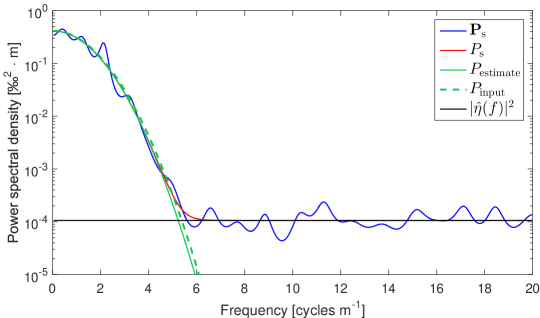
Figure 5: PSD of a synthetic $\delta{}^{18}\mathrm{O}$ time series plotted with respect to frequency (blue curve). The red curve represents the complete model fit (Eq. 11). The green dashed curve represents the input diffusion and the the solid green curve represents the estimated diffusion length of the signal (uncorrected for sampling diffusion). The black curve represents the noise part of the fit.

The annual spectral signal interference

Depending on the ice core site temperature and accumulation conditions, spectral signatures of an annual isotopic signal can be apparent as a peak located at the frequency range that corresponds to the annual layer thickness. The resulting effect of such a spectral signature, is the artifactual biasing of the diffusion length estimation towards lower values and thus colder temperatures. Figure 6 shows the PSD of the $\delta$D series for a mid Holocene section from the GRIP ice core (drill site characteristics in Table III). A prominent spectral feature is visible at $f\approx 6\,\mathrm{cycles\,m^{-1}}$. This frequency is comparable to the expected frequency of the annual signal at $6.1\,\mathrm{cycles\,m^{-1}}$ as estimated from the annual layer thickness reconstruction of the GICC05 timescale [62].

In order to evade the influence of the annual spectral signal on the diffusion length estimation, we propose the use of a weight function $w(f)$ in the spectrum as:

$$w(f)=\left\{\begin{array}[]{ll}0&f_{\lambda}-\mathrm{d}f_{\lambda}\leq f\leq f_{\lambda}+\mathrm{d}f_{\lambda}\\ 1&f<f_{\lambda}-\mathrm{d}f_{\lambda},f>f_{\lambda}+\mathrm{d}f_{\lambda}\end{array}\right.{}$$ (16)

where $f_{\lambda}$ is the frequency of the annual layer signal based on the reconstructed annual layer thickness $\lambda$ and $\mathrm{d}f_{\lambda}$ is the range around the frequency $f_{\lambda}$ at which the annual signal is detectable. The weight function is multiplied with the optimization norm $|P_{s}-\mathbb{P}_{s}|^{2}$. Figure 6 also illustrates the effect of the weight function on the estimation of $P_{s}$ and subsequently the diffusion length value. When the weight function is used during the optimization process, there is an increase in the diffusion length value by 0.3 cm, owing essentially to the exclusion of the annual signal peak from the minimization of $|P_{s}-\mathbb{P}_{s}|^{2}$. While the value of $f_{\lambda}$ can be roughly predicted, the value of $\mathrm{d}f_{\lambda}$ usually requires visual inspection of the spectrum.

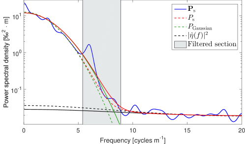
Figure 6: The interference of the annual spectral signal is seen in the PSD of the $\delta\mathrm{D}$ GRIP mid Holocene section. The regular fit is represented by the solid lines and the dashed lines represent the case where the weight function $w(f)$ has filtered out this artifactual bias.

III-B The differential diffusion signal

A second-order temperature reconstruction technique is possible based on the differential signal between $\delta{}^{18}\mathrm{O}$ and $\delta\mathrm{D}$. Due to the difference in the fractionation factors and the air diffusivities between the oxygen and deuterium isotopologues, a differential diffusion signal is created in the firn column. Based on the calculation of the diffusion lengths presented in Fig. 1 we then compute the differential diffusion lengths ${}^{17}\Delta\sigma^{2}$ and ${}^{18}\Delta\sigma^{2}$ where

$${}^{17}\Delta\sigma^{2}=\sigma^{2}_{17}-\sigma^{2}_{\mathrm{D}}\mathrm{\,\,\,and\,\,}{}^{18}\Delta\sigma^{2}=\sigma^{2}_{18}-\sigma^{2}_{\mathrm{D}}.$$ (17)

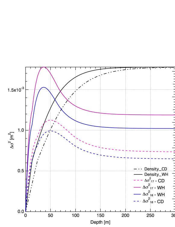
Figure 7: Differential diffusion length profiles for cases A (dashed lines) and B (solid lines) for ${}^{18}\Delta\sigma^{2}$ (blue) and ${}^{17}\Delta\sigma^{2}$ (purple). The density profiles are given in black.

As it can be seen in Fig. 7 the differential diffusion length signal is slightly larger for the case of ${}^{17}\Delta\sigma^{2}$ when compared to ${}^{18}\Delta\sigma^{2}$.

One obvious complication of the differential diffusion technique is the requirement for dual measurements of the water isotopologues, preferably performed on the same sample. The evolution of IRMS techniques targeting the analysis of $\delta\mathrm{D}$ [7, 59, 21, 6] in ice cores has allowed for dual isotopic records at high resolutions. With the advent of CRDS techniques and their customization for CFA measurements, simultaneous high resolution measurements of both $\delta{}^{18}\mathrm{O}$ and $\delta\mathrm{D}$ have become a routine procedure.

The case of $\delta{}^{17}\mathrm{O}$ is more complicated as the greater abundance of ¹³C than ¹⁷O rules out the possibility for an IRMS measurement at mass/charge ratio ($m/z$) of 45 or 29 using CO₂ equilibration or reduction to CO respectively. Alternative approaches that exist include the electrolysis method with CuSO₄ developed by [42] as well as the fluorination method presented by [3] and implemented by [5] for dual-inlet IRMS systems. These techniques target the measurement of the ¹⁷O_excess parameter and are inferior for $\delta{}^{17}\mathrm{O}$ measurements at high precision and have a very low sample throughput. As a result, high resolution $\delta{}^{17}\mathrm{O}$ measurements from ice cores are currently non existent. Recent innovations however in CRDS spectroscopy [56] allow for simultaneous triple isotopic measurements of $\delta\mathrm{D}$, $\delta{}^{18}\mathrm{O}$ and $\delta{}^{17}\mathrm{O}$ in a way that a precise and accurate measurement for both $\delta{}^{17}\mathrm{O}$ and ¹⁷O_excess is possible. Therefore high resolution ice core datasets of $\delta\mathrm{D}$, $\delta{}^{18}\mathrm{O}$ and $\delta{}^{17}\mathrm{O}$ should be expected in the near future.

The following analysis is focused on the ${}^{18}\Delta\sigma^{2}$ signal but it applies equally to the ${}^{17}\Delta\sigma^{2}$. The stronger attenuation of the $\delta{}^{18}\mathrm{O}$ signal with respect to the $\delta\mathrm{D}$ signal can be visually observed in the power spectral densities of the two signals. As seen in Fig. 8 the $\mathbb{P}_{\mathrm{S18}}$ signal reaches the noise level at a lower frequency when compared to the $\mathbb{P}_{\mathrm{SD}}$ signal. At low frequencies with high signal to noise ratio we can calculate the logarithm of the ratio of the two power spectral densities as (i.e. neglecting the noise term):

$$\ln\left(\frac{P_{\mathrm{D}}}{P_{18}}\right)\approx k^{2}\left(\sigma^{2}_{18}-\sigma^{2}_{\mathrm{D}}\right)+\ln\left(\frac{P_{0_{\mathrm{D}}}}{P_{0_{18}}}\right)={}^{18}\Delta\sigma^{2}\,k^{2}+C.$$ (18)

As seen in Eq. 18 and Fig. 8 (synthetic generated $\delta{}^{18}\mathrm{O}$ and $\delta\mathrm{D}$ data as in Sec. III-A) an estimate of the ${}^{18}\Delta\sigma^{2}$ parameter can be obtained by a linear fit of $\ln\left({P_{\mathrm{D}}}/{P_{18}}\right)$ in the low frequency area, thus requiring only two parameters $({}^{18}\Delta\sigma^{2}\mathrm{\,and\,}C)$ to be tuned. An interesting aspect of the differential diffusion method, is that in contrast to the single isotopologue diffusion length, ${}^{18}\Delta\sigma^{2}_{\mathrm{firn}}$ is a quantity that is independent of the sampling and solid ice diffusion thus eliminating the uncertainties associated with these two parameters. This can be seen by simply using Eq. 14:

$${}^{18}\Delta\sigma^{2}_{\mathrm{firn}}=\frac{\hat{\sigma}_{18}^{2}-\sigma_{\mathrm{dis}}^{2}-\sigma_{\mathrm{ice}}^{2}}{\mathcal{S}(z)^{2}}-\frac{\hat{\sigma}_{\mathrm{D}}^{2}-\sigma_{\mathrm{dis}}^{2}-\sigma_{\mathrm{ice}}^{2}}{\mathcal{S}(z)^{2}}=\frac{\hat{\sigma}_{18}^{2}-\hat{\sigma}_{\mathrm{D}}^{2}}{\mathcal{S}(z)^{2}}.$$ (19)

Accurate estimates of the thinning function however still play a key role in the differential diffusion technique. One more complication of the differential diffusion technique is the selection of the frequency range in which one chooses to apply the linear regression. Often visual inspection is required in order to designate a cut-off frequency until which the linear regression can be applied. In most cases identifying the cut-off frequency, or at least a reasonable area around it is reasonably straight-forward. Though in a small number of cases, spectral features in the low frequency area seem to have a strong influence on the slope of the linear regression and thus on the ${}^{18}\Delta\sigma^{2}$. As a result, visual inspection of the regression result is always advised in order to avoid biases.

Another way of estimating the differential diffusion signal is to subtract the single diffusion spectral estimates $\sigma^{2}_{18}$ and $\sigma^{2}_{\mathrm{D}}$. Theoretically this approach should be inferior to the linear fit approach due to the fact that more degrees of freedom are involved in the estimation of $\sigma^{2}_{18}$ and $\sigma^{2}_{\mathrm{D}}$ (8 versus 2; 3 if the cutoff frequency is included). Here we will test both approaches.

Linear correlation method

An alternative way to calculate the differential diffusion signal ${}^{18}\Delta\sigma^{2}$ is based on the assumption that the initial precipitated isotopic signal presents a deuterium excess signal $\mathrm{d_{xs}}$ that is invariable with time and as a consequence of this, the correlation signal between $\delta{}^{18}\mathrm{O}$ and $\delta\mathrm{D}$ (hereafter $r_{\delta{}^{18}\mathrm{O}/\delta\mathrm{D}}$) is expected to have a maximum value at the time of deposition. The $\mathrm{d_{xs}}$ signal is defined as the deviation from the metoric water line $\mathrm{d_{xs}}=\delta\mathrm{D}-8\cdot\delta^{18}\mathrm{O}$ [10, 15]. From the moment of deposition, the difference in diffusion between the $\delta{}^{18}\mathrm{O}$ and $\delta\mathrm{D}$ signals results in a decrease of the $r_{\delta{}^{18}\mathrm{O}/\delta\mathrm{D}}$  value. Hence, diffusing the $\delta\mathrm{D}$ signal with a Gaussian kernel of standard deviation equal to ${}^{18}\Delta\sigma^{2}$ will maximize the value of $r_{\delta{}^{18}\mathrm{O}/\delta\mathrm{D}}$ [58] as shown in Fig. 9. Thus, the ${}^{18}\Delta\sigma^{2}$ value is found when the $r_{\delta{}^{18}\mathrm{O}/\delta\mathrm{D}}$ value has its maximum.

This type of estimation is independent of spectral estimates of the $\delta{}^{18}\mathrm{O}$ and $\delta\mathrm{D}$ time series and does not pose any requirements for measurement noise characterization or selection of cut-off frequencies. However uncertainties related to the densification and ice flow processes, affect this method equally as they do for the spectrally based differential diffusion temperature estimation. In this study, we test the applicability of the method on synthetic and real ice core data. We acknowledge that the assumption that the $\mathrm{d_{xs}}$ signal is constant with time is not entirely consistent with the fact that there is a small seasonal cycle in the $\mathrm{d_{xs}}$ signal [30]. It is thus likely to result in inaccuracies.

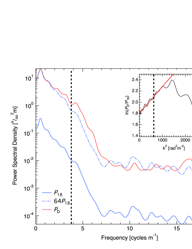
Figure 8: PSDs of synthetic $\delta{}^{18}\mathrm{O}$ (blue) and $\delta\mathrm{D}$ (red) with respect to frequency where the inner subplot shows the $\ln\left({P_{\mathrm{D}}}/{P_{18}}\right)$ relation with respect to $k^{2}$. The ${}^{18}\Delta\sigma^{2}$ value is determined from the slope of the linear fit in the subplot. The chosen cutoff frequency is marked by the vertical dashed line in both plots.

Figure 9: Correlation coefficient ($r_{\delta{}^{18}\mathrm{O}/\delta\mathrm{D}}$) between the $\delta{}^{18}\mathrm{O}$ and the forward–diffused $\delta\mathrm{D}$ series as a function of the estimated ${}^{18}\Delta\sigma^{2}$. The synthetic data represent a case A climate.

III-C The diffusion length ratio

A third way of using the diffusion lengths as proxies for temperature can be based on the calculation of the ratio of two different diffusion lengths. From Eq. 7 we can evaluate the ratio of two different isotopologues $j$ and $k$ as:

$$\frac{\sigma_{j}^{2}\left(\rho\right)}{\sigma_{k}^{2}\left(\rho\right)}=\frac{\displaystyle\frac{\,1\,}{\rho^{2}}\int 2\rho^{2}{\left(\frac{\mathrm{d}\rho}{\mathrm{d}t}\right)}^{-1}\!D_{j}\!\left(\rho\right)\,\mathrm{d}\rho}{\displaystyle\frac{\,1\,}{\rho^{2}}\displaystyle\int 2\rho^{2}{\left(\frac{\mathrm{d}\rho}{\mathrm{d}t}\right)}^{-1}\!D_{k}\!\left(\rho\right)\,\mathrm{d}\rho},$$ (20)

and by substituting the firn diffusivities as defined in SOM Sec. S1 and according to [31] we get:

$$\frac{\sigma_{j}^{2}\left(\rho\right)}{\sigma_{k}^{2}\left(\rho\right)}=\frac{D_{\mathrm{a}j}\alpha_{k}}{D_{\mathrm{a}k}\alpha_{j}}\,\frac{\displaystyle\frac{\,1\,}{\rho^{2}}\int 2\rho^{2}{\left(\frac{\mathrm{d}\rho}{\mathrm{d}t}\right)}^{-1}\!\frac{m\,p}{R\,T\,\tau}\left(\frac{\,1\,}{\,\rho\,}-\frac{\,1\,}{\,\rho_{\mathrm{ice}}\,}\right)\,\mathrm{d}\rho}{\displaystyle\frac{\,1\,}{\rho^{2}}\int 2\rho^{2}{\left(\frac{\mathrm{d}\rho}{\mathrm{d}t}\right)}^{-1}\!\frac{m\,p}{R\,T\tau}\left(\frac{\,1\,}{\,\rho\,}-\frac{\,1\,}{\,\rho_{\mathrm{ice}}\,}\right)\,\mathrm{d}\rho}=\frac{D_{\mathrm{a}j}\alpha_{k}}{D_{\mathrm{a}k}\alpha_{j}}.$$ (21)

As a result, the ratio of the diffusion lengths is dependent on temperature through the parameterizations of the fractionation factors ($\alpha$) and carries no dependence to parameters related to the densification rates nor the atmospheric pressure. Additionally, it is a quantity that is independent of depth. Here we give the analytical expressions of all the isotopologues combinations by substituting the diffusivities and the fractionation factors:

$$\sigma^{2}_{18}/\sigma^{2}_{\mathrm{D}} =0.93274\cdot\exp(16288/T^{2}-11.839/T)$$ (22)

$$\sigma^{2}_{17}/\sigma^{2}_{\mathrm{D}} =0.933\cdot\exp(16288/T^{2}-6.263/T)$$ (23)

$$\sigma^{2}_{18}/\sigma^{2}_{17} =0.99974\cdot\exp(-5.57617/T)$$ (24)

A data-based diffusion length ratio estimate can be obtained by estimating the single diffusion length values as described in Sec. III-A and thereafter applying the necessary corrections as in Eq. 14. An interesting aspect of the ratio estimation is that it is not dependent on the ice flow thinning as seen below

$$\left(\frac{\sigma^{2}_{18}}{\sigma^{2}_{\mathrm{D}}}\right)_{\mathrm{firn}}=\frac{\hat{\sigma}^{2}_{18}-\sigma^{2}_{\mathrm{dis}}-\sigma^{2}_{\mathrm{ice}}}{\hat{\sigma}^{2}_{\mathrm{D}}-\sigma^{2}_{\mathrm{dis}}-\sigma^{2}_{\mathrm{ice}}}.$$ (25)

while the method still depends on the sampling and ice diffusion.

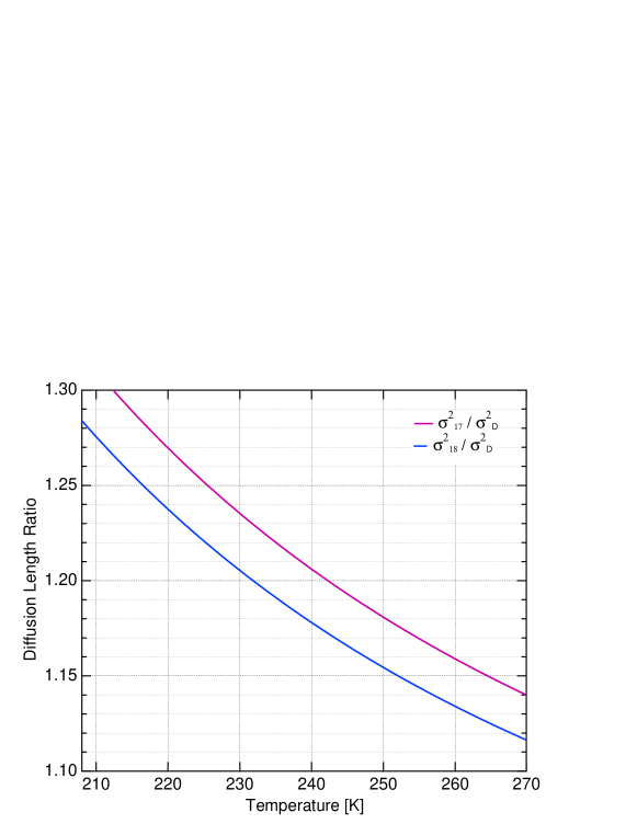
Figure 10: The diffusion length ratios $\sigma^{2}_{18}/\sigma^{2}_{\mathrm{D}}$ and $\sigma^{2}_{17}/\sigma^{2}_{\mathrm{D}}$ with respect to temperature. The $\sigma^{2}_{18}/\sigma^{2}_{17}$ is almost constant at $0.975$ and omitted here due to its very low temperature sensitivity.

IV Results

IV-A Synthetic data test

A first order test for the achievable accuracy and precision of the presented diffusion temperature reconstruction techniques can be performed using synthetic isotopic data. We generate synthetic time series of $\delta{}^{17}\mathrm{O}$, $\delta{}^{18}\mathrm{O}$ and $\delta\mathrm{D}$ using an AR-1 process and subsequently applying numerical diffusion with diffusion lengths as calculated for case A and B (as presented in Fig. 1). The time series are then sampled at a resolution of $2.5\,\mathrm{cm}$ and white measurement noise is added. Eventually, estimates of diffusion lengths for all three isotopologues are obtained using the techniques we have described in the previous sections. A more detailed description of how the synthetic data are generated is outlined in SOM Sec. S4.

The process of time series generation is repeated 500 times. For each iteration, the quantities $\sigma_{17}$, $\sigma_{18}$, $\sigma_{\mathrm{D}}$, ${}^{17}\Delta\sigma^{2}$, ${}^{18}\Delta\sigma^{2}$ and the ratios $\sigma^{2}_{18}/\sigma^{2}_{\mathrm{D}}$, $\sigma^{2}_{17}/\sigma^{2}_{\mathrm{D}}$ and $\sigma^{2}_{18}/\sigma^{2}_{17}$ are estimated. The differential diffusion signals are estimated using the three different techniques as described in Sec. III-B. We designate the subtraction technique with I, the linear regression with II and the correlation method with III. For every value of the diffusion estimates we calculate a firn temperature where the uncertainties related to the firn diffusion model ($A$, $\rho_{co}$, $\rho_{o}$, surface pressure $\mathrm{P}$, $\mathcal{S}$ and $\sigma_{ice}$ in Table I) are included. For the total of the 500 iterations we calculate a mean firn temperature $\overline{T}$, a standard deviation and a mean bias as:

$$\text{MB}=\frac{1}{N}\sum_{i=1}^{N}T_{i}-T_{\text{sur}}=\overline{T}-T_{\text{sur}},$$ (26)

where $i=1,2,\dots,N$ signifies the iteration number, $T_{i}$ is the synthetic data-based estimated temperature and $T_{\text{sur}}$ is the model forcing surface temperature for the case A and B scenarios. The results of the experiment are presented in Table II and the calculated mean biases are illustrated in Fig. 11. The diffusion length ratio approach yields very large uncertainty bars (see Table II) and thus these results are not included in Fig. 11.

TABLE I: The standard deviations of the input parameters. Most of the standard deviations are expressed as a percentage of the mean input value.

Parameter	$A$	$\rho_{co}$	$\rho_{o}$	$\mathrm{P}$	$\mathcal{S}$	$\sigma_{ice}$
Uncertainty	$\pm 5\%A_{\mathrm{mean}}$	$\pm 20\,\mathrm{kgm^{-3}}$	$\pm 30\,\mathrm{kgm^{-3}}$	$\pm 2\%\mathrm{P}_{\mathrm{mean}}$	$\pm 1\%\mathcal{S}_{\mathrm{mean}}$	$\pm 2\%\sigma_{ice_{\mathrm{mean}}}$

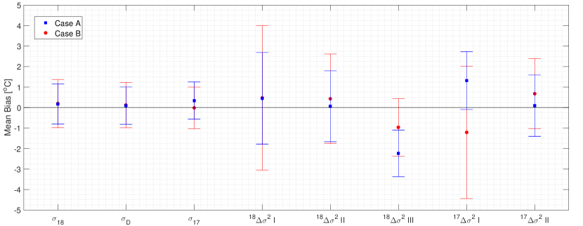
Figure 11: Mean biases for the single and differential diffusion techniques. The error bars represent 1 std of the estimated temperatures.

		Case A			Case B
	Applied diffusion	Est. diffusion	Est. T [${}^{o}\mathrm{C}$]	Applied diffusion	Est. diffusion	Est. T [${}^{o}\mathrm{C}$]
$\sigma_{18}$	$5.82$ $\mathrm{cm}$	$5.85\pm 0.14$ $\mathrm{cm}$	$-54.8\pm 1.0$	$8.50$ $\mathrm{cm}$	$8.51\pm 0.20$ $\mathrm{cm}$	$-28.8\pm 1.2$
$\sigma_{\mathrm{D}}$	$5.22$ $\mathrm{cm}$	$5.23\pm 0.12$ $\mathrm{cm}$	$-54.9\pm 0.9$	$7.86$ $\mathrm{cm}$	$7.86\pm 0.18$ $\mathrm{cm}$	$-28.9\pm 1.1$
$\sigma_{17}$	$5.90$ $\mathrm{cm}$	$5.97\pm 0.11$ $\mathrm{cm}$	$-54.7\pm 0.9$	$8.59$ $\mathrm{cm}$	$8.54\pm 0.13$ $\mathrm{cm}$	$-29.0\pm 1.0$
${}^{18}\Delta\sigma^{2}$ I	$6.6$ $\mathrm{cm^{2}}$	$6.9\pm 1.1$ $\mathrm{cm^{2}}$	$-54.6\pm 2.2$	$10.3$ $\mathrm{cm^{2}}$	$10.7\pm 2.0$ $\mathrm{cm^{2}}$	$-28.5\pm 3.5$
${}^{18}\Delta\sigma^{2}$ II	$6.6$ $\mathrm{cm^{2}}$	$6.7\pm 0.8$ $\mathrm{cm^{2}}$	$-54.9\pm 1.7$	$10.3$ $\mathrm{cm^{2}}$	$10.5\pm 1.2$ $\mathrm{cm^{2}}$	$-28.6\pm 2.2$
${}^{18}\Delta\sigma^{2}$ III	$6.6$ $\mathrm{cm^{2}}$	$5.5\pm 0.3$ $\mathrm{cm^{2}}$	$-57.2\pm 1.1$	$10.3$ $\mathrm{cm^{2}}$	$9.7\pm 0.6$ $\mathrm{cm^{2}}$	$-30.0\pm 1.4$
${}^{17}\Delta\sigma^{2}$ I	$7.5$ $\mathrm{cm^{2}}$	$8.3\pm 0.7$ $\mathrm{cm^{2}}$	$-53.7\pm 1.4$	$12.0$ $\mathrm{cm^{2}}$	$12.2\pm 2.0$ $\mathrm{cm^{2}}$	$-30.2\pm 3.2$
${}^{17}\Delta\sigma^{2}$ II	$7.5$ $\mathrm{cm^{2}}$	$7.5\pm 0.5$ $\mathrm{cm^{2}}$	$-54.9\pm 1.5$	$12.0$ $\mathrm{cm^{2}}$	$12.4\pm 1.0$ $\mathrm{cm^{2}}$	$-28.3\pm 1.7$
$\sigma^{2}_{18}/\sigma^{2}_{17}$	$0.975$	$0.960\pm 0.027$	————–	$0.977$*	$0.993\pm 0.035$*	————–
$\sigma^{2}_{18}/\sigma^{2}_{\mathrm{D}}$	$1.24$	$1.25\pm 0.04$	$-56.6\pm 11.1$	$1.17$	$1.17\pm 0.03$	$-28.2\pm 19.3$
$\sigma^{2}_{17}/\sigma^{2}_{\mathrm{D}}$	$1.28$	$1.31\pm 0.03$	$-62.8\pm 7.0$	$1.20$	$1.18\pm 0.04$	$-16.1\pm 27$

TABLE II: Simulations with synthetic data of a case A ($T_{\mathrm{sur}}=-55.0\,^{\circ}\mathrm{C}$) and B ($T_{\mathrm{sur}}=-29.0\,^{\circ}\mathrm{C}$). The diffusion lengths in the tabular are the firn diffusion lengths. Thus, this is before sampling, ice diffusion and thinning affected the input diffusion length. The estimated firn diffusion lengths are after correcting for sampling, ice diffusion and thinning (with their corresponding uncertainties).

IV-B Ice core data test

We also use a number of high resolution, high precision ice core data, in order to benchmark the diffusion temperature reconstruction techniques that we have presented. The aim of this benchmark test is to utilize the various reconstruction techniques for a range of boundary conditions that is (a) as broad as possible with respect to mean annual surface temperature and accumulation and (b) representative of existing polar ice core sites. Additionally, we have made an effort in focusing on ice core data sets that reflect conditions as close as possible to present. As a result, the majority of the data sets presented here are from relatively shallow depths. This serves a twofold purpose. Firstly, it reduces the uncertainties regarding the ice flow that are considerably larger for the deeper parts of the core. Secondly, choosing to work with data sections as close to late Holocene conditions as possible, allows for a comparison of the estimated temperature to the site’s present temperature. Although this is technically not a true comparison as the sites’ surface temperatures have very likely varied during the Holocene, we consider it as a rough estimate of each techniques accuracy. For those cases where it was not possible to obtain late Holocene isotopic time series, due to limited data availability, we have used data originating from deeper sections of the ice cores with an age of about 10ka b2k reflecting conditions of the early Holocene. In Table III we provide relevant information for each data set as well as the present temperature and accumulation conditions for each ice core site. For five out of thirteen ice core data sets, we used a weight function of $w(f_{\lambda}-0.5\leq f\leq f_{\lambda}+3)=0$ in order to remove the annual peak (see figures in SOM Sec. S6).

The data sets were produced using a variety of techniques both with respect to the analysis itself (IRMS/CRDS), as well as with respect to the sample resolution and preparation (discrete/CFA). The majority of the data sets were analyzed using CRDS instrumentation. In particular the L1102i, L2120i and L2130i variants of the Picarro CRDS analyzer were utilized for both discrete and CFA measurements of $\delta{}^{18}\mathrm{O}$ and $\delta\mathrm{D}$. The rest of the data sets were analyzed using IRMS techniques with either $\mathrm{CO}_{2}$ equilibration or high temperature carbon reduction. For the case of the NEEM early Holocene data set, we work with two data sections that span the same depth interval and consist of discretely sampled and CFA measured data respectively. Additionally, the Dome C and Dome F data sections represent conditions typical for the East Antarctic Plateau and are sampled using a different approach ($2.5\,\mathrm{cm}$ resolution discrete samples for the Dome C section and high resolution CFA measurements for the Dome F section).

In a way similar to the synthetic data test, we apply the various reconstruction techniques on every ice core data section. No reconstruction techniques involving $\delta{}^{17}\mathrm{O}$ are presented here due to lack of $\delta{}^{17}\mathrm{O}$ data. In order to achieve an uncertainty estimate for every reconstruction, we perform a sensitivity test that is based on $N=1000$ iterations. Assuming that every ice core section consists of $J$ $\delta{}^{18}\mathrm{O}$ and $\delta\mathrm{D}$ points, then a repetition is based on a data subsection with size $J^{\prime}$ that varies in the interval $\left[J/2,J\right]$. This “jittering” of the subsection size happens around the midpoint of every section and $J^{\prime}$ is drawn from a uniform distribution. Similar to the synthetic data tests, we also introduce uncertainties originating from the firn densification model, the ice flow model and ice diffusion (through the parameters: $A$, $\rho_{co}$, $\rho_{o}$, $\mathrm{P}$, $\mathcal{S}$ and $\sigma_{ice}$). For every reconstruction method and every ice core site, we calculate a mean and a standard deviation for the diffusion estimate, as well as a mean and a standard deviation for the temperature. Results are presented in Table IV. The estimated temperatures for ice cores covering the late-mid Holocene and early Holocene are shown in Fig. 12 and 13 respectively.

IV-C The fractionation factors

We also test how the choice of the parameterization of the isotope fractionation factors ($\alpha_{18}$, $\alpha_{\mathrm{D}}$) influences the reconstructed temperatures of ice core sections. This is especially relevant for temperatures below $-40\mathrm{{}^{o}C}$, as the confidence of the parameterized fractionation factors has been shown to be low for such cold temperatures [18]. The low confidence is partly a consequence of two things a) it is difficult to avoid kinetic fractionation in the measurement system and b) the water vapor pressure becomes small which makes it difficult to measure. The experiments are typically performed with a vapor source with a known isotopic composition that condenses out under controlled equilibrium conditions. For temperatures below $-40\mathrm{{}^{o}C}$, single crystals have been observed growing against the flow of vapor in the tubes and chambers of the experimental setup [18]. This indicates that the water vapor experiences kinetic fractionation which disturbs the equilibrium process. In order to avoid this, most models generally extrapolate the warmer experiments to cover colder temperatures. Such extrapolations were performed in the parameterizations of [40] ($\alpha_{18}$) and [43] ($\alpha_{\mathrm{D}}$) which we used in the firn diffusivity parameterization (SOM Sec. S1). Their experiments were conducted down to a minimum temperature of $-33\mathrm{{}^{o}C}$, and then extrapolated to colder temperatures. Similarly, [18] estimated new values of $\alpha_{18}$ and $\alpha_{\mathrm{D}}$ by measuring in the range $-40\mathrm{{}^{o}C}$ to $0\mathrm{{}^{o}C}$. Their results showed a $\alpha_{\mathrm{D}}$ parameterization that deviated significantly from that of [43]. A more recent study by [37] measured the value of $\alpha_{\mathrm{D}}$ in the range $-87\mathrm{{}^{o}C}$ to $-39\mathrm{{}^{o}C}$. Their inferred equilibrium fractionation factors required a correction for kinetic effects. By including such a correction and extrapolating to warmer temperatures, they obtained a parameterization of $\alpha_{\mathrm{D}}$ with a slightly weaker temperature dependence than that of [43]. Moreover, their $\alpha_{\mathrm{D}}$ deviated significantly from the results of [18]. Such discrepancies between the fractionation factor parameterizations underline the importance of addressing how great an impact the potential inaccuracies have on the diffusion-based temperature proxy.

In this test, the procedure followed is common to that in Sec. IV-B where a set of $N=1000$ repetitions is performed and both “jittering” of the data sets length and perturbation of input model variables takes place. The results are displayed in Fig. 14, where the temperatures resulting from the parameterizations of [40] ($\alpha_{18}$) and [43] ($\alpha_{\mathrm{D}}$) are compared to the temperatures resulting from the parameterizations of [18] ($\alpha_{18}$, $\alpha_{\mathrm{D}}$) and [37] ($\alpha_{\mathrm{D}}$). In the latter case, the parameterization of $\alpha_{18}$ from [40] is used for the dual diffusion length methods.

TABLE III: Ice core data sections and the corresponding drill site characteristic. Sources of data: [55]¹, [46]², [57]³, [22]⁴,[23]⁵. Drill site characteristic sources: [4]^a, [46, 60]^b, [63, 35]^c, [39]^d, [45, 24]^e, [31]^f, [25, 49]^g.

Site Sections	Depth	Age	Present T	A	P	Thinning	Meas.	Analysis	$\Delta$
	[$\mathrm{m}$]	[$\mathrm{kab2k}$]	[${}^{\mathrm{o}}\mathrm{C}$]	[$\mathrm{m\,ice\,yr^{-1}}$]	[$\mathrm{Atm}$]				[$\mathrm{cm}$]
GRIP midf	$753-776$	3.7	$-31.6$	0.23	0.65	0.71	$\delta$D, $\delta^{18}$O	2130	2.5
GRIP latef	$514-531$	2.4	$-31.6$	0.23	0.65	0.79	$\delta$D, $\delta^{18}$O	2130	2.5
WAIS 2005Aa,1	$120-150$	0.5	$-31.1$	0.22	0.77	0.97	$\delta^{18}$O	1102	5.0
EDMLb,2	$123-178$	1.6	$-44.6$	0.08	0.67	0.93	$\delta$D, $\delta^{18}$O	IRMS	5.0
NEEMg	$174-194$	0.8	$-29.0$	0.22	0.72	0.31	$\delta$D, $\delta^{18}$O	2120	2.5
NGRIPe	$174-194$	0.9	$-31.5$	0.20	0.67	0.49	$\delta^{18}$O	IRMS	2.5
Dome Fc,3	$302-307$	9.6	$-57.3$	0.04	0.61	0.93	$\delta$D, $\delta^{18}$O	CFA1102	0.5
Dome Cd,4	$308-318$	9.9	$-53.5$	0.04	0.65	0.93	$\delta$D, $\delta^{18}$O	IRMS	2.5
GRIP earlyf	$1449-1466$	9.4	$-31.6$	0.23	0.65	0.42	$\delta$D, $\delta^{18}$O	2130	2.5
NEEM disg,5	$1380-1392$	10.9	$-29.0$	0.22	0.72	0.31	$\delta$D, $\delta^{18}$O	2120	5.0
NEEM CFAg,5	$1382-1399$	10.9	$-29.0$	0.22	0.72	0.31	$\delta$D, $\delta^{18}$O	CFA1102	0.5
NGRIP Ie	$1300-1320$	9.1	$-31.5$	0.18	0.67	0.55	$\delta^{18}$O	IRMS	5.0
NGRIP IIe	$1300-1320$	9.1	$-31.5$	0.18	0.67	0.55	$\delta^{18}$O	IRMS	5.0

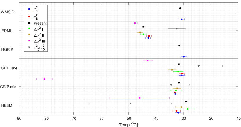
Figure 12: Late-mid Holocene section with reconstructed temperatures from the $\sigma^{2}_{18}$ (blue circles), $\sigma^{2}_{\mathrm{D}}$ (red circles), $\Delta\sigma^{2}$ I (green squares), $\Delta\sigma^{2}$ II (brown squares), $\Delta\sigma^{2}$ III (magenta squares) and ${\sigma^{2}_{18}}/{\sigma^{2}_{\mathrm{D}}}$ (grey triangles) methods. The black stars represent the present annual mean temperatures at the sites.

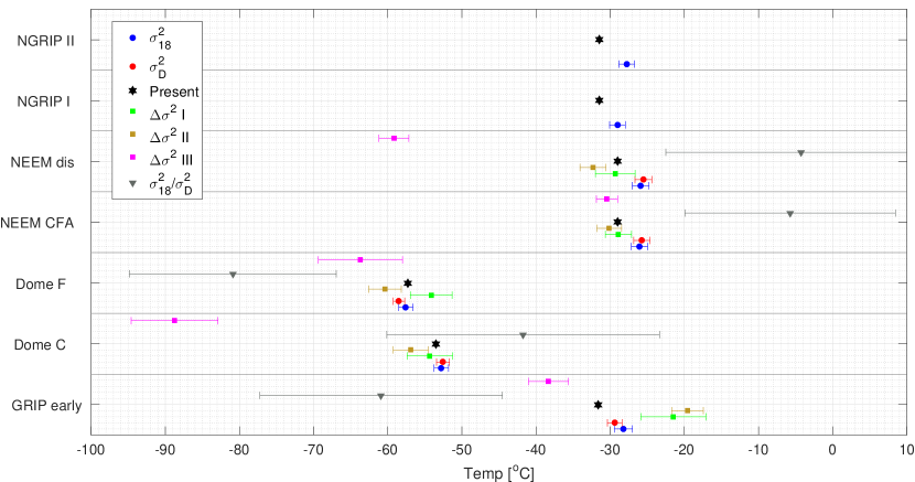
Figure 13: Early Holocene section with reconstructed temperatures from the $\sigma^{2}_{18}$ (blue circles), $\sigma^{2}_{\mathrm{D}}$ (red circles), $\Delta\sigma^{2}$ I (green squares), $\Delta\sigma^{2}$ II (brown squares), $\Delta\sigma^{2}$ III (magenta squares) and ${\sigma^{2}_{18}}/{\sigma^{2}_{\mathrm{D}}}$ (grey triangles) methods. The black stars represent the present annual mean temperatures at the sites.

TABLE IV: Ice core results with the estimated firn diffusion lengths and their corresponding temperatures [^oC]. The units for the $\sigma_{18}$ and the $\sigma_{\mathrm{D}}$ values are expressed in $\mathrm{cm}$ and the unit for ${}^{18}\Delta\sigma^{2}$ is expressed in $\mathrm{cm}^{2}$.

Site Name	$\sigma_{18}$	$\sigma_{\mathrm{D}}$	${}^{18}\Delta\sigma^{2}$ I	${}^{18}\Delta\sigma^{2}$ II	${}^{18}\Delta\sigma^{2}$ III	$\sigma^{2}_{18}/\sigma^{2}_{\mathrm{D}}$
GRIP mid	7.83 $\pm$ 0.17$\,\mathrm{cm}$	7.20 $\pm$ 0.16$\,\mathrm{cm}$	9.4 $\pm$ 1.0$\,\mathrm{cm}^{2}$	9.6 $\pm$ 0.7$\,\mathrm{cm}^{2}$	0.2$\pm$ 0.1$\,\mathrm{cm}^{2}$	1.18$\pm$ 0.02
	-33.0$\pm$ 1.1$\,{}^{\mathrm{o}}$C	-33.0$\pm$ 1.0$\,{}^{\mathrm{o}}$C	-32.7 $\pm$ 2.0$\,{}^{\mathrm{o}}$C	-32.3 $\pm$ 1.5$\,{}^{\mathrm{o}}$C	-80.6 $\pm$ 2.9$\,{}^{\mathrm{o}}$C	-34.4 $\pm$ 6.6$\,{}^{\mathrm{o}}$C
GRIP late	8.52 $\pm$ 0.12$\,\mathrm{cm}$	7.92 $\pm$ 0.16$\,\mathrm{cm}$	9.9 $\pm$ 0.8$\,\mathrm{cm}^{2}$	8.6 $\pm$ 0.5$\,\mathrm{cm}^{2}$	4.8$\pm$ 0.5$\,\mathrm{cm}^{2}$	1.16$\pm$ 0.02
	-30.6 $\pm$ 1.1$\,{}^{\mathrm{o}}$C	-30.5 $\pm$ 1.1$\,{}^{\mathrm{o}}$C	-31.8 $\pm$ 1.8$\,{}^{\mathrm{o}}$C	-34.1 $\pm$ 1.5$\,{}^{\mathrm{o}}$C	-43.0 $\pm$ 1.7$\,{}^{\mathrm{o}}$C	-24.4 $\pm$ 8.7$\,{}^{\mathrm{o}}$C
WAIS 2005A	7.05 $\pm$ 0.11$\,\mathrm{cm}$	————–	————–	————–	————–	————–
	-31.7 $\pm$ 1.1$\,{}^{\mathrm{o}}$C	————–	————–	————–	————–	————–
EDML	7.72 $\pm$ 0.09$\,\mathrm{cm}$	7.12 $\pm$ 0.08$\,\mathrm{cm}$	8.9 $\pm$ 0.3$\,\mathrm{cm}^{2}$	8.1 $\pm$ 0.3$\,\mathrm{cm}^{2}$	7.1$\pm$ 0.2$\,\mathrm{cm}^{2}$	1.18$\pm$ 0.01
	-42.8 $\pm$ 0.9$\,{}^{\mathrm{o}}$C	-42.5 $\pm$ 0.9$\,{}^{\mathrm{o}}$C	-44.6 $\pm$ 1.1$\,{}^{\mathrm{o}}$C	-45.9 $\pm$ 1.0$\,{}^{\mathrm{o}}$C	-47.6 $\pm$ 1.0$\,{}^{\mathrm{o}}$C	-32.4 $\pm$ 3.1$\,{}^{\mathrm{o}}$C
NEEM	7.98 $\pm$ 0.22$\,\mathrm{cm}$	7.20 $\pm$ 0.32$\,\mathrm{cm}$	11.8 $\pm$ 1.6$\,\mathrm{cm}^{2}$	10.2 $\pm$ 1.1$\,\mathrm{cm}^{2}$	4.5$\pm$ 2.0$\,\mathrm{cm}^{2}$	1.23$\pm$ 0.05
	-31.8 $\pm$ 1.1$\,{}^{\mathrm{o}}$C	-32.4 $\pm$ 1.4$\,{}^{\mathrm{o}}$C	-28.4 $\pm$ 2.6$\,{}^{\mathrm{o}}$C	-30.7 $\pm$ 2.1$\,{}^{\mathrm{o}}$C	-45.9 $\pm$ 10.1$\,{}^{\mathrm{o}}$C	-49.3 $\pm$ 15.0$\,{}^{\mathrm{o}}$C
NGRIP	9.24 $\pm$ 0.20 $\mathrm{cm}$	————–	————–	————–	————–	————–
	-29.8 $\pm$ 1.1$\,{}^{\mathrm{o}}$C	————–	————–	————–	————–	————–
Dome F	5.76 $\pm$ 0.15$\,\mathrm{cm}$	4.92 $\pm$ 0.06$\,\mathrm{cm}$	9.0 $\pm$ 1.8$\,\mathrm{cm}^{2}$	5.4 $\pm$ 0.8$\,\mathrm{cm}^{2}$	4.4$\pm$ 1.9$\,\mathrm{cm}^{2}$	1.37$\pm$ 0.08
	-57.6 $\pm$ 1.0$\,{}^{\mathrm{o}}$C	-58.5 $\pm$ 0.8$\,{}^{\mathrm{o}}$C	-54.2 $\pm$ 2.8$\,{}^{\mathrm{o}}$C	-60.4 $\pm$ 2.2$\,{}^{\mathrm{o}}$C	-63.7 $\pm$ 5.7$\,{}^{\mathrm{o}}$C	-80.9 $\pm$ 14.0$\,{}^{\mathrm{o}}$C
Dome C	6.97 $\pm$ 0.15$\,\mathrm{cm}$	6.34 $\pm$ 0.08$\,\mathrm{cm}$	8.4 $\pm$ 1.9$\,\mathrm{cm}^{2}$	6.7 $\pm$ 1.1$\,\mathrm{cm}^{2}$	0.4$\pm$ 0.4$\,\mathrm{cm}^{2}$	1.21$\pm$ 0.05
	-52.8 $\pm$ 1.0$\,{}^{\mathrm{o}}$C	-52.5 $\pm$ 0.9$\,{}^{\mathrm{o}}$C	-54.3 $\pm$ 3.0$\,{}^{\mathrm{o}}$C	-56.9 $\pm$ 2.3$\,{}^{\mathrm{o}}$C	-88.8 $\pm$ 5.9$\,{}^{\mathrm{o}}$C	-42.8 $\pm$ 18.4$\,{}^{\mathrm{o}}$C
GRIP early	9.31 $\pm$ 0.24$\,\mathrm{cm}$	8.25 $\pm$ 0.09$\,\mathrm{cm}$	18.7 $\pm$ 4.0$\,\mathrm{cm}^{2}$	20.4 $\pm$ 1.9$\,\mathrm{cm}^{2}$	6.6$\pm$ 1.1$\,\mathrm{cm}^{2}$	1.27$\pm$ 0.06
	-28.2 $\pm$ 1.2$\,{}^{\mathrm{o}}$C	-29.4 $\pm$ 1.0$\,{}^{\mathrm{o}}$C	-21.5 $\pm$ 4.4$\,{}^{\mathrm{o}}$C	-19.6 $\pm$ 2.1$\,{}^{\mathrm{o}}$C	-38.4 $\pm$ 2.7$\,{}^{\mathrm{o}}$C	-60.9 $\pm$ 16.4$\,{}^{\mathrm{o}}$C
NEEM dis	10.33 $\pm$ 0.19$\,\mathrm{cm}$	9.72 $\pm$ 0.20$\,\mathrm{cm}$	12.1 $\pm$ 1.8$\,\mathrm{cm}^{2}$	10.0 $\pm$ 0.9$\,\mathrm{cm}^{2}$	1.6$\pm$ 0.2$\,\mathrm{cm}^{2}$	1.13$\pm$ 0.02
	-25.9 $\pm$ 1.1$\,{}^{\mathrm{o}}$C	-25.5 $\pm$ 1.1$\,{}^{\mathrm{o}}$C	-29.3 $\pm$ 2.7$\,{}^{\mathrm{o}}$C	-32.3 $\pm$ 1.8$\,{}^{\mathrm{o}}$C	-59.2 $\pm$ 2.0$\,{}^{\mathrm{o}}$C	-4.2 $\pm$ 18.3$\,{}^{\mathrm{o}}$C
NEEM CFA	10.27 $\pm$ 0.19$\,\mathrm{cm}$	9.65 $\pm$ 0.18$\,\mathrm{cm}$	12.3 $\pm$ 1.1$\,\mathrm{cm}^{2}$	11.4 $\pm$ 0.9$\,\mathrm{cm}^{2}$	11.2$\pm$ 0.6$\,\mathrm{cm}^{2}$	1.13$\pm$ 0.01
	-26.1 $\pm$ 1.1$\,{}^{\mathrm{o}}$C	-25.7 $\pm$ 1.1$\,{}^{\mathrm{o}}$C	-29.0 $\pm$ 1.8$\,{}^{\mathrm{o}}$C	-30.1 $\pm$ 1.7$\,{}^{\mathrm{o}}$C	-30.4 $\pm$ 1.4$\,{}^{\mathrm{o}}$C	-5.7 $\pm$ 14.2$\,{}^{\mathrm{o}}$C
NGRIP I	9.68 $\pm$ 0.16$\,\mathrm{cm}$	————–	————–	————–	————–	————–
	-29.0 $\pm$ 1.1$\,{}^{\mathrm{o}}$C	————–	————–	————–	————–	————–
NGRIP II	10.14 $\pm$ 0.17$\,\mathrm{cm}$	————–	————–	————–	————–	————–
	-27.8 $\pm$ 1.0$\,{}^{\mathrm{o}}$C	————–	————–	————–	————–	————–

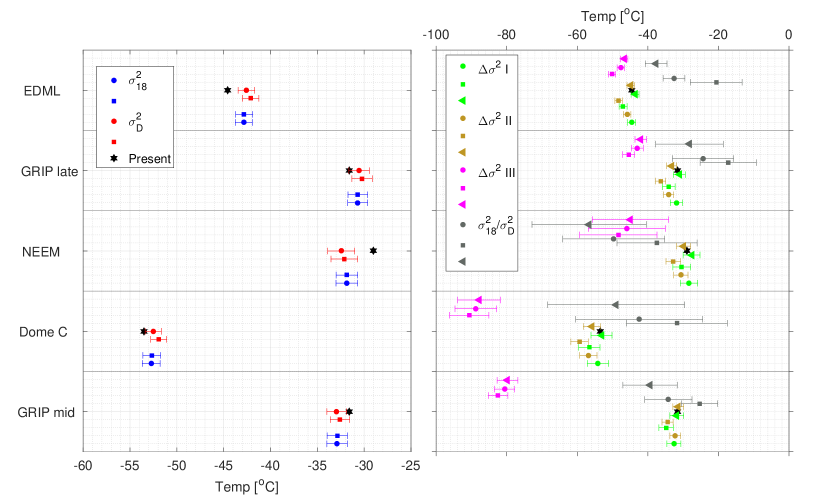
Figure 14: Temperature reconstructions based on different fractionation factor parameterizations. The left figure shows the single isotopologue methods and the right figure shows the dual isotope methods. Circles correspond to fractionation factors from [40, 43], squares correspond to fractionation factors from [18] and triangles from [37, 40].

V Discussion

V-A Synthetic data

Based on the results of the sensitivity experiment with synthetic data, the following can be inferred. Firstly, the three techniques based on the single isotope diffusion, perform similarly and of all the techniques tested, yield the highest precision with a $s_{\bar{T}}\approx 1.0\,{}^{\circ}\text{C}$ (the average precision $s_{\bar{T}}$ of each technique is calculated by averaging the variances of all simulations). Additionally, the estimated temperatures $\overline{T}$ are within 1$s_{\bar{T}}$ of the forcing temperature $T_{\text{sur}}$, a result pointing to a good performance with respect to the accuracy of the temperature estimation.

The precision of the differential diffusion techniques is slightly inferior to single diffusion with the subtraction technique being the least precise of all three differential diffusion approaches ($s_{\bar{T}}\approx 2.6\,{}^{\circ}\text{C}$). A possible reason for this result may be the fact that the subtraction technique relies on the tuning of 8 optimization parameters as described in Sec. III-A and III-B. Both the linear fit and the correlation techniques yield precision estimates of $1.8\,{}^{\circ}\text{C}$ and $1.3\,{}^{\circ}\text{C}$, respectively. Despite the high precision of the correlation technique, the tests shows that the technique has a bias toward colder temperatures. The linear fit is therefore the most optimal of the differential diffusion techniques. All 10 experiments utilizing differential diffusion methods, yield an accuracy that lies within the 2$s_{\bar{T}}$ range (1$s_{\bar{T}}$ range for 9 out of 10 experiments). We can conclude that experiments involving the estimation of the diffusion length ratio indicate that the latter are practically unusable due to very high uncertainties with $s_{\bar{T}}$ averaging to a value of $\approx 16\,{}^{\circ}\text{C}$ for all four experiments. A general trend that seems to be apparent for all the experiments, is that the results for the case A forcing yield slightly lower uncertainties when compared to those for the case B forcing, likely indicating a temperature and accumulation influence in the performance of all the reconstruction techniques.

V-B Ice core data

V-B1 The estimation of diffusion length from spectra

From the spectra presented in SOM Sec. S6, we can see that the diffusion plus noise model (Eq. 11) provides good fits to the ice core data. For ice core sections with a resolution equal to (or higher than) $2.5\,\mathrm{cm}$, we start seeing a difference in the spectral signature of the noise tail between the data from Greenland and Antarctica. The low accumulation Antarctic ice core sites seem to best represent the diffusion plus white noise model used in the synthetic data test. For instance, the PSD of Dome C in Fig. S32 resembles well that of the synthetic data in Fig. 5, whereas a slightly more red noise tail is evident for the high accumulation sites on Greenland. We don’t know why the noise for some of the Greenlandic sites behaves differently, but the white noise of the Antarctic ice core data coincides well with isotopic signals that likely comprise of a few events per year and is whiten due to post depositional effects such as snow relocation. Nonetheless, the AR-1 noise model in Eq. 11 describes both the red and white noise well.

An example of how sample resolution plays a role in assessing the value of the estimated diffusion length, can be seen when visually comparing the spectra of the NEEM early Holocene data in Fig. S8 and S11. The lack of sufficient resolution in Fig S11 (discrete $5\,\mathrm{cm}$ data) results in a poorly resolved noise signal. On the contrary, the $0.5\,\mathrm{cm}$ resolution of the CFA obtained data (both datasets are from approximately the same depth interval) allows for a much better insight into the noise characteristics of the isotopic time series and therefore a more robust diffusion length estimation. Despite differences in the resolution of the power spectra, the fitting procedure provides similar estimates of the firn diffusion lengths as seen in Table IV. This result indicates that even though the diffusion length can be estimated with less certainty, the diffusion length is still preserved in the signal which underlines how powerful a technique the spectral estimation of diffusion length is.

In this study, the annual peak is removed in five out of thirteen cases. However, we do not see any distinguished multiannual variability manifested as spectral peaks. A correction similar to that of the annual peak filter is therefore not implemented. This does not necessarily mean that there is no imprint in those bands to start with, but our analysis does not indicate this and these signals are either too weak to noticeably affect the fits of the assumed model (i.e. diffusion plus noise) or they cannot be resolved at all because their power lies lower than the measurement noise.

V-B2 The temperature reconstructions

The precision $s_{\bar{T}}$ of each reconstruction technique has been quantified by averaging the variances of the reconstructed temperatures (Table IV). In accordance with the results from the synthetic data test, the most precise reconstructions are obtained when using the single isotope diffusion methods. The single diffusion methods have a $s_{\bar{T}}$ of $1.1\,^{\mathrm{o}}\mathrm{C}$, while the differential diffusion methods ${}^{18}\Delta\sigma^{2}$ I, II and III have a $s_{\bar{T}}$ of $2.6\,^{\mathrm{o}}\mathrm{C}$, $1.9\,^{\mathrm{o}}\mathrm{C}$ and $4.8\,^{\mathrm{o}}\mathrm{C}$, respectively. The correlation-based technique is hereby shown to be the least precise differential diffusion method. This differs from the result of the synthetic data, where the correlation-based technique had the most precise results. Of the differential diffusion methods, the linear fit of the logarithmic ratio provides the most precise results, with a precision similar to that found from the synthetic data (Sec. V-A). Of all the tested techniques, the diffusion length ratio method is the least precise with a $s_{\bar{T}}$ of $11.8\,^{\mathrm{o}}\mathrm{C}$. A similar precision was found from the synthetic data.

The perturbations of the model parameters help achieve a realistic view on the overall precision and it facilitates a comparison between the single and the differential diffusion techniques. Nonetheless, we want to emphasize that the presented precisions do not represent the absolute obtainable precision of the diffusion-based temperature reconstruction techniques. While the uncertainties presented in Table I represents typical Holocene values estimated for Central Greenland and the East Antarctic Ice Cap, the input parameters’ uncertainties in the firn diffusion model are essentially both depth and site dependent. For instance, we have a better knowledge about the ice flow thinning at a low accumulation site e.g. Dome C compared to that of a high accumulation site e.g. NGRIP for early Holocene ice core data, This is a result of the Dome C site’s early Holocene period being at a depth of $300\,\mathrm{m}$ while the NGRIP site’s early Holocene period is at a depth of $1300\,\mathrm{m}$. Additionally, it is more more difficult to estimate the glacial accumulation rate at sites where the present day values already are very low. Basically, inferring a change between $3\,\mathrm{cm/yr}$ and $1.5\,\mathrm{cm/yr}$ (and how stable this $1.5\,\mathrm{cm/yr}$ estimate is during the glacial) is much harder and with higher uncertainties compared to going from $23\,\mathrm{cm/yr}$ to $10\,\mathrm{cm/yr}$ (where annual layer thickness information is available from chemistry). Similarly, $\rho_{co}$ and $\rho_{o}$ are better known for Holocene conditions and likely close to present day values while glacial conditions represent a regime at which those values may change more considerably. Thus, when utilizing the diffusion techniques on long ice core records, we propose that the uncertainties of such model parameters and corrections should be based on specific characteristics of the ice core site and the part (or depth) of the core under consideration.

It is not possible to quantify the accuracy of the methods when applied on short ice core data sections, as the reconstructed temperatures represent the integrated firn column temperature. Even though the firn diffusion model has a polythermal firn layer due to the seasonal temperature variation, we can only estimate a single value of the diffusion length from the data (the exact temperature gradients a layer has experienced is unknown). The reconstructed temperatures should therefore not necessarily be completely identical to present day annual temperatures. However, clear outliers can still be inferred from the data as Holocene temperature estimates that deviate with $30\,^{\mathrm{o}}\mathrm{C}$ from the present day annual mean temperatures are unrealistic.

First we address the correlation-based and diffusion length ratio techniques as these two methods result in temperatures that clearly deviate with present day annual mean temperatures (Fig. 12 and 13). Besides the low precision of the diffusion length ratio method, temperature estimates using the the correlation-based and diffusion length ratio techniques are highly inconsistent with the results of the other techniques, with root-mean-square deviations (RMSD) varying from $21\,^{\mathrm{o}}\mathrm{C}$ to $34\,^{\mathrm{o}}\mathrm{C}$. In addition, it can be seen that the correlation-based method results in significantly different temperatures for the discretely and continuously measured NEEM section. A similar difference is not found from the spectral-based methods. Instead, these provide consistent temperatures independent of the processing scheme. The generally poor performance of the correlation-based method on ice core data contradicts the high accuracy and precision of the synthetic reconstructions, and is most likely caused by an oversimplification of the relationship between $\delta\mathrm{D}$ and $\delta^{18}\mathrm{O}$. The generation of the synthetic data is based on the assumption that $\delta\mathrm{D}=8\cdot\delta^{18}\mathrm{O}+10\permil$. However, this premise neglects the time dependent $\mathrm{d_{xs}}$ signal. The correlation-based method can therefore be used to accurately reconstruct synthetic temperatures, while the accuracy and precision are much lower for ice core data, as such data has been influenced by the $\mathrm{d_{xs}}$ signal. In addition, these temperature estimates have been shown to be dependent on the sampling process. The correlation-based method therefore yields uncertain estimates of the differential diffusion length.

The temperature estimates originating from the $\sigma^{2}_{18}$ and $\sigma^{2}_{\mathrm{D}}$ methods are found to have a RMSD of $0.7\,^{\mathrm{o}}\mathrm{C}$. This shows that the $\sigma^{2}_{18}$ and $\sigma^{2}_{\mathrm{D}}$ methods result in similar temperatures, which is consistent with the high accuracies found from the synthetic data test. Furthermore, the early Holocene ice core data from Greenland consistently shows reconstructed temperatures warmer than present day (Fig. 13), which corresponds well with a HCO of around $3\,^{\mathrm{o}}\mathrm{C}$ warming as found by [13, 61]. With the exception of WAIS D, the estimated temperatures for the late-mid Holocene using the $\sigma^{2}_{18}$ and $\sigma^{2}_{\mathrm{D}}$ methods are either slightly warmer or colder than present day (Fig. 12). These sections represent ages ranging from $0.9$ to $3.7$ ka and it is not unreasonable to assume that the sites’ surface temperatures have varied in time. We emphasize that some of the presented ice core sections are as short as $15\,\mathrm{m}$, and that such temperature estimates will potentially be more similar to present day when averaged over a long time series.

The temperature estimates of the ${}^{18}\Delta\sigma^{2}$ I method are similar to the present day annual temperature in six out of nine cases. However, the results of the ${}^{18}\Delta\sigma^{2}$ I and II techniques have a RMSD of $3.8\,^{\mathrm{o}}\mathrm{C}$. The seemingly accurate performance of the ${}^{18}\Delta\sigma^{2}$ I method could be either a coincidence or correct. Two of the similar temperature results are from the NEEM early Holocene data that likely should have had warmer surface temperatures than present day. It is therefore difficult to select the most accurate results as both of the differential diffusion techniques before performed well in the accuracy test with the synthetic data. One should therefore not have a preferred technique without utilizing both methods on longer ice core sections. Basically, the reconstructed temperatures could be similar when the temperatures have been averaged over a longer record. Besides the internal differences in the results of the differential techniques, most of the temperature estimates do not match the results of the single diffusion lengths.

V-C The fractionation factors

The temperature estimates resulting from the different fractionation factor parametrizations are shown in Fig. 14. For each method, the influence of the choice of parametrization on the reconstructed temperatures has been quantified by calculating the RMSD between temperature estimates of two parametrizations. Comparing the parametrizations of [18] to those of [40] and [43], the RMSDs of reconstructions that are based on the single diffusion lengths $\sigma^{2}_{18}$ and $\sigma^{2}_{\mathrm{D}}$ are $0.04^{\mathrm{o}}\mathrm{C}$ and $0.4^{\mathrm{o}}\mathrm{C}$. Thus, it is evident that the choice of fractionation factors has an insignificant effect on the results of the $\sigma^{2}_{18}$ method and a small effect on the results of the $\sigma^{2}_{\mathrm{D}}$ method. The choice of parameterization has a greater effect on the temperatures of the ${}^{18}\Delta\sigma^{2}$ techniques, where the temperature estimate of the ${}^{18}\Delta\sigma^{2}$ I, II and III techniques have RMSDs of $2.3^{\mathrm{o}}\mathrm{C}$, $2.3^{\mathrm{o}}\mathrm{C}$ and $2.2^{\mathrm{o}}\mathrm{C}$, respectively. Comparing the parametrization of [37] to that of [43], the temperatures of the ${}^{18}\Delta\sigma^{2}$ I, II and III techniques have RMSDs of $0.9^{\mathrm{o}}\mathrm{C}$, $0.9^{\mathrm{o}}\mathrm{C}$ and $1.0^{\mathrm{o}}\mathrm{C}$, respectively. In general, smaller RMSDs are found when comparing with temperature estimates based on the [37] parametrization. For instance, comparing the temperatures of the ${\sigma^{2}_{18}}/{\sigma^{2}_{\mathrm{D}}}$ technique based on [37] with those of [43], the ${\sigma^{2}_{18}}/{\sigma^{2}_{\mathrm{D}}}$ technique yields a RMSD of $5.9^{\mathrm{o}}\mathrm{C}$, while the RMSD is $11.0^{\mathrm{o}}\mathrm{C}$ when comparing the results based on the parametrizations of [18] with those of [40] and [43]. There are two reasons to why the RMSDs are smaller when comparing with the [37] parametrization: the parametrized $\alpha_{\mathrm{D}}$ of [43] differs more with that of [18] than with that of [37], and the same $\alpha_{18}$ parametrization is used when comparing with [37].

The ${\sigma^{2}_{18}}/{\sigma^{2}_{\mathrm{D}}}$ method is significantly more influenced by the fractionation factors. The high RMSDs imply that even if the diffusion length ratio is estimated with high confidence, the method is still too sensitive to the choice of parameterization. This makes the method less suitable as a paleoclimatic thermometer.

V-D Outlook with respect to ice core measurements

It is obvious from the analysis we present here that the type of isotopic analysis chosen has an impact on the quality of the power spectral estimates and subsequently on the diffusion length estimation. One such important property of the spectral estimation that is directly dependent on the nature of the isotopic analysis is the achievable Nyquist frequency, defined by the sampling resolution $\Delta$ of the isotopic time series. The value of the Nyquist frequency $f_{\mathrm{Nq}}$ sets the limit in the frequency space until which a power spectral estimate can be obtained. The higher the value of $f_{\mathrm{Nq}}$, the more likely it is that the noise part ${|\hat{\eta}\left(k\right)|}^{2}$ of the power spectrum will be resolved by the spectral estimation routine. The deeper the section under study, the higher the required $f_{\mathrm{Nq}}$ due to the fact that the ice flow thinning results in a progressively lower value for the diffusion length and as a result the diffusion part of the spectrum extents more into the higher frequencies. This effect manifests particularly in the case of the early Holocene Greenland sections of this study. For the case of the NEEM early Holocene record, one can observe the clear benefit of the higher sampling resolution by comparing the discrete ($\Delta=5\;\mathrm{cm}$) to the the CFA ($\Delta=0.5\;\mathrm{cm}$) data set. Characterizing the noise signal ${|\hat{\eta}\left(k\right)|}^{2}$ is more straight forward in the case of the CFA data. On the contrary, at these depths of the NEEM core, the resolution of $5\;\mathrm{cm}$ results in the spectral estimation not being able to resolve the noise signal.

The diffusion of the sampling and measurement process itself is a parameter that needs to be thoroughly addressed particularly during the development and construction of a CFA system as well as during the measurement of an ice core with such a system. Ideally, one would aim for (a) a dispersive behavior that resembles as close as possible that of Gaussian mixing, (b) a measurement system diffusion length $\sigma_{\mathrm{cfa}}$ that is as low as possible and (c) a diffusive behavior that is stable as a function of time. Real measurements with CFA systems indicate that most likely due to surface effects in the experimental apparatus that lead to sample memory, the transfer functions of such systems depart from the ideal model of Gaussian dispersion showing a slightly skewed behavior. For some systems, this behavior resembles more that of a slightly skewed Log-Normal distribution [23, 41, 19] or a more skewed distribution that in the case of [32] requires the product of two Log-Normal distributions to be accurately modeled. The result of this behavior to the power spectral density is still a matter of further study as high resolution datasets obtained with CFA systems are relatively recent.

Additionally the accuracy of the depth registration is essential in order for accurate spectral estimates to be possible. Instabilities in melt rates of the ice stick under consideration can in principle be addressed and a first-order correction can be available assuming a length encoder is installed in the system. Such a correction though does not take into account the fact that due to the constant sample flow rate through the CFA system, the constant mixing volume of the system’s components (sample tubing, valves etc) will cause a variable mixing as melt rates change. The magnitudes and importance of these variations are not easy to assess and more work will be required in the future in order to characterize and correct for these effects.

Due to the recent advances in laser spectroscopy we expect measurements of the $\delta^{17}$O signal to be a common output from analyzed ice cores. As we showed with synthetic data, such a signal can also be used to reconstruct temperatures. Especially the differential diffusion length of $\delta^{17}$O and $\delta$D showed higher precision than that of $\delta^{18}$O and $\delta$D. Such measurements however, require that laboratories around the world have access to well calibrated standards. Calibration protocols for $\delta^{17}$O have been suggested [51] although there is still a lack of $\delta^{17}$O values for the International Atomic Energy Agency standards VSMOW (Vienna Standard Mean Ocean Water) and SLAP (Standard Light Antarctic Precipitation).

VI Conclusions

This study assessed the performance of six different diffusion-based temperature reconstruction techniques. By applying the methods on synthetic data, first order tests of accuracy and bias were demonstrated and evaluated. Moreover, this approach facilitated precision estimates of each method. The precision of each technique was further quantified by utilizing every variety of the diffusion-based temperature proxy on thirteen high resolution data sets from Greenland and Antarctica. The results showed that the single diffusion length methods yielded similar temperatures and that they are the most precise of all the presented reconstruction techniques. The most precise of the three differential diffusion length techniques was the linear fit of the logarithmic ratio. The most uncertain way of reconstructing past temperatures was by employing the diffusion length ratio method. The results from the correlation-based method were inconsistent to the results obtained through the spectral-based methods, and the method was considered to yield uncertain estimates of the differential diffusion length.

It was furthermore shown that the choice of fractionation factor parametrization only had a small impact on the results from the single diffusion length methods, while the influence was slightly higher for the differential diffusion length methods. The diffusion length ratio method was highly sensitive to the fractionation factor parametrization, and the method is not suitable as a paleoclimatic thermometer.

In conclusion, despite that the dual diffusion techniques seem to be the more optimal choices due to their independence of sampling and ice diffusion or densification and thinning processes, the uncertain estimates should outweigh the theoretical advantages for Holocene ice core data.

References

- [1] Milton Abramowitz and Irene A. Stegun. Handbook of Mathematical Functions with Formulas, Graphs, and Mathematical Tables. Dover, 9th edition, 1964.
- [2] N. Andersen. On The Calculation Of Filter Coefficients For Maximum Entropy Spectral Analysis. Geophysics, 39(1), 1974.
- [3] L. Baker, I. A. Franchi, J. Maynard, I. P. Wright, and C. T. Pillinger. A technique for the determination of O-18/O-16 and O-17/O-16 isotopic ratios in water from small liquid and solid samples. Analytical Chemistry, 74(7):1665–1673, 2002.
- [4] J. R. Banta, J. R. McConnell, M. M. Frey, R. C. Bales, and K. Taylor. Spatial and temporal variability in snow accumulation at the West Antarctic Ice Sheet Divide over recent centuries. Journal of Geophysical Research, 113, 2008.
- [5] E. Barkan and B. Luz. High precision measurements of O-17/O-16 and O-18/O-16 ratios in (H2O). Rapid Communications In Mass Spectrometry, 19(24):3737–3742, 2005.
- [6] I. S. Begley and C. M. Scrimgeour. High-precision and measurement for water and volatile organic compounds by continuous-flow pyrolysis isotope ratio mass spectrometry. Analytical Chemistry, 69(8):1530–1535, 1997.
- [7] J. Bigeleisen, M. L. Perlman, and H. C. Prosser. Conversion of hydrogenic materials to hydrogen for isotopic analysis. Analytical Chemistry, 24(8):1356–1357, 1952.
- [8] H. Blicks, O. Dengel, and N. Riehl. Diffusion von protonen (tritonen) in reinen und dotierten eis-einkristallen. Physik Der Kondensiterten Materie, 4(5):375–381, 1966.
- [9] W. A. Brand, Heike Geilmann, Eric R. Crosson, and Chris W. Rella. Cavity ring-down spectroscopy versus high-temperature conversion isotope ratio mass spectrometry; a case study on and of pure water samples and alcohol/water mixtures. Rapid Communications in Mass Spectrometry, 23(12):1879–1884, 2009.
- [10] H. Craig. Isotopic Variations in Meteroric Water. Science, 133(3465):1702–1703, 1961.
- [11] E. R. Crosson. A cavity ring-down analyzer for measuring atmospheric levels of methane, carbon dioxide, and water vapor. Applied Physics B-Lasers And Optics, 92(3):403–408, 2008.
- [12] K. M. Cuffey, R. B. Alley, P. M. Grootes, J. M. Bolzan, and S. Anandakrishnan. Calibration Of the Delta-O-18 isotopic paleothermometer for central Greenland, using borehole temperatures. Journal Of Glaciology, 40(135):341–349, 1994.
- [13] D. Dahl-Jensen, K. Mosegaard, N. Gundestrup, G. D Clow, S. J. Johnsen, A. W. Hansen, and N. Balling. Past temperatures directly from the Greenland Ice Sheet. Science, 282(5387):268–271, 1998.
- [14] W. Dansgaard. The 18O-abundance in fresh water. Geochimica et Cosmochimica Acta, 6(5–6):241–260, 1954.
- [15] W. Dansgaard. Stable isotopes in precipitation. Tellus B, 16(4):436–468, 1964.
- [16] W. Dansgaard and S. J. Johnsen. A flow model and a time scale for the ice core from Camp Century, Greenland. Journal of Glaciology, 8(53), 1969.
- [17] P. Delibaltas, O. Dengel, D. Helmreich, N. Riehl, and H. Simon. Diffusion von in eis-einkristallen. Physik Der Kondensiterten Materie, 5(3):166–170, 1966.
- [18] M. D. Ellehoj, H. C. Steen-Larsen, S. J. Johnsen, and M. B. Madsen. Ice-vapor equilibrium fractionation factor of hydrogen and oxygen isotopes: Experimental investigations and implications for stable water isotope studies. Rapid Communications in Mass Spectrometry, 27:2149–2158, 2013.
- [19] B. D. Emanuelsson, W. T. Baisden, N. A. N. Bertler, E. D. Keller, and V. Gkinis. High-resolution continuous-flow analysis setup for water isotopic measurement from ice cores using laser spectroscopy. Atmos. Meas. Tech., 8(7):2869–2883, 2015.
- [20] S. Epstein, R. Buchsbaum, H. Lowenstam, and H.C. Urey. Carbonate-water isotopic temperature scale. Geological Society of America Bulletin, 62(4):417, 1951.
- [21] M. Gehre, R. Hoefling, P. Kowski, and G. Strauch. Sample preparation device for quantitative hydrogen isotope analysis using chromium metal. Analytical Chemistry, 68(24):4414–4417, 1996.
- [22] V. Gkinis. High resolution water isotope data from ice cores. PhD thesis, University of Copenhagen, 2011.
- [23] V. Gkinis, T. J. Popp, T. Blunier, M. Bigler, S. Schupbach, E. Kettner, and S. J. Johnsen. Water isotopic ratios from a continuously melted ice core sample. Atmospheric Measurement Techniques, 4(11):2531–2542, 2011.
- [24] V. Gkinis, S. B. Simonsen, S. L. Buchardt, J. W. C. White, and B. M. Vinther. Water isotope diffusion rates from the NorthGRIP ice core for the last 16,000 years - glaciological and paleoclimatic implications. Earth and Planetary Science Letters, 405, 2014.
- [25] M. Guillevic, L. Bazin, A. Landais, P. Kindler, A. Orsi, V. Masson-Delmotte, T. Blunier, S. L. Buchardt, E. Capron, M . Leuenberger, P. Martinerie, F. Prie, and B. M. Vinther. Spatial gradients of temperature, accumulation and O-ice in Greenland over a series of Dansgaard–-Oeschger events. Climate of the Past, 9:1029–1051, 2013.
- [26] Kazuhiko Itagaki. Self-diffusion in single crystals of ice. J. Phys. Soc. Jpn., 19(6):1081–1081, 1964.
- [27] S. J. Johnsen. Stable Isotope Homogenization of Polar Firn and Ice. Isotopes and Impurities in Snow and Ice, pages 210–219, 1977.
- [28] S. J. Johnsen, D. Dahl Jensen, W. Dansgaard, and N. Gundestrup. Greenland paleotemperatures derived from GRIP bore hole temperature and ice core isotope profiles. Tellus B-Chemical And Physical Meteorology, 47(5):624–629, 1995.
- [29] S. J. Johnsen, D. Dahl-Jensen, N. Gundestrup, J. P. Steffensen, H. B. Clausen, H. Miller, V. Masson-Delmotte, A. E. Sveinbjörnsdottir, and J. White. Oxygen isotope and palaeotemperature records from six Greenland ice-core stations: Camp Century, Dye-3, GRIP, GISP2, Renland and NorthGRIP. Journal of Quaternary Science, 16(4), 2001.
- [30] S. J. Johnsen and J. White. The origin of Arctic precipitation under present and glacial conditions. Tellus, 41B:452–468, 1989.
- [31] S.J. Johnsen, H. B. Clausen, K. M. Cuffey, G. Hoffmann, J. Schwander, and T. Creyts. Diffusion of stable isotopes in polar firn and ice: the isotope effect in firn diffusion. Physics of Ice Core Records, pages 121–140, 2000.
- [32] T. R Jones, J. W. C. White, E. J. Steig, B. H. Vaughn, V. Morris, V. Gkinis, B. R. Markle, and S. W. Schoenemann. Improved methodologies for continuous-flow analysis of stable water isotopes in ice cores. Atmos. Meas. Tech, 10:617–632, 2017.
- [33] J. Jouzel, R. B. Alley, K. M. Cuffey, W. Dansgaard, P. Grootes, G. Hoffmann, S. J. Johnsen, R. D. Koster, D. Peel, C. A. Shuman, M. Stievenard, M. Stuiver, and J. White. Validity of the temperature reconstruction from water isotopes in ice cores. Journal Of Geophysical Research-Oceans, 102(C12):26471–26487, 1997.
- [34] J. Jouzel and L. Merlivat. Deuterium and oxygen 18 in precipitation: modeling of the isotopic effects during snow formation. Journal of Geophysical Research-Atmospheres, 89(D7):11749 – 11759, 1984.
- [35] K. Kawamura, T. Nakazawa, S. Aoki, S. Sugawara, Y. Fujii, and O. Watanabe. Atmospheric variations over the last three glacial-interglacial climatic cycles deduced from the Dome Fuji deep ice core, Antarctica using a wet extraction technique. Tellus, 55B:126–137, 2003.
- [36] S. M. Kay and S. L. Marple. Spectrum Analysis - A Modern Perspective. Proceedings of the IEEE, 69(11), 1981.
- [37] Kara D. Lamb, Benjamin W. Clouser, Maximilien Bolot, Laszlo Sarkozy, Volker Ebert, Harald Saathoff, Ottmar Möhler, and Elisabeth J. Moyer. Laboratory measurements of HDO/H2O isotopic fractionation during ice deposition in simulated cirrus clouds. PNAS, 114(L22):5612–5617, 2017.
- [38] F. E. Livingston, G. C. Whipple, and S. M. George. Diffusion of HDO into single-crystal (H2O)-O-16 ice multilayers: Comparison with (H2O)-O-18. Journal of Physical Chemistry B, 101(32):6127–6131, 1997.
- [39] C. Lorius, L. Merlivat, J. Jouzel, and M. Pourchet. A 30,000-yr isotope climatic record from Antarctic ice. Nature, 280:644 – 648, 1979.
- [40] M. Majoube. Fractionation factor of 18O between water vapour and ice. Nature, 226(1242), 1970.
- [41] Olivia J. Maselli, Diedrich Fritzsche, Lawrence Layman, Joseph R. McConnell, and Hanno Meyer. Comparison of water isotope-ratio determinations using two cavity ring-down instruments and classical mass spectrometry in continuous ice-core analysis. Isotopes in Environmental and Health Studies, pages 1–12, May 2013.
- [42] H. A. J. Meijer and W. J. Li. The use of electrolysis for accurate delta O-17 and delta O-18 isotope measurements in water. Isotopes In Environmental And Health Studies, 34(4):349–369, 1998.
- [43] L. Merlivat and G. Nief. Fractionnement Isotopique Lors Des Changements Detat Solide-Vapeur Et Liquide-Vapeur De Leau A Des Temperatures Inferieures A 0 Degrees C. Tellus, 19(1):122–127, 1967.
- [44] J. Mook. Environmental Isotopes in the Hydrological Cycle Principles and Applications. International Atomic Energy Agency, 2000.
- [45] NGRIP members. High-resolution record of Northern Hemisphere climate extending into the last interglacial period. Nature, 431(7005):147–151, 2004.
- [46] H. Oerter, W. Graf, H. Meyer, and F. Wilhelms. The EPICA ice core Droning Maud Land: first results from stable-isotope measurements. Ann. Glaciol., 39:307–312, 2004.
- [47] William H. Press, Saul A. Teukolsky, William T. Vetterling, and Brian P. Flannery. Numerical Recipes: The Art of Scientific Computing. Cambridge University Press, August 2007.
- [48] R. O. Ramseier. Self-diffusion of tritium in natural and synthetic ice monocrystals. Journal Of Applied Physics, 38(6):2553–2556, 1967.
- [49] S. O. Rasmussen, P. M. Abbott, T. Blunier, A.J. Bourne, E. Brook, S. L. Buchardt, C. Buizert, J. Chappellaz, H. B. Clausen, E. Cook, D. Dahl-Jensen, S. M. Davies, M. Guillevic, S. Kipfstuhl, T. Laepple, I. K. Seierstad, J.P. Severinghaus, J. P. Steffensen, C. Stowasser, A. Svensson, P. Vallelonga, B. M. Vinther, F. Wilhelms, and M. Winstrup. A first chronology for the North Greenland Eemian Ice Drilling (NEEM) ice core. Climate of the Past, 9:2713–2730, 2013.
- [50] Sune O. Rasmussen, Matthias Bigler, Simon P. Blockley, Thomas Blunier, Susanne L. Buchardt, Henrik B. Clausen, Ivana Cvijanovic, Dorthe Dahl-Jensen, Sigfus J. Johnsen, Hubertus Fischer, Vasileios Gkinis, Myriam Guillevic, Wim Z. Hoek, J. John Lowe, Joel B. Pedro, Trevor Popp, Inger K. Seierstad, Jorgen Pederrgen Peder Steffensen, Anders M. Svensson, Paul Vallelonga, Bo M. Vinther, Mike J.C. Walker, Joe J. Wheatley, and Mai Winstrup. A stratigraphic framework for abrupt climatic changes during the last glacial period based on three synchronized greenland ice-core records: refining and extending the intimate event stratigraphy. Quaternary Science Reviews, 106:14–28, 2014.
- [51] S. W. Schoenemann, A. J. Schauer, and E. J. Steig. Measurement of SLAP2 and GISP O and proposed VSMOW-SLAP normalization for O and . Rapid Commun. Mass Spectrom., 27:582–590, 2013.
- [52] J. P. Severinghaus and E. J. Brook. Abrupt climate change at the end of the last glacial period inferred from trapped air in polar ice. Science, 286(5441):930–934, 1999.
- [53] J. P. Severinghaus, T. Sowers, E. J. Brook, R. B. Alley, and M. L. Bender. Timing of abrupt climate change at the end of the Younger Dryas interval from thermally fractionated gases in polar ice. Nature, 391(6663):141–146, 1998.
- [54] S. B. Simonsen, S. J. Johnsen, T. J. Popp, B. M. Vinther, V. Gkinis, and H. C. Steen-Larsen. Past surface temperatures at the NorthGRIP drill site from the difference in firn diffusion of water isotopes. Climate of the Past, 7, 2011.
- [55] E. J Steig, Q. Ding, J. W. C. White, M. Küttel, S. B. Rupper, T. A. Neumann, P. D. Neff, A. J. E. Gallant, P. A. Mayewski, K. C. Taylor, G. Hoffmann, D. A. Dixon, S. Schoenemann, Markle B. M., D. P. Schneider, T. J Fudge, A. J. Schauer, R. P. Teel, B. Vaughn, L Burgener, J. Williams, and E. Korotkikh. Recent climate and ice-sheet change in West Antarctica compared to the past 2000 years. Nature Geoscience, 6, 2013.
- [56] E. J. Steig, V. Gkinis, A. J. Schauer, S. W. Schoenemann, K. Samek, J. Hoffnagle, K. J. Dennis, and S. M. Tan. Calibrated high-precision 17O-excess measurements using cavity ring-down spectroscopy with laser-current-tuned cavity resonance. Atmos. Meas. Tech., 7(8):2421–2435, 2014.
- [57] A. Svensson, S. Fujita, M. Bigler, M. Braun, R. Dallmayr, V. Gkinis, K. Goto-Azuma, M. Hirabayashi, K. Kawamura, S. Kipfstuhl, H. A. Kjær, T. Popp, M. Simonsen, J. P. Steffensen, P. Vallelonga, and B. M. Vinther. On the occurrence of annual layers in Dome Fuji ice core early Holocene Ice. Climate of the Past, 11:1127–1137, 2015.
- [58] G. van der Wel, H. Fischer, H. Oerter, H. Meyer, and H. A. J. Meijer. Estimation and calibration of the water isotope differential diffusion length in ice core records. The Cryosphere, 9(4):1601–1616, 2015.
- [59] B. H. Vaughn, J. W. C. White, M. Delmotte, M. Trolier, O. Cattani, and M. Stievenard. An automated system for hydrogen isotope analysis of water. Chemical Geology, 152(3-4):309–319, 1998.
- [60] D. Veres, L. Bazin, A. Landais, H. Toye Mahamadou Kele, B. B. Lemieux-Dudon, F. Parrenin, P. Martinerie, E. Blayo, T. Blunier, E. Capron, J. Chappellaz, S. O. Rasmussen, M. Severi, A. Svensson, B. Vinther, and E. W. Wolff. The Antarctic ice core chronology (AICC2012): an optimized multi-parameter and multi-site dating approach for the last 120 thousand years. Climate of the Past, 9, 2013.
- [61] B. M. Vinther, S. L. Buchardt, H. B. Clausen, D. Dahl-Jensen, S. J. Johnsen, D. A. Fisher, R. M. Koerner, D. Raynaud, V. Lipenkov, K. K. Andersen, T. Blunier, S. O. Rasmussen, J. P. Steffensen, and A. M. Svensson. Holocene thinning of the Greenland ice sheet. Nature, 461, 2009.
- [62] B. M. Vinther, H. B. Clausen, S. J. Johnsen, S. O. Rasmussen, K. K. Andersen, S. L. Buchardt, D. Dahl-Jensen, I. K. Seierstad, M. L. Siggaard-Andersen, J. P. Steffensen, A. Svensson, J. Olsen, and J. Heinemeier. A synchronized dating of three greenland ice cores throughout the holocene. Journal Of Geophysical Research-Atmospheres, 111(D13102), 2006.
- [63] O. Watanabe, H. Shoji, Motoyama H. Satow, K and, Y. Fujii, H. Narita, and Aoki S. Dating of the Dome Fuji, Antarctica deep ice core. Mem. Natl Inst. Polar Res., Spec. Issue, 57:25–37, 2003.
- [64] I. M. Whillans and P. M. Grootes. Isotopic diffusion in cold snow and firn. Journal of Geophysical Research - Atmospheres, 90:3910–3918, 1985.