Driven Hofstadter Butterflies and Related Topological Invariants

Abstract

The properties of the Hofstadter butterfly, a fractal, self similar spectrum of a two dimensional electron gas, are studied in the case where the system is additionally illuminated with monochromatic light. This is accomplished by applying Floquet theory to a tight binding model on the honeycomb lattice subjected to a perpendicular magnetic field and either linearly or circularly polarized light. It is shown how the deformation of the fractal structure of the spectrum depends on intensity and polarization. Thereby, the topological properties of the Hofstadter butterfly in presence of the oscillating electric field are investigated. A thorough numerical analysis of not only the Chern numbers but also the $W_{3}$-invariants gives the appropriate insight into the topology of this driven system. This includes a comparison of a direct $W_{3}$-calculation to the method based on summing up Chern numbers of the truncated Floquet Hamiltonian.

I Introduction

The integer quantum Hall effect Klitzing et al. (1980); von Klitzing (1986) marks, in hindsight, the inception of the field of topological insulators Hasan and Kane (2010); Qi and Zhang (2011). This discovery was preceded by a few years by Hofstadter’s seminal work on hopping models on a two-dimensional square lattice in a perpendicular magnetic field Hofstadter (1976). The celebrated Hofstadter butterfly contains the Landau level structure underlying the quantum Hall effect in the limit of small fluxes per unit cell. The relation of the band structure to the Hall conductance at general flux was clarified shortly later Thouless et al. (1982) in terms of Chern numbers Fukui et al. (2005).

Moreover, an important recent direction of work in the area of topological insulators are systems under external driving, mainly by electromagnetic radiation, and the formation of nontrivial topological phases dubbed Floquet topological insulators Oka and Aoki (2009); Kitagawa et al. (2010); Lindner et al. (2011); Gu et al. (2011); Cayssol et al. (2013); Rudner et al. (2013); Mikami et al. (2016); Holthaus (2016); Klinovaja et al. (2016). In fact, the study of light-matter interaction is one of the fastest growing research areas in physics. Here, two-dimensional systems with underlying honeycomb lattice structure have attracted particular interest including graphene Oka and Aoki (2009); Karch et al. (2010); Calvo et al. (2011); Zhou and Wu (2011); Gu et al. (2011); Scholz et al. (2013); Usaj et al. (2014); M.A. Sentef et al. (2015); López et al. (2015a); Wang and Li (2016), silicene López et al. (2015b); Mohan et al. (2016), germanene Mohan et al. (2016); M. Tahir et al. (2016), and transition metal dichalcogenides M. Claassen et al. (2016). To access e.g. in graphene the feasibility of ac-driven fields to generate a finite spin polarization of carriers the effect of periodically driven spin-orbit coupling was studied in Refs. López et al., 2012; A. López et al., 2013.

Furthermore, as seen from the quantum Hall effect von Klitzing (1986), the topological properties of two-dimensional systems are also drastically altered by applying a perpendicular magnetic field also leading to fractal structures as the Hofstadter butterfly Hofstadter (1976); R. Rammal (1985); Hasegawa and Kohmoto (2006); Wang and Gong (2009); Rhim and Park (2012); Yilmaz et al. (2015); Yilmaz and Oktel (2017); Asbóth and Alberti (2017). The question arises in which way an external periodic driving can modify or destroy the fractal structure. Moreover, following the seminal paper by Rudner et al., Ref. Rudner et al., 2013, it becomes clear that the topology analysis of driven systems needs a different approach compared to the static case which goes beyond the Chern number calculation. We are going to address these problems in the present paper.

Concerning the experimental realizability of the theory developed in this paper we first emphasize the pioneering work of measuring the Hofstadter butterfly in m$\acute{\mathrm{o}}$ire superlattices Dean et al. (2013) showing the possibility of measuring the Hofstadter butterfly as well on a hexagonal lattice structure. Utilizing superlattice structures the necessary magnetic field can be lowered to easily accessible field strengths of about tens of Tesla. Furthermore, the formation of Floquet bands exist not only on paper. Using ARPES methods the periodic band structure was resolved in momentum space and even the gap opening of driven topological insulators was realized and measuredWang et al. (2013). Thus, the path to experimental accessibility is already paved by modern techniques and the study presented in this paper aims at giving a better understanding of the fundamental building blocks by focusing on a single graphene sheet subjected to a strong perpendicular magnetic field and externally driven by polarized light.

This paper is organized as follows. First, we treat in section II the Hofstadter butterfly problem Hofstadter (1976) on the honeycomb lattice R. Rammal (1985); Hasegawa and Kohmoto (2006); Yilmaz et al. (2015); Owerre (2018) in a rigorous manner. Then we generalize it in section III to the case with periodic driving, realized by linearly and circularly polarized light. We show some representative numerical results for different frequencies, intensities and polarizations. Finally, the topological properties of the Floquet-Hofstadter problem are characterized with Chern numbers and $W_{3}$-invariants in section IV. Thereby we compare this invariant with the often used summation over Chern numbers in the truncated Floquet space for different frequencies and intensities. We combine an analytical as well as a numerical approach to the above quantities, and close with a summary in section V.

Shortly after a previous version of this work other works on the same subject appeared which stress the role of different regimes of the driving frequency Kooi et al. (2018) and other lattice types Du et al. (2018).

II Hofstadter butterfly for the honeycomb lattice

II.1 Derivation of the Hamiltonian

To model graphene we use a tight-binding model where only nearest neighbor hopping can take place. We choose the lattice vectors as

$$\vec{b}_{1}=a\begin{pmatrix}0\\ \sqrt{3}\end{pmatrix}\quad,\quad\vec{b}_{2}=a\begin{pmatrix}\frac{3}{2}\\ \frac{\sqrt{3}}{2}\end{pmatrix}$$ (1)

with $a$ being the distance between the carbon atoms. The nearest neighbor vectors are

$$\vec{a}_{1}=a\begin{pmatrix}1\\ 0\end{pmatrix}\ ,\ \vec{a}_{2}=\frac{a}{2}\begin{pmatrix}-1\\ \sqrt{3}\end{pmatrix}\ ,\ \vec{a}_{3}=\frac{a}{2}\begin{pmatrix}-1\\ -\sqrt{3}\end{pmatrix}$$ (2)

as depicted in Fig. 1. The position of an arbitrary unit cell is

$$\vec{R}(m,n)=m\vec{b}_{1}+n\vec{b}_{2},\quad m,n\in\mathbb{Z}\;.$$ (3)

In presence of a vector potential the hopping parameter $t$ gets modified by the Peierls phase,

$$t\mapsto t_{m,n}e^{i\phi_{m,n}^{(j)}}\,,$$ (4)

where the phase is the integral over the vector potential along the hopping path

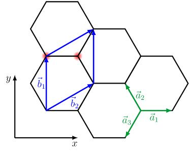
Figure 1: Coordinate geometry used on the honeycomb lattice: The green arrows represent the different nearest neighbor vectors $\vec{a}_{i}$ and the blue ones the lattice vectors $\vec{b}_{i}$.

$$\phi_{m,n}^{(j)}=\frac{e}{\hbar}\int\limits_{\vec{R}(m,n)}^{\vec{R}(m,n)+\vec{a}_{j}}\vec{A}(\vec{r}\,)\cdot\mathrm{d}\vec{r}\;,\quad j=1,2,3\ .$$ (5)

The magnetic field is applied in $z$ direction, $\vec{B}=B\vec{e}_{z}$. For Landau gauge $\vec{A}(\vec{r}\,)=(0,Bx,0)^{T}$ the Peierls phase becomes independent of the index $m$,

$$\int\limits_{\vec{R}(m,n)}^{\vec{R}(m,n)+\vec{a}_{2,3}}\vec{A}(\vec{r}\,)\cdot\mathrm{d}\vec{r}=\pm\frac{3\sqrt{3}}{4}Ba^{2}\bigl{(}n-\tfrac{1}{6}\bigr{)}$$ (6)

and zero for the hopping in $\vec{a}_{1}$ direction. Note that the prefactor in the above expression is related to the area of the elementary unit cell $A_{\mathrm{cell}}$ by $3\sqrt{3}a^{2}/4=A_{\mathrm{cell}}/2$. As usual, we restrict the flux per unit cell in units of the elementary charge over Planck’s constant to a rational value

$$\phi\equiv\frac{e}{h}\,BA_{\mathrm{cell}}=\frac{p}{q}\,.$$ (7)

Thus, the Peierls phase can be written as

$$\frac{e}{\hbar}\frac{3\sqrt{3}}{4}Ba^{2}\bigl{(}n-\tfrac{1}{6}\bigr{)}=\pi\phi\bigl{(}n-\tfrac{1}{6}\bigr{)}$$ (8)

which leads then to the explicit form of of the Hamiltonian

$$\begin{aligned} H=-t\sum_{mn}\Bigl{[}&a^{\dagger}_{m,n}\bigl{(}b_{m,n}+e^{i\pi\phi(n-\frac{1}{6})}b_{m+1,n-1}\\ &+e^{-i\pi\phi(n-\frac{1}{6})}b_{m,n-1}\bigr{)}+\text{h.c.}\Bigr{]}\;,\end{aligned}$$ (9)

where the sum is over all unit cell positions. The solutions of the stationary Schrödinger equation are plane-wave type states of the general form

$$\begin{aligned} |\vec{k}\rangle=\sum_{mn}&e^{i\vec{k}\cdot\vec{R}(m,n)}\bigl{(}\alpha_{n}a_{m,n}^{\dagger}+\beta_{n}b_{m,n}^{\dagger}\bigr{)}|0\rangle\;,\end{aligned}$$ (10)

where the creation operators $a^{\dagger}_{m,n},b^{\dagger}_{m,n}$ for the different sublattice sites are acting on the fermionic vacuum $|0\rangle$. $\alpha_{n},\beta_{n}$ are complex amplitudes depending only on $n$ since the Peierls phase does so, see Eq. (8). Making a projection on a state $\langle 0|a_{m^{\prime},n^{\prime}}$ or $\langle 0|b_{m^{\prime},n^{\prime}}$ leads to a system of coupled equations for the amplitudes

$$-\frac{\varepsilon}{t}\alpha_{n} =\beta_{n}+z_{n}(\vec{k})\beta_{n-1}\;,$$ (11)

$$-\frac{\varepsilon}{t}\beta_{n} =\alpha_{n}+z^{*}_{n+1}(\vec{k})\alpha_{n+1}\;,$$ (12)

with

$$z_{n}(\vec{k})=e^{-i\pi\phi(n-\frac{1}{6})-i\vec{k}\cdot\vec{b_{2}}}+e^{i\pi\phi(n-\frac{1}{6})}e^{i\vec{k}\cdot(\vec{b}_{1}-\vec{b}_{2})}\ .$$ (13)

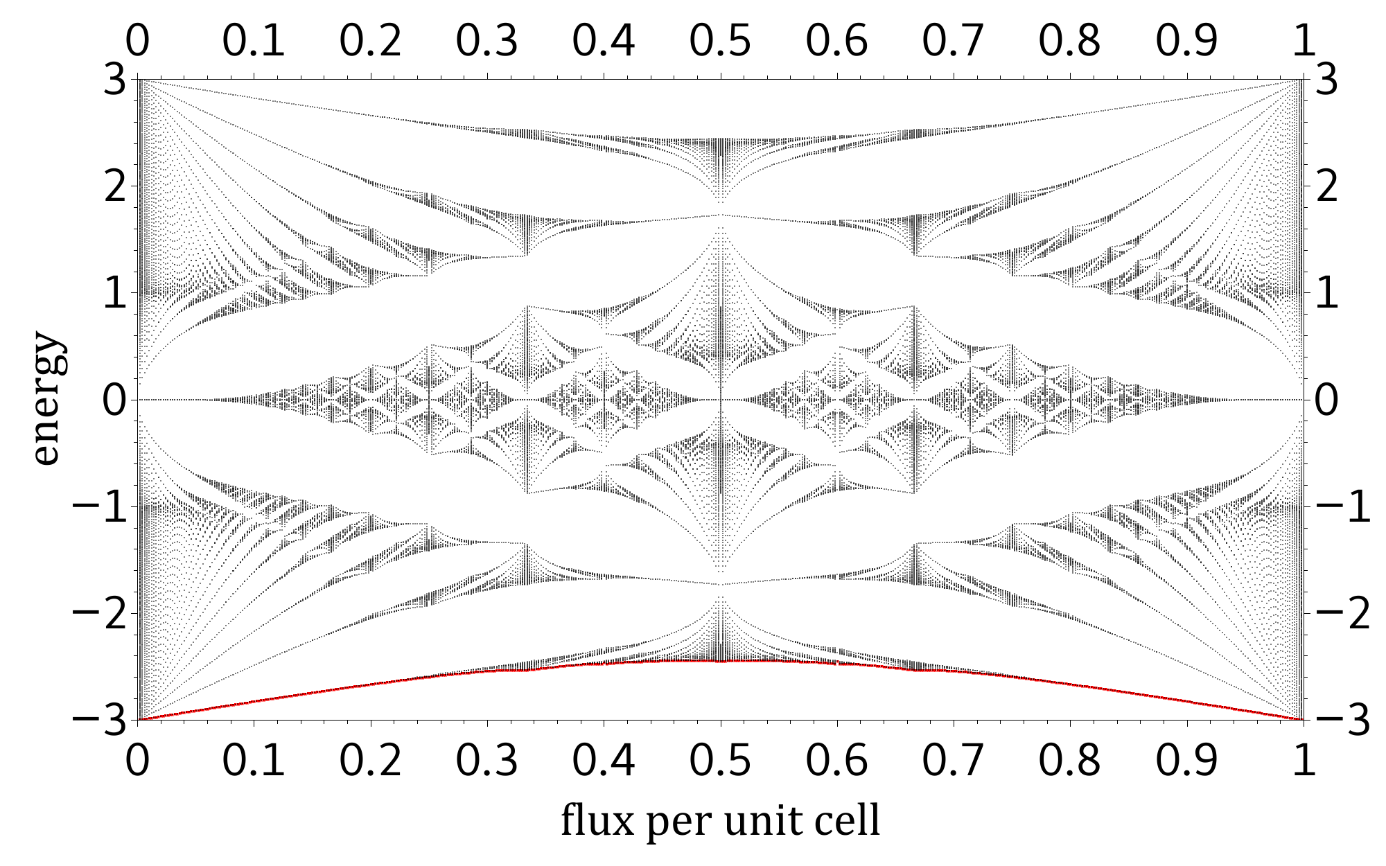
Figure 2: Hofstadter butterfly for the honeycomb lattice. The energy is given in units of the hopping parameter $t$.The ground state of the Hofstadter spectrum is defined as the state with lowest energy represented by the red line.

II.2 Periodicity of the Hofstadter Problem

The Eqs. (11), (12) define a prima vista infinite system of linear equation, which, however, closes to a finite one due to periodicity properties of the amplitudes involved. First, we define the operators

$$T_{r}\begin{pmatrix}a_{m,n}\\ b_{m,n}\end{pmatrix}T^{\dagger}_{r}=\begin{pmatrix}a_{m,n+r}\\ b_{m,n+r}\end{pmatrix}$$ (14)

$$u\begin{pmatrix}a_{m,n}\\ b_{m,n}\end{pmatrix}u^{\dagger}=(-1)^{n}\begin{pmatrix}a_{m,n}\\ b_{m,n}\end{pmatrix}$$ (15)

such that for

$$p \quad T_{q}HT_{q}^{\dagger}=H\;,$$ even: (16)

$$p \quad uT_{q}HT_{q}^{\dagger}u^{\dagger}=H\;.$$ odd : (17)

For even $p$, the translation operator $T_{q}$ acts on the state ansatz as

$$\ket{\vec{k}}=e^{i\vec{k}\cdot\vec{b}_{2}q}\,T_{q}\ket{\vec{k}}$$ (18)

and consequently the amplitudes have the periodicity

$$\alpha_{n+q}=\alpha_{n}\;,\quad\beta_{n+q}=\beta_{n}\ .$$ (19)

In the other case where $p$ is odd

$$\ket{\vec{k}}=e^{i\vec{k}\cdot\vec{b}_{2}q}\,uT_{q}\ket{\vec{k}}$$ (20)

and the amplitudes have to fulfill

$$\alpha_{n+q}=(-1)^{n+q}\alpha_{n}\;,\quad\beta_{n+q}=(-1)^{n+q}\beta_{n}\;.$$ (21)

The relations (19), (21) can be summarized as

$$\alpha_{q}=(-1)^{pq}\alpha_{0}\;,\quad\beta_{q}=(-1)^{pq}\beta_{0}\;.$$ (22)

Thus, Eqs. (11), (12) define a finite linear system of equation for, say, $\alpha_{0}\dots\alpha_{q-1}$ and $\beta_{0}\dots\beta_{q-1}$, and if both $p$ and $q$ are odd the relation between the missing amplitudes $\alpha_{q}$, $\beta_{q}$ and $\alpha_{0}$, $\beta_{0}$, resp., contains an additional minus sign. This sign can be compensated by shifting the wave vectors by half of a reciprocal lattice vector as $k_{x}\to k_{x}+\frac{2\pi}{3q}$ leading to

$$\alpha_{n+q}=(-1)^{n+1+q}\alpha_{n}\ ,$$ (23)

$$\beta_{n+q}=(-1)^{n+1+q}\beta_{n}\ .$$ (24)

This allows us to use Eq. (19) for all flux values in the calculation of the Hofstadter spectrum and Chern numbers but one should keep in mind that one gets a shifted band structure for odd flux values according to Eqs. (20)-(24). As a result, in order to calculate the Hofstadter butterfly a $2q\times 2q$ matrix is sufficient to obtain the full Hofstadter spectrum.

III Floquet-Hofstadter spectrum

In this section we generalize the Hofstadter butterfly to the case of an additional oscillating electric field. We will focus on linear and circular polarization and show how the two polarization states affect the Hofstadter spectrum.

III.1 Circularly polarized light

The following vector potential $\vec{A}$ is representing a in $xy$-plane circularly polarized light of frequency $\omega$ and amplitude $A$, and the perpendicular magnetic field $B$,

$$\vec{A}(\vec{r},t)=\begin{pmatrix}A\sin(\omega t)\qquad\ \ \ \\ A\cos(\omega t)+Bx\end{pmatrix}\ .$$ (25)

The vector potential is included in the Hamiltonian via Peierls substitution. In what follows, the hopping parameter is renamed to $g$, and $\vec{A}(t)$ is representing only the time-dependent part of Eq. (25). The resulting Hamiltonian reads

$$\begin{aligned} H={}&-g\sum_{mn}\Bigl{[}a^{\dagger}_{m,n}\bigl{(}\ e^{i\frac{e}{\hbar}\vec{A}(t)\cdot\vec{a}_{1}}b_{m,n}\\ &+e^{i\pi\phi(n-\frac{1}{6})+i\frac{e}{\hbar}\vec{A}(t)\cdot\vec{a}_{2}}b_{m+1,n-1}\\ &+e^{-i\pi\phi(n-\frac{1}{6})+i\frac{e}{\hbar}\vec{A}(t)\cdot\vec{a}_{3}}b_{m,n-1}\bigr{)}+\text{h.c.}\Bigr{]}\;.\end{aligned}$$ (26)

The time-dependent Schrödinger equation can be expressed in the Floquet form

$$H_{F}\ket{\vec{k},t}:=(H-i\hbar\partial_{t})\ket{\vec{k},t}={} \varepsilon\ket{\vec{k},t}\;,$$ (27)

where $\varepsilon$ is the quasienergy which is only defined modulo integer multiples of $\hbar\omega$. The state $\ket{\vec{k},t}$ is periodic in time with a period $T=2\pi/\omega$ which allows for a discrete Fourier transformation. According to Eq. (10), the general solution of $H_{F}$ can be written in the form

$$\begin{aligned} |\vec{k},t\rangle=\sum_{mn}&e^{i\vec{k}\cdot\vec{R}(m,n)}\Bigl{(}\alpha_{n}(t)a_{m,n}^{\dagger}+\beta_{n}(t)b_{m,n}^{\dagger}\Bigr{)}|0\rangle\;.\end{aligned}$$ (28)

Due to the periodicity of $\ket{\vec{k},t}$, one can expand the terms $\alpha_{n}(t),\beta_{n}(t)$ using the Fourier series

$$\alpha_{n}(t)=\sum_{l}\alpha_{n,l}e^{il\omega t}\;,$$ (29)

where the index $l$ is the quantum number of the Floquet mode (also called Floquet replica). The equivalent to Brillouin zones (BZ) for the real space are the Floquet modes for the time space. Additionally use the Jacobi-Anger expansionWang and Li (2016)

$$e^{iz\cos(\omega t)}=\sum_{n=-\infty}^{\infty}J_{n}(z)e^{in\bigl{(}\omega t+\frac{\pi}{2}\bigr{)}}\;,$$ (30)

where $J_{n}$ denotes the $n$-th order Bessel function of the first kind. The Floquet equation (27) leads to the following coupled expressions for the amplitudes

$$\begin{aligned} l\hbar\omega\alpha_{n,l}-g\sum_{l^{\prime}}&J_{l^{\prime}}(\gamma)\biggl{[}\beta_{n,l-l^{\prime}}+\\ &f_{n,l^{\prime}}(\vec{k})\beta_{n-1,l-l^{\prime}}\biggr{]}=\varepsilon\alpha_{n,l}\;,\end{aligned}$$ (31)

$$\begin{aligned} l\hbar\omega\beta_{n,l}-g\sum_{l^{\prime}}&J_{l^{\prime}}(\gamma)\biggl{[}\alpha_{n,l+l^{\prime}}+\\ &f_{n+1,l^{\prime}}^{*}(\vec{k})\alpha_{n+1,l+l^{\prime}}\biggr{]}=\varepsilon\beta_{n,l}\;,\end{aligned}$$ (32)

with

$$\begin{aligned} f_{n,l^{\prime}}(\vec{k})=e^{i\pi\phi(n-\frac{1}{6})-il^{\prime}\frac{4\pi}{3}}e^{i\vec{k}\cdot(\vec{b}_{1}-\vec{b}_{2})}\\ +e^{-i\pi\phi(n-\frac{1}{6})-il^{\prime}\frac{2\pi}{3}}e^{-i\vec{k}\cdot\vec{b}_{2}}\;,\end{aligned}$$ (33)

where $\gamma\equiv eAa/\hbar$, termed light parameter. An exemplary numerical result can be seen in Fig. 3. The bending direction represented by the green dashed line depends on the sign of the driving frequency $\omega$.

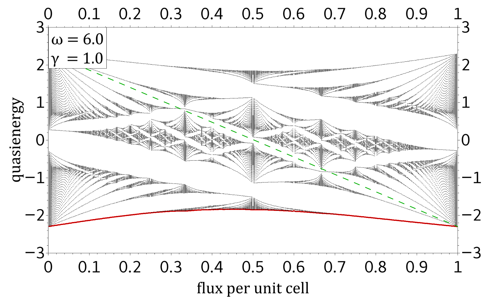
Figure 3: The Hofstadter butterfly gets deformed in presence of circularly polarized light. The frequency $\omega$ of the periodic driving was set to $6.0\,g/\hbar$ and the intensity $\gamma$ to $1.0\,eAa/\hbar$. With the present choice of frequency the different butterflies of the different Floquet modes do not overlap. The red line shows the state with lowest quasienergy of the central Floquet mode.

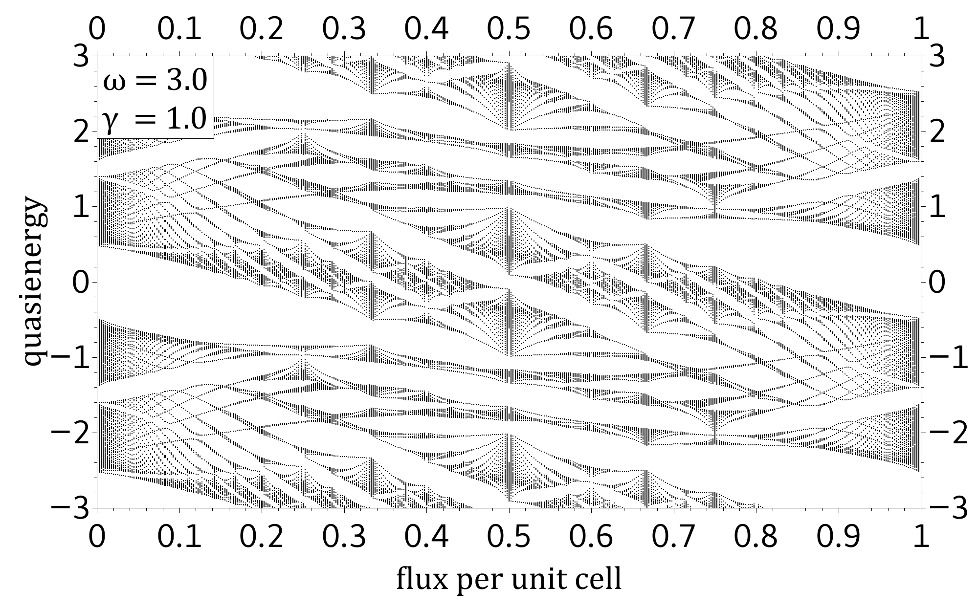
Figure 4: The frequency $\omega$ of the circularly polarized radiation was set to $3.0\,g/\hbar$ and the intensity $\gamma$ to $1.0\,eAa/\hbar$. The spectra of the different Floquet modes overlap.

III.2 Linearly polarized light

We investigate now the case of linear polarization of the light represented by

$$\vec{A}(\vec{r},t)=\begin{pmatrix}A_{x}\cos(\omega t)\qquad\ \ \ \\ A_{y}\cos(\omega t)+Bx\end{pmatrix}\ .$$ (34)

The orientation of the linear polarization can be tuned by varying $A_{x}$ and $A_{y}$. The effective amplitude for the three different hopping paths is then governed by

$$\vec{A}(t)\cdot\vec{a}_{i}=A_{i}\cos(\omega t)\quad\text{with}\quad i=1,2,3\ .$$ (35)

In contrast to the case of circularly polarized light, where the transitions between the different Floquet modes are for all hopping directions equally suppressed, they are for linear polarization not. This can be seen from the fact that the argument of the Bessel function is different for each hopping direction. The equivalent equations to Eqs. (31) and (32) for linearly polarized light read

$$\begin{aligned} &l\hbar\omega\alpha_{n,l}-g\sum_{l^{\prime}}\biggl{[}\Bigl{(}J_{l^{\prime}}(\gamma_{1})\beta_{n,l-l^{\prime}}\\ &+J_{l^{\prime}}(\gamma_{2})e^{i\pi\phi(n-\frac{1}{6})+i\vec{k}\cdot(\vec{b}_{1}-\vec{b}_{2})}\\ &+J_{l^{\prime}}(\gamma_{3})e^{-i\pi\phi(n-\frac{1}{6})-i\vec{k}\cdot\vec{b}_{2}}\Bigr{)}\beta_{n-1,l-l^{\prime}}\biggr{]}=\varepsilon\alpha_{n,l}\;,\end{aligned}$$ (36)

$$\begin{aligned} &l\hbar\omega\beta_{n,l}-g\sum_{l^{\prime}}\biggl{[}\Bigl{(}J_{l^{\prime}}(\gamma_{1})\alpha_{n,l+l^{\prime}}\\ &+J_{l^{\prime}}(\gamma_{2})e^{-i\pi\phi(n+\frac{5}{6})-i\vec{k}\cdot(\vec{b}_{1}-\vec{b}_{2})}\\ &+J_{l^{\prime}}(\gamma_{3})e^{i\pi\phi(n+\frac{5}{6})+i\vec{k}\cdot\vec{b}_{2}}\Bigr{)}\alpha_{n+1,l+l^{\prime}}\biggr{]}=\varepsilon\beta_{n,l}\;.\end{aligned}$$ (37)

Here, we have introduced three different light parameters

$$\gamma_{i}=\frac{eA_{i}a}{\hbar}\ .$$

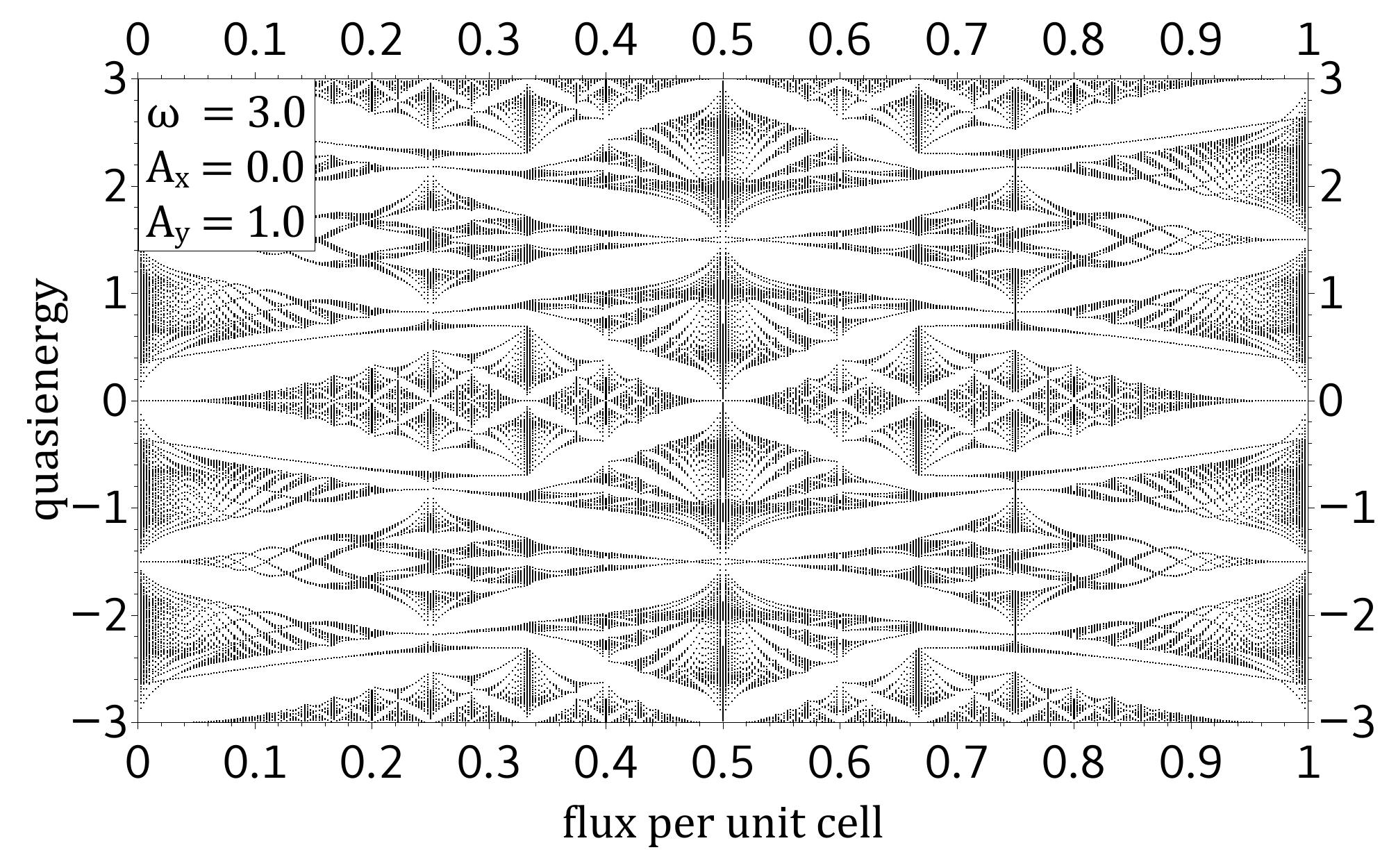
Figure 5: Hofstadter butterfly in presence of linearly polarized light where $A_{x}=0.0\,,\,A_{y}=1.0$ at a frequency $\omega$ of $3.0\,g/\hbar$. The effective amplitude for each hopping direction is governed by Eq. (35).

One should note that particle hole symmetry is conserved for linear light polarization, whereas it is not for circular polarization.

III.3 Gap size

To prepare for the following section, where we analyze the Chern numbers of the static Hofstadter and the Floquet-Hofstadter problem, we investigate the gap size occurring between the different Floquet-Butterfly modes. To do so, we first clarify what is meant by the gap between the different butterflies. We always calculate the gap size numerically between the lowest band of the central Floquet mode, being in the interval $[-\hbar\omega/2,\hbar\omega/2)$, and the highest band of the minus one Floquet mode, lying in $[-3\hbar\omega/2,-\hbar\omega/2)$ . Due to the periodicity of the Floquet-Hofstadter spectrum on the quasienergy axis the gap between neighboring modes is always the same. It is obvious that the quasienergetic gap is not equal for all flux values, e.g., in Fig. 3 the lowest band of the central Floquet mode is not constant as a function of the flux per unit cell.

As already mentioned, we focus on Chern numbers in the following section. A change of the Chern number is always related to a band touching. Hence, we are interested in the minimal gap as a function of flux, denoted as $\Delta\varepsilon$ in Fig. 6, 7, and 8. We refer to a gap between the butterflies if there is no flux value where the lowest band of the central Floquet mode and the highest band of the $n=-1$ mode touch.

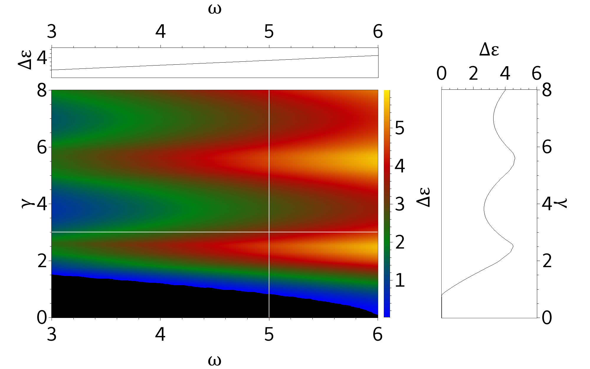
Figure 6: The gap $\Delta\epsilon$ of the Floquet-Hofstadter spectrum as a function of frequency $\omega$ and intensity $\gamma$ for circularly polarized light. In the investigated intensity range two maxima occur rising linearly with the driving frequency.

The right plots of Fig. 6, 7, and 8 show cuts through the contour plot at a frequency of $5.0\,g/\hbar$. The upper plots show cuts at an intensity of $3.0\,eAa/\hbar$. We can see that the gap size rises linearly with the frequency. In anticipation to the following section, we can state that the change of Chern numbers for $\omega=6.0\,g/\hbar$ is for all polarizations only induced by band touchings of butterfly bands lying in the same Floquet zone and not by touching of bands from different Floquet modes.

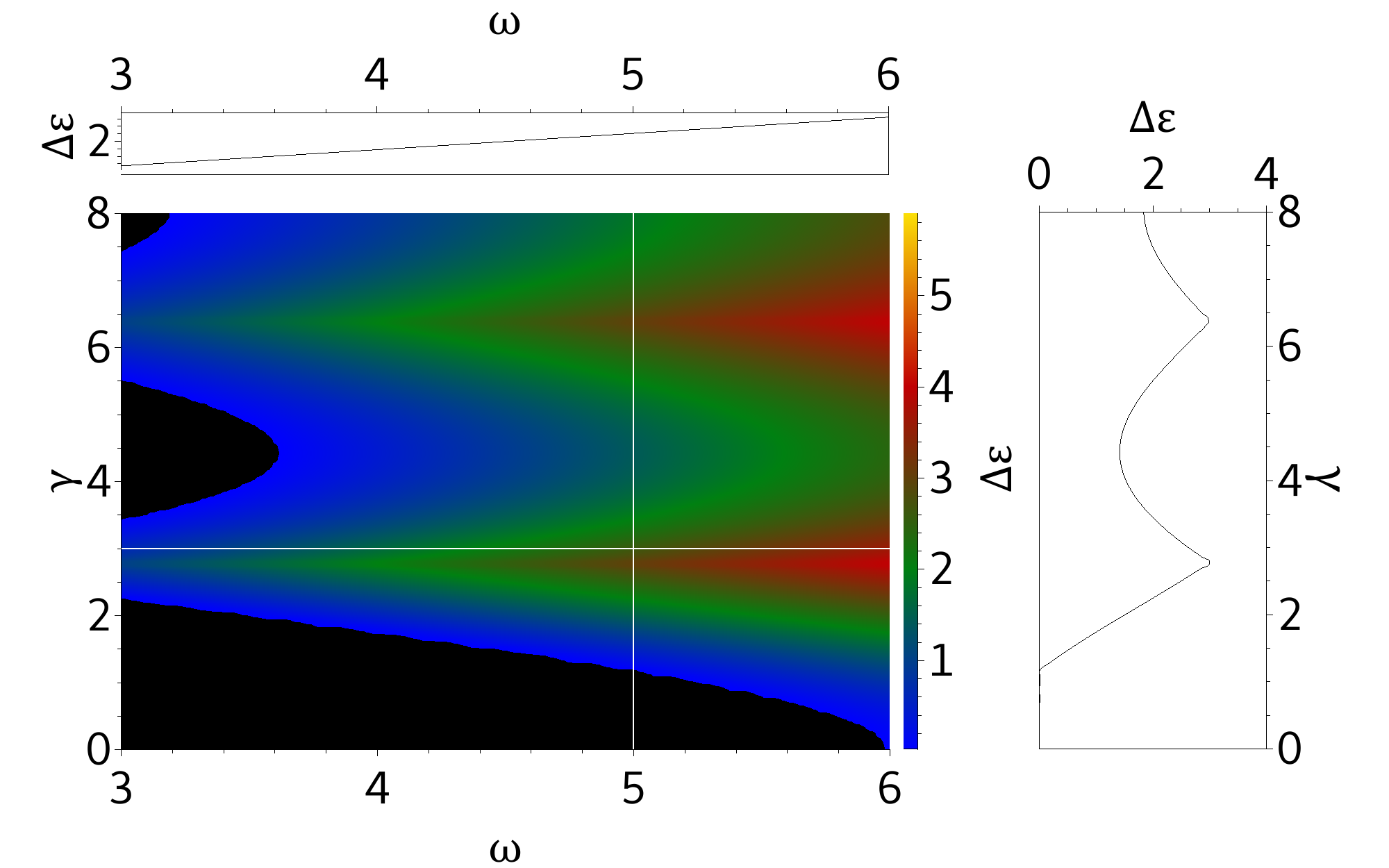
Figure 7: The polarization shows in $y$-direction. The gap shows qualitatively a similar behavior as for circularly polarized light but the gap is overall smaller.

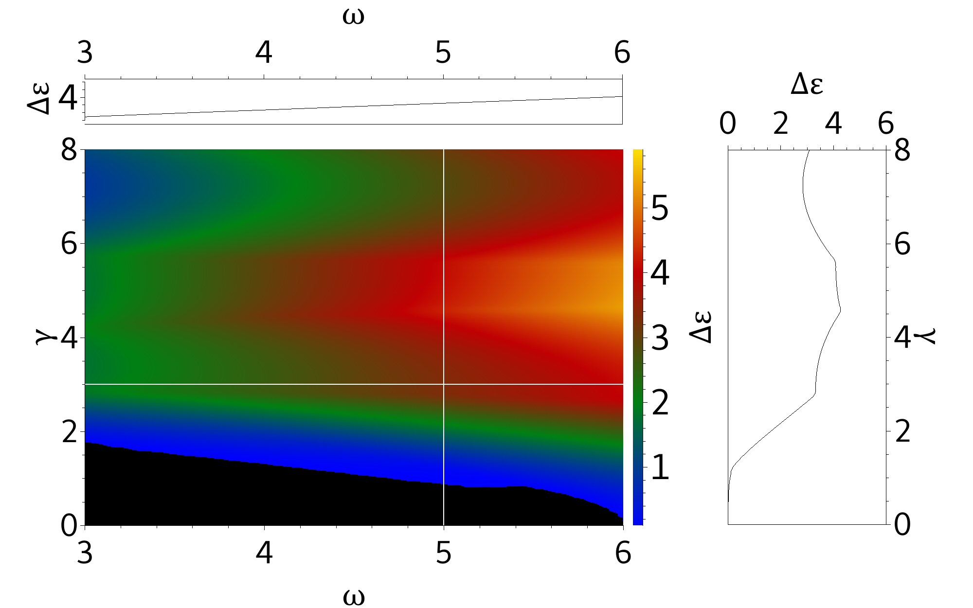
Figure 8: The polarization was set in $x$-direction, parallel to the $\vec{a}_{1}$ bonding. The two gap maxima at $\gamma=2.75\,eAa/\hbar$ and $\gamma=6.4\,eAa/\hbar$ at $\omega=5.0\,g/\hbar$ for $y$-polarization move together when changing the polarization into the $x$-direction.

IV Topological Characterization

IV.1 Chern numbers

Now, we turn to the topological characterization of the Hofstadter bands Thouless et al. (1982); Höckendorf et al. (2018, 2017); Nathan and Rudner (2015); Wang and Li (2016), focusing first on Chern numbers. This topological invariants can be defined for quantum states with two periodic parameters. They are calculated by an integral of the Berry curvature $\vec{F}$ over a two-dimensional compact surface $\mathcal{T}^{2}$, in this case the BZ in the quasienergy space of $H_{F}$: Since the eigenstate $\ket{\alpha,\vec{k},t}$ with $H_{F}\ket{\alpha,\vec{k},t}=\varepsilon_{\alpha}\ket{\alpha,\vec{k},t}$ is periodic in time we can, according to Eq. (29), also formally write

$$\ket{\alpha,\vec{k},t}={} \sum_{n}e^{in\omega t}\ket{u_{\vec{k}\alpha}^{n}}\;,$$ (38)

where $\alpha$ refers to a band index within one Floquet replica $n$. The Chern number associated to a Floquet band $\alpha$ with a Floquet state $\ket{u_{\vec{k}\alpha}^{n}}$ and quasienergy $\varepsilon_{\vec{k}\alpha}$ is given by

$$C_{\alpha}={} \frac{1}{2\pi}\int_{\text{BZ}}\mathrm{d}^{2}k\,\vec{F}_{\alpha}(\vec{k})\cdot{\hat{z}}\;,$$ (39)

with the Berry curvatureThouless et al. (1982); Berry (1984); Simon (1983) given by

$$\vec{F}_{\alpha}(\vec{k})={} \sum_{\beta\neq\alpha}\mathrm{Im}\frac{\braket{u_{\vec{k}\alpha}^{n}}{\vec{\nabla}_{\vec{k}}H_{F}}{u_{\vec{k}\beta}^{n}}\times\braket{u_{\vec{k}\beta}^{n}}{\vec{\nabla}_{\vec{k}}H_{F}}{u_{\vec{k}\alpha}^{n}}}{(\varepsilon_{\vec{k}\alpha}-\varepsilon_{\vec{k}\beta})^{2}}\;.$$ (40)

As long as the Floquet space is not truncated $\vec{F}_{\alpha}(\vec{k})$ does not depend on the Floquet mode $n$. The effect of a truncation of the Floquet space will be discussed in Sec. IV.2.

Following Goldman Goldman (2009), we concentrate on the state of lowest energy in one Floquet mode at given flux per unit cell as indicated in Fig. 2. The Chern number is calculated numerically by the method proposed by Fukui et al., Ref. Fukui et al., 2005. Fig. 9 reproduces the data of Ref. Goldman, 2009 and extends it to a larger number of different flux values $\phi=p/q$.

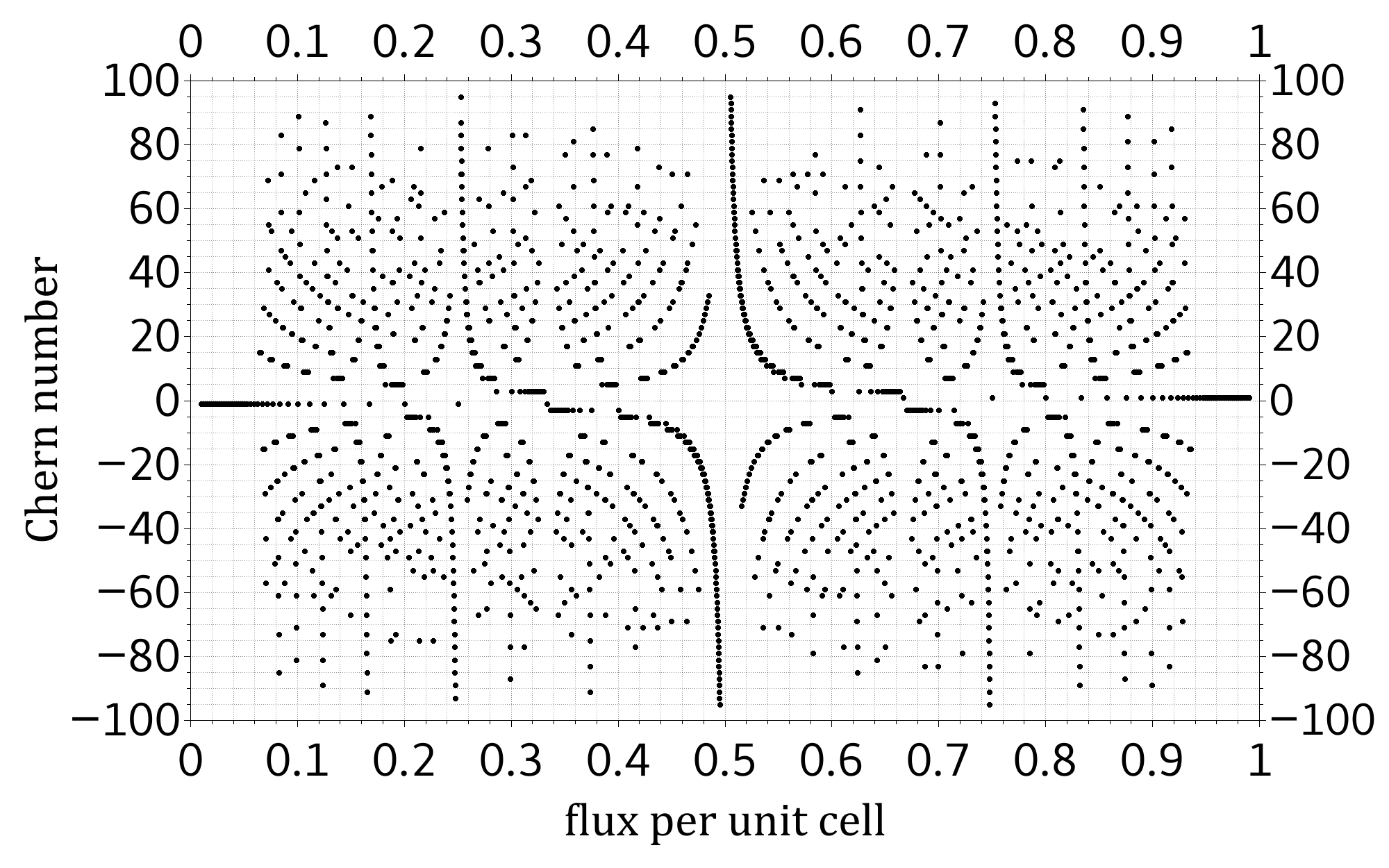
Figure 9: The Chern number of the state of lowest energy of the Hofstadter butterfly in dependence of the magnetic flux per unit cell. The flux values are all $p/q$ with $p$ co-prime to $q<101$.

The computation is effectively limited by the fact that with growing $q$ (being coprime to $p$) energy bands move closer to each other and are increasingly difficult to resolve, an effect which is most pronounced at fluxes near zero and unity. From a numerical perspective the bands are degenerate impeding the use of the computation scheme by Fukui et al. constructed for non-degenerate band structures.

Next, we analyze how polarized light affects the Chern numbers of the Hofstadter butterfly. First, let us consider the case of circularly polarized light. The basis for this analysis are the Eqs. (31) and (32). At high frequencies the Hofstadter butterflies of the different Floquet modes are quasienergetically separated since the distance of the Floquet modes is governed by the photon energy. Hence, the change of Chern numbers is induced by band touchings within the Floquet zone, as can be seen in Fig. 6, 7, and 8. At frequencies large compared to the hopping energy the butterfly spectrum has an overall gap in a broad intensity range. For intensities considered in this section the topological phase transitions are all due to band touchings within the same Floquet mode. Again, we concentrate on the state of lowest quasienergy in the central Floquet mode, see Fig. 3. With the Eqs. (31), (32) we were able to reproduce several results of Mikami et al., Ref. Mikami et al., 2016, in the limit of vanishing magnetic field strength.

As already stressed in several worksMikami et al. (2016); Seetharam et al. (2015); Desbuquois et al. (2017) the distribution function in a driven system is in general not an equilibrium distribution function. Despite that the Chern number maintains its significanceMikami et al. (2016) keeping in mind that one needs another topological invariant to fully characterize a driven system Rudner et al. (2013). We use the term ground state as the state with lowest quasienergy of the central Floquet mode, emphasizing that we do not touch the question of the occupation of the Floquet modes in general. However, we assume that the ground state depends adiabatically on the intensity at least in the high frequency regime. As long as the driving is far from resonances the driving does not significantly change the ground state and with that the distribution function. This also requires that the driving must not induce a heating of the system. Hence, if we only occupy the ground state of the static system we also assume that in the off resonantly driven system only the ground state is occupied.

Our Chern number computations are done in the off-resonant frequency regime. Hence, the ground state of the driven system undergoes the topological phase transitions presented in Fig. 10, 11, and 12. For a vanishing light parameter $\gamma$ and high frequencies, the ground state Chern numbers are the same as in the undriven case, see Fig. 9.

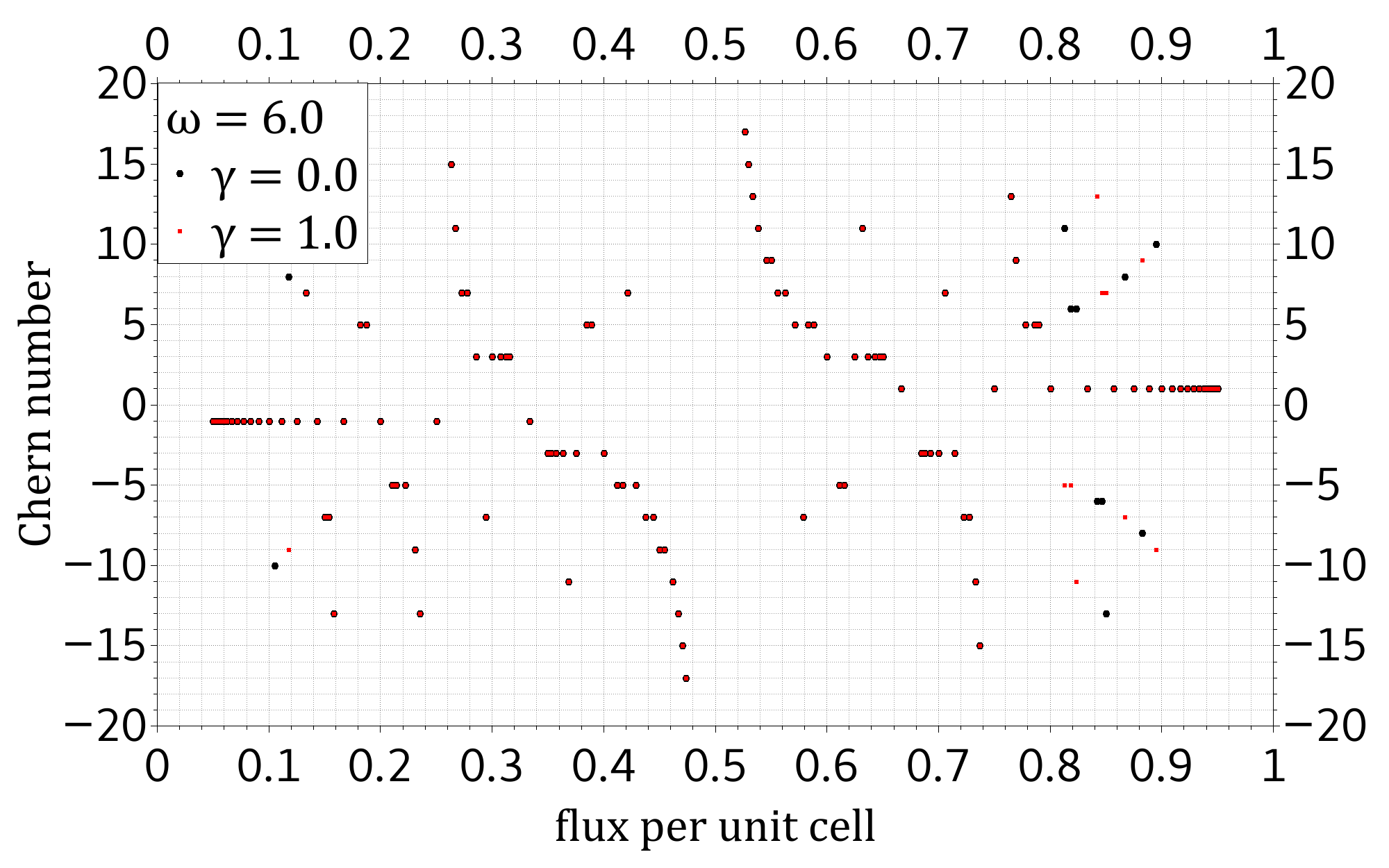
Figure 10: The ground state Chern number of the Floquet-Hofstadter spectrum: The frequency $\omega$ of the circularly polarized light was set to $6.0\,g/\hbar$. The black values show the case of vanishing light intensity $\gamma$ and the red values are calculated for an intensity of $1.0\,eAa/\hbar$.

In Fig. 10 most Chern numbers coincide with the case of a vanishing intensity. When the intensity is further increased the ground state Chern number exhibits a rather different behavior. Even small intensity changes can have a vast influence on the Chern number Mikami et al. (2016), see Fig. 11. Since the Floquet-Hofstadter spectrum gets twisted in presence of circularly polarized light and keeps particle-hole symmetry for linearly polarized light it is obvious that the band structure of graphene is differently affected for the two polarization states. The deformation of the band structure and the associated gap closing and opening is related to the change of Chern numbers. Hence, we investigate as well the influence of linearly polarized light on the distribution of Chern numbers. Similar to the case of circularly polarized light, for rather small intensities only few Chern numbers deviate from the static Chern number distribution. An increase of the intensity leads to a significantly different behavior, as shown in Fig. 12.

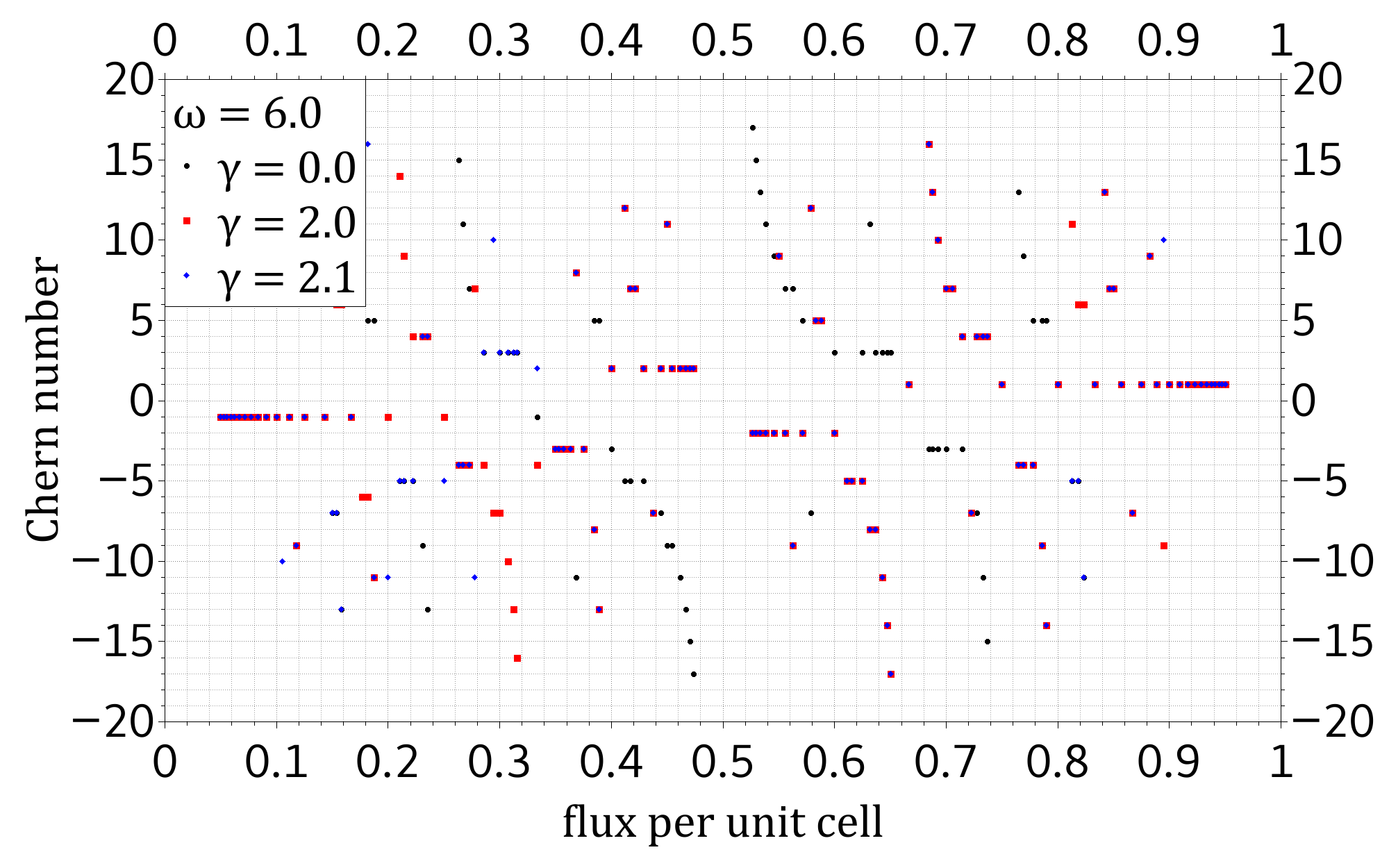
Figure 11: The distribution of the ground state Chern number in presence of circularly polarized light exhibits for intensities $\gamma$ of $2.0\,eAa/\hbar$ and $2.1\,eAa/\hbar$ a rather different behavior as for vanishing intensity. The plot shows flux values for $q<21$.

For circularly polarized light the ground state is uniquely defined. Whereas, for linearly polarized light this is not the case for all flux values. At flux values of, e.g., $6/11$, $6/13$ or $3/17$ a band crossing of the ground state occurs. This effect can be seen at eight different flux values for $q<21$. The occurrence of the band crossing of the ground state seems not to follow a simple rule.

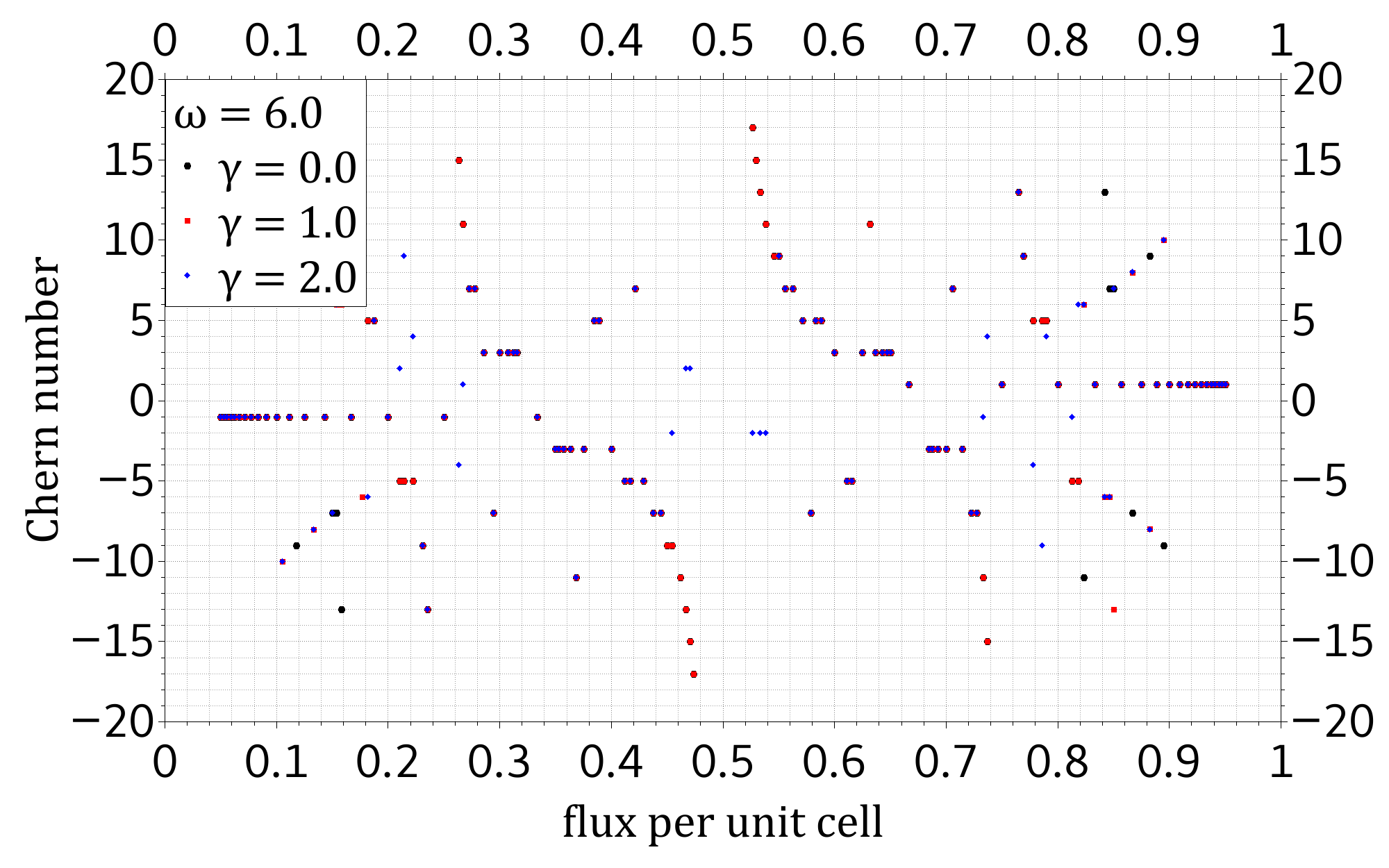
Figure 12: In the case of linear polarization with $A_{x}=0.0,A_{y}=\gamma$ the distribution of the Chern number is for linearly polarized light similar affected as for circularly polarized light. The frequency $\omega$ was again fixed at $6.0\,g/\hbar$ and the intensity is governed by Eq. (35).

IV.2 $W_{3}$-invariants

The topological invariant $\nu_{3}$ associated with the third homotopy group of the periodic unitary maps $\{U_{\vec{k}}(T)\}$ is given in $\mathbb{R}^{3}$ by

$$\nu_{3}[U_{\vec{k}}]={} \frac{1}{24\pi^{2}}\int_{\text{BZ}}\mathrm{d}^{3}k\,\varepsilon_{\alpha\beta\gamma}\,\mathrm{tr}\big{[}(U^{-1}_{\vec{k}}(T)\partial^{\alpha}U_{\vec{k}}(T))$$

$$\cdot(U^{-1}_{\vec{k}}(T)\partial^{\beta}U_{\vec{k}}(T))(U^{-1}_{\vec{k}}(T)\partial^{\gamma}U_{\vec{k}}(T))\big{]}\;.$$ (41)

Rudner et al., Ref. Rudner et al., 2013, have devised an invariant specifically designed for the characterization of periodically driven systems. The idea is to replace in Eq. (41) one $k$-dimension with the time and choose a unitary matrix $\tilde{U}_{\vec{\mu}}$ which is periodic in time and topologically equivalent to a time evolution operator $U_{\vec{\mu}}$,

$$W_{3}[\tilde{U}_{\vec{\mu}}]={} \frac{1}{24\pi^{2}}\int_{[0,1)^{3}}\mathrm{d}^{3}\mu\,\varepsilon_{\alpha\beta\gamma}\,\mathrm{tr}\big{[}(\tilde{U}_{\vec{\mu}}^{-1}\partial^{\alpha}\tilde{U}_{\vec{\mu}})$$

$$\cdot(\tilde{U}_{\vec{\mu}}^{-1}\partial^{\beta}\tilde{U}_{\vec{\mu}})(\tilde{U}_{\vec{\mu}}^{-1}\partial^{\gamma}\tilde{U}_{\vec{\mu}})\big{]}\;,$$ (42)

where the cube $[0,1)^{3}$ is spanned by two normalized in-plane wave vectors and the time $t/T$ with $\vec{\mu}\in[0,1)^{3}$. The indices $\alpha$, $\beta$, $\gamma$ are given modulo 3 and $\partial^{\alpha}\equiv\partial^{\mu_{\alpha}}$. This new invariant is related to the lowest quasienergy gap in the central Floquet mode. The relation between the $W_{3}$ invariants of different gaps $\xi_{n}$ with $\exp(i\xi_{n})\in\mathbb{S}^{1}$ around quasienergies $\varepsilon_{\nu}$ is closely related to Chern numbers $C^{\nu}$ of appropriate bands $\nu$. It is given byHöckendorf et al. (2017)

$$W_{3}[\tilde{U},\xi_{b}]={} W_{3}[\tilde{U},\xi_{a}]-\sum_{\nu=\nu_{1},\ldots,\nu_{k}}C_{\nu}^{(3)}\Big{|}_{\mu_{3}\equiv\frac{t}{T}=1}\;,$$ (43)

where the bands $\nu_{1},\ldots,\nu_{k}$ are the bands one passes through when the value $\xi$ changes from gap at $\xi=\xi_{a}$ to the gap at $\xi=\xi_{b}$. The Chern number is calculated byHöckendorf et al. (2017)

$$C_{\nu}^{(\alpha)}={} \frac{1}{2\pi i}\int_{0}^{1}\int_{0}^{1}\mathrm{d}\mu_{\alpha-1}\mathrm{d}\mu_{\alpha+1}\,[\epsilon_{\alpha\beta\gamma}(\partial^{\beta}(S^{\dagger}\partial^{\gamma}S))]_{\nu\nu}\;,$$ (44)

where $C_{\nu}^{(3)}|_{\mu_{3}=1}$ is equivalent to Eq. (39). The columns of the matrix $S$ contain the eigenvectors of $U_{\vec{\mu}}$. Clearly, the full computation of the invariant constructed in Ref. Rudner et al., 2013 is more complicated Höckendorf et al. (2017) than for Chern numbers Fukui et al. (2005).

The calculation scheme suggested by Rudner et al., Ref. Rudner et al., 2013, in frequency space is described in the following. In order to calculate the generalized topological invariant for driven systems one first computes the Chern number of all bands below the investigated gap of a truncated Floquet matrix. The generalized invariant is then given by the sum off all Chern numbers below this gap. In Fig. 5 in Ref. Rudner et al., 2013 the lowest band of the truncated Floquet matrix has a Chern number $C_{0}$ different from $C_{F}$. The reason why that Chern number is not $C_{F}$ is due to the truncation. As already shown by ShirleyShirley (1963, 1965), from the Fourier expansion in Eq. (38) it follows that the corresponding eigenvector to a quasienergy $\varepsilon_{\lambda}$ differs from the eigenvector of the quasienergy $\varepsilon_{\lambda}+\hbar\omega$ only by an index shift of the entries and a phase $\phi$ which one is free to chooseShirley (1963)

$$\varepsilon_{\lambda}\leftrightarrow\begin{pmatrix}\vdots\\ u_{\lambda}^{-2}\\ u_{\lambda}^{-1}\\ u_{\lambda}^{0}\\ u_{\lambda}^{1}\\ u_{\lambda}^{2}\\ \vdots\end{pmatrix}\Longleftrightarrow\varepsilon_{\lambda}+\hbar\omega\leftrightarrow e^{i\phi}\begin{pmatrix}\vdots\\ u_{\lambda}^{-3}\\ u_{\lambda}^{-2}\\ u_{\lambda}^{-1}\\ u_{\lambda}^{0}\\ u_{\lambda}^{1}\\ \vdots\end{pmatrix}\;,$$ (45)

where $\lambda$ labels a discrete set of quantum numbers, e.g., spin or sublattice degrees. This holds equivalently for arbitrary shifts $n\hbar\omega$, with $n\in\mathbb{Z}$, of the quasienergy. It shows that the Chern number $C_{\varepsilon_{\lambda}}$ of a band described by $\varepsilon_{\lambda}$ has to be equal to the Chern number of the shifted band

$$C_{\varepsilon_{\lambda}}=C_{\varepsilon_{\lambda}+n\hbar\omega}\,.$$ (46)

This means for the numerics that if we assume that only a finite number of eigenvector entries are different from zero we have to choose the truncation of the Floquet modes large enough in order to achieve convergence of these. Let us assume that we have to limit the number of Floquet modes to $m$ in order to achieve convergence of the central quasienergy $\varepsilon_{\lambda}$ up to a needed precision. If the eigenvector corresponding to $\varepsilon_{\lambda}\pm m\hbar\omega$ is computed this eigenvalues and eigenvectors are in general not converged leading to different results in the quasienergy spectrum as well as Chern numbers. To sum up, these non converged Chern numbers might lead to an incorrect topological characterization. Indeed, Höckendorf et al. give a counterexample in Ref. Höckendorf et al., 2017 where the summation over Chern numbers suggested by Rudner et al. Rudner et al. (2013) fails to give the correct $W_{3}$-invariant. The authors consider a spin-$1/2$ rotation described by the Hamiltonian

$$H_{w}=2\pi w\,\vec{f}(\mu_{1},\mu_{2})\cdot\vec{\sigma}$$ (47)

together with the corresponding time evolution operator

$$U(\vec{\mu})=e^{-iH\mu_{3}}\;,$$ (48)

where the $\mu_{i}$ are chosen as in Eq. (42), $w\in\mathbb{Z}$ and the function $\vec{f}$ is a map from the square to the unit sphere $\vec{f}:[0,1]^{2}\rightarrow\mathbb{S}^{2}$. For further details we refer to Ref. Höckendorf et al., 2017. The corresponding two bands have Chern number $\pm 1$, whereas $W_{3}=2w$. Despite the fact that the Hamiltonian $H$ is time-independent, the system exhibits a nontrivial topology when investigating its time evolution. We are now in the position to clarify why the summation over Chern numbers proposed by Rudner et al. fails for this example. If we apply Floquet theory to the Hamiltonian (47) with vanishing driving amplitude and frequency $\omega=2\pi/T$, we create Floquet copies identical to the undriven system. This implies that the Chern numbers of the two bands in each Floquet zone are equal to the Chern numbers of the undriven system, i.e., they are $\pm 1$. Therefore, summing over all Floquet copies yields a topological invariant of zero in contrast to the correct $W_{3}$-invariant of $2w$. The above mapping $\vec{f}(\mu_{1},\mu_{2})$ can be easily constructed by concatenating three different mappings. The first one is shifting and stretching the square

$$\vec{s}(\vec{\mu}) :[0,1]^{2}\to[-1,1]^{2}$$ (49)

$$\vec{s}(\vec{\mu}) :\begin{pmatrix}\mu_{1}\\ \mu_{2}\end{pmatrix}\mapsto\begin{pmatrix}2\mu_{1}-1\\ 2\mu_{2}-1\end{pmatrix}\ .$$ (50)

The second one is a map from a square to a circle

$$\vec{c}(\vec{\mu}) :[-1,1]^{2}\to\{|\vec{\mu}|\leq 1:\vec{\mu}\in\mathbb{R}^{2}\}$$ (51)

$$\vec{c}(\vec{\mu}) :\begin{pmatrix}\mu_{1}\\ \mu_{2}\end{pmatrix}\mapsto\begin{pmatrix}\mu_{1}\sqrt{1-\tfrac{\mu_{2}^{2}}{2}}\\ \mu_{2}\sqrt{1-\tfrac{\mu_{1}^{2}}{2}}\\ \end{pmatrix}$$ (52)

and the third one maps a circle to a sphere

$$\vec{b}(\vec{\mu}) :\{|\vec{\mu}|\leq 1:\vec{\mu}\in\mathbb{R}^{2}\}\to\{|\vec{\mu}|=1:\vec{\mu}\in\mathbb{R}^{3}\}$$ (53)

$$\vec{b}(\vec{\mu}) :\begin{pmatrix}\mu_{1}\\ \mu_{2}\end{pmatrix}\mapsto\begin{pmatrix}\frac{\mu_{1}}{n}\sin(\pi n)\\ \frac{\mu_{2}}{n}\sin(\pi n)\\ \cos(\pi n)\end{pmatrix}$$ (54)

with $n=\sqrt{\mu_{1}^{2}+\mu_{2}^{2}}$. This finally yields the sought mapping $f$,

$$\vec{f}(\mu_{1},\mu_{2})=\vec{b}\big{(}\vec{c}\big{(}\vec{s}(\vec{\mu})\big{)}\big{)}\ .$$ (55)

Let us now consider the case $w=1$. The operator in Eq. (48) can be interpreted as a time evolution operator of a time-independent Hamiltonian

$$H_{w=1}=\frac{2\pi}{T}\vec{f}(\mu_{1},\mu_{2})\cdot\vec{\sigma}\;,$$ (56)

which has however a trivial but periodic time evolution with a period $T=1$. Note that the eigenvector matrix $\Lambda$ of $H_{w=1}$ allows for the transformation

$$\Lambda\vec{f}(\mu_{1},\mu_{2})\cdot\vec{\sigma}\Lambda^{\dagger}=\sigma^{z}\;.$$ (57)

Rudner et al., Appendix C in Ref. Rudner et al., 2013, made the attempt to map all time-independent flat band Hamiltonians onto

$$H_{P}(\vec{\mu})=\frac{2\pi}{T}P(\vec{\mu})\;,$$ (58)

with $P(\vec{\mu})$ being a projection operator. The authors were able to show that for these class of Hamiltonians the $W_{3}$-invariant $W_{3}[U]$ is equal to the Chern number of the bands with quasienergy $\varepsilon=-2\pi/T$. One should stress that the quasienergies of a Hamiltonian of the form (58) are degenerate everywhere whereas the Chern numbers are still defined. But there is a class of flat band Hamiltonians which cannot be mapped onto $H_{P}$. One example is $H_{w=1}$ since the spectra differ. Here, the mentioned relation between the $W_{3}$-invariant and the Chern number fails. Furthermore, very much as in Appendix C, one can show that the quasienergies of the Floquet Hamiltonian corresponding to Eq. (56) are both zero and thus degenerate everywhere. Nevertheless, the Chern numbers are $\pm 1$ and summation over these will never lead to the same number of edge modes as predicted by $W_{3}=2$. This shows that the summation over Chern numbers of the truncated Floquet Hamiltonian is not justified for every system. Another example is discussed in Appendix C. Despite this counterexamples, the summation over Chern numbers over the truncated Floquet matrix and the calculation of the $W_{3}$-invariant for graphene without magnetic field show a striking accordance, see Appendix B.

In order to assure the correctness of the topological invariant we applied the algorithm proposed by Höckendorf et al., Ref. Höckendorf et al., 2017, to compute numerically the $W_{3}$-invariant for the Floquet-Hofstadter spectrum at $p/q=1/3$. The result is plotted in Fig. 15.

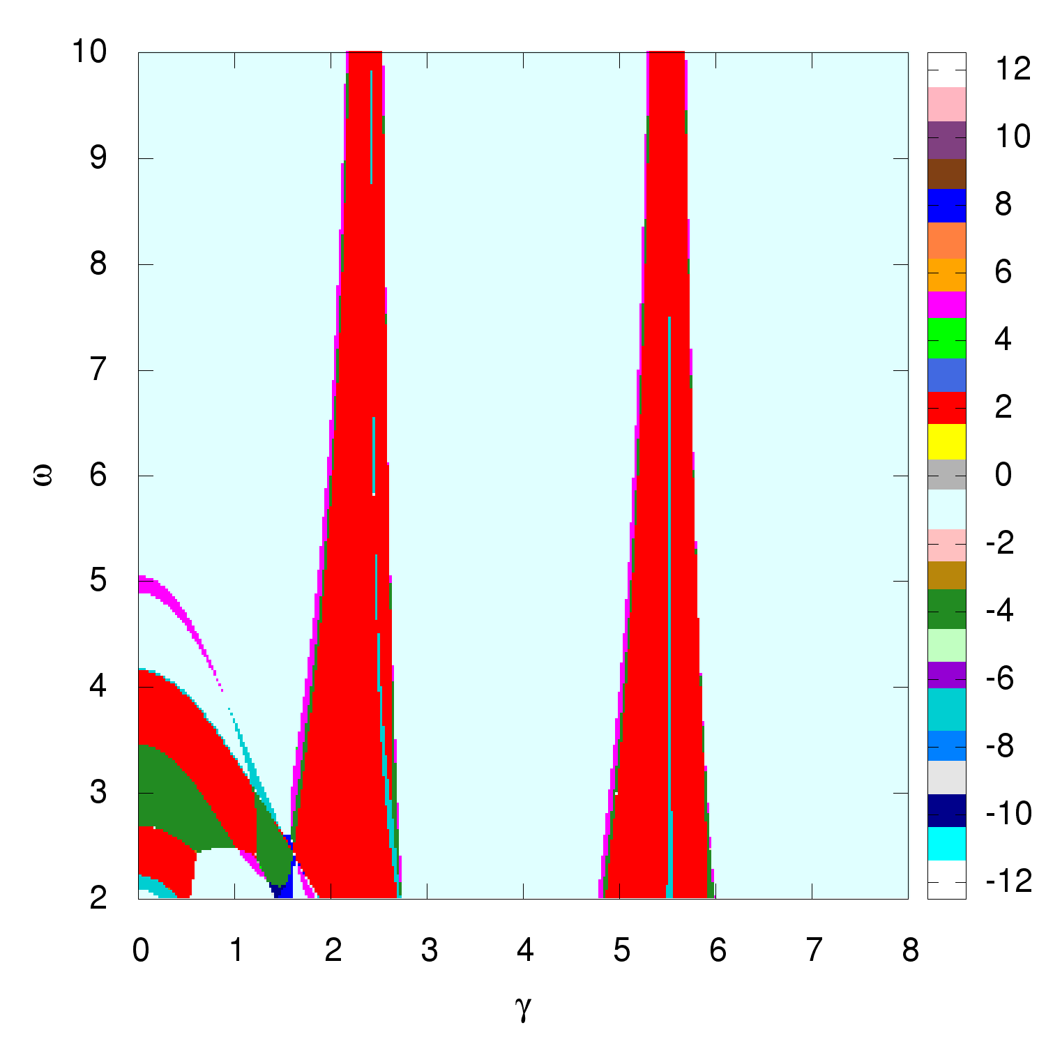
Figure 13: The Chern number of the state with lowest energy of the central Floquet zone for a flux per unit cell of $p/q=1/3$ and circularly polarized driving.

To have a comparison to the static topological invariants, we first compute the Chern number of the state with lowest energy of the central Floquet zone for a flux per unit cell of $p/q=1/3$ and circularly polarized driving. The three dimensional momentum-time BZ is discretized by 200$\times$200$\times$200 points together with 30 Floquet replicas. The resulting Chern numbers are plotted in Fig. 13 for different amplitudes $\gamma$ and frequencies $\omega$ of the driving field. In the left lower region of Fig. 13, inside the arc from $(\gamma,\omega)=(0.0\,eAa/\hbar,5.1\,g/\hbar)$ to $(\gamma,\omega)=(1.9\,eAa/\hbar,2.0\,g/\hbar)$, we can not trust the numerical values. The reason can be understood by investigating the band structure. In the parameter space where $\hbar\omega<6.0\,g$ the bands of the Floquet-Hofstadter spectrum overlap and the Chern numbers are not well defined. With rising intensity the degeneracies are lifted and anticrossings occur. Moreover, there are $(\gamma,\omega)$ regions where no gap between the lowest and the second lowest exists but the bands are nowhere degenerate, see Appendix A.

In the last step we apply the $W_{3}$ calculation scheme following Ref. Rudner et al., 2013 as mentioned before. The same flux and polarization is used as for Fig. 13. The result is plotted in Fig. 14. In the following, we compare the results of both $W_{3}$ calculations and contrast them against the corresponding Chern numbers.

The difference between both results for the $W_{3}$-invariant is depicted in Fig. 16. The comparison shows that apart from zones close to topological phase transitions the results coincide.

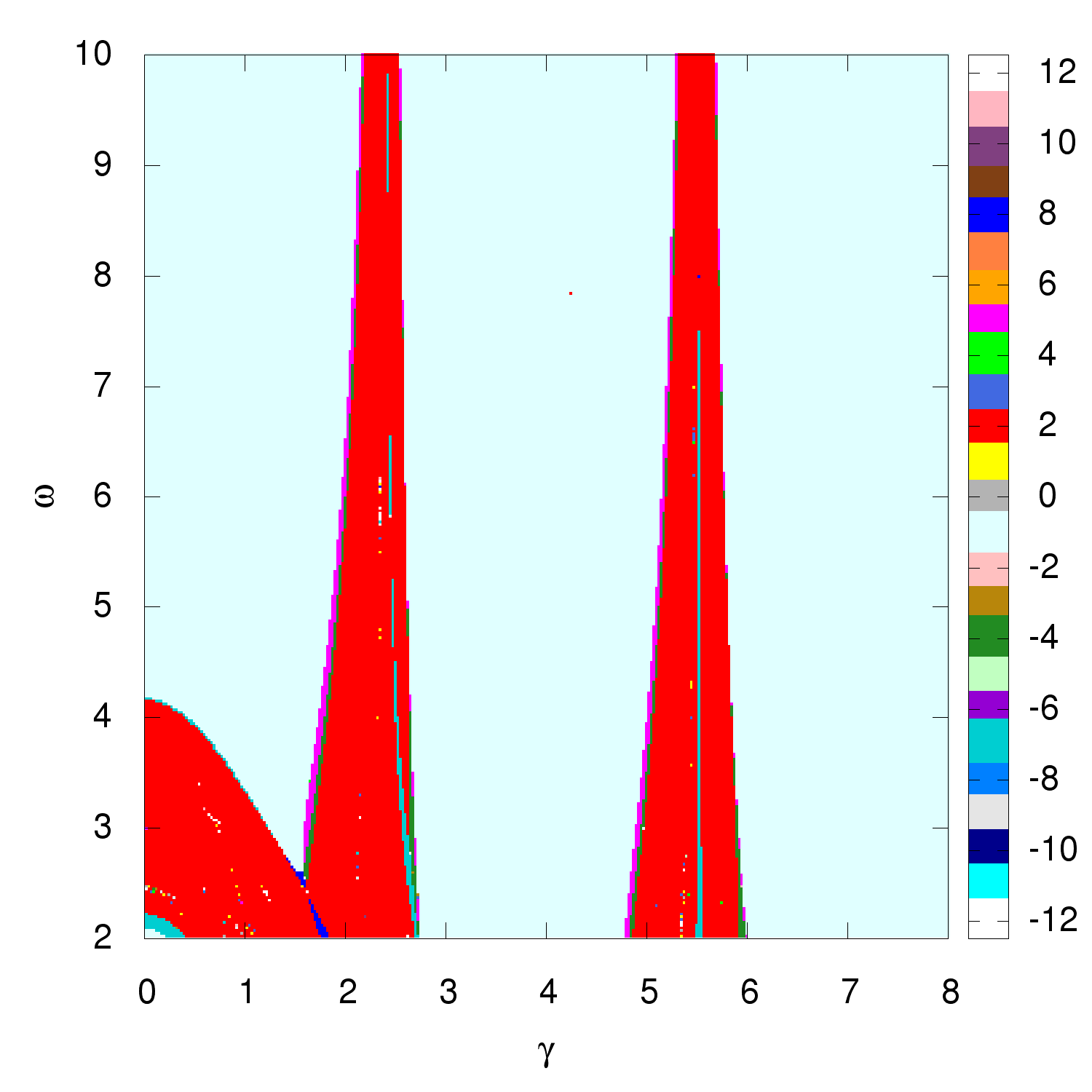
Figure 14: The sum over all Chern numbers below $\varepsilon=0$ computed from the truncated Floquet Hamiltonian with the same flux and polarization as in Fig. 13 and Fig. 15.

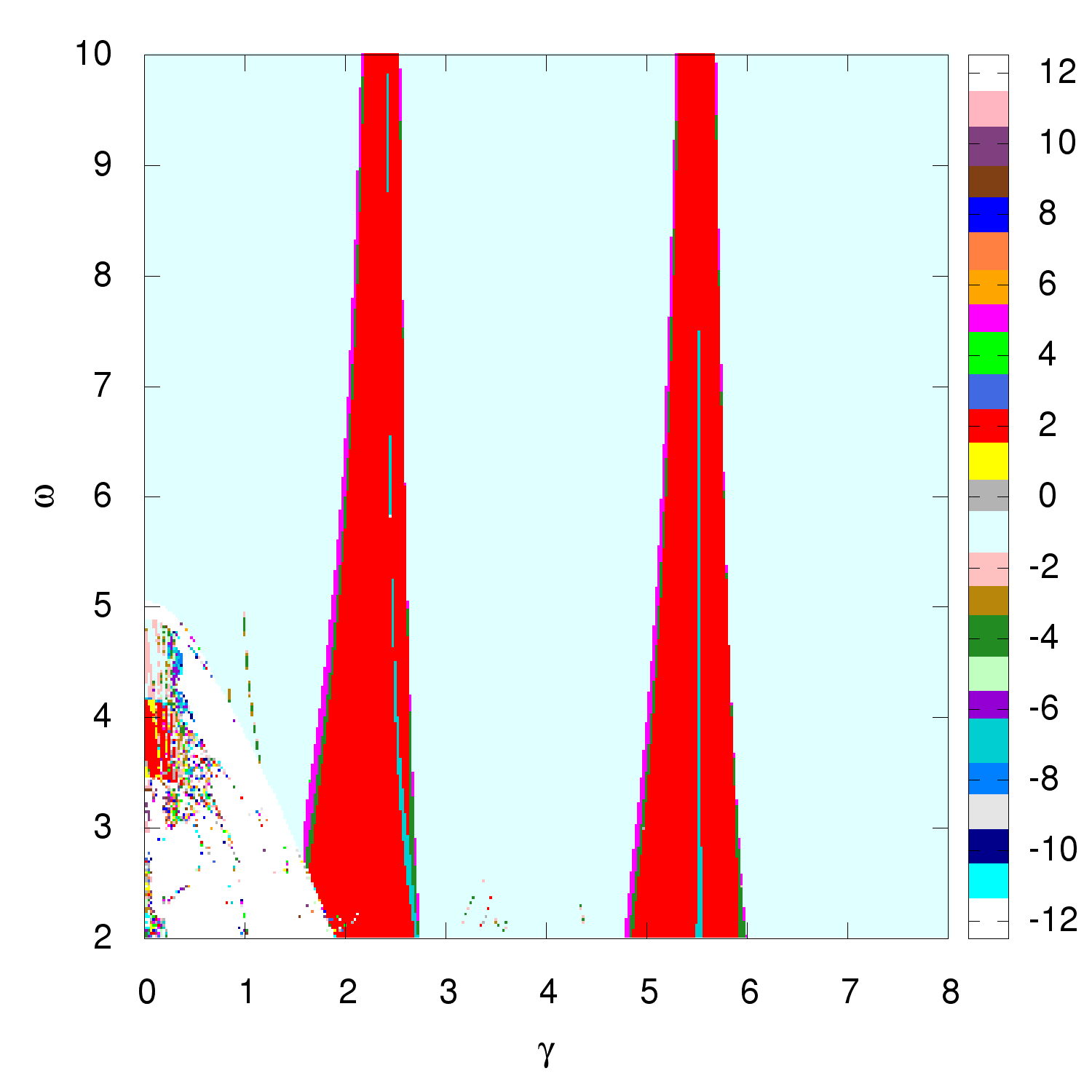
Figure 15: The $W_{3}$-invariant computed with the algorithm by Höckendorf et al.Höckendorf et al. (2017) for the Floquet-Hofstadter spectrum at $p/q=1/3$. The driving was circularly polarized.

Interestingly, the Chern number itself show as well a great agreement with both the sum over the Chern numbers and $W_{3}$. This justifies once more the topological characterization presented in Sec. IV.1. Using the connection between edge modes and the $W_{3}$-invariant which has been proven in Ref. Rudner et al., 2013, this result allows for the prediction of the number of edge modes in this driven system.

Furthermore, we would like to stress that although the here presented topological characterization is different from the one presented in Ref. Kooi et al., 2018 by Kooi et al. the Chern numbers for a flux per unit cell of $p/q=1/3$ agree with our results up to the sign of the $W_{3}$-invariants due to a different sign choice of the driving frequency.

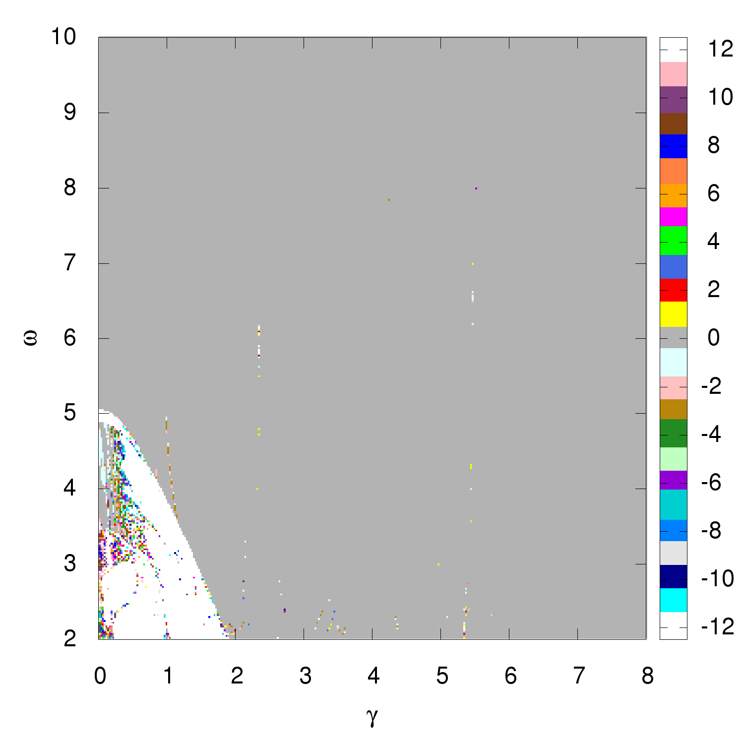
Figure 16: The difference between the sum over Chern numbers and the $W_{3}$-invariant. Grey regions show parameter configurations $(\gamma,\omega)$ where the Chern number sum and the $W_{3}$-invariant coincide.

V Summary

In this paper we presented an explicit and rigorous treatment of the Hofstadter problem on the hexagonal lattice. One important result is the explicit proof of the periodicity of the Hofstadter butterfly: Depending on whether the numerator of the flux per unit cell is even or odd the periodicity of the fractal spectrum is different. To understand how illumination of graphene with both circularly and linearly polarized light in presence of a magnetic field will effect the fractal spectrum we unified the Hofstadter butterfly with the Floquet theory. These two polarization modes lead to clearly different scenarios. Circularly polarized light in combination with a magnetic field is able to lift the symmetry of the quasienergy spectrum around zero energy, whereas linearly polarized light is not, as shown by representative data. Furthermore, we investigated the gap size between different Floquet modes of the Floquet-Hofstadter spectrum.

To investigate the topological properties of this dynamical system, we studied the Chern number of the state with lowest quasienergy in the central Floquet mode for different flux values. Limiting the computations to the high frequency regime we were able to identify that the topological phase transitions induced by the external radiation field are only caused by gap closings and openings of butterfly bands and not by touching of different Floquet modes. For vanishing intensity the computed Chern numbers coincide with the ones of the undriven system. Furthermore, we found that the system undergoes several topological phase transitions when tuning the flux per unit cell or the intensity. Thereby the distribution of the Chern numbers changes in presence of an oscillating electric field for both linearly and circularly polarized light similarly. For moderate intensities only few Chern numbers are different from the Chern numbers of the static case whereas for higher intensities the distribution is substantially altered.

Yet, the appropriate invariant to look at in case of a periodically driven system is the $W_{3}$-invariant. We computed this topological indicator for the Floquet-Hofstadter spectrum to give a comparison with the results on Chern numbers. In the high frequency limit both the Chern number and the $W_{3}$-invariant coincide, yielding the correct number of edge modes appearing in a system of finite size. The latter allows for an experimental access. Finally, we were able to show agreement with other topology studies on the Floquet-Hofstadter spectrum in the off resonant regime. Whereas, our topology analysis of the system is valid in all driving regimes, resonant and off resonant.

Appendix A Gapless non-degenerate states

There is a global gap between two bands if the minimum of the upper band is always greater than the maximum of the lower band. Consider the case of two bands without a global energy gap. It does not imply that there is a degeneracy of the two bands. This scenario occurs for specific $(\gamma,\omega)$ configurations of the Floquet Hofstadter spectrum between the lowest and second lowest band marked as black stripes in Fig. 18. An exemplary quasienergy band structure is shown in Fig. 17. There is no gap between the lowest two non degenerate bands.

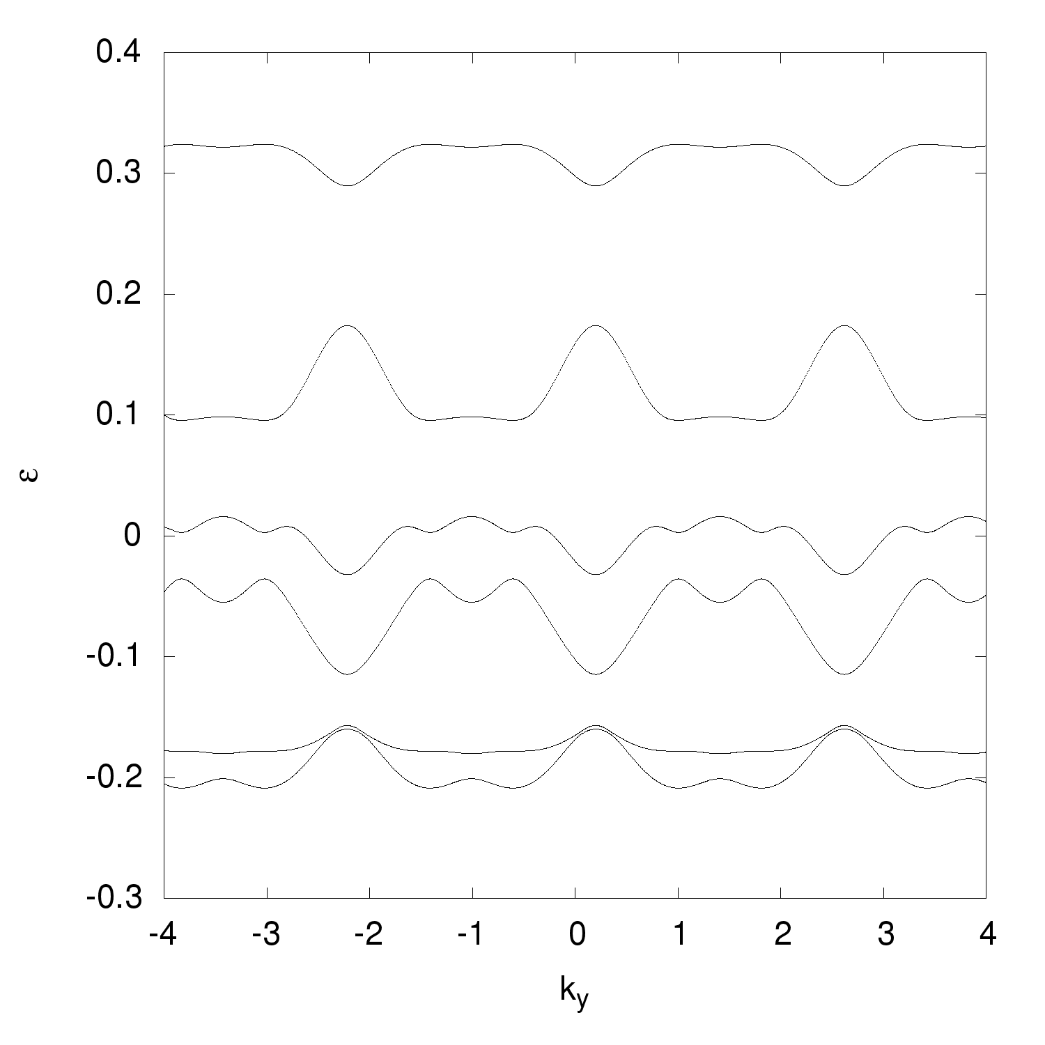
Figure 17: The quasienergy band structure for $p/q=1/3$, $(\gamma,\omega)=(2.65\,eAa/\hbar,3.0\,g/\hbar)$ and $k_{x}=0$. The lowest two bands are not degenerate but they do not have a gap in the sense that the minimum of the second lowest band is always greater than the maximum of the lowest band.

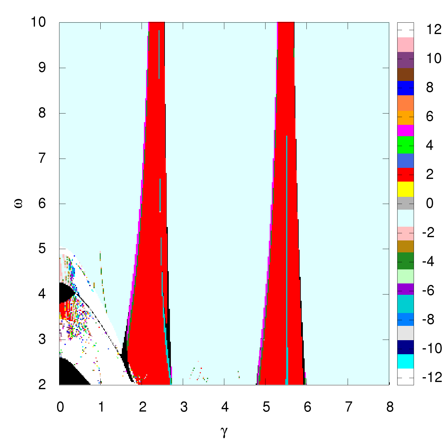
Figure 18: The $W_{3}$-invariant computed with the algorithm of Höckendorf et al.Höckendorf et al. (2017) for the Floquet-Hofstadter spectrum at $p/q=1/3$. The driving was circularly polarized. Parameter spaces $(\gamma,\omega)$ without a gap are marked black.

Appendix B $W_{3}$-invariant for graphene without magnetic field

Although there are examples where the summation over the Chern numbers of the truncated Floquet Hamiltonian fails to give the correct topological invariant, as shown, e.g, by two examples in Ref. Höckendorf et al., 2017, the procedure gives the correct results for several models including circularly polarized driven graphene. In the seminal work by Mikami et al. on Floquet topological insulatorsMikami et al. (2016) the authors were able to relate topological phase transitions to effective hopping amplitudes. Moreover, the topological phase diagram of graphene with circularly polarized driving has been investigated.

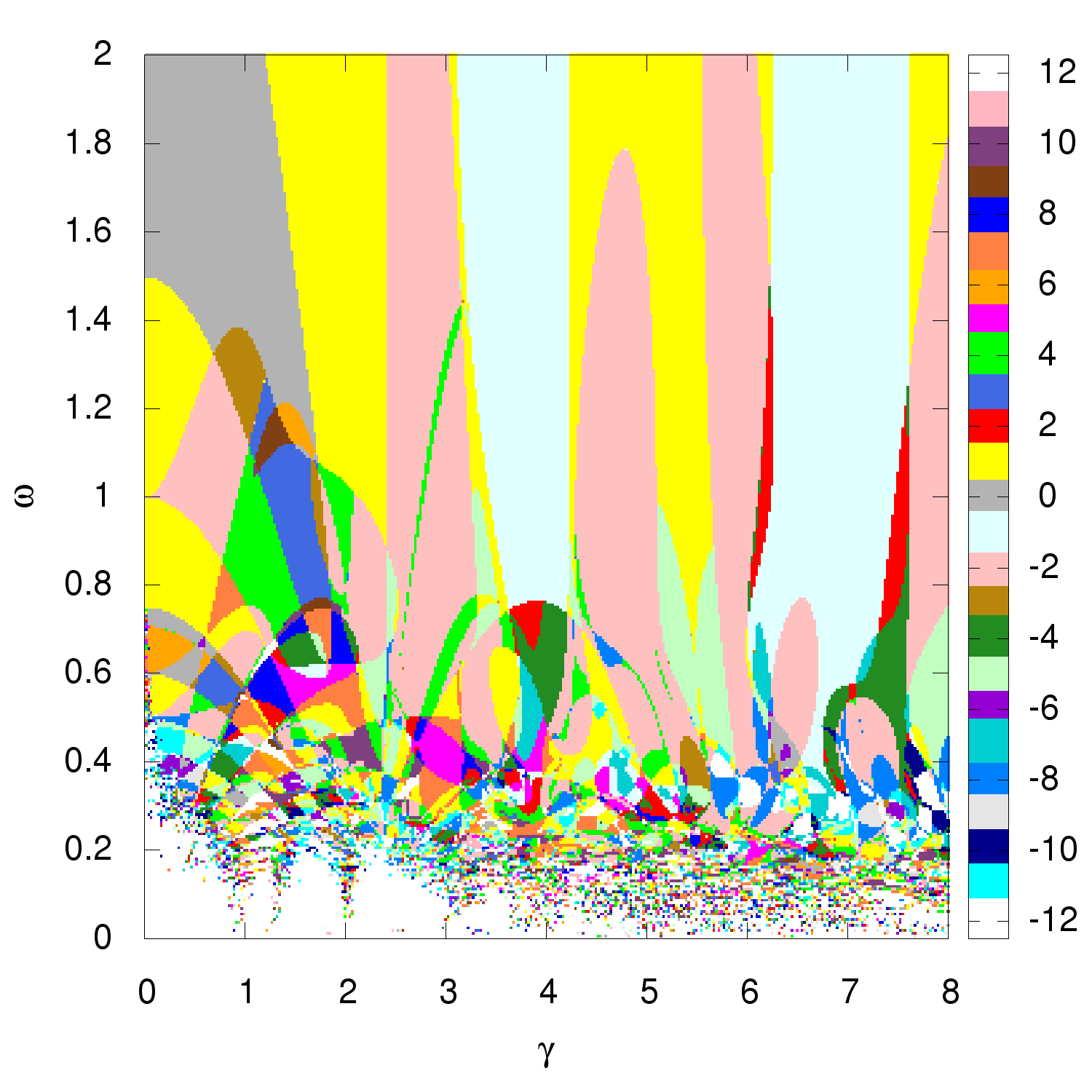
Figure 19: The sum over all Chern numbers of the truncated Floquet Hamiltonian below $\varepsilon=0$ for graphene with circularly polarized driving and without magnetic field. Our data almost perfectly reproduce the results from Ref. Mikami et al., 2016.

In order to make direct contact to the work by MikamiMikami et al. (2016) we have set the discretization of the time-momentum BZ to $200\times 200\times 200$ and the number of Floquet replicas to 50.

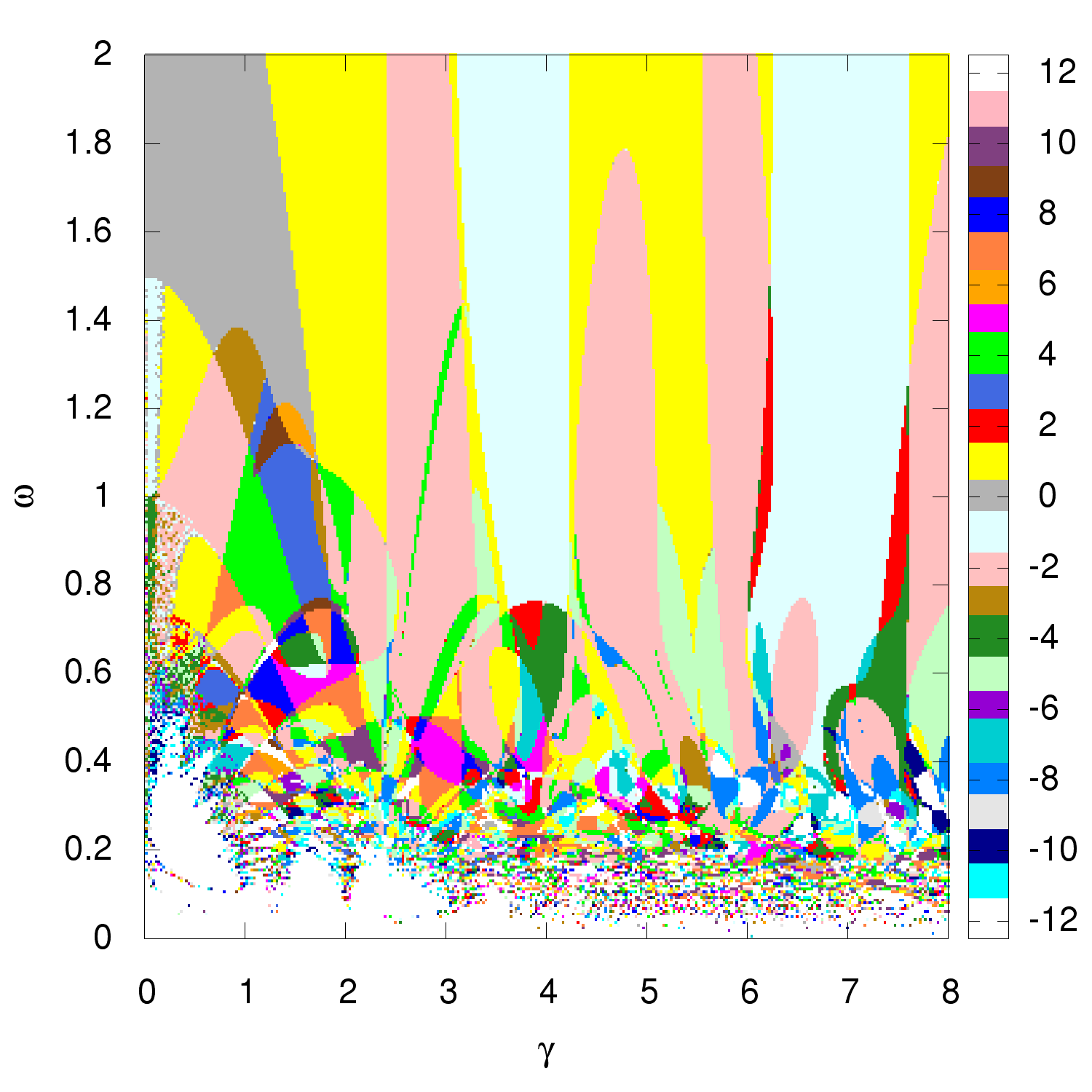
Figure 20: The $W_{3}$-invariant coincides in reliable regions with the sum over Chern numbers. Except for numerical unstable regions the Chern number sum and the $W_{3}$-invariant show a striking agreement.

Although the lowest and topmost eigenvalues and eigenvectors of the truncated Floquet Hamiltonian are not converged, i.e., they are different from the index shifted eigenvectors with eigenvectors taken from the central Floquet zone (compare Eq. (45)) they remain relevant for the topological classification of driven graphene. In the converged Floquet zones the sum over all bands has to be zero inside one specific Floquet zoneHöckendorf et al. (2017). For the lowest and highest Floquet zones this is not necessarily the case. The deviation from the converged Chern numbers contains the information about the difference of Chern numbers and the $W_{3}$-invariants such that the summation gives indeed the correct topological invariant. This can be seen when comparing the sum over all Chern numbers of the truncated Floquet Hamiltonian Fig. 19 with the $W_{3}$-invariant Fig. 20. The difference between the two values is plotted in Fig. 25. In the region of small intensities $\gamma$ and $\hbar\omega<1.5g$ they do not agree. However, this is due to numerical instabilities of the algorithm for the $W_{3}$-invariant. In order to show that there is indeed no difference between the sum over Chern numbers and $W_{3}$ we analyzed the sizes of the gaps at zero quasienergy and $-\omega/2$.

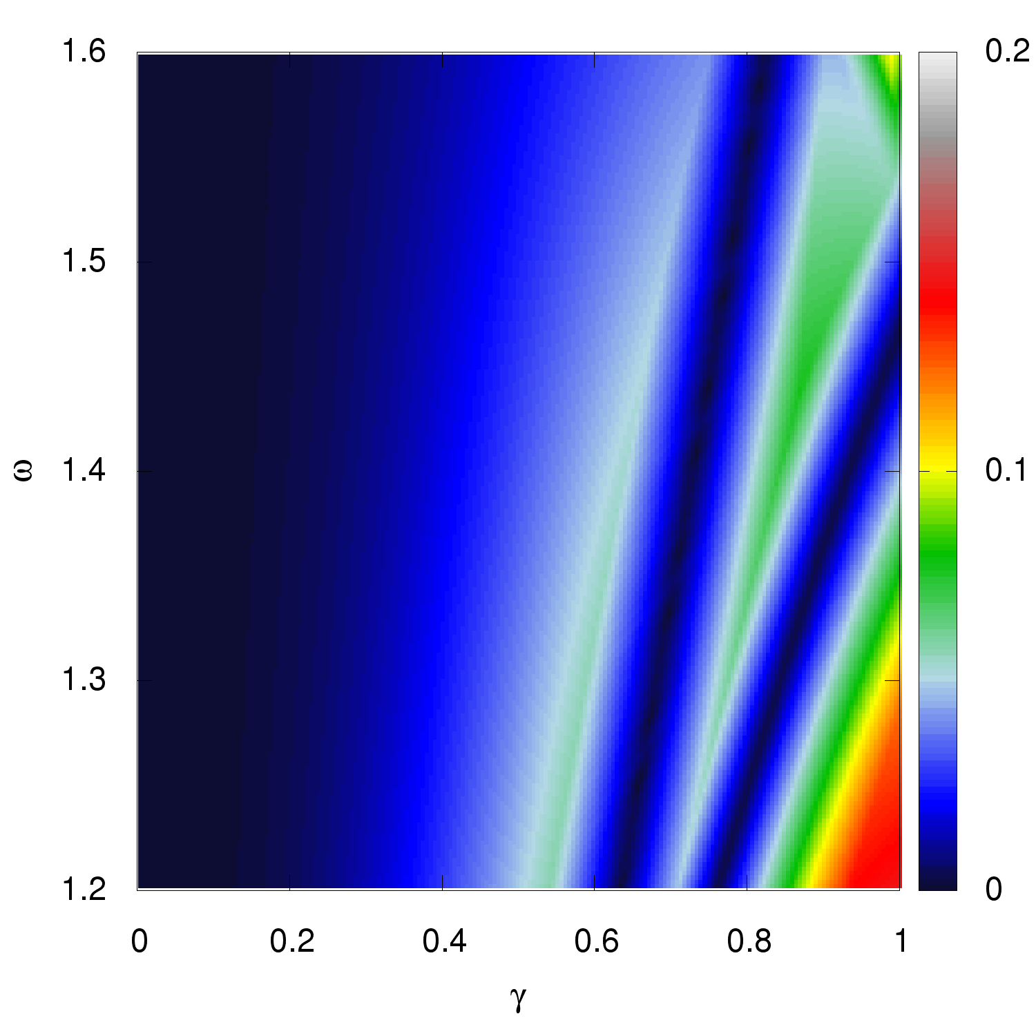
Figure 21: The size of the zone edge gap in dependence of intensity $\gamma$ and driving frequency $\omega$. The data were calculated as distance between the minimum of the lower band of the central Floquet zone and $-\omega/2$. The zero lines at the right half of the plot are also visible as topological phase transition int Fig. 26.

Fig. 21 shows the difference between $-\omega/2$ and the minimum of the lower band of the central Floquet zone. Comparing the regions where the $-\omega/2$-gap is closed with the corresponding regions where the Chern number changes, Fig. 26, one can see that the zeros of the $-\omega/2$-gap are responsible for a change of Chern numbers.

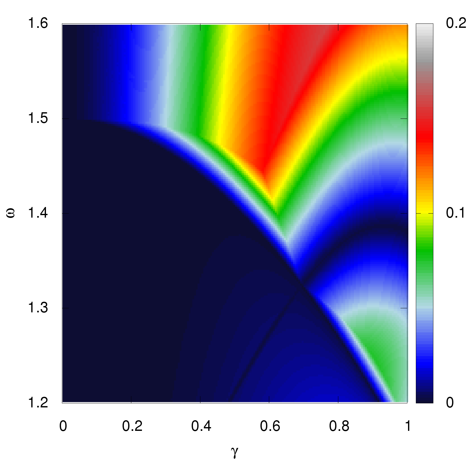
Figure 22: The minimum of the upper band of the central Floquet zone in dependence of intensity $\gamma$ and driving frequency $\omega$ is plotted. The zeros, and with that the band touchings, can be directly mapped to a change of the sum over Chern numbers, compare Fig. 19.

Whereas, the arc in Fig. 22 starting from $(\gamma,\omega)=(0.5\,eAa/\hbar,1.2\,g/\hbar)$ to $(\gamma,\omega)=(1.0\,eAa/\hbar,1.36\,g/\hbar)$, where the zero gap is closed, can be seen in Fig. 20 as well as in Fig. 26.

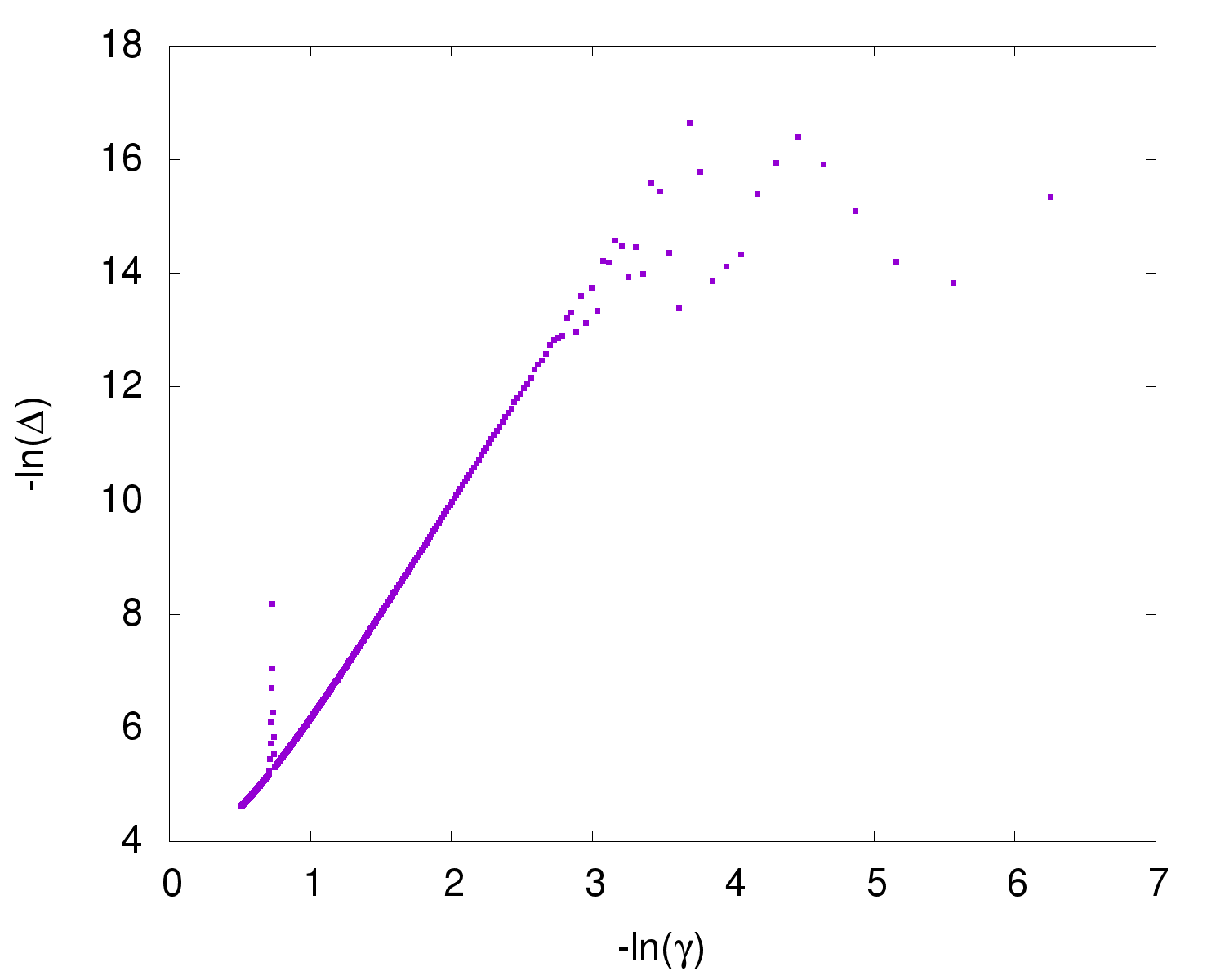
Figure 23: $\Delta$ is the minimum of the upper band of the central Floquet zone and $\gamma$ is here understood as dimensionless intensity $\gamma\to\gamma\,\hbar/eAa$. The plot shows the gap size, i.e., the difference between the minimum of the upper band and zero, for $\gamma=1/520$ to $\gamma=3/5$ at fixed $\omega=1.2\,g/\hbar$. The peak at $-\ln(\gamma)\approx 0.7$ is an evidence for a gap closing at $\gamma=0.5$. Whereas for $-\ln(0.2)\approx 1.6$ no peak is visible, giving a hint that there is no topological phase transition at $\gamma=0.2$.

In the following we clarify if there is a difference between the sum over Chern number of the truncated Floquet Hamiltonian and the $W_{3}$-invariant. We calculated the gap sizes in the interval $\gamma\in[0.0,0.6]\,eAa/\hbar$ for $\omega=1.2\,g/\hbar$. The BZ is discretized by using 3500$\times$3500 points. If there would be a gap closing, e.g, at $(\gamma,\omega)=(0.2\,eAa/\hbar,1.2\,g/\hbar)$ in Fig. 20 we should see a signature of a gap closing either in Fig. 23 or in Fig. 24. The latter show the gap sizes in a double logarithmically plot for the zero and the $-\omega/2$ gap. If there would be a gap closing there should be a signature at $-\ln(\gamma)\approx 1.6$ which is not the case. This shows that the deviations between Chern number summation and $W_{3}$ can be traced back to numerical instabilities. Indeed, we were able to achieve agreement between the results of the summation over Chern numbers and the $W_{3}$-invariant when increasing the discretization of the time-momentum BZ for some representative points. As an example we investigated $(\gamma,\omega)=(0.1\,eAa/\hbar,1.4\,g/\hbar)$: An increase of the number of discretization points to $800\times 800\times 800$ is necessary in order to achieve convergence of the $W_{3}$-algorithm and with that agreement with the summation over Chern numbers.

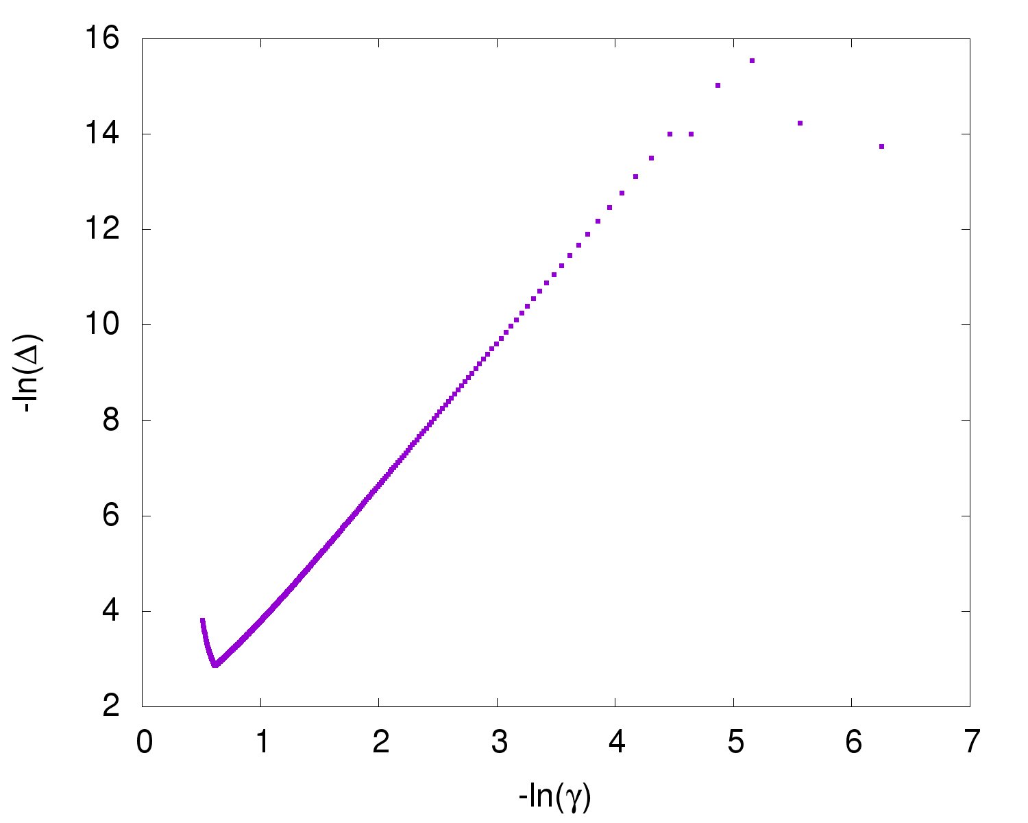
Figure 24: $\Delta$ is the distance between the minimum of the lower band of the central Floquet zone and $-\omega/2$ and, as in Fig. 23, $\gamma$ is again dimensionless. No peak is visible in this plot, where $\gamma$ and $\omega$ are in the same parameter range as in Fig. 23.

Besides from numerical demanding regions, both topological characterizations show a striking agreement, colored with gray in Fig. 25. To our knowledge, apart from the observation that the sum over the Chern numbers of the truncated Floquet Hamiltonian and the $W_{3}$-invariant seem to coincide for circularly driven graphene, a proof, so far, is missing.

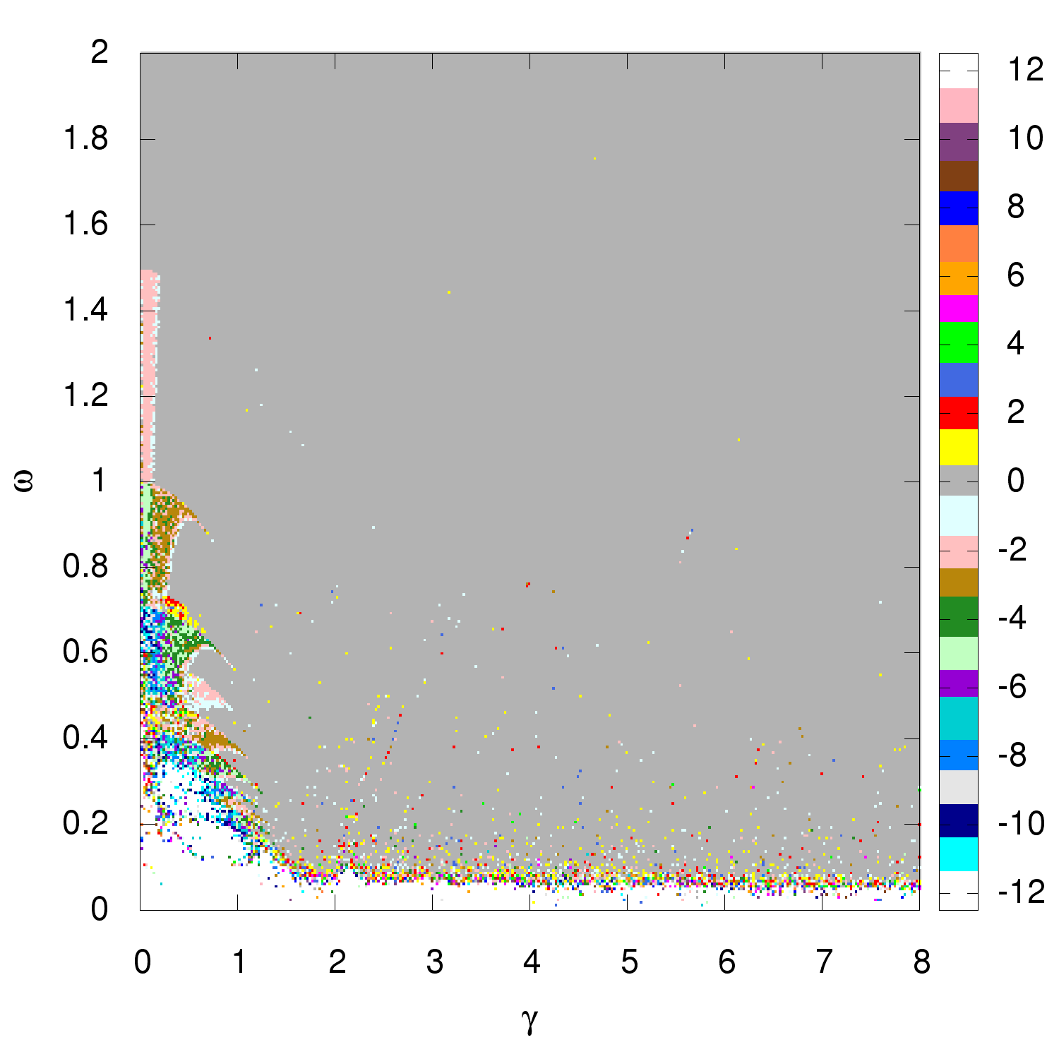
Figure 25: The Difference between the $W_{3}$-invariant and the sum over Chern numbers.

Remarkably, even in the cases where both the Chern number and the $W_{3}$-invariant coincide (e.g., compare $(\gamma,\omega)=(4.0\,eAa/\hbar,2.0\,g/\hbar)$ Fig. 26 and Fig. 20) not all Floquet zones of the truncated Floquet Hamiltonian have the same Chern numbers as the central Floquet zone, as depicted in Fig. 27.

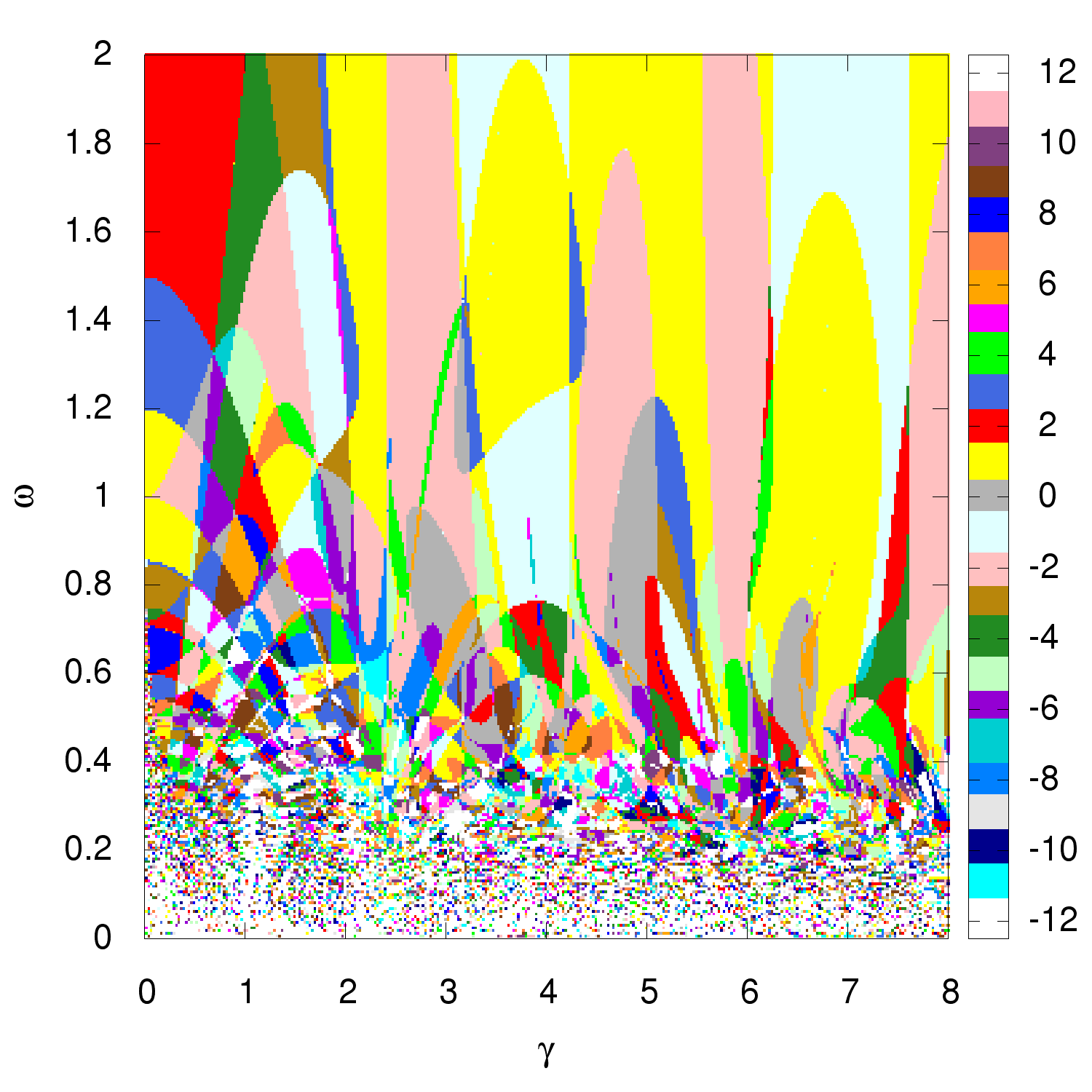
Figure 26: The Chern number of the lower band of graphene of the central Floquet zone. The driving is again circularly polarized. One can see the difference to the $W_{3}$-invariant in Fig. 20.

This holds even for the off resonant regime. Fig. 28 extends Fig. 27 to higher driving frequencies. However, this feature survives for even higher driving frequencies $\omega\propto 10^{6}\,g/\hbar$. Again, this can be understood when having a closer look at the quasienergy band structure. In the far off resonant regime the gap between the two bands of graphene is very small. Hence, even when the Floquet zones are far away from each other a small coupling is enough to close and reopen the small gap of some Floquet zones.

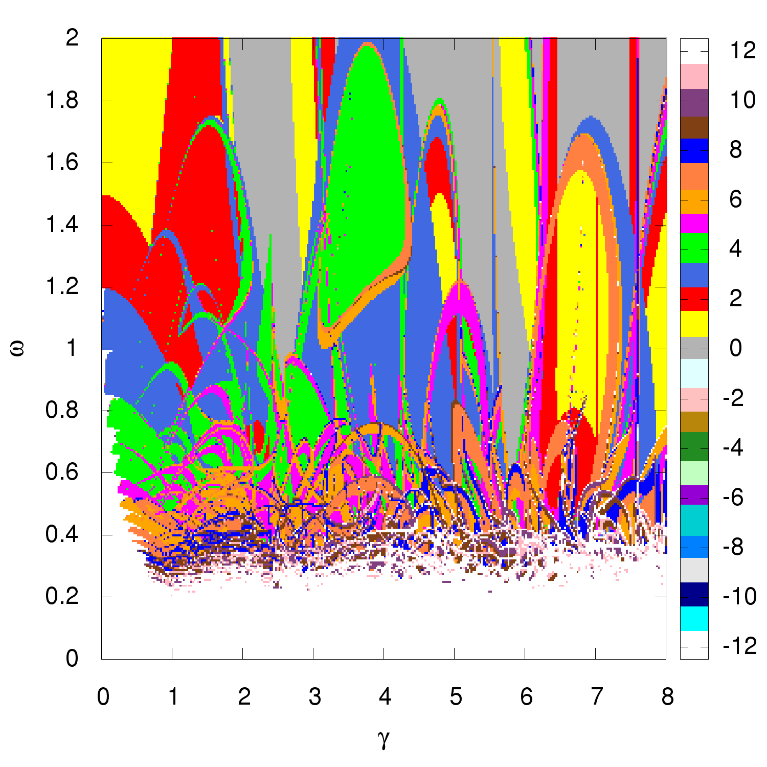
Figure 27: The innermost Floquet zone having different Chern numbers from that of the central Floquet zone. The counting of the Floquet zones starts here with the lowest mode, e.g. for $(\gamma,\omega)=(4.0\,eAa/\hbar,1.6\,g/\hbar)$ the (-50+4)’th Floquet zone has different Chern numbers from the Chern numbers of the central Floquet zone.

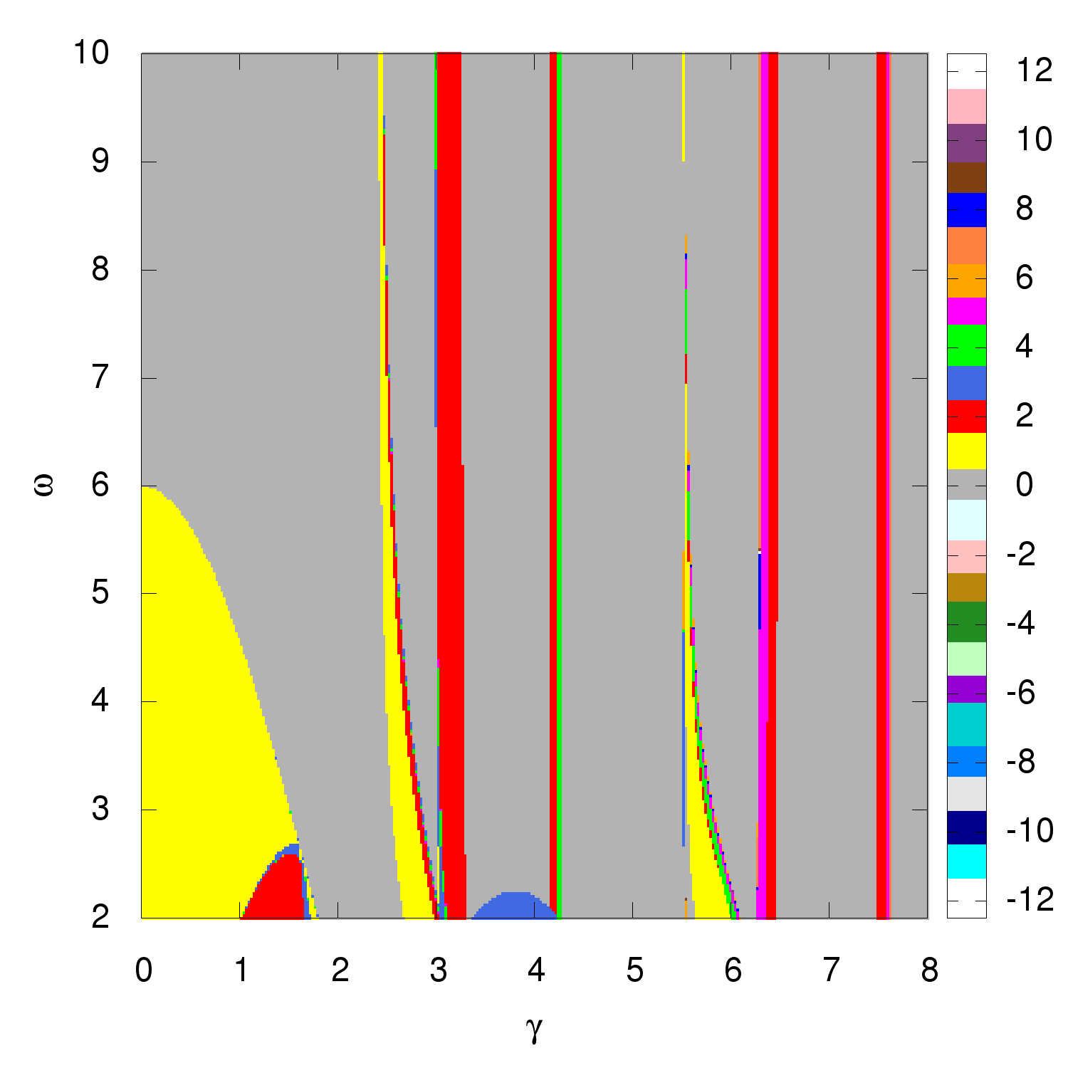
Figure 28: Even in the far off resonant regime not all Chern numbers of the Floquet zones of the truncated Floquet Hamiltonian agree with the Chern numbers of the central Floquet zone.

Appendix C $W_{3}$-invariant for spin-1/2 rotations

Besides the example given in the main text, there is a second case given in Ref. Höckendorf et al., 2017 where the summation over the truncated Floquet Hamiltonian does not give the correct topological invariant in the driven case. In this case the time evolution operator reads

$$U(\vec{\mu})=e^{-i2\pi w\vec{g}(\vec{\mu})\cdot\vec{\sigma}}\;,$$ (59)

where $\vec{g}(\vec{\mu})$ is a bijective map from the cube $[0,1]^{3}$ to the unit ball $|\vec{\mu}|\leq 1$ that maps the surface (center) of the cube to the surface (center) of the unit ballHöckendorf et al. (2017). Let us set $w=1$ in order calculate the $W_{3}$-invariant for one period. The mapping $\vec{g}(\vec{\mu})$ can be constructed by applying two mappings. The first one is shifting the unit cube and stretching it

$$\vec{s}(\vec{\mu}) :[0,1]^{3}\to[-1,1]^{3}$$ (60)

$$\vec{s}(\vec{\mu}) :\begin{pmatrix}x\\ y\\ z\end{pmatrix}\mapsto\begin{pmatrix}2x-1\\ 2y-1\\ 2z-1\end{pmatrix}\;,$$ (61)

and the second one is the mapping to the unit ball

$$\vec{c}(\vec{\mu}) :[-1,1]^{3}\to\{|\vec{\mu}|\leq 1:\vec{\mu}\in\mathbb{R}^{3}\}$$ (62)

$$\vec{c}(\vec{\mu}) :\begin{pmatrix}x\\ y\\ z\end{pmatrix}\mapsto\begin{pmatrix}x\sqrt{1-\tfrac{y^{2}}{2}-z^{2}\big{(}\tfrac{1}{2}-\tfrac{y^{2}}{3}\big{)}}\\ y\sqrt{1-\tfrac{z^{2}}{2}-x^{2}\big{(}\tfrac{1}{2}-\tfrac{z^{2}}{3}\big{)}}\\ z\sqrt{1-\tfrac{x^{2}}{2}-y^{2}\big{(}\tfrac{1}{2}-\tfrac{x^{2}}{3}\big{)}}\end{pmatrix}\ .$$ (63)

By concatenation we yield

$$\vec{g}(\vec{\mu})=\vec{c}\big{(}\vec{s}(\vec{\mu})\big{)}\;.$$ (64)

With the explicit form given for the mapping from the cube to the ball we can calculate the eigenvalues of the operator $\vec{g}(\vec{\mu})\cdot\vec{\sigma}$ which are

$$\lambda_{\pm}=\pm\sqrt{1+64xyz(x-1)(y-1)(z-1)}\ .$$ (65)

By identifying $x\equiv k_{x}$, $y\equiv k_{y}$ and $z\equiv t/T$, the time-dependent Hamiltonian can be reconstructed with

$$H(t)=i\hbar\big{(}\partial_{t}U(t)\big{)}U^{\dagger}(t)\;.$$ (66)

Having $H(t)$ we can calculate the corresponding Floquet-Hamiltonian which has a driving period of $\omega=2\pi$ since we have chosen $w=1$. But we know that the quasienergies $\varepsilon_{\pm}$ of the Floquet Hamiltonian are equal to the eigenvalues of $U(\vec{\mu})$ evaluated after one period, i.e.,

$$\varepsilon_{\pm} =i\ln e^{\pm i2\pi\lambda_{\pm}}\Big{|}_{t/T=1}$$ (67)

$$=\pm 2\pi\;,$$ (68)

and by shifting the quasienergies into the central Floquet zone we get two degenerate bands with zero quasienergy

$$\varepsilon_{\pm}={} 0\;.$$ (69)

The Floquet spectrum is everywhere degenerate but the Chern numbers are well defined. However, the summation over Chern numbers of the truncated Floquet Hamiltonian gives not the correct topological invariant which is in this case $W_{3}=2$.

References

- Klitzing et al. (1980) K. v. Klitzing, G. Dorda, and M. Pepper, Phys. Rev. Lett. 45, 494 (1980).
- von Klitzing (1986) K. von Klitzing, Rev. Mod. Phys. 58, 519 (1986).
- Hasan and Kane (2010) M. Z. Hasan and C. L. Kane, Rev. Mod. Phys. 82, 3045 (2010).
- Qi and Zhang (2011) X.-L. Qi and S.-C. Zhang, Rev. Mod. Phys. 83, 1057 (2011).
- Hofstadter (1976) D. R. Hofstadter, Phys. Rev. B 14, 2239 (1976).
- Thouless et al. (1982) D. J. Thouless, M. Kohmoto, M. P. Nightingale, and M. den Nijs, Phys. Rev. Lett. 49, 405 (1982).
- Fukui et al. (2005) T. Fukui, Y. Hatsugai, and H. Suzuki, J. Phys. Soc. Jpn. 74, 1674 (2005).
- Oka and Aoki (2009) T. Oka and H. Aoki, Phys. Rev. B 79, 081406 (2009).
- Kitagawa et al. (2010) T. Kitagawa, E. Berg, M. Rudner, and E. Demler, Phys. Rev. B 82, 235114 (2010).
- Lindner et al. (2011) N. H. Lindner, G. Refael, and V. Galitski, Nature Physics 7, 490 (2011).
- Gu et al. (2011) Z. Gu, H. A. Fertig, D. P. Arovas, and A. Auerbach, Phys. Rev. Lett. 107, 216601 (2011).
- Cayssol et al. (2013) J. Cayssol, B. Dóra, F. Simon, and R. Moessner, phys. stat. sol. (RRL) 7, 101 (2013).
- Rudner et al. (2013) M. S. Rudner, N. H. Lindner, E. Berg, and M. Levin, Phys. Rev. X 3, 031005 (2013).
- Mikami et al. (2016) T. Mikami, S. Kitamura, K. Yasuda, N. Tsuji, T. Oka, and H. Aoki, Phys. Rev. B 93, 144307 (2016).
- Holthaus (2016) M. Holthaus, J. Phys. B: Atm. Mol. Opt. 49, 013001 (2016).
- Klinovaja et al. (2016) J. Klinovaja, P. Stano, and D. Loss, Phys. Rev. Lett. 116, 176401 (2016).
- Karch et al. (2010) J. Karch, P. Olbrich, M. Schmalzbauer, C. Zoth, C. Brinsteiner, M. Fehrenbacher, U. Wurstbauer, M. M. Glazov, S. A. Tarasenko, E. L. Ivchenko, D. Weiss, J. Eroms, R. Yakimova, S. Lara-Avila, S. Kubatkin, and S. D. Ganichev, Phys. Rev. Lett. 105, 227402 (2010).
- Calvo et al. (2011) H. L. Calvo, H. M. Pastawski, S. Roche, and L. E. F. F. Torres, Appl. Phys. Lett. 98, 232103 (2011).
- Zhou and Wu (2011) Y. Zhou and M. W. Wu, Phys. Rev. B 83, 245436 (2011).
- Scholz et al. (2013) A. Scholz, A. López, and J. Schliemann, Phys. Rev. B 88, 045118 (2013).
- Usaj et al. (2014) G. Usaj, P. M. Perez-Piskunow, L. E. F. Foa Torres, and C. A. Balseiro, Phys. Rev. B 90, 115423 (2014).
- M.A. Sentef et al. (2015) M.A. Sentef, M. Claassen, A. F. Kemper, B. Moritz, T. Oka, J. K. Freericks, and T. P. Devereaux, Nat. Comm. 6, 7047 (2015).
- López et al. (2015a) A. López, A. Di Teodoro, J. Schliemann, B. Berche, and B. Santos, Phys. Rev. B 92, 235411 (2015a).
- Wang and Li (2016) Y.-X. Wang and F. Li, Physica B: Condensed Matter 492, 1 (2016).
- López et al. (2015b) A. López, A. Scholz, B. Santos, and J. Schliemann, Phys. Rev. B 91, 125105 (2015b).
- Mohan et al. (2016) P. Mohan, R. Saxena, A. Kundu, and S. Rao, Phys. Rev. B 94, 235419 (2016).
- M. Tahir et al. (2016) M. Tahir, Q. Y. Zhang, and U. Schwingenschlögl, Sci. Rep. 6, 31821 (2016).
- M. Claassen et al. (2016) M. Claassen, C. Jia, B. Moritz, and T. P. Devereaux, Nat. Comm. 7, 13074 (2016).
- López et al. (2012) A. López, Z. Z. Sun, and J. Schliemann, Phys. Rev. B 85, 205428 (2012).
- A. López et al. (2013) A. López, A. Scholz, Z. Z. Sun, and J. Schliemann, Eur. Phys. J. B 86, 366 (2013).
- R. Rammal (1985) R. Rammal, J. Phys. France 46, 1345 (1985).
- Hasegawa and Kohmoto (2006) Y. Hasegawa and M. Kohmoto, Phys. Rev. B 74, 155415 (2006).
- Wang and Gong (2009) J. Wang and J. Gong, Phys. Rev. Lett. 102, 244102 (2009).
- Rhim and Park (2012) J.-W. Rhim and K. Park, Phys. Rev. B 86, 235411 (2012).
- Yilmaz et al. (2015) F. Yilmaz, F. N. Ünal, and M. O. Oktel, Phys. Rev. A 91, 063628 (2015).
- Yilmaz and Oktel (2017) F. Yilmaz and M. O. Oktel, Phys. Rev. A 95, 063628 (2017).
- Asbóth and Alberti (2017) J. K. Asbóth and A. Alberti, Phys. Rev. Lett. 118, 216801 (2017).
- Dean et al. (2013) C. R. Dean, L. Wang, P. Maher, C. Forsythe, F. Ghahari, Y. Gao, J. Katoch, M. Ishigami, P. Moon, M. Koshino, T. Taniguchi, K. Watanabe, K. L. Shepard, J. Hone, and P. Kim, Nature 497, 598 (2013).
- Wang et al. (2013) Y. H. Wang, H. Steinberg, P. Jarillo-Herrero, and N. Gedik, Science 342, 453 (2013).
- Owerre (2018) S. Owerre, Annals of Physics 399, 93 (2018).
- Kooi et al. (2018) S. H. Kooi, A. Quelle, W. Beugeling, and C. M. Smith, Phys. Rev. B 98, 115124 (2018).
- Du et al. (2018) L. Du, Q. Chen, A. D. Barr, A. R. Barr, and G. A. Fiete, Physical Review B 98, 245145 (2018).
- Höckendorf et al. (2018) B. Höckendorf, A. Alvermann, and H. Fehske, Phys. Rev. B 97, 045140 (2018).
- Höckendorf et al. (2017) B. Höckendorf, A. Alvermann, and H. Fehske, Journal of Physics A: Mathematical and Theoretical 50, 295301 (2017).
- Nathan and Rudner (2015) F. Nathan and M. S. Rudner, New Journal of Physics 17, 125014 (2015).
- Berry (1984) M. V. Berry, Proceedings of the Royal Society A: Mathematical, Physical and Engineering Sciences 392, 45 (1984).
- Simon (1983) B. Simon, Physical Review Letters 51, 2167 (1983).
- Goldman (2009) N. Goldman, J. Phys. B: Atm. Mol. Opt. 42, 055302 (2009).
- Seetharam et al. (2015) K. I. Seetharam, C.-E. Bardyn, N. H. Lindner, M. S. Rudner, and G. Refael, Phys. Rev. X 5, 041050 (2015).
- Desbuquois et al. (2017) R. Desbuquois, M. Messer, F. Görg, K. Sandholzer, G. Jotzu, and T. Esslinger, Phys. Rev. A 96, 053602 (2017).
- Note (1) More precisely, the following conditions have to be fulfilledRudner et al. (2013): 1) . 2) There should exist a one-parameter family of evolution operators which interpolates between and as follows: and . 3) has to maintain a gap around with , and a smooth interpolation from to .
- Shirley (1963) J. H. Shirley, Interaction of a quantum system with a strong oscillating field, Ph.D. thesis, California Institute of Technology (1963).
- Shirley (1965) J. H. Shirley, Phys. Rev. 138, B979 (1965).