NV-Metamaterial: Tunable Quantum Hyperbolic Metamaterial Using Nitrogen-Vacancy Centers
in Diamond
Qing Ai
CEMS, RIKEN, Wako-shi, Saitama 351-0198, Japan
Department of Physics, Applied Optics Beijing Area Major Laboratory,
Beijing Normal University, Beijing 100875, China
Peng-Bo Li
CEMS, RIKEN, Wako-shi, Saitama 351-0198, Japan
Department of Applied Physics, Xi’an Jiaotong University,
Xi’an 710049, China
Wei Qin
CEMS, RIKEN, Wako-shi, Saitama 351-0198, Japan
Quantum Physics and Quantum Information Division, Beijing Computational
Science Research Center, Beijing 100193, China
C. P. Sun
Beijing Computational Science Research Center &
Graduate School of Chinese Academy of Engineering Physics, Beijing 100084, China
Franco Nori
CEMS, RIKEN, Wako-shi, Saitama 351-0198, Japan
Department of Physics, The University of Michigan, Ann Arbor, Michigan
48109-1040, USA
CEMS, RIKEN, Wako-shi, Saitama 351-0198, Japan
Department of Physics, Applied Optics Beijing Area Major Laboratory,
Beijing Normal University, Beijing 100875, China
CEMS, RIKEN, Wako-shi, Saitama 351-0198, Japan
Department of Applied Physics, Xi’an Jiaotong University,
Xi’an 710049, China
CEMS, RIKEN, Wako-shi, Saitama 351-0198, Japan
Quantum Physics and Quantum Information Division, Beijing Computational
Science Research Center, Beijing 100193, China
Beijing Computational Science Research Center & Graduate School
of Chinese Academy of Engineering Physics, Beijing 100084, China
CEMS, RIKEN, Wako-shi, Saitama 351-0198, Japan
Department of Physics, The University of Michigan, Ann Arbor, Michigan
48109-1040, USA
Abstract
We show that nitrogen-vacancy (NV) centers in diamond can produce
a novel quantum hyperbolic metamaterial. We demonstrate that a hyperbolic
dispersion relation in diamond with NV centers can be engineered and
dynamically tuned by applying a magnetic field. This quantum hyperbolic
metamaterial with a tunable window for the negative refraction allows
for the construction of a superlens beyond the diffraction limit.
In addition to subwavelength imaging, this NV-metamaterial can be used in spontaneous emission enhancement, heat transport and acoustics, analogue cosmology, and lifetime engineering.
Therefore, our proposal interlinks the two hotspot fields, i.e., NV centers and metamaterials.
Metamaterials.––Metamaterials with negative refraction have attracted broad interest Bliokh2008 ; Veselago1968 ; Pendry2000 ; Smith2000 .
Metamaterials can be used, e.g., for electromagnetic cloaking,
perfect lens beyond diffraction limit Pendry2000 , fingerprint
identification in forensic science Shen2016 ,
simulating condensate matter phenomena Bliokh2013 and
reversed Doppler effect Kats2007 . In order to realize
negative refraction, sophisticated composite architectures Smith2000 ; Yao2008
and topologies Fang2016 ; Rakhmanov2010 ; Chang2010 ; Shen2014 are fabricated
to achieve simultaneously negative permittivity and permeability.
However, hyperbolic (or indefinite) metamaterials were proposed
Poddubny2013 ; Jahani2016 ; Smith2003 ; Belov2003 to overcome the
difficulty of inducing a magnetic transition at the same frequency
as the electric response. The magnetic response of double-negative metamaterials is so
weak that it effectively shortens the frequency window of the negative
refraction Fang2016 . In addition to subwavelength imaging Liu2007 ; Ishii2013 and focusing Ishii2013 , hyperbolic metamaterials have been used to
realize spontaneous emission enhancement Jacob2012 ,
applied in heat transport Biehs2012 and acoustics Li2009 ,
analogue cosmology Smolyaninov2010 , and lifetime engineering Krishnamoorthy2012 ; Yang2012 .
NV centers.––On the other hand,
quantum devices based on nitrogen-vacancy (NV) centers
in diamond are under intense investigation Schirhagl2014 ; Wu2016
as they manifest some novel properties
and can be explored for many interesting applications Doherty2013 ; Chen2017 .
For example, NV centers in diamond have been proposed to realize a laser Jeske2017
and maser Jin2015 at room temperature. Highly-sensitive solid-state
gyroscopes Ledbetter2012 based on ensembles of NV centers in diamond can be realized
by dynamical decoupling, to suppress the dipolar relaxation.
Shortcuts to adiabaticity have been successfully performed
in NV centers of diamond to initialize and transfer coherent superpositions
Zhou2017 ; Song2016 .
The high sensitivity to external signals makes single NV centers
promising for quantum sensing of various physical parameters, such as
electric field Dolde2011 ; Dolde2014 , magnetic field Maze2008 ; Balasubramanian2008 ; Li2017 , single electron and nuclear spin Zhao2011 ; Grinolds2013 ; Cooper2014 ; Shi2015 ; DeVience2015 ; Boss2016 ; Liu2017 ; Wang2017 , and temperature Kucsko2013 ; Toyli2013 ; Neumann2013 .
Numerous hybrid quantum devices, composed of NV
centers and other quantum systems, e.g. superconducting circuits and
carbon nanotubes, have been proposed to realize demanding tasks Xiang2013-1 ; Xiang2013-2 ; Lv2013 ; Li2016 ; Zagoskin2007 .
NV-metamaterials.––Inspired by the rapid progress in both fields,
here we propose to realize a hyperbolic metamaterial using NV centers
in diamond. We consider an electric hyperbolic metamaterial,
in which two principal components of its electric permittivity possess
different signs. When an optical electromagnetic field induces the
transition , the NV centers
in diamond will negatively respond to the electric field in one direction.
This process effectively modifies the relative permittivity of the
diamond with NV centers and thus one principal component
has a different sign. When a transverse magnetic (TH) mode is incident
on this diamond with the principal axis of the negative component perpendicular
to the interface, the transmitted light will be negatively refracted,
as both the incident and transmitted light lie at the same side of
the normal to the interface.
Note that it is difficult to fabricate classical metamaterials
working in the optical-frequency domain,
because the sizes of the elements therein are sub-micron.
However, the NV centers in diamond can be easily fabricated in several ways Doherty2013 ,
e.g., as an in-grown product of the
chemical vapour deposition diamond synthesis process,
as a product of radiation damage and annealing,
as well as ion implantation and annealing in bulk and nanocrystalline diamond.
The NV-metamaterials proposed here solve this problem.
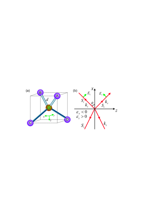
Figure 1: (color online) (a) Four possible orientations of NV centers in diamond Doherty2013 ; Zou2014 :
, , ,
. pm is the length of carbon
bond. The angle between any pair of the above four orientations is identically
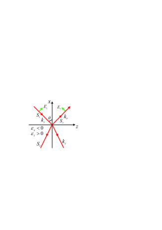
. (b) Negative refraction for
hyperbolic dispersion with and .
The TH mode is incident on the interface with electric field ,
wavevector , and Poynting vector . The angle
between the normal (-axis) and the incident field is . It
is reflected with electric field , wavevector ,
and Poynting vector . The Poynting and wavevector
of the transmitted wave are, respectively, and .
Model.––As schematically illustrated in Fig. 1(a),
an NV center is composed of a vacancy, e.g. site O, and a substitutional
nitrogen atom at one of its four possible neighboring sites, e.g.
site A, B, C and D. The electronic ground state is a spin-triplet
state with Hamiltonian Doherty2013 ; SuppMat
(1)
where GHz is the zero-field splitting of the
electronic ground state, is the Bohr magneton,
are respectively the components of the -factor of the electronic ground
state, is the magnetic field, and ()
are the spin-1 operators for the electron spin.
At room temperature, when there is no electric and strain fields,
the Hamiltonian of the electronic excited state is simplified as Doherty2013 ; SuppMat
(2)
where GHz is the zero-field splitting
of the electronic excited state,
is the -factor of the electronic spin of the excited state at
room temperature, MHz is the strain-related coupling.
As illustrated in Fig. 1(a), there are four possible
orientations for the NV centers in diamond Schirhagl2014 ; Wu2016 ; Doherty2013 ; Chen2017 ; Zou2014 ; SuppMat .
Since both Hamiltonians of the ground and excited states
are obviously dependent on the relative orientation
of the symmetry axis with respect to the magnetic field,
the energy spectra and thus the electromagnetic response of the NV
centers to the applied fields are different for the four possible
orientations.
Selection Rules of Optical Transitions.––According to Refs. Doherty2011 ; Maze2011 , there are four outer electrons
distributed in the , and levels, i.e. .
On account of the spin degree of freedom, the electronic ground states
are the triplet states labeled as SuppMat ,
, ,
where the superscript means configuration, the subscripts are
ordered as with being irreducible representation,
being row of irreducible representation, being total spin and being spin
projection along the symmetry axis of the NV center. The six first-excited
states, i.e. , are SuppMat ,
, ,
, ,
, where
and are degenerate under a magnetic field.
By comparing the ground and excited states,
there is one electron transiting from the
orbital to the orbital. Without spin-orbit coupling,
due to conservation of spin and total angular momentum Togan2010 ,
the non-zero transition matrix elements of the position vector are in the following
transitions
Maze2011 ; SuppMat ,
where and .
For the ground states, they can be formally diagonalized as ()
with eigenenergies . And for the excited states, they can
be formally diagonalized in two subsets according to their polarizations
as
and ()
with degenerate eigenenergies , where they share the same
coefficients due to the degeneracy.
According to Refs. Jackson1999 ; Landau1995 , the constitutive relation reads
,
where is the electric displacement,
is the electric permittivity of vacuum,
and are, respectively,
the relative permittivity tensor of diamond with and without NV centers.
The polarization density can be calculated using linear response theory Kubo1985 ; Fang2016 as
(3)
where is the Planck constant, is the density
of the NV centers, is the probability of the initial state
, is the frequency of the electric field ,
is the transition frequency of the th NV center between the initial state and the
final state , is the lifetime of the final state
, and is the transition matrix element of the electric
dipole of the th NV center between the initial and final states.
Note that in Eq. (3), and also in Eq. (S83).
In the above equation,
we did not explicitly discriminate the contributions from
and , as they only differ by the polarization
direction.
where and are the components of the
transition dipole of the th NV center. Clearly, there can be
nine possible negative permittivity components around the nine transition frequencies of the th NV center.
However, if a static magnetic field is applied along the -axis,
all transition frequencies would be correspondingly identical
for all four possible orientations Zou2014 .
Moreover, the relative permeability is not modified by the presence
of NV centers because the transition
can only be induced by the electric-dipole couplings to the electromagnetic
field.
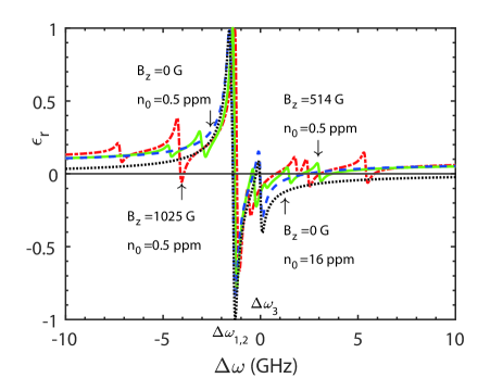
Figure 2: (color online) The frequency dependence of the electric permittivity
of diamond with NV centers for different values of the magnetic field
and density of NV centers : blue dashed line for G and ppm, green solid line for G and ppm, red dash-dotted line for G and
ppm, black dotted line for G and ppm. Other
parameters are D Lenef1996 ,
ns Acosta2011 , Fontanella1977 ,
and Young1992 , G.
The thin black line is just a guide to the eye.
In Fig. 2 we investigate the dependence of the permittivity
on the magnetic field and density of the NV centers.
Noticeably, two of the three components of the permittivity remain unchanged and
only one component is subtly modified by due to the symmetry
and the special choice of SuppMat .
As a special case, we plot the modified component of the permittivity
versus the frequency of the incident light for .
When the magnetic field is absent,
in the manifold of the electronic ground state,
are degenerate and there is an energy gap between them and .
For the manifold of the electronic excited state,
because are degenerate,
there would be level anti-crossing due to the strain-related coupling .
Since the electric-dipole induced transitions conserve the spin momentum Togan2010 ,
there could exist negative permittivity around three transition frequencies,
i.e. and GHz SuppMat .
However, in the blue dashed curve of Fig. 2,
we can only observe two negative dips around
the transition frequencies GHz and 0 GHz.
The first two dips merge into a single one as their widths, GHz, are
much larger than their separation, i.e. GHz.
As the frequency of the incident light grows,
the modified component of the permittivity eventually increases to become positive at GHz. Therefore, for and ppm,
the frequency window for demonstrating negative refraction is roughly (-1.46,2.37) GHz.
Because Eq. (S83) suggests negative permittivity to be around the transition frequencies, we hereafter explore the possibility of the negative refraction
beyond the above frequency domain by tuning magnetic field.
In the green solid curve of Fig. 2,
we plot the permittivity at the degenerate point of the excited states,
i.e., G. A new negative dip appears at GHz.
Interestingly, for the degenerate point of the ground states, i.e., G,
in addition to the other two at GHz
and GHz on the right,
there is a new negative dip at GHz
on the left hand side of ,
cf. red dash-dotted curve of Fig. 2.
Meanwhile, the depth of the main dip at has been reduced
as compared to the case when G.
The increasing magnetic field does not only modify the transition frequencies,
but also redistributes electric dipoles among the eigenstates. In this regard,
by tuning the magnetic field, we can switch on/off the negative refraction on demand.
In Fig. 2, there are only seven dips for the cases with G and G, because there are two sets of degenerate eigenstates as shown in SuppMat .
Furthermore, suggested by Eq. (S83),
the permittivity is also influenced by the density of the NV centers.
In the black dotted curve of Fig. 2,
this density is increased from ppm to ppm.
Compared to the blue dashed curve of Fig. 2,
the window of the negative refraction has been significantly broadened
because more NV centers can negatively respond to the applied magnetic field.
With this increased density, the negative dip at GHz
can be more profound for G.
Notice that in the numerical simulation we have not used the local field correction Jackson1999 ; Landau1995 ,
since the local field correction will not substantially change the center and
width of the negative refraction domain but will modify its magnitude Kastel2007-1 ; Kastel2007-2 ; Fang2016 ; SuppMat .
Therefore, we have demonstrated negative refraction by the normalized in Fig. 2.
Negative Refraction.––In Ref. Veselago1968 ,
it has been shown that for a double-negative metamaterial there
can be negative refraction. However, in the NV centers of diamond,
because the electric permittivity tensor possesses
two different components, it is natural to ask whether
negative refraction can exist. Below, we will demonstrate that
negative refraction can indeed occur for a TH incident mode SuppMat , cf.
Fig. 1(b).
According to Maxwell’s equations Jackson1999 ; Landau1995 ,
,
,
where both the current density and the charge density vanish,
is the permittivity of diamond with NV centers, and is the
permeability of pure diamond.
Assuming that the transmitted electric and magnetic fields are, respectively,
,
,
we have
(5)
where is the identity dyadic. For nontrivial
solutions, the dispersion relation for the extraordinary mode reads
(6)
assuming . Such a dispersion relation
for the extraordinary mode is hyperbolic or indefinite because .
According to the boundary condition Jackson1999 ,
the tangential components of the wavevector across the interface should
be equal, i.e.,
,
.
By inserting Eq. (S124) into Eq. (S116),
we obtain the relation between and as
.
By Maxwell equation, we have
(7)
The time-averaged Poynting vector reads Jackson1999
,
with the components being
,
,
because and . In order to transmit
energy from the interface into the medium, should be negative
and thus as . Together with Eq. (S124),
we have
(8)
where
.
Because , we have proven that for
a uniaxial crystal with hyperbolic dispersion, the negative
refraction exists for a TH incident field.
Experimental Feasibility.––For zero magnetic field,
the Hamiltonians of the electronic ground and excited states are further simplified as
and SuppMat ,
where we have omitted the strain-related coupling.
The transition electric dipole has been estimated as D Lenef1996 .
For simplicity, the orientations of all NV centers are assumed
to be along the -axis. Thus, all matrix
elements of the transition electric dipole are equal to
D.
Initially, the NV center is in the thermal state .
Therefore,
, and
(9)
where . The three
principal components of the relative permittivity are, respectively,
(10)
.
When the frequency of the incident field is ,
one principal component can be negative if
,
while the other principal components remain positive.
Because two carbon atoms occupy a volume ,
the minimum density of the NV centers to demonstrate negative refraction is
(11)
which is feasible in experimental fabrication, e.g. 16 ppm
Jarmola2012 . In addition, as proven in SuppMat ,
the negative component of permittivity appears in the -axis,
because of
and the symmetry of four possible orientations of the NV centers.
Conclusions.––In this work,
we proposed a new approach to realize hyperbolic metamaterial
using diamond with NV centers in the optical frequency regime.
Because of the long lifetime of the excited states of the NV centers,
this hyperbolic metamaterial manifests an intriguing window for negative refraction.
By varying the applied magnetic field to
tune the energy spectra of both ground and excited states,
the frequency of the negative refraction can be tuned in a wide range.
Note that it is difficult to fabricate classical metamaterials
working in optical-frequency domain,
because the sizes of the elements therein are sub-micron.
The NV-metamaterials proposed here solve this problem.
Because this NV-metamaterial can be used in subwavelength imaging,
spontaneous emission enhancement, heat transport and acoustics,
analogue cosmology, and lifetime engineering,
our proposal bridges the gap between NV centers and metamaterials.
Acknowledgements.
We thank stimulating discussion with Zhou Li and K. Y. Bliokh.
This work was supported by the MURI Center for Dynamic Magneto-Optics via the
AFOSR Award No. FA9550-14-1-0040, the Japan Society
for the Promotion of Science (KAKENHI), the IMPACT program of JST,
JSPS-RFBR grant No. 17-52-50023, CREST grant No. JPMJCR1676,
and RIKEN-AIST Challenge Research Fund. C.P.S. was supported by
NSFC under Grant No. 11421063 and No. 11534002, NSAF under Grant No. U1530401.
Q.A. was partially supported by NSFC under Grant No. 11505007.
References
(1) V. G. Veselago,
The electrodynamics of substances with simultaneously negative values of and ,
Sov. Phys. Uspekhi. 10, 509 (1968).
(2) J. B. Pendry,
Negative refraction makes a perfect lens,
Phys. Rev. Lett. 85, 3966 (2000).
(3) D. R. Smith, W. J. Padilla, D. C. Vier, S. C. Nemat-Nasser, and S. Schultz, Composite medium with simultaneously negative permeability and permittivity,
Phys. Rev. Lett. 84, 4184 (2000).
(4) K. Y. Bliokh, Y. P. Bliokh, V. Freilikher, S. Savel’ev, and F. Nori,
Colloquium: Unusual resonators: Plasmonics, metamaterials, and random media,
Rev. Mod. Phys. 80, 1201 (2008).
(5) Y. Shen and Q. Ai,
Optical properties of drug metabolites in latent fingermarks,
Sci. Rep. 6, 20336 (2016).
(6) Y. P. Bliokh, V. Freilikher, and F. Nori,
Ballistic charge transport in graphene and light propagation in periodic dielectric structures with metamaterials: A comparative study,
Phys. Rev. B 87, 245134 (2013).
(7) A. V. Kats, S. Savel’ev, V. A. Yampol’skii, and F. Nori,
Left-handed interfaces for electromagnetic surface waves,
Phys. Rev. Lett. 98, 073901 (2007).
(8) J. Yao, Z. Liu, Y. Liu, Y. Wang, C. Sun, G. Bartal, A. M. Stacy, and X. Zhang, Optical negative refraction in bulk metamaterials of nanowires,
Science 321, 930 (2008).
(9)Y. N. Fang, Y. Shen, Q. Ai, and C. P. Sun,
Negative refraction in Möbius molecules,
Phys. Rev. A 94, 043805 (2016).
(10) C. W. Chang, M. Liu, S. Nam, S. Zhang, Y. Liu, G. Bartal, and X. Zhang,
Optical Möbius symmetry in metamaterials,
Phys. Rev. Lett. 105, 235501 (2010).
(11) Y. Shen, H. Y. Ko, Q. Ai, S. M. Peng, and B. Y. Jin,
Molecular split-ring resonators based on metal string complexes,
J. Phys. Chem. C 118, 3766 (2014).
(12) A. L. Rakhmanov, V. A. Yampol’skii, J. A. Fan, F. Capasso, and F. Nori,
Layered superconductors as negative-refractive-index metamaterials,
Phys. Rev. B 81, 075101 (2010).
(13) A. Poddubny, I. Iorsh, P. Belov, and Y. Kivshar,
Hyperbolic metamaterials,
Nat. Photon. 7, 958 (2013).
(14) S. Jahani and Z. Jacob,
All-dielectric metamaterials,
Nat. Nanotechnol. 11, 23 (2016).
(15) D. R. Smith and D. Schurig,
Electromagnetic wave propagation in media with indefinite permittivity and permeability tensors, Phys. Rev. Lett. 90, 077405 (2003).
(16) P. A. Belov,
Backward waves and negative refraction in uniaxial dielectrics with negative dielectric permittivity along the anisotropy axis,
Microw. Opt. Technol. Lett. 37, 259 (2003).
(17) Z. Liu, H. Lee, Y. Xiong, C. Sun, and X. Zhang,
Far-field optical hyperlens magnifying sub-diffraction-limited objects,
Science 315, 1686 (2007).
(18) S. Ishii, A. V. Kildishev, E. Narimanov, V. M. Shalaev, and V. P. Drachev,
Sub-wavelength interference pattern from volume plasmon polaritons in a hyperbolic medium,
Las. Photon. Rev. 7, 265 (2013).
(19) Z. Jacob, I. Smolyaninov, and E. Narimanov,
Broadband Purcell effect: radiative decay engineering with metamaterials,
Appl. Phys. Lett. 100, 181105 (2012).
(20) S. A. Biehs, M. Tschikin, and P. Ben-Abdallah,
Hyperbolic metamaterials as an analog of a blackbody in the near field,
Phys. Rev. Lett. 109, 104301 (2012).
(21) J. Li, L. Fok, X. Yin, G. Bartal, and X. Zhang,
Experimental demonstration of an acoustic magnifying hyperlens,
Nature Mater. 8, 931 (2009).
(22) I. I. Smolyaninov and E. E. Narimanov,
Metric signature transitions in optical metamaterials,
Phys. Rev. Lett. 105, 067402 (2010).
(23) H. N. S. Krishnamoorthy, Z. Jacob, E. Narimanov, I. Kretzschmar, and V. M. Menon,
Topological transitions in metamaterials,
Science 336, 205 (2012).
(24) X. Yang, J. Yao, J. Rho, X. Yin, and X. Zhang,
Experimental realization of three-dimensional indefinite cavities at the nanoscale with anomalous scaling laws,
Nature Photon. 6, 450 (2012).
(25) R. Schirhagl, K. Chang, M. Loretz, and C. L. Degen,
Nitrogen-vacancy centers in diamond: Nanoscale sensors for physics and biology,
Annu. Rev. Phys. Chem. 65, 83 (2014).
(26) Y. Wu, F. Jelezko, M. B. Plenio, and T. Weil,
Diamond Quantum Devices in Biology,
Angew. Chem., Int. Ed. 55, 6586 (2016).
(27) M. W. Doherty, N. B. Manson, P. Delaney, F.
Jelezko, J. Wrachtrup, and L. C. L. Hollenberg,
The nitrogen-vacancy colour centre in diamond,
Phys. Rep. 528, 1 (2013).
(28) M. Chen, C. Meng, Q. Zhang, C. Duan, F. Shi, and J. F. Du,
Quantum metrology with single spins in diamond under ambient conditions,
Natl. Sci. Rev. in press (2017).
(29) J. Jeske, D. W. M. Lau, X. Vidal, L. P. McGuinness, P. Reineck, B. C. Johnson, M. W. Doherty, J. C. McCallum, S. Onoda, F. Jelezko, T. Ohshima, T. Volz, J. H. Cole, B. C. Gibson, and A. D. Greentree,
Stimulated emission from nitrogen-vacancy centres in diamond,
Nature Commun. 8, 14000 (2017).
(30) L. Jin, M. Pfender, N. Aslam, P. Neumann, S. Yang, J. Wrachtrup, and R.-B. Liu, Proposal for a room-temperature diamond maser,
Nature Commun. 6, 8251 (2015).
(31) M. P. Ledbetter, K. Jensen, R. Fischer, A. Jarmola, and D. Budker,
Gyroscopes based on nitrogen-vacancy centers in diamond,
Phys. Rev. A 86, 052116 (2012).
(32) B. B. Zhou, A. Baksic, H. Ribeiro, C. G. Yale, F. J. Heremans, P. C. Jerger, A. Auer, G. Burkard, A. A. Clerk, and D. D. Awschalom,
Accelerated quantum control using superadiabatic dynamics in a solid-state lambda system,
Nat. Phys. 13, 330 (2017).
(33) X. K. Song, Q. Ai, J. Qiu, and F. G. Deng,
Physically feasible three-level transitionless quantum driving with multiple Schrödinger dynamics,
Phys. Rev. A 93, 052324 (2016).
(34) F. Dolde, H. Fedder, M. W. Doherty, T. Nobauer, F. Rempp, G. Balasubramanian, T. Wolf, F. Reinhard, L. C. L. Hollenberg, F. Jelezko, and J. Wrachtrup,
Electric-field sensing using single diamond spins,
Nat. Phys. 7, 459 (2011).
(35) F. Dolde, M. W. Doherty, J. Michl, I. Jakobi, B. Naydenov, S. Pezzagna, J. Meijer, P. Neumann, F. Jelezko, N. B. Manson, and J. Wrachtrup,
Nanoscale Detection of a Single Fundamental Charge in Ambient Conditions Using the NV- Center in Diamond,
Phys. Rev. Lett. 112, 097603 (2014).
(36) J. R. Maze, P. L. Stanwix, J. S. Hodges, S. Hong, J. M. Taylor, P. Cappellaro, L. Jiang, M. V. G. Dutt, E. Togan, A. S. Zibrov, A. Yacoby, R. L. Walsworth, and M. D. Lukin,
Nanoscale magnetic sensing with an individual electronic spin in diamond,
Nature (London) 455, 644 (2008).
(37) G. Balasubramanian, I. Y. Chan, R. Kolesov, M. Al-Hmoud, J. Tisler, C. Shin, C. Kim, A. Wojcik, P. R. Hemmer, A. Krueger, T. Hanke, A. Leitenstorfer, R. Bratschitsch,
F. Jelezko, and J. Wrachtrup,
Nanoscale imaging magnetometry with diamond spins under ambient conditions,
Nature (London) 455, 648 (2008).
(38) L. S. Li, H. H. Li, L. L. Zhou, Z. S. Yang, and Q. Ai,
Measurement of weak static magnetic fields with nitrogen-vacancy color center,
Acta. Phys. Sin. 66, 230601 (2017).
(39) N. Zhao, J.-L. Hu, S.-W. Ho, T.-K. Wen, and R. B. Liu,
Atomic-scale magnetometry of distant nuclear spin clusters via nitrogen-vacancy spin in diamond,
Nat. Nanotechnol. 6, 242 (2011).
(40) M. S. Grinolds, S. Hong, P. Maletinsky, L. Luan, M. D. Lukin, R. L. Walsworth, and A. Yacoby,
Nanoscale magnetic imaging of a single electron spin under ambient conditions,
Nat. Phys. 9, 215 (2013).
(41) A. Cooper, E. Magesan, H. Yum, and P. Cappellaro,
Time-resolved magnetic sensing with electronic spins in diamond,
Nat. Commun. 5, 3141 (2014).
(42) F. Shi, Q. Zhang, P. Wang, H. Sun, J. Wang, X. Rong, M.
Chen, C. Ju, F. Reinhard, H. Chen, J. Wrachtrup, J. Wang, and J. F. Du,
Single-protein spin resonance spectroscopy under ambient conditions,
Science 347, 1135 (2015).
(43) S. J. DeVience, L. M. Pham, I. Lovchinsky, A. O. Sushkov, N. Bar-Gill, C. Belthangady, F. Casola, M. Corbett, H. Zhang, M. Lukin, H. Park, A. Yacoby, and R. L. Walsworth,
Nanoscale NMR spectroscopy and imaging of multiple nuclear species,
Nat. Nanotechnol. 10, 129 (2015).
(44) J. M. Boss, K. Chang, J. Armijo, K. Cujia, T. Rosskopf, J. R. Maze, and C. L. Degen,
One- and two-dimensional nuclear magnetic resonance spectroscopy with a diamond quantum sensor,
Phys. Rev. Lett. 116, 197601 (2016).
(45) H. B. Liu, M. B. Plenio, and J.-M. Cai,
Scheme for detection of single-molecule radical pair reaction using spin in diamond,
Phys. Rev. Lett. 118, 200402 (2017).
(46) Y.-Y. Wang, J. Qiu, Y.-Q. Chu, M. Zhang, J.-M. Cai, Q. Ai, and F.-G. Deng,
Dark state polarizing a nuclear spin in the vicinity of a nitrogen-vacancy center,
arXiv:1708.05467 (2017).
(47) G. Kucsko, P. C. Maurer, N. Y. Yao, M. Kubo, H. J. Noh, P. K. Lo, H. Park, and M. D. Lukin,
Nanometre-scale thermometry in a living cell,
Nature (London) 500, 54 (2013).
(48) D. M. Toyli, C. F. de las Casas, D. J. Christle, V. V.
Dobrovitski, and D. D. Awschalom,
Fluorescence thermometry enhanced by the quantum coherence of single spins in diamond,
Proc. Natl. Acad. Sci. U.S.A. 110, 8417 (2013).
(49) P. Neumann, I. Jakobi, F. Dolde, C. Burk, R. Reuter, G. Waldherr, J. Honert, T. Wolf, A. Brunner, J. H. Shim, D. Suter, H. Sumiya, J. Isoya, and J. Wrachtrup,
High-precision nanoscale temperature sensing using single defects in diamond,
Nano Lett. 13, 2738 (2013).
(50) Z.-L. Xiang, S. Ashhab, J. Q. You, and F. Nori,
Hybrid quantum circuits: Superconducting circuits interacting with other quantum systems, Rev. Mod. Phys. 85, 623 (2013).
(51) Z.-L. Xiang, X.-Y. Lü, T.-F. Li, J. Q. You, and F. Nori,
Hybrid quantum circuit consisting of a superconducting flux qubit coupled to a spin ensemble and a transmission-line resonator,
Phys. Rev. B 87, 144516 (2013).
(52) X.-Y. Lü, Z.-L. Xiang, W. Cui, J. Q. You, and F. Nori,
Quantum memory using a hybrid circuit with flux qubits and nitrogen-vacancy centers,
Phys. Rev. A 88, 012329 (2013).
(53) P.-B. Li, Z.-L. Xiang, P. Rabl, and F. Nori,
Hybrid quantum device with nitrogen-vacancy centers in diamond coupled to carbon nanotubes,
Phys. Rev. Lett. 117, 015502 (2016).
(54) A. M. Zagoskin, J. R. Johansson, S. Ashhab, and F. Nori,
Quantum information processing using frequency control of impurity spins in diamond,
Phys. Rev. B 76, 014122 (2007).
(56) L. J. Zou, D. Marcos, S. Diehl, S. Putz, J. Schmiedmayer, J. Majer, and P. Rabl, Implementation of the Dicke lattice model in hybrid quantum system arrays,
Phys. Rev. Lett. 113, 023603 (2014).
(57) J. J. Sakurai,
Modern Quantum Mechanics
(Addison-Wesley, Reading, MA, 1993).
(58) M. W. Doherty, N. B. Manson, P. Delaney, and L. C. L. Hollenberg,
The negatively charged nitrogen-vacancy centre in diamond: the electronic solution,
New J. Phys. 13, 025019 (2011).
(59) J. R. Maze, A. Gali, E. Togan, Y. Chu, A. Trifonov, E. Kaxiras, and M. D. Lukin, Properties of nitrogen-vacancy centers in diamond: the group theoretic approach,
New J. Phys. 13, 025025 (2011).
(60) E. Togan, Y. Chu, A. S. Trifonov, L. Jiang, J. Maze, L. Childress, M. V. G. Dutt, A. S. Sørensen, P. R. Hemmer, A. S. Zibrov, and M. D. Lukin,
Quantum entanglement between an optical photon and a solid-state spin qubit,
Nature (London) 466, 730 (2010).
(61) J. D. Jackson,
Classical Electrodynamics 3rd ed.,
(John Wiley, United States, 1999).
(62) L. D. Landau, E. M. Lifshitz, and L. P. Pitaevskii,
Electrodynamics of Continuous Media 2nd Ed.,
(Butterworth Heinmann, Oxford, 1995).
(63) R. Kubo, M. Toda, and N. Hashitsume,
Statistical Physics II Nonequilibrium Statistical Mechanics
(Springer-Verlag, Berlin Heidelberg, 1985).
(64) J. Kästel, M. Fleischhauer, S. F. Yelin, and R. L. Walsworth,
Tunable negative refraction without absorption via electromagnetically induced chirality,
Phys. Rev. Lett. 99, 073602 (2007).
(65) J. Kästel, M. Fleischhauer, and G. Juzeliūnas,
Local-field effects in magnetodielectric media: Negative refraction and absorption reduction,
Phys. Rev. A 76, 062509 (2007).
(66) A. Lenef, S. W. Brown, D. A. Redman, and S. C. Rand,
Electronic structure of the N-V center in diamond: Experiments,
Phys. Rev. B 53, 13427 (1996).
(67) V. M. Acosta,
Optical magnetometry with nitrogen-vacancy centers in diamond,
Ph.D. thesis, University of California, Berkeley, 2011.
(68) J. Fontanella, R. L. Johnston, J. H. Colwell, and C. Andeen,
Temperature and pressure variation of the refractive index of diamond,
Appl. Opt. 16, 2949 (1977).
(69) H. D. Young,
University Physics 7th Ed.,
(Addison Wesley, San Francisco, 1992).
(70) A. Jarmola, V. M. Acosta, K. Jensen, S. Chemerisov, and D. Budker,
Temperature- and magnetic-field-dependent longitudinal spin relaxation in nitrogen-vacancy ensembles in diamond,
Phys. Rev. Lett. 108, 197601 (2012).
Supplemental Material for “Tunable Quantum Hyperbolic Metamaterial
Using Nitrogen-Vacancy Centers in Diamond”
Qing Ai
Peng-Bo Li
Wei Qin
C. P. Sun
Franco Nori
SI Model
The Hamiltonian of an NV center in its electronic ground
state is Doherty2013
(S1)
Here, GHz is the zero-field splitting of the
electronic ground state; and
are the axial and non-axial components of hyperfine interaction tensor
of the electronic ground state; , , are the
spin operators of the nuclear spin; is the nuclear
electric quadruple parameter of the electronic ground state;
and are the Bohr magneton and nuclear magneton respectively;
and are respectively the -factors of electronic ground
state and nuclear spin;
D and D are the components
of electric dipole moment of the electronic ground state; ,
, and are the electric, magnetic and strain
fields respectively. The electron spin operators in the basis {,,}
are
(S2)
(S3)
(S4)
When there is no nuclear spin, electric and strain fields, the Hamiltonian
of the electronic ground state is simplified as
(S5)
At room temperature, the Hamiltonian of an NV center in the electronic
excited state is Doherty2013
(S6)
where GHz is the zero-field splitting
of the electronic excited state; and
are the axial and non-axial components
of hyperfine interaction tensor of the electronic excited state;
is the nuclear electric quadruple parameter of the electronic excited
state; is the -factor of electronic
spin of excited state at the room temperature;
D is the electric dipole moment of the excited state; MHz
is the strain-related coupling. When there is no nuclear spin, electric
and strain fields, the Hamiltonian of the electronic excited state
is simplified as
(S7)
SII Linear Response Theory
In order to simulate the electromagnetic response of the diamond with
NV centers in the presence of applied fields, we can employ the linear-response
theory Kubo1985 to calculate the electric permittivity and
magnetic permeability. When there is an electric field applied, the
NV center is polarized as
(S8)
where the Fourier transform of the time-dependent electric field with
amplitude and frequency
(S9)
is
(S10)
(S11)
Here, is the dipole-dipole correlation function,
(S12)
where the initial state of the NV center is
(S13)
with .
The electric dipole in the Heisenberg picture is
(S14)
where
(S15)
with () being the electronic ground (excited) state.
Because the Fourier transform of the electric field is
(S16)
the electric dipole of the NV center in the applied electric field is
(S17)
where
(S18)
where in the sum the final state should be different from the initial
state, i.e., ,
(S19)
with being phenomenologically introduced for the decay
of the excited state. Here,
is the transition energy between the initial state
and the final state . Therefore, the induced
electric dipole can be rewritten as
(S20)
Because of the rotating-wave approximation Ai2010 , the second
term of the above equation should be neglected, i.e.
(S21)
Assuming that all NV centers are identical, the polarization density
reads
(S22)
where is the number density of the NV centers in diamond.
SIII Lorentz Local Field Theory
According to Ref. Jackson1999 , in closely-packed molecules
the polarization of neighboring molecules gives rise to an internal
field at any molecule, in addition to the external
field . The internal field is
(S23)
where is the actual contribution from the
molecules close to the given molecule, and is the contribution
from those molecules treated in an average continuum. As proven in
Ref. Jackson1999 , in any crystal structure
due to symmetry, and thus .
By dipole approximation and assuming no net charge in the volume ,
the mean-field contribution is Jackson1999
(S24)
where Fontanella1977 is relative permittivity of diamond,
and the second term is summed over all induced molecular electric dipole moments
within the volume. Under the weak field approximation,
the induced dipole moment is
(S25)
where is generally a second-order tensor.
Since Jackson1999 ; Marques2008 ,
the polarization reads
As proven in Sec. SVII, in diamond with NV centers, is of the form
(S29)
where is the second part of Eq. (11) in the main text.
Therefore, the electric susceptibility is
(S30)
and the relative permittivity is
(S31)
The window of the negative refraction is determined by the two solutions to the equation
(S32)
which is not qualitatively different from the equation for the case
without the local field correction
(S33)
As a result,
both the center and width of the negative refraction domain are not
substantially modified by the Lorentz local field correction.
This is in consistent with the numerical results in Refs. Kastel2007-1 ; Kastel2007-2 ; Fang2016 .
SIV Selection Rules of Optical Transitions
According to Ref. Doherty2011 , there are four outer electrons
distributed in the , and levels, i.e., .
On account of the spin degree of freedom, the electronic ground states
can be written in the second quantization form,
with an overbar denoting spin-down, as
(S34)
(S35)
(S36)
where the superscript means configuration, the subscripts are
ordered as with being the irreducible representation,
being the row of irreducible representation, being the total
spin and being the spin projection along the symmetry axis
of the NV. The six first excited states, i.e., , are respectively
(S37)
(S38)
(S39)
(S40)
(S41)
(S42)
By comparing the above states, we notice that there is one electron
transiting from the orbital to the orbital. In the absence
of spin-orbital coupling, on account of conservation of spin and total
angular momentum Togan2010 , the following transitions are
allowed by the electric dipole coupling
(S43)
(S44)
(S45)
The non-zero transition matrix elements of the position vector
( unit vector along direction ) are listed as Maze2011
(S46)
(S47)
(S48)
Therefore, we have
(S49)
(S50)
(S51)
(S52)
(S53)
(S54)
(S55)
(S56)
(S57)
(S58)
(S59)
(S60)
To summarize, the selection rules for optical transitions are
(S61)
(S62)
(S63)
(S64)
(S65)
(S66)
where the label over the arrow indicates the polarization of the electric
field. In short,
(S67)
where and .
In addition, and
remain degenerate when applying a magnetic field.
For the electronic ground states, they can be formally diagonalized as
(S68)
with eigenenergies . For the electronic excited state,
they can be likewise diagonalized in two sets according to their polarizations as
(S69)
(S70)
with eigenenergies , where they share the same coefficients
due to the degeneracy.
where is the permittivity of the vacuum,
is the relative permittivity of diamond with NV centers,
is the applied electric field, is the relative permittivity
of pure diamond, and the polarization density can be calculated by
linear response theory Kubo1985 as
(S72)
Here,
is the matrix element of electric dipole of th NV center between
the initial state and final state ;
is the transition energy between the initial
state and the final state
of th NV center; and is the decay rate of the electronic
excited state. The summation is over all NV centers within
the volume , and is the frequency of the incident
light. In the above equation, we did not explicitly discriminate the
contributions from and
as they only differ by the polarization direction.
For the transition ,
note that
(S73)
(S74)
(S75)
(S76)
(S77)
(S78)
(S79)
(S80)
(S81)
Therefore, the induced dielectric polarization density can be written as
(S82)
As a result, the relative permittivity tensor is
(S83)
Clearly, there may be nine possible negative permittivities around
the nine transition frequencies .
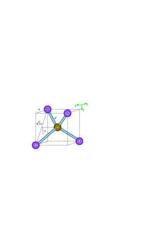
Figure S1: (color online) Four possible orientations of NV centers in diamond
Zou2014 ; Doherty2013 : , ,
, and .
pm is the length of carbon bond. The side length of the cube is .
The angle between any pair of the
above four orientations is .
As shown in Fig. S1, in diamond there are four
possible symmetry axes for the NV centers, i.e. ,
, , and
.
Here, can be obtained by rotating the -axis around the axis
by an angle ,
i.e.,
(S84)
where the rotation matrix around with
an angle is Sakurai1993
(S85)
And can be obtained by rotating the -axis around the axis
by an angle ,
i.e.,
(S86)
And can be obtained by rotating the -axis around the axis
by an angle ,
i.e.,
(S87)
And can be obtained by rotating the -axis around the axis
by an angle ,
i.e.,
(S88)
SV Quantum Switch of Negative Refraction and Normal Refraction
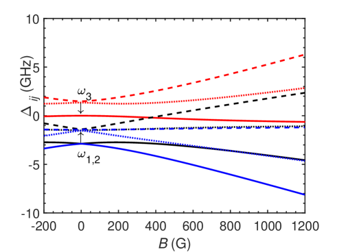
Figure S2: The transition frequencies
versus the magnetic field . The magnetic field is applied along
the -axis. This figure is identical for all four possible orientations
of the NV centers due to the special choice of .
As implied by Eq. (S83), the permittivity might be negative around the transition frequencies. In order to switch on/off the negative refraction,
we analyze the effect of the magnetic field on the transition frequencies.
As shown in Fig. S2,
there are generally nine transition frequencies ,
which can be subtly tuned by varying the magnetic field.
Below, we analyze the NV center at some specific magnetic fields:
(a) When the magnetic field is absent, the Hamiltonians of the electronic
ground state and excited state are respectively simplified as
(S89)
(S90)
The eigenstates of the electronic ground state are
(S91)
(S92)
(S93)
with eigenenergies
(S94)
(S95)
(S96)
The eigenstates of the electronic excited state are
(S97)
(S98)
(S99)
with eigenenergies
(S100)
(S101)
(S102)
Because the spin is conserved, the following optical transitions are
allowed
(S103)
(S104)
These correspond to five peaks around the transition frequencies ,
, , ,
and . Furthermore, because
and are degenerate,
and .
Since the separations between the latter four peaks are ,
which is, of the order of GHz, much smaller than the width of the peaks.
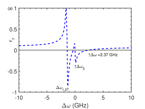
In Fig. S3, we plot the permittivity for different values
of the magnetic field and density of NV centers.
Therefore, we would only observe two dips for , as shown in Fig. S3(a).
Moreover, when the frequency is larger than GHz,
the permittivity becomes positive and thus negative refraction disappears.
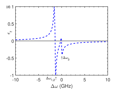
When the density is increased to ppm, cf. Fig. S3(d),
the two negative dips remains but the windows on the right is significantly broadened.
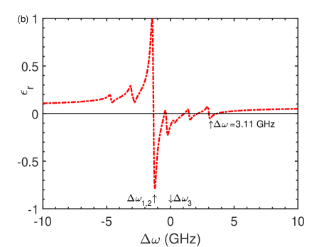
(b) When G, the electronic excited state is at the avoided
crossing point. Correspondingly, the Hamiltonians for the electronic ground and excited states are, respectively, given by
(S105)
(S106)
Since the couplings are comparable to the detunings,
the eigenstates in both manifolds effectively mix all three components, i.e.,
,
.
In this case, we would expect nine possible negative dips at nine transition frequencies.
In Fig. S3(b), we observe 7 dips
because the degeneracy has been partially broken
and there are still two sets of degenerate states.
As compared to Fig. S3(a),
there is an additional negative dip at GHz.
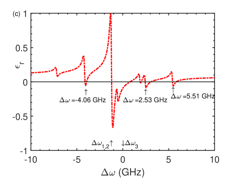
(c) When G, there are three additional negative dips at GHz,
GHz, and GHz beyond the domain GHz.
Figure S3: (color online) The frequency dependence of the electric permittivity
of diamond with NV centers for different values of the magnetic field
and density of NV centers : (a) G and ppm, (b) G and ppm, (c) G and ppm, (d) G and ppm. Other
parameters are D Lenef1996 ,
ns Acosta2011 , Fontanella1977 ,
and Young1992 , G.
The thin black line is just a guide to the eye.
SVI Negative Refraction at Interface
Figure S4: (color online) Negative refraction for hyperbolic dispersion with
and . The TH mode is incident on
the interface with electric field , wavevector ,
Poynting vector , and angle . It is reflected
with electric field , wavevector , and
Poynting vector . The Poynting vector, wavevector, electric
and magnetic fields of the transmitted wave are respectively ,
, , and .
By numerical simulation, we have shown that one principle component of the permittivity can be negative while the other principle components remain unchanged.
In this section, we will analytically prove that negative refraction can occur at the interface for a transverse magnetic (TH) mode, as shown in Fig. S4.
According to Maxwell’s equation Jackson1999 ; Landau1995 ,
(S107)
(S108)
(S109)
(S110)
where we have assumed and , is
the permittivity of diamond with NV centers, is the permeability
of vacuum and pure diamond.
Assuming that the electric and magnetic fields of the transmitted
wave are respectively
(S111)
(S112)
where and are respectively the wavevector
and frequency of the transmitted wave, we have
The time-averaged Poynting vector of the transmitted wave reads
(S129)
with the components being
(S130)
(S131)
because , and . In order to transmit
energy from the interface into the medium, should also be
negative, and thus as . Together
with Eq. (S124), we have
where and are, respectively, the permittivity
and permeability of diamond without NV centers, and
are respectively the electric and magnetic fields with frequency ,
the electric polarization and magnetization are respectively
(S136)
(S137)
Here is the matrix
element of electric dipole between the initial state
and the final state ; is the summation
over all NV centers within the volume . is
the transition frequency between the initial and final states;
is the homogeneous lifetime of all excited states; In the summation
the initial and final states should be different, . And
the system is initially in a state with density matrix .
When there is no magnetic field, the Hamiltonians of the electronic
ground and excited states are respectively simplified as
(S138)
(S139)
where we have dropped the interaction term in order to roughly estimate
the minimum density of NV centers in order to realize negative refraction.
The selection rule of optical transition is summarized as Acosta2011
,
where , both and are conserved. The transition
electric dipole has been experimentally estimated as D Lenef1996 .
In order to qualitatively estimate the minimum density of NV centers
for realizing negative refraction, without loss of generality, the
orientations of all NV centers are assumed to be along the -axis.
Thus, all of the matrix elements of the transition electric dipole
are equal
(S140)
For a specific NV center, should be replaced by the
orientation of its principle axis in the lab coordinate system, i.e.,
, , , and . Initially,
the NV center is in the state
(S141)
Therefore,
(S142)
(S143)
(S144)
where ns Acosta2011 ,
Fontanella1977 and Young1992
are the relative permittivity and permeability of the pure diamond.
For the diamond with NV centers, the electric displacement is
(S145)
and thus the tensor of relative permittivity is
(S146)
with three principal components being ,
and . In order to make , the critical density of the NV centers is
(S147)
Because as shown in Fig. S1 two carbon atoms occupy the volume
(S148)
the minimum density of the NV centers to achieve negative refraction is
(S149)
which is within the range of experimental fabrication, e.g. 16 ppm
Jarmola2012 .
For the NV center with the symmetry axis along ,
the principal axis of the negative permittivity is along .
For the NV center with the symmetry axis along ,
the principal axis of the negative permittivity is along .
For a medium with the above two orientations,
the principal axis of the negative permittivity is along the -axis.
In the same way, we can prove that for a medium with the other two orientations,
i.e. the symmetry axis along and ,
the principal axis of the negative permittivity is also along the -axis.
Therefore, for the diamond with NV centers along the four possible orientations,
the principal axis of the negative permittivity is along the -axis.
References
(1)
M. W. Doherty, N. B. Manson, P. Delaney, F. Jelezko, J. Wrachtrup, and L. C. L. Hollenberg,
The nitrogen-vacancy colour centre in diamond,
Phys. Rep. 528, 1 (2013).
(2)
R. Kubo, M. Toda, and N. Hashitsume,
Statistical Physics II Nonequilibrium Statistical Mechanics
(Springer-Verlag, Berlin Heidelberg, 1985).
(3)
Q. Ai, Y. Li, H. Zheng, and C. P. Sun,
Quantum anti-Zeno effect without rotating wave approximation,
Phys. Rev. A 81, 042116 (2010).
(4)
J. D. Jackson,
Classical Electrodynamics
3rd ed., (John Wiley, United States, 1999).
(5)
J. Fontanella, R. L. Johnston, J. H. Colwell, and C. Andeen,
Temperature and pressure variation of the refractive index of diamond,
Appl. Opt. 16, 2949 (1977).
(6)
R. Marqués, F. Martín, and M. Sorolla,
Metamaterials with Negative Parameters: Theory, Design and Microwave Applications
(John Wiley, New Jersey, 2008).
(7)
J. Kästel, M. Fleischhauer, S. F. Yelin, and R. L. Walsworth,
Tunable negative refraction without absorption via electromagnetically induced chirality,
Phys. Rev. Lett. 99, 073602 (2007).
(8)
J. Kästel, M. Fleischhauer, and G. Juzeliūnas,
Local-field effects in magnetodielectric media: Negative refraction and absorption reduction, Phys. Rev. A 76, 062509 (2007).
(9)
Y. N. Fang, Y. Shen, Q. Ai, and C. P. Sun,
Negative refraction in Möbius molecules,
Phys. Rev. A 94, 043805 (2016).
(10)
M. W. Doherty, N. B. Manson, P. Delaney, and L. C. L. Hollenberg,
The negatively charged nitrogen-vacancy centre in diamond: the electronic solution,
New J. Phys. 13, 025019 (2011).
(11)
E. Togan, Y. Chu, A. S. Trifonov, L. Jiang, J. Maze, L. Childress, M. V. G. Dutt, A. S. Sørensen, P. R. Hemmer, A. S. Zibrov, and M. D. Lukin,
Quantum entanglement between an optical photon and a solid-state spin qubit,
Nature 466, 730 (2010).
(12)
J. R. Maze, A. Gali, E. Togan, Y. Chu, A. Trifonov, E. Kaxiras, and M. D. Lukin,
Properties of nitrogen-vacancy centers in diamond: the group theoretic approach,
New J. Phys. 13, 025025 (2011).
(13)
L. D. Landau, E. M. Lifshitz, and L. P. Pitaevskii,
Electrodynamics of Continuous Media
2nd Ed., (Butterworth Heinmann, Oxford, 1995).
(14)
L. J. Zou, D. Marcos, S. Diehl, S. Putz, J. Schmiedmayer, J. Majer, and P. Rabl,
Implementation of the Dicke lattice model in hybrid quantum system arrays,
Phys. Rev. Lett. 113, 023603 (2014).
(15)
J. J. Sakurai,
Modern Quantum Mechanics
(Addison-Wesley, Reading, MA, 1993).
(16)
A. Lenef, S. W. Brown, D. A. Redman, and S. C. Rand,
Electronic structure of the N-V center in diamond: Experiments,
Phys. Rev. B 53, 13427 (1996).
(17)
V. M. Acosta,
Optical magnetometry with nitrogen-vacancy centers in diamond,
Ph.D. thesis, University of California, Berkeley, 2011.
(18)
H. D. Young,
University Physics
7th Ed., (Addison Wesley, San Francisco, 1992).
(19)
P. A. Belov,
Backward waves and negative refraction in uniaxial dielectrics with negative dielectric permittivity along the anisotropy axis,
Microw. Opt. Technol. Lett. 37, 259 (2003).
(20)
A. Jarmola, V. M. Acosta, K. Jensen, S. Chemerisov, and D. Budker,
Temperature- and magnetic-field-dependent longitudinal spin relaxation in nitrogen-vacancy ensembles in diamond,
Phys. Rev. Lett. 108, 197601 (2012).