Hierarchical environment-assisted dynamical speedup control

Abstract

We investigate the qubit in the hierarchical environment where the first level is just one lossy cavity while the second level is the $N$-coupled lossy cavities. In the weak coupling regime between the qubit and the first level environment, the dynamics crossovers from the original Markovian to the new non-Markovian and from no-speedup to speedup can be realized by controlling the hierarchical environment, i.e., manipulating the number of cavities or the coupling strength between two nearest-neighbor cavities in the second level environment. And we find that the coupling strength between two nearest-neighbor cavities and the number of cavities in the second level environment have the opposite effect on the non-Markovian dynamics and speedup evolution of the qubit. In addition, in the case of strong coupling between the qubit and the first level environment, we can be surprised to find that, compared with the original non-Markovian dynamics, the added second level environment cannot play a beneficial role on the speedup of the dynamics of the system.

I Introduction

With the rapid development of quantum information technology Nielsen ; Ladd , the dynamics of open systems has drawn more and more interest. Any open system inevitably takes environmental factor considerations into account Petruccione . The environment interacting with the open system is divided into memory effect and memoryless effect. In memoryless environment, the information flowed in a single way, i.e., the information only flows from the system to the environment results in Markovian dynamics. While the information flows in both directions, i.e., the information can backflow from the environment to the system and hence leads to the non-Markovian dynamics in the memory environment. Recently, the non-Markovian dynamics has been studied in theory Anjh ; Paz ; Wolf ; Tu ; Breuer ; Chruscinski ; Xiong ; Rivas ; Znidaric ; Zhangwm and in experiments Liubh ; Madsen ; Tang1 due to it plays a leading role in many real physical processes such as quantum state engineering, quantum control Xue ; D'Arrigo9 ; Bylicka and the quantum information processing Xiang ; Bennett ; Xu11 ; Aaronson ; Duan . And so far, the non-Markovian dynamics have proven to be motivated by the strong system-environment coupling, structure reservoirs, low temperatures, initial system-environment correlations and so on. Furthermore, to quantify non-Markovianity Caruso ; Huelga ; Laine ; Dajka ; Smirne ; Luo ; Luxm ; Chruscinski2 ; Lijg ; Alimm ; Piilo ; Lorenzo ; Plenio ; Mat ; Nguyen ; Smirne2 ; Franco ; Laine2 ; Liu4 ; Man1 ; Man2 , several measures Piilo ; Lorenzo ; Plenio have been proposed and the non-Markovian evolution process can absolutely be detected.

More importantly, some efforts has been recently devoted to investigating the role played by the non-Markovianity on the speed of evolution of quantum system Fan ; Deffner ; Sun ; Meng ; Zhangyj3 ; Xuzy ; Cimmarusti ; Anjh2 ; Zhangyj4 . For the damped Jaynes-Cummings model, in which a qubit resonantly interacts with a leaky single-mode cavity, reference Deffner has found that the non-Markovian effect could lead to speedup dynamics process in the strong system-environment coupling regime. And this theoretical result has been confirmed by increasing the system-environment coupling strength and the controllable number of atoms in the environment Cimmarusti . So far, some works usually consider the quantum system coupled to a single-layer environment. However, in realistic scenarios, the quantum system often inevitably couple to the multi-layer environments Hanson1 ; Hanson2 ; Pla ; Chekhovich ; Tyryshkin . Such as, the neighbor nitrogen impurities constitute the principle bath for a nitrogen-vacancy center, while the carbon-13 nuclear spins may also couple to them Hanson1 . In a quantum dot the electron spin may be affected strongly by the surrounding nuclei Hanson2 ; Chekhovich . A similar situation also occurs for a single-donor electron spin in silicon Pla ; Tyryshkin .

Recently, motivated by these facts, many efforts have been devoted to studying the effects of the multi-layer environments on the non-Markovian dynamics of an open system. The dynamics of a two-level atom has been studied in the presence of an overall environment composed of two layers Nguyen . In their model, the first layer is just a single lossy cavity while the second layer consists of a number of non-coupled lossy cavities. And the non-Markovian dynamics of the atom is affected by the coupling strength between the two layers and the number of cavities in the second layer. But in the lab, some actual physical systems (such as the couple cavity-array, the coupled spin chain and the coupled superconducting resonators) usually have been chosen to implement quantum computing and quantum simulation. So the influence of the coupling between two nearest-neighbor cavities in the second layer environment on the dynamics of the system can not be ignored.

So here we mainly study the dynamics of a qubit coupled with the two layer environments. By using the quantum speed limit (QSL) time Deffner ; 8 ; 08 to define the speedup evolutional process, we discuss that the influence of the coupling strength between two nearest-neighbor cavities and the number of cavities in the second-layer environment on the quantum evolutional speed of the qubit. As we all known, in the weak coupling regime between the qubit and the first-layer environment, the Markovian and no-speedup dynamics of the qubit would be followed when the second-layer environment has not been added. While in this paper, we elaborate how the non-Markovian speedup dynamics of the system can be obtained by controlling the coupling strength between two nearest-neighbor cavities and the number of cavities in the second-layer environment. Furthermore, we have also analyzed the influence of the parameters of the added second-layer environment on the non-Markovian speedup evolution of the qubit in the strong coupling regime between the qubit and the first-layer environment.

II Theoretical model

We consider that the total system consists of a qubit and the hierarchical environment where the cavity $m_{0}$ and its corresponding memoryless reservoir serve as the first-layer environment for the two-level atom and the other coupled cavities $m_{n}$ ($n=1$, 2, …, $N$) and memoryless reservoirs involved act as the second-layer environment, as depicted in Fig. 1.

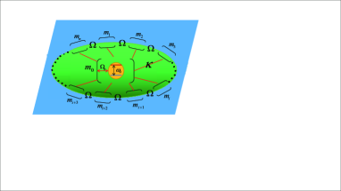
Figure 1: Schematic representation of the model. The stratified lossy cavities are selected as the controllable environment.

To be concrete, the qubit is coupled with strength $\Omega_{0}$ to a mode $m_{0}$ which decays to a memoryless reservoir with a lossy rate $\Gamma_{0}$ and then the mode $m_{0}$ is further coupled simultaneously with strengths $\kappa$ to modes $m_{n}$ which also decay to their respective memoryless reservoirs with rates $\Gamma_{n}=\Gamma$. Besides, the coupling strength between two nearest-neighbor cavities is $\Omega$ in the second-layer environment. The total Hamiltonian can be given by $H=H_{0}+H_{I}$, reads

$$H_{0} = \frac{\omega_{0}}{2}\sigma_{z}+\omega_{c}a^{{\dagger}}a+\sum_{n=1}^{N}\omega_{n}b^{{\dagger}}_{n}b_{n},$$

$$H_{I} = \Omega_{0}(\sigma_{+}a+\sigma_{-}a^{{\dagger}})+\sum_{n=1}^{N}\kappa(ab^{{\dagger}}_{n}+a^{{\dagger}}b_{n})$$ (1)

$$+ \sum_{\langle ij\rangle}\Omega(b^{{\dagger}}_{i}b_{j}+b^{{\dagger}}_{j}b_{i}).$$

In the above expressions, $\sigma_{z}=|1{\rangle}{\langle}1|-|0{\rangle}{\langle}0|$ is a pauli operator for the qubit with transition frequency $\omega_{0}$, $\sigma_{\pm}$ represent the raising and lowering operators of the qubit, and $a$ $(a^{{\dagger}})$ is the annihilation (creation) operator of mode $m_{0}$ with frequency $\omega_{c}$. Besides, $b^{{\dagger}}_{n}$ ($b_{n}$) is the creation (annihilation) operator of mode $m_{n}$ ($n=1$, 2, …, $N$) with frequency $\omega_{n}$. $\langle ij\rangle$ means the nearest neighbor cavities in the second-layer environment. Then the density operator $\rho(t)$ of the total system obeys the following master equation

$$\frac{d\rho}{dt}= - i[H,\rho]-\frac{\Gamma_{0}}{2}(a^{{\dagger}}a\rho-2a{\rho}a^{{\dagger}}+{\rho}a^{{\dagger}}a)$$ (2)

$$- \sum_{n=1}^{N}\frac{\Gamma}{2}(b^{{\dagger}}_{n}b_{n}\rho-2b_{n}{\rho}b^{{\dagger}}_{n}+{\rho}b^{{\dagger}}_{n}b_{n}),$$

For simplicity, we suppose that the atom is initially in its excited state $|1{\rangle}_{s}$, while all the cavities are in their ground states $|0...0{\rangle}_{m_{0}....m_{n}}$, i.e., the initial state of the total system is $\rho(0)=|10...0{\rangle}{\langle}10...0|$. Since there exist at most one excitation in the total system at a time, then $|\psi(t){\rangle}$ at time t can be written as $|\psi(t){\rangle}=g(t)|10...0{\rangle}+c_{0}(t)|01...0{\rangle}+c_{1}(t)|001...0{\rangle}+...+c_{n}(t)|000...1{\rangle}$, where $g(t)$, $c_{0}(t)$, $c_{1}(t)$, …, $c_{n}(t)$ correspond to probability amplitudes for the atom and modes $m_{0}$, $m_{1}$, …, $m_{n}$, respectively. Besides, the probability amplitudes $g(t)$, $c_{0}(t)$, $c_{1}(t)$, …, $c_{n}(t)$ of the system are governed by the Schr$\ddot{o}$dinger equation, from which we can obtain,

$$\begin{aligned} i\dot{g}(t)&=\Omega_{0}c_{0}(t),\\ i\dot{c_{0}}(t)&=(-\frac{i}{2}\Gamma_{0})c_{0}(t)+\Omega_{0}g(t)+\sum_{n=1}^{N}\kappa c_{n}(t),\\ i\sum_{n=1}^{N}\dot{c_{n}}(t)&=\sum_{n=1}^{N}(2\Omega-\frac{i}{2}\Gamma)c_{n}(t)+\kappa Nc_{0}(t).\end{aligned}$$ (3)

The solutions of the above equations can be obtained by means of Laplace transform method. For convenience, we express the dynamics of the qubit by the reduced density matrix in the system’s bases $\{|1{\rangle}_{s}$, $|0{\rangle}_{s}\}$ as

$$\rho(t)=\left(\begin{array}[]{cc}\rho_{11}(0)|g(t)|^{2}&\rho_{01}(0)g(t)^{\ast}\\ \rho_{10}(0)g(t)&\rho_{00}(0)+\rho_{11}(0)(1-|g(t)|^{2})\\ \end{array}\right)$$ (4)

where $\rho_{11}(0)=1$, $\rho_{00}(0)=\rho_{01}(0)=\rho_{10}(0)=0$. Then in our scheme, it needs to be emphasized that we mainly focus on the dynamical behavior of the atomic system can be modified by the second-layer controllable environment in the weak qubit-$m_{0}$ coupling regime ($\Omega_{0}<\Gamma_{0}/4$) and the strong qubit-$m_{0}$ couple regime ($\Omega_{0}>\Gamma_{0}/4$).

III Non-Markovian dynamics control

In order to further illustrate the roles of the parameters in the considered second-layer environment, i.e., the number $N$ of cavities and the coupling strength $\Omega$ between two nearest-neighbor cavities, in what follows we would describe how to tune the controllable second-layer environment from Markovian to non-Markovian by manipulating $N$ and $\Omega$. A general measure $\mathbf{N}(\Phi)$ for non-Markovianity, which can be used to distinguish the Markovian dynamics and the non-Markovian dynamics of the quantum system, has been defined by Breuer $et$ $al$. Breuer . For a quantum process $\Phi(t)$, $\rho^{s}(t)=\Phi(t)\rho^{s}(0)$, with $\rho^{s}(0)$ and $\rho^{s}(t)$ denote the density operators at time $t=0$ and at any time $t>0$ of the quantum system, respectively, then the non-Markovianity $\mathbf{N}(\Phi)$ is quantified by $\mathbf{N}(\Phi)=\max_{\rho^{s}_{1,2}(0)}\int_{\sigma>0}dt\sigma[t,\rho^{s}_{1,2}(0)],$ with $\sigma[t,\rho^{s}_{1,2}(0)]=\frac{d}{dt}\mathcal{D}(\rho^{s}_{1}(t),\rho^{s}_{2}(t))$ is the rate of change of the trace distance. The trace distance $\mathcal{D}$ describing the distinguishability between the two states is defined as Nielsen $\mathcal{D}(\rho^{s}_{1},\rho^{s}_{2})=\frac{1}{2}\|\rho^{s}_{1}-\rho^{s}_{2}\|,$ where $\|M\|=\sqrt{M^{{\dagger}}M}$ and $0{\leq}\mathcal{D}\leq 1$. And $\sigma[t,\rho^{s}_{1,2}(0)]\leq 0$ corresponds to all dynamical semigroups and all time-dependent Markovian processes. While a process is non-Markovian if there exists a pair of initial states and at certain time $t$ such that $\sigma[t,\rho^{s}_{1,2}(0)]>0$. We should take the maximum over all initial states $\rho^{s}_{1,2}(0)$ to calculate the non-Markovianity. In Refs. Breuer ; Lijg , by drawing a sufficiently large sample of random pairs of initial states, it is proved that the optimal state pair of the initial states can be chosen as $\rho^{s}_{1}(0)=(|0\rangle_{s}+|1\rangle_{s})/\sqrt{2}$ and $\rho^{s}_{2}(0)=(|0\rangle_{s}-|1\rangle_{s})/\sqrt{2}$. Here, for this optimal state pair, the rate of change of the trace distance can be acquired $\sigma[t,\rho^{s}_{1,2}(0)]=\partial_{t}|g(t)|^{2}$. Then the non-Markovianity of the quantum system dynamics process from $\rho^{s}(0)$ to $\rho^{s}(t)$ can be calculated by $\mathbf{N}(\Phi)=\int^{t}_{0}(\partial_{t}|g(t)|^{2})|_{>0}dt$.

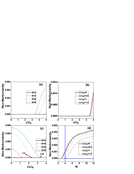
Figure 2: (Color online) (a), (b) The non-Markovianity $\mathbf{N}(\Phi)$ of the atomic system dynamics process from $\rho^{s}_{0}=|1\rangle_{s}{\langle}1|$ to $\rho^{s}_{\tau}$ as a function of the coupling strength $\kappa$ between the first-layer environment and the second-layer environment in the weak qubit-$m_{0}$ coupling regime $\Gamma_{0}=5\Omega_{0}$. (c) and (d) The non-Markovianity $\mathbf{N}(\Phi)$ of the atomic system dynamics process from $\rho^{s}_{0}=|1\rangle_{s}{\langle}1|$ to $\rho^{s}_{\tau}$ as a function of the coupling strength $\Omega$ between two nearest-neighbor cavities and the number of cavities $N$ in the weak qubit-$m_{0}$ coupling regime $\Gamma_{0}=5\Omega_{0}$. The other parameters are: (a) $\Omega=\Omega_{0}$, $\Gamma=5\Omega_{0}$, $\tau=3$; (b) $N=4$, $\Gamma=5\Omega_{0}$, $\tau=3$; (c) and (d) $\kappa=5\Omega_{0}$, $\Gamma=5\Omega_{0}$, $\tau=3$.

As we all know, if there are no any other-layer environment, the system’s dynamics mainly depends on the parameters $\Omega_{0}$ and $\Gamma_{0}$ in such a way that $\Gamma_{0}>4\Omega_{0}$ ($\Gamma_{0}<4\Omega_{0}$), identified as the weak (strong) coupling regime, leads to Markovian (non-Markovian) dynamics. Then in the case of adding the second-layer environment, the non-Markovianity $\mathbf{N}(\Phi)$ of the atomic dynamics process in the weak qubit-$m_{0}$ coupling regime from $\rho^{s}_{0}$ to $\rho^{s}_{\tau}$ as function of the controllable second-layer environment parameters ($\kappa$, $\Omega$, $N$) with the actual evolution time $\tau=3$, has been plotted in Fig. 2. Firstly, by fixing $\Omega=\Omega_{0}$, $\Gamma_{0}=5\Omega_{0}$ in the Fig. $2(a)$, in the case $N=2$, the non-Markovian dynamics of the atomic system cannot be obtained by tuning the $m_{0}-m_{n}$ coupling strength $\kappa$. However, if the lossy cavity $m_{0}$ simultaneously interacts the second-layer environment constituted by more than the number of cavities $N=2$, then a remarkable dynamical crossover from Markovian behavior to non-Markovian behavior can occur at a certain critical coupling strength $\kappa_{c1}$. When $\kappa<\kappa_{c1}$, the dynamics process abides by Markovian behavior, and then the non-Markovianity increase monotonically with increasing $\kappa$. Similarly, in the case $\Omega=1.5\Omega_{0}$ in the Fig. $2(b)$, no matter how to adjust the parameter $\kappa$, the dynamics process is Markovian. However, the non-Markovian dynamics can be triggered at a threshold $\kappa_{c2}$ by decreasing the coupling strength $\Omega$ between two nearest-neighbor cavities, such as, $\Omega=0,0.5\Omega_{0},\Omega_{0}$. And it is clear to point that, when $\kappa<\kappa_{c2}$ the dynamics process is Markovian, and the non-Markovianity increases with increasing $\kappa$ in the case $\kappa>\kappa_{c2}$. Finally, in the weak qubit-$m_{0}$ coupling regime, it needs to be emphasized that, the larger the value $\kappa$ ($N$), the smaller value $\Omega$ should be requested to trigger the non-Markovianity of the system.

In the following, in order to more intuitively explain the effect of parameters $\Omega$ and $N$ on the non-Markovianity of the system in weak qubit-$m_{0}$ coupling regime, we firstly fix $\kappa=5\Omega_{0}$ larger than the above critical value $\kappa_{c1}$ or $\kappa_{c2}$ in the Figs. $2(c)$ and $2(d)$. It is worth noting that, the dynamical crossover from Markovian behavior to non-Markovian behavior for the atomic dynamics process ($\rho^{s}_{0}$ to $\rho^{s}_{\tau}$) could appear by tuning $\Omega$, $N$. When the value $N$ is confirmed in Fig. 2(c), in the case $\Omega>\Omega_{c}$ ($\Omega_{c}$ means the critical value of $\Omega$), the dynamics process always abides by Markovian behavior, but the non-Markovianity increases monotonically with reducing $\Omega$ when $\Omega<\Omega_{c}$. That means the increasing of the coupling strength $\Omega$ in the second-layer environment could suppress the non-Markovian dynamics of the atomic system. Moreover, the larger the value $N$, the larger the critical value $\Omega_{c}$ should be acquired. Take the cases in Fig. $2(c)$: when $N=6$, we find the critical value $\Omega_{c1}=2.39\Omega_{0}$. While in the case $N=8$, $\Omega_{c2}=3.25\Omega_{0}$ should be given. Furthermore, it is interesting to find that, by fixing $\Omega=1.5\Omega_{0}$ in the Fig. $2(d)$, the dynamics process abides by Markovian up to $N=3$, but becomes non-Markovian starting from $N=4$. However, the non-Markovian dynamics is induced from $N=3$ by decreasing the coupling strength $\Omega$, say, $\Omega=0,0.5\Omega_{0},\Omega_{0}$. In general, it is worth noting that a larger $\Omega$ ($N$) could lead to a larger critical $N$ ($\Omega$). Finally, in the weak qubit-$m_{0}$ coupling regime, we find that the non-Markovian dynamic can be triggered by manipulating the added second-layer environment parameters.

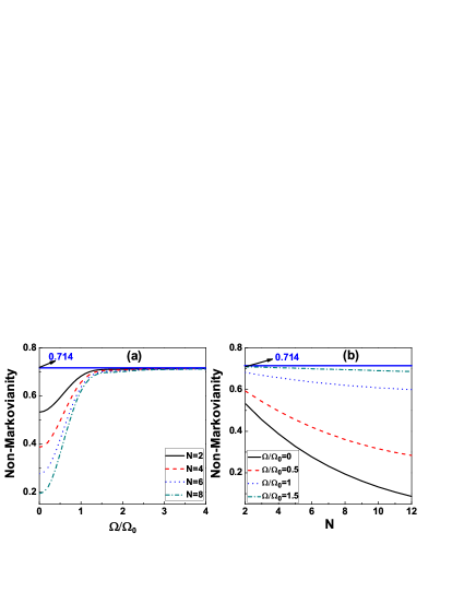
Figure 3: (Color online) (a), (b) The non-Markovianity $\mathbf{N}(\Phi)$ of the atomic system dynamics process from $\rho^{s}_{0}=|1\rangle_{s}{\langle}1|$ to $\rho^{s}_{\tau}$ as a function of the coupling strength $\Omega$ between two nearest-neighbor cavities and the number of cavities $N$ in the strong qubit-$m_{0}$ coupling regime $\Gamma_{0}=0.2\Omega_{0}$. The parameters are: $\Gamma=0.2\Omega_{0}$, $\kappa=0.2\Omega_{0}$, $\tau=3$.

It is well known that in the absence of the second-layer environment, the dynamics process of the system is non-Markovian in the strong qubit-$m_{0}$ coupling regime. Next, Figs. $3(a)$ and $3(b)$ show the non-Markovianity $\mathbf{N}(\Phi)$ of the atomic dynamics process from $\rho^{s}_{0}$ to $\rho^{s}_{\tau}$ is affected by the parameters $\Omega$ or $N$ with the actual evolution time $\tau=3$ when the strong qubit-$m_{0}$ coupling satisfied $\Gamma_{0}=0.2\Omega_{0}$. The blue solid line $N(\Phi)=0.714$ in Fig. 3 means the value of non-Markovianity without the second-layer environment. By fixing $N$ in Fig. 3(a), the non-Markovianity increases and tends to the original non-Markovianity $N(\Phi)=0.714$ of the atomic system with increasing the coupling strength $\Omega$ between two nearest-neighbor cavities, implying the coupling strength $\Omega$ between the two nearest-neighbors in the second-level environment can promote the non-Markovian dynamics of the system. Furthermore, by fixing $\Omega$ in the Fig. 3(b), the non-Markovianity of the system increases with decreasing the number of cavities $N$ in the second-layer environment. And it is clear to find that, irrespective of $\Omega$, $N$, the non-Markovianity is always below the original non-Markovianity ($0.714$) of the system. That is to say, compared with the previous non-Markovian dynamics in the strong qubit-$m_{0}$ coupling regime, the added second-layer environment can not contribute to promote the non-Markovianity of the system. Besides, in stark contrast, when the parameters $N$ and $\Omega$ make it possible to trigger the non-Markovianity of the system under the weak qubit-$m_{0}$ coupling regime, the non-Markovianity of the system is weakened under the strong qubit-$m_{0}$ coupling regime at this time. That is to say, in the cases of weak qubit-$m_{0}$ coupling regime and strong qubit-$m_{0}$ coupling regime, the second-layer environment parameters $\Omega$ and $N$ have different effects on the non-Markovian dynamics of the system. This is a newly noticed phenomenon.

IV Quantum speedup of the atomic dynamics

Recently, the relationship between non-Markovianity and the QSL times has been given by $\frac{\tau_{QSL}}{\tau}=\frac{1-|g(t)|^{2}}{2\mathbf{N}(\Phi)+1-|g(t)|^{2}}$ Xuzy ; Zhangyj4 . So the same critical values ($\Omega$, $N$) can be obtained from the Markovian process to the non-Markovian process and from no-speedup of quantum evolution to speedup. And the above equation implies that the stronger the non-Markovianity, the lower the QSL times (the quantum speedup evolution would occur). Then in our investigated model, it is easily to find that the purpose of accelerating the evolution of the quantum system can also be achieved by the controllable non-Markovianity discussed aboved. Obviously, in this section, we mainly focus on how the coupling strength $\Omega$ and the number of cavities $N$ to accelerate the evolution of quantum system. In order to characterize how fast the quantum system evolves, here we use the definition of the QSL time for an open quantum system, which can be helpful to analyze the maximal speed of evolution of an open system. The QSL time between an initial state $\rho^{s}(0)=|\phi_{0}\rangle\langle\phi_{0}|$ and its target state $\rho^{s}(\tau)$ for open system is defined by Deffner $\tau_{QSL}=\sin^{2}[\mathbf{B}(\rho^{s}(0),\rho^{s}(\tau))]/\Lambda^{\infty}_{\tau}$, where $\mathbf{B}(\rho^{s}(0),\rho^{s}(\tau))=\arccos\sqrt{\langle\phi_{0}|\rho^{s}(\tau)|\phi_{0}\rangle}$ denotes the Bures angle between the initial and target states of the system, and $\Lambda^{\infty}_{\tau}=\tau^{-1}\int^{\tau}_{0}\|\dot{\rho}^{s}(t)\|_{\infty}dt$ with the operator norm $\|\dot{\rho}^{s}(t)\|_{\infty}$ equaling to the largest singular value of $\dot{\rho}^{s}(t)$. When the ratio between the QSL time and the actual evolution time equals one, i.e., $\tau_{QSL}/\tau=1$, the quantum system evolution is already along the fastest path and possesses no potential capacity for further quantum speedup. While for the case $\tau_{QSL}/\tau<1$, the speedup evolution of the quantum system may occur and the much shorter $\tau_{QSL}/\tau$, the greater the capacity for potential speedup will be.

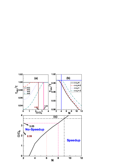
Figure 4: (Color online) (a), (b) The QSL time for the atomic system dynamic process with $\Gamma_{0}=5\Omega_{0}$ in the weak qubit-$m_{0}$ coupling regime as a function of the coupling strength $\Omega$ and the number of cavities $N$ in the second-layer environment. (c)Phase diagram of QSL time in the $\Omega$-$N$ plane with $\Gamma_{0}=5\Omega_{0}$ in the weak qubit-$m_{0}$ coupling regime. The parameters are: $\Gamma=5\Omega_{0}$, $\kappa=5\Omega_{0}$.

Then, for the weak qubit-$m_{0}$ coupling regime, the variations of the QSL time $\tau_{QSL}/\tau$ with respect to $\Omega$ and $N$ are plotted in Fig. 4. It is clearly found that, in the Fig. $4(a)$, the quantum system has no potential capacity for the further quantum speedup until the number of cavities in the second-layer environment above $N=2$. In order to verify, in the case $N=2$ in Fig. $4(a)$, the no-speedup evolution ($\tau_{QSL}/\tau=1$) could be followed, and the speedup evolution ($\tau_{QSL}/\tau<1$) would occur when the coupling strength $\Omega$ is less than a certain critical coupling strength $\Omega_{c}$ in the cases $N=4$, $6$, $8$. In addition, it is worth noting that, the larger the value $N$, the larger the critical value $\Omega_{c}$ may be requested. As shown in the Fig. $4(a)$, when $N=6$, $\Omega_{c1}=2.39\Omega_{0}$. While $N=8$, $\Omega_{c2}=3.25\Omega_{0}$. That is same as the above discussion for the non-Markovianity. As for Fig. 4(b), by fixing $\Omega=1.5\Omega_{0}$, the speedup evolution may occur when the number of cavities $N>4$ in the second-layer environment. However, by considering $\Omega=0$, $0.5\Omega_{0}$, $\Omega_{0}$, the speedup evolution can be induced by $N>3$. So we get an interesting conclusion that the coupling strength $\Omega$ and the number of cavities $N$ in the second-layer environment have the opposite effect on the speedup quantum evolution of the atomic system, namely, the quantum evolution would speedup by decreasing $\Omega$ or increasing $N$. So in the weak qubit-$m_{0}$ coupling regime, the purpose of accelerating evolution can be achieved by controlling the hierarchical environment.

In order to clear the region of parameters in which the speedup dynamics of the system can be eventuated in the weak qubit-$m_{0}$ coupling regime, Fig. $4(c)$ describes the $\Omega-N$ phase diagrams. And the transition points from no-speedup to speedup regime could be acquired. Take the cases in Fig. $4(c)$: when the value $N=6$, $8$ are fixed, the corresponding critical values of $\Omega$ have also been respectively given by $\Omega_{c1}=2.39\Omega_{0}$ and $\Omega_{c2}=3.25\Omega_{0}$. Still further, by fixing $N$, when $\Omega<\Omega_{c}$, the quantum speedup evolution would occur and then remain no-speedup with the increasing $\Omega$. It is worth noting that the number of the cavities in the second-layer environment must be more than $2$. The smaller $\Omega$ and the larger $N$ should be manipulated to drive the purpose of speedup evolution of the quantum system in the weak qubit-$m_{0}$ coupling regime.

For the strong qubit-$m_{0}$ coupling regime, by fixing $\Gamma_{0}=0.2\Omega_{0}$ and $\kappa=0.2\Omega_{0}$, we plot the variations of the QSL time $\tau_{QSL}/\tau$ with respect to $\Omega$ and $N$ in Fig. 5. Then this blue solid line indicates that when no adding the second-layer environment, the ratio value of $\tau_{QSL}/\tau$ is equal to $0.166$. Clearly shown in Fig. 5, the value of $\tau_{QSL}/\tau$ decreases and tends to 0.166 as the increasing of $\Omega$ in the Fig. $5(a)$. That is to say, the increasing of $\Omega$ can accelerate the evolution of the system in our two-layer environments. Besides, by fixing $\Omega$ in the Fig. $5(b)$, the QSL time always increase as the increasing of the number of cavities $N$. However, regardless of how to tune parameters $N$ or $\Omega$ in the Fig. 5, the QSL time is always larger than 0.166. That is to say, although $N$ or $\Omega$ can affect the QSL time of the dynamics process of the system in the strong qubit-$m_{0}$ coupling regime, the added second level environment cannot play a beneficial role on the speedup of the dynamics of the system.

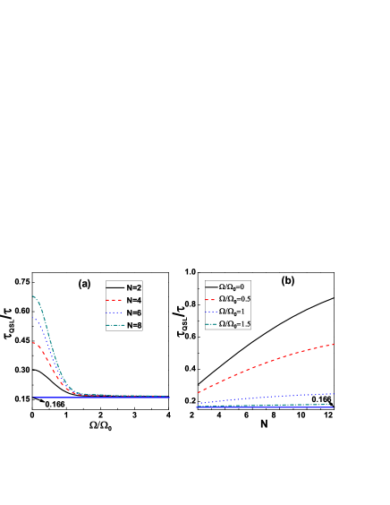
Figure 5: (Color online) (a), (b) The QSL time for the atomic system dynamic process with $\Gamma_{0}=0.2\Omega_{0}$ in the strong qubit-$m_{0}$ coupling regime as a function of the coulping-strength $\Omega$ and the number of cavities $N$. The parameters are: $\Gamma=0.2\Omega_{0}$, $\kappa=0.2\Omega_{0}$.

V Conclusion

In conclusion, we have investigated the dynamics of the qubit in a controllable hierarchical environment where the first-layer environment is a lossy cavity $m_{0}$ and the second-layer environment are the other coupled lossy cavities. Some interesting phenomena are observed. On the one hand, by controlling the number of cavities $N$ and the coupling strength $\Omega$ between two nearest-neighbor cavities in the second-layer, two dynamical crossovers of the quantum system, from the original Markovian to the new non-Markovian dynamics and from no-speedup evolution to speed evolution, have been achieved in the weak qubit-$m_{0}$ coupling regime. And it is worth noting that the coupling strength $\Omega$ and the number of cavities $N$ have the opposite effect on the non-Markovian dynamics and speedup evolution of the atomic system in the weak qubit-$m_{0}$ coupling regime. Furthermore, the transitions from no-speedup phase to speedup phase and from Markovian to non-Markovian effect for the system, have been demonstrated in our work. On the other hand, by considering the strong qubit-$m_{0}$ coupling regime, compared with the original non-Markovian dynamics without the second-layer environment, the added second-layer environment can not promote the speedup evolution of the system. And for the weak qubit-$m_{0}$ coupling regime and strong qubit-$m_{0}$ coupling regime, the second-layer environment parameters $\Omega$ and $N$ have different effects on the non-Markovian speedup dynamics of the system. Our hierarchical environment-assisted non-Markovian speedup dynamics control is essential to most purposes of quantum optimal control.

VI Acknowledgements

This work is supported by the National Natural Science Foundation of China (11647171, 61675115, 91536108), MOST of China (2016YFA0302104, 2016YFA0300600), and the Foundation of Chinese Academy of Sciences (XDB01010000, XDB21030300).

References

- (1) M. Nielsen and I. Chuang, Quantum Optics (Cambridge University Press, Cambridge, 2000).
- (2) T. D. Ladd, F. Jelezko, R. Laflamme, Y. Nakamura, C. Monroe, and J. L. O’Brien, Nature 464, 45 (2010).
- (3) H. P. Breuer and F. Petruccione, Theory of Open Quantum Systems (Oxford University Press, New York, 2002).
- (4) J. H. An, and W. M. Zhang, Phys. Rev. A 76, 042127 (2007).
- (5) J. P. Paz, and A. J. Roncaglia, Phys. Rev. Lett. 100, 220401 (2008); Phys. Rev. A 79, 032102 (2009).
- (6) M. M. Wolf, J. Eisert, T. S. Cubitt, and J. I. Cirac, Phys. Rev. Lett. 101, 150402 (2008).
- (7) M. W. Y. Tu, and W. M. Zhang, Phys. Rev. B 78, 235311 (2008).
- (8) H. P. Breuer, E. M. Laine, and J. Piilo, Phys. Rev. Lett. 103, 210401 (2009); E. M. Laine, J. Piilo, and H. P. Breuer, Phys. Rev. A 81, 062115 (2010).
- (9) D. Chruscinski, and A. Kossakowski, Phys. Rev. Lett. 104, 070406 (2010); D. Chruscinski, A. Kossakowski, and A. Rivas, Phys. Rev. A 83, 052128 (2011).
- (10) H. N. Xiong, W. M. Zhang, X. Wang, and M. H. Wu, Phys. Rev. A 82, 012105 (2010); C. U. Lei, and W. M. Zhang, Phys. Rev. A 84, 052116 (2011).
- (11) A. Rivas, S. F. Huelga, and M.B. Plenio, Phys. Rev. Lett. 105, 050403 (2010).
- (12) M. Znidaric, C. Pineda, and I. Garcia-Mata, Phys. Rev. Lett. 107, 080404 (2011).
- (13) W. M. Zhang, P. Y. Lo, H. N. Xiong, M. W. Y. Tu, and F. Nori, Phys. Rev. Lett. 109, 170402 (2012).
- (14) B. H. Liu, L. Li, Y. F. Huang, C. F. Li, G. C. Guo, E. M. Laine, H. P. Breuer, and J. Piilo, Nat. Phys. 7, 931 (2011).
- (15) K. H. Madsen, S. Ates, T. Lund-Hansen, A. Loffler, S. Reitzenstein, A. Forchel, and P. Lodahl, Phys. Rev. Lett. 106, 233601 (2011).
- (16) J. S. Tang, C. F. Li, Y. L. Li, X. B. Zou, G. C. Guo, H. P. Breuer, E. M. Laine, and J. Piilo, Europhys. Lett. 97, 10002 (2012).
- (17) S. B. Xue, R. B. Wu, W. M. Zhang, J. Zhang, C. W. Li, and T. J. Tarn, Phys. Rev. A 86, 052304 (2012).
- (18) A. D’Arrigo, R. Lo. Franco, G. Benenti, E. Paladino, and G. Falci, Ann. Phys. 350, 211 (2014).
- (19) B. Bylicka, D. Chruscinski, and S. Maniscalco, Sci. Rep. 4, 5720 (2014).
- (20) Z. L. Xiang, S. Ashhab, J. You, and F. Nori, Rev. Mod. Phys. 85, 623 (2013).
- (21) C. H. Bennett, and D. P. Divincenzo, Nature 404, 247-255 (2000).
- (22) J. S. Xu, K. Sun, C. F. Li, X. Y. Xu, G. C. Guo, E. Andersson, R. Lo Franco, and G. Compagno, Nat. Commun. 4, 2851 (2013).
- (23) B. Aaronson, R. Lo Franco, and G. Adesso, Phys. Rev. A 88, 012120 (2013).
- (24) L. M. Duan, M. D. Lukin, J. I. Cirac, and P. Zoller, Nature 414, 413-418 (2001).
- (25) F. Caruso, V. Giovannetti, C. Lupo, and S. Mancini, Rev. Mod. Phys 86, 1203 (2014).
- (26) A. Rivas, S. F. Huelga, and M. B. Plenio, Rep. Prog. Phys. 77, 094001 (2014).
- (27) E. M. Laine, J. Piilo, and H. P. Breuer, Europhys. Lett. 92, 60010 (2010).
- (28) J. Dajka, and J. Luczka, Phys. Rev. A 82, 012341 (2010).
- (29) A. Smirne, H. P. Breuer, J. Piilo, and B. Vacchini, Phys. Rev. A 82, 062114 (2010).
- (30) S. Luo, S. Fu, and H. Song, Phys. Rev. A 86, 044101 (2012).
- (31) X. M. Lu, X. Wang, and C. P. Sun, Phys. Rev. A 82, 042103 (2010).
- (32) D. Chruscinski, and S. Maniscalco, Phys. Rev. Lett. 112, 120404 (2014); C. Addis, B. Bylicka, D. Chruscinski, and S. Maniscalco, Phys. Rev. A 90, 052103 (2014).
- (33) J. G. Li, J. Zou, and B. Shao, Phys. Rev. A 81, 062124 (2010).
- (34) M. M. Ali, P. Y. Lo, M. W. Y. Tu, and W. M. Zhang, Phys. Rev. A 92, 062306 (2015)
- (35) H. P. Breuer, E. M. Laine, and J. Piilo, Phys. Rev. Lett. 103, 210401 (2009).
- (36) S. Lorenzo, F. Plastina, and M. Paternostro, Phys. Rev. A 88, 020102(R) (2013).
- (37) A. Rivas, S. F. Huelga, and M. B. Plenio, Phys. Rev. Lett. 105, 050403 (2010).
- (38) T. T. Ma, Y. S. Chen, T. Chen, S. R. Hedemann, and T. Yu, Phys. Rev. A 90, 042108 (2014).
- (39) Z. X. Man, N. B. An, and Y. J. Xia , Opt. Express 23, 5 (2015).
- (40) A. Smirne, D. Brivio, S. Cialdi, B. Vacchini, and M. G. A. Paris, Phys. Rev. A 84, 032112 (2011).
- (41) R. Lo Franco, B. Bellomo, E. Andersson, and G. Compagno, Phys. Rev. A 85, 032318 (2012).
- (42) E. M. Laine, H. P. Breuer, J. Piilo, C. F. Li, and G. C. Guo, Phys. Rev. Lett. 108, 210402 (2012).
- (43) B. H. Liu, D. Y. Cao, Y. F. Huang, C. F. Li, G. C. Guo, E. M. Laine, H. P. Breuer, and J. Piilo, Sci. Rep. 3, 1781 (2013).
- (44) Z. X. Man, Y. J. Xia, and R. Lo Franco, Phys. Rev. A 92, 012315 (2015).
- (45) Z. X. Man, N. B. An, and Y. J. Xia, Phys. Rev. A 90, 062104 (2014).
- (46) S. Deffner, and E. Lutz, Phys. Rev. Lett. 111, 010402 (2013).
- (47) A. D. Cimmarusti, Z. Yan, B. D. Patterson, L. P. Corcos, L. A. Orozco, and S. Deffner, Phys. Rev. Lett. 114, 233602 (2015).
- (48) Y. J. Zhang, Y. J. Xia, and H. Fan, Europhys. Lett. 116, 30001 (2016).
- (49) Z. Sun, J. Liu, J. Ma, and X. Wang, Sci. Rep. 5, 8444 (2015).
- (50) X. Meng, C. Wu, and H. Guo, Sci. Rep. 5, 16357 (2015).
- (51) Y. J. Zhang, W. Han, Y. J. Xia, J. P. Cao, and H. Fan, Sci. Rep. 4, 4890 (2014).
- (52) Z. Y. Xu, S. Luo, W. L. Yang, C. Liu, and S. Q. Zhu, Phys. Rev. A 89, 012307 (2014).
- (53) H. B. Liu, W. L. Yang, J. H. An, and Z. Y. Xu, Phys. Rev. A 93, 020105R (2016).
- (54) Y. J. Zhang, W. Han, Y. J. Xia, J. P. Cao, and H. Fan, Phys. Rev. A 91, 032112 (2015).
- (55) R. Hanson, V. V. Dobrovitski, A. E. Feiguin, O. Gywat, and D. D. Awschalom, Science 320, 352 (2008).
- (56) R. Hanson, L. P. Kouwehoven, J. R. Petta, S. Tarucha, and L. M. K. Vandersypen, Rev. Mod. Phys. 79, 1217 (2007).
- (57) J. J. Pla, K. Y. Tan, J. P. Dehollain, W. H. Lim, J. J. L. Morton, D. N. Jamieson, A. S. Dzurak, and A. Moreello, Nature(London) 489, 541 (2012).
- (58) E. A. Chekhovich, M. N. Makhonin, A. I. Tartakovskii, A. Yacoby, H. Bluhm, K. C. Nowack and L. M. K. Vandersypen, Nat. Mater. 12, 494 (2013).
- (59) A. M. Tyryshkin, S. Tojo, J. J. L. Morton, H. Riemann, N. V. Abrosimov, P. Becker, H. J. Pohl, T. Schenkel, M. L. W. Thewalt, K. M. Itoh, and S. A. Lyon, Nat. Mater. 11, 143 (2012).
- (60) M. M. Taddei, B. M. Escher, L. Davidovich, and R. L. de Matos Filho, Phys. Rev. Lett. 110, 050402 (2013).
- (61) A. del Campo, I. L. Egusquiza, M. B. Plenio, and S. F. Huelga, Phys. Rev. Lett. 110, 050403 (2013).