Strong Decays of the Orbitally Excited Scalar $D^{*}_{0}$ Mesons

Abstract

We calculate the two-body strong decays of the orbitally excited scalar mesons $D_{0}^{*}(2400)$ and $D_{J}^{*}(3000)$ by using the relativistic Bethe-Salpeter (BS) method. $D_{J}^{*}(3000)$ was observed recently by the LHCb Collaboration, the quantum number of which has not been determined yet. In this paper, we assume that it is the $0^{+}(2P)$ state and obtain the transition amplitude by using the PCAC relation, low-energy theorem and effective Lagrangian method. For the $1P$ state, the total widths of $D_{0}^{*}(2400)^{0}$ and $D_{0}^{*}(2400)^{+}$ are 226 MeV and 246 MeV, respectively. With the assumption of $0^{+}(2P)$ state, the widths of $D_{J}^{*}(3000)^{0}$ and $D_{J}^{*}(3000)^{+}$ are both about 131 MeV, which is close to the present experimental data. Therefore, $D_{J}^{*}(3000)$ is a strong candidate for the $2^{3}P_{0}$ state.

Keywords: Scalar $D$ mesons; Strong Decays; Improved Bethe-Salpeter Method.

I INTRODUCTION

In recent years, many new charmed mesons have been discovered experimentally, including lots of orbitally high excited states. For example, in 2004, the FOCUS Collaboration J.M. Link et al. (2004) and the Belle Collaboration K. Abe et al. (2004) observed the $D_{0}^{*}$, which is the $1P$ scalar and has been studied widely and carefully Close and Swanson (2005); Godfrey (2005); Zhong and Zhao (2008). In 2013, the LHCb collaboration announced several new charmed structures, including the $D_{J}(3000)$ and $D_{J}^{*}(3000)$ R. Aaij et al. (2013). The $D_{J}(3000)$ was observed in the $D^{*}\pi$ mass spectrum. Its mass and width are $2971.8\pm 8.7\ \mathrm{MeV}$ and $188.1\pm 44.8\ \mathrm{MeV}$, respectively. Spin analysis indicates that $D_{J}(3000)$ has an unnatural parity, and the assignments of $2P(1^{+})$, $3S(0^{-})$ and $1F(3^{+})$ etc. have been discussedSun et al. (2013); Lü and Li (2014); Yu et al. (2015); Godfrey and Moats (2016). Our previous study favored the broad $2P(1^{+})$ assignmentsLi et al. (2018).

The $D_{J}^{*}(3000)$ is observed in the $D\pi$ mass spectrum, whose mass and width are

$$\begin{aligned} M&{}_{D_{J}^{*}(3000)}=3008.1\pm 4.0\ \mathrm{MeV},\\ \Gamma&{}_{D_{J}^{*}(3000)}=110.5\pm 11.5\ \mathrm{MeV}.\end{aligned}$$ (1)

The parity of this particle is still uncertain in present experiments. From its decay mode of $D\pi$, many authors treat it as a natural parity particle. Considering that its mass is around $3000$ MeV, the assignments of $2^{3}P_{0}$, $1^{3}F_{4}$, $3^{3}S_{1}$, $1^{3}F_{2}$ and $2^{3}P_{2}$ are possible Chen et al. (2017). Different models give the theoretical predictions of their masses and we summarized them in Table 1. The OZI-allowed strong decays with these possible assignments also have been studied by several models, and the results are summarized in Table 2.

Table 1: Several natural parity candidates of $D_{J}^{*}(3000)^{0}$ (MeV)

$J^{P}$	$n^{2S+1}J_{L}$	Godfrey1985Godfrey and Isgur (1985)	Pierro2001Di Pierro and Eichten (2001)	Ebert2009Ebert et al. (2009)	Sun2013Sun et al. (2013)	Godfrey2016Godfrey and Moats (2016)
$0^{+}$	$1^{3}P_{0}$	2400	2377	2466	2398	2399
	$2^{3}P_{0}$	-	2949	2919	2932	2931
$1^{-}$	$3^{3}S_{1}$	-	3226	3096	3111	3110
$2^{+}$	$2^{3}P_{2}$	-	3035	3012	2957	2957
$3^{-}$	$1^{3}D_{3}$	2830	2799	2863	2833	2833
	$2^{3}D_{3}$	-	-	3335	3226	3226
$4^{+}$	$1^{3}F_{4}$	3110	3091	3187	3113	3113

Table 2: Decay widths of $D_{J}^{*}(3000)^{0}$ with different assignments (MeV)

$n^{2S+1}L_{J}$	Mode	SunSun et al. (2013)	YuYu et al. (2015)	LüLü and Li (2014)	SongSong et al. (2015)	GodfreyGodfrey and Moats (2016)
$3^{3}S_{1}$	$D\pi$	0.91	5.45	14.0	13.5	3.21
	$D^{*}\pi$	3.5	4.85	19.4	25.7	5.6
	Total	18.0	87.2	158.0	103.0	80.4
$2^{3}P_{0}$	$D\pi$	49	35.9	83.5	72.5	25.4
	$D^{*}\pi$	-	-	-	-	-
	Total	194	224.5	639.3	298.4	190
$2^{3}P_{2}$	$D\pi$	1.8	5.0	1.92	1.46	5.0
	$D^{*}\pi$	$8.1\times 10^{-3}$	17.8	11.89	0.12	17.1
	Total	47.0	174.5	110.5	68.9	114
$1^{3}F_{2}$	$D\pi$	16	18.8	28.6	26.1	23.1
	$D^{*}\pi$	13	15.7	21.0	18.8	18.5
	Total	136	116.4	342.9	222.0	243
$1^{3}F_{4}$	$D\pi$	1.2	21.3	9.96	4.97	15.8
	$D^{*}\pi$	1.8	14.1	9.41	5.31	15.2
	Total	39	102.3	103.9	94.5	129

Since the parity is conserved in strong decays, the $D^{*}\pi$ channel is forbidden for the ${}^{3}P_{0}$ states. In Table 2, all assignments except $2^{3}P_{0}$ have both $D\pi$ and $D^{*}\pi$ decay modes and most calculations give the similar decay widths of these two channels. However, $D_{J}(3000)$ was only found in $D^{*}\pi$ spectrum, while $D_{J}^{*}(3000)$ only in $D\pi$ spectrum R. Aaij et al. (2013) in LHCb experiment. The theoretical results that $D_{J}^{*}(3000)$ has similar decay widths of $D\pi$ and $D^{*}\pi$ modes are not consistent with present experimental data. Thus, the assignment of $2^{3}P_{0}$ for $D_{J}^{*}(3000)$ is more reasonable and some recent researches also favor this assignment Gupta and Upadhyay (2018).

We also note that the theoretical predictions for the total widths of $D_{J}^{*}(3000)$ as the $2^{3}P_{0}$ state are larger than the experimental data. It can be explained that the estimated decay width by calculating the OZI-allowed strong decays is sensitive to its mass and there are divergences of the mass values between the preliminary detection of the $D_{J}^{*}(3000)$ with the present theoretical predictions. In our previous work, we have found that the excited states have large relativistic corrections, so non-relativistic or semi-relativistic models may give large uncertainties. This conclusion can be obtained from the results in Table 2: all the assignments of $D_{J}^{*}(3000)$ are highly excited states and The corresponding results vary from different methods. For example, the total width for the $3^{3}S_{1}$ case ranges from $18$ to $158$ MeV, which shows large divergences between different methods.

Thus, we treat $D_{J}^{*}(3000)$ as the second excited state of P-wave scalar meson ($2^{3}P_{0}$), and calculate its OZI-allowed two-body strong decays, trying to find out if it is consistent with the LHCb results. We use the improved Bethe-Salpeter (BS) method Salpeter and Bethe (1951); Salpeter (1952) which contains the relativistic corrections Kim and Wang (2004); Wang et al. (2013); Li et al. (2017a). In all possible channels, there is a light meson in the final state. We use the reduction formula, Partially Conserved Axial-vector Current(PCAC) relation, and low-energy theorem to deal with the case when the light final meson is a pseudo-scalar. This approach cannot be applied to the channels containing a light vector meson. So, we also adopt the effective Lagrangian method Wang et al. (2017).

The rest content of this paper is organized as follows. In Sec. II, we derive the form of transition amplitudes with BS method and show the details of the effective Lagrangian method. In Sec. III, we give the numerical results of OZI-alowed two-body strong decays of $D_{0}^{*}(2400)$ and $D_{J}^{*}(3000)$, and compare them with other researches. Summary and conclusion are presented in Sec. IV.

II Two-body Strong Decay

We take the channel $D_{0}^{*}(2400)^{0}\to D^{+}\pi^{-}$ as an example to illustrate the calculation details. The Feynman diagram of this process is shown in Fig. 1.

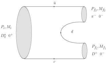
Figure 1: Feynman diagram for the decay channel $D_{0}^{*}(2400)^{0}\to D^{+}\pi^{-}$.

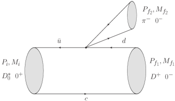
Figure 2: Feynman diagram for $D_{0}^{*}(2400)^{0}\to D^{+}\pi^{-}$ (with the low-energy approximation).

By using the reduction formula, the transition matrix element can be written as

$$\begin{split}T=&\langle D^{+}(P_{f1})\pi^{-}(P_{f2})\left|D_{0}^{*}(P_{i})\right.\rangle\\ =&\int{\rm{d}}^{4}x{\rm{e}}^{{\rm{i}}P_{f2}\cdot x}(M_{f2}^{2}-P_{f2}^{2})\langle D^{+}(P_{f1})\left|\phi_{\pi}(x)\right|D_{0}^{*}(P_{i})\rangle,\end{split}$$ (2)

where, $\phi_{\pi}$ is the light pseudo-scalar meson field. By using the PCAC relation, the field can be expressed as Chang et al. (2005)

$$\phi_{\pi}(x)=\frac{1}{M_{f2}^{2}f_{\pi}}\partial^{\mu}(\overline{u}\gamma_{\mu}\gamma_{5}d),$$ (3)

where $M_{f2}$ is the mass of $\pi$, and $f_{\pi}$ is its decay constant.

Inserting Eq. (3) into Eq. (2), the transition matrix can be written as

$$\begin{split}T=&\frac{M_{f2}^{2}-P_{f2}^{2}}{M_{f2}^{2}f_{\pi}}\int{\rm{d}}^{4}x{\rm{e}}^{iP_{f2}\cdot x}\langle D^{+}(P_{f1})\left|\partial^{\mu}(\overline{u}\gamma_{\mu}\gamma_{5}d)\right|D_{0}^{*}(P_{i})\rangle\\ =&\frac{-{\rm{i}}P_{f2}^{\mu}(M_{f2}^{2}-P_{f2}^{2})}{M_{f2}f_{\pi}}\int{\rm{d}}^{4}x{\rm{e}}^{iP_{f2}\cdot x}\langle D^{+}(P_{f1})\left|\overline{u}\gamma_{\mu}\gamma_{5}d\right|D_{0}^{*}(P_{i})\rangle.\end{split}$$ (4)

According to the low energy theorem Chang et al. (2005), the momentum of the light meson is much smaller than its mass and can be ignored. Then the Feynman diagram turns to Fig. 2 and the amplitude can be written as

$$\begin{split}T\approx&-{\rm{i}}\frac{P_{f2}^{\mu}}{f_{\pi}}\int{\rm{d}}^{4}x{\rm{e}}^{{\rm{i}}P_{f2}\cdot x}\langle D^{+}(P_{f1})\left|\overline{u}\gamma_{\mu}\gamma_{5}d\right|D_{0}^{*}(P_{i})\rangle\\ =&-{\rm{i}}\frac{P_{f2}^{\mu}}{f_{\pi}}(2\pi)^{4}\delta^{4}(P_{i}-P_{f1}-P_{f2})\langle D^{+}(P_{f1})\left|\overline{u}\gamma_{\mu}\gamma_{5}d\right|D_{0}^{*}(P_{i})\rangle.\end{split}$$ (5)

Besides using the PCAC rule and low energy theorem, we also use the effective Lagrangian method to get the transition amplitude of this process and the results of these two approaches are consistent. The Lagrangian is introduced by Zhong and Zhao (2010); Wang et al. (2017); Li et al. (2018),

$$\mathcal{L}_{qqP}=\frac{g}{\sqrt{2}f_{h}}\bar{q}_{i}\gamma^{\xi}\gamma^{5}q_{j}\partial_{\xi}\phi_{ij},$$ (6)

where

$$\phi_{ij}=\sqrt{2}\left[\begin{matrix}\frac{1}{\sqrt{2}}\pi^{0}+\frac{1}{\sqrt{6}}\eta&\pi^{+}&K^{+}\\ \pi^{-}&\-\frac{1}{\sqrt{2}}\pi^{0}+\frac{1}{\sqrt{6}}\eta&K^{0}\\ K^{-}&K^{0}&-\frac{2}{\sqrt{6}}\eta\end{matrix}\right]$$ (7)

is the chiral field of the pseudoscalar meson. The quark-meson coulping constant $g$ is taken to be unity and $f_{h}$ is the decay constant.

Within Mandelstam formalism Mandelstam (1955), we can write the hadronic transition amplitude as the overlap integral over the relativistic wave functions of the initial and final mesons Chang et al. (2006)

$$\begin{split}\mathcal{M}=&-{\rm{i}}\frac{P_{f2}^{\mu}}{f_{\pi}}\langle D^{+}(P_{f1})\left|\overline{u}\gamma_{\mu}\gamma_{5}d\right|D_{0}^{*}(P_{i})\rangle\\ =&-{\rm{i}}\frac{P_{f2}^{\mu}}{f_{\pi}}\int\frac{{\rm{d}}^{3}q}{(2\pi)^{3}}\mathrm{Tr}\left[\overline{\varphi}_{P_{f1}}^{++}({q}_{f1\perp})\frac{\not{P}_{i}}{M_{i}}\varphi_{P_{i}}^{++}({q}_{\perp})\gamma_{\mu}\gamma_{5}\right],\end{split}$$ (8)

where $q$ and ${q}_{f1}$ are the relative momenta between quark and anti-quark in initial and final meson, respectively. For the initial meson $D^{*}_{0}(c\bar{u})$, $q=p_{c}-\frac{m_{c}}{m_{u}+m_{c}}P_{i}=\frac{m_{u}}{m_{u}+m_{c}}P_{i}-p_{u}$, where $m_{u}$, $m_{c}$ are the quark masses and $p_{u}$ and $p_{c}$ are the quark momenta. And for the final meson $D^{+}(c\bar{d})$, due to the conservation law of momentum, its internal relative momentum is related to that of the initial meson by $q_{f1}=q-\frac{m_{c}}{m_{c}+m_{d}}P_{f1}$. Then, only the BS wave functions in the transition amplitude need to be figured out.

The BS equation of two-body bound state can read in momentum space as Salpeter and Bethe (1951); Li et al. (2017a)

$$S_{1}^{-1}\chi_{P}(q)S_{2}^{-1}={\rm{i}}\int\frac{{\rm{d}}^{4}k}{(2\pi)^{4}}I(P;q,k)\chi_{P}(k),$$ (9)

where $\chi_{P}(q)$ is the four-dimensional BS wave function; $I(P;q,k)$ is the interaction kernel; $S_{1}$ and $S_{2}$ are the propagators for the quark and anti-quark respectively.

We follow Salpeter Salpeter (1952) to take the instantaneous approximation $I(P;q,k)\approx I(q_{\perp}-k_{\perp})$ The three-dimensional salpeter wave function $\psi(q_{\perp})$ is defined by

$$\psi(q_{\perp})={\rm{i}}\int\frac{{\rm{d}}q_{P}}{2\pi}\chi_{P}(q),\quad\chi_{P}(q)=S_{1}(p_{1})\int\frac{{\rm{d}}^{3}k}{(2\pi)^{3}}I(q_{\perp}-k_{\perp})\psi_{P}(k_{\perp})S_{2}(p_{2})$$ (10)

In this work, we adopt the Cornell potential as the interaction kernel $I(r)$ as follow form Kim and Wang (2004); Li et al. (2017a)

$$I(r)=V_{s}(r)+V_{0}+\gamma_{0}\otimes\gamma^{0}V_{v}(r)=\frac{\lambda}{\alpha}(1-{\rm{e}}^{-\alpha r})+V_{0}-\frac{4}{3}\frac{\alpha_{s}}{r}{\rm{e}}^{-\alpha r},$$ (11)

where $\lambda$ is the string constant, $\alpha_{s}(r)$ is the running strong coupling constant and $V_{0}$ is an adjustable parameter fixed by the meson’s mass. In momentum space, the potential can read as

$$I(\vec{q})=-\left(\frac{\lambda}{\alpha}+V_{0}\right)(2\pi)^{3}\delta^{3}(\vec{q})+\frac{\lambda}{\pi^{2}}\frac{1}{(\vec{q}^{2}+\alpha^{2})^{2}}-\frac{2}{3\pi^{2}}\frac{\alpha_{s}(\vec{q})}{(\vec{q}^{2})+\alpha^{2}},$$ (12)

where the coupling constant $\alpha_{s}(\vec{q})$ is defined by:

$$\alpha_{s}(\vec{q})=\frac{12\pi}{27}\frac{1}{\log(\alpha+\frac{\vec{q}^{2}}{\Lambda_{QCD}^{2}})}.$$ (13)

In the above process, we take the instantaneous approximation in the interaction kernel, where we omit the retardation effect. According to the results of paper Qiao et al. (1996, 1999); Ebert et al. (2000), this effect affects much on the light mesons, but has limited influence on the heavy-flavor mesons, because these mesons have larger mass values. In addition, retardation effect mainly affects the mass spectra prediction. When we calculate the decay width, we adjust the $V_{0}$ to match the experimental data, which further reduces this effect. The results of our previous work Fu et al. (2011); Li et al. (2017a) are agree with experimental data very well, so the instantaneous approximation is applicable for heavy-light mesons.

Then, we express the relativistic wave function of a scalar meson with instantaneous approximation ($P_{i}\cdot q=0$) as

$$\varphi_{0^{+}}(q_{\perp})=M\left[\frac{\not{q}_{\perp}}{M}f_{a1}(q_{\perp})+\frac{\not{P}\not{q}_{\perp}}{M^{2}}f_{a2}(q_{\perp})+f_{a3}(q_{\perp})+\frac{\not{P}}{M}f_{a4}(q_{\perp})\right],$$ (14)

where $f_{ai}$($i=1,2,3,4$) are the functions of $q_{\perp}^{2}$ and their value can be obtained by solving the full Salpeter equations. It is notable that $\varphi_{0^{+}}(q_{\perp})$ is a general form for $J^{P}=0^{+}$ states and the items containing $q$ are the high order relativistic corrections.

Within BS method, the four wave functions $f_{ai}$ are not independent, they have the following relations Wang (2009)

$$\begin{split}&f_{a3}=\frac{q_{\perp}^{2}(\omega_{1}+\omega_{2})}{M(m_{1}\omega_{2}+m_{2}\omega_{1})}f_{a1},\\ &f_{a4}=\frac{q_{\perp}^{2}(\omega_{1}-\omega_{2})}{M(m_{1}\omega_{2}+m_{2}\omega_{1})}f_{a2},\end{split}$$ (15)

where $m_{1}=m_{c}$, $m_{2}=m_{u}$, $\omega_{1}=\sqrt{m_{1}^{2}-{q}_{\perp}^{2}}$, and $\omega_{2}=\sqrt{m_{2}^{2}-{q}_{\perp}^{2}}$.

In our calculation, we only keep the positive energy parts $\varphi_{P_{i}}^{++}({q}_{i\perp})$ of the relativistic wave functions because the negative energy part contributes too small Wang et al. (2017). The positive energy part of the wave function can be written as

$$\varphi_{0^{+}}^{++}(q_{\perp})=A_{1}+A_{2}\frac{\not{P}}{M}+A_{3}\frac{\not{q}_{\perp}}{M}+A_{4}\frac{\not{P}\not{q}_{\perp}}{M^{2}},$$ (16)

where

$$\begin{split}A_{1}=&\;\frac{(\omega_{1}+\omega_{2})q^{2}_{\perp}}{2(m_{1}\omega_{2}+m_{2}\omega_{1})}\left(f_{a1}+\frac{m_{1}+m_{2}}{\omega_{1}+\omega_{2}}f_{a2}\right),\\ A_{2}=&\ \frac{(m_{1}-m_{2})q^{2}_{\perp}}{2(m_{1}\omega_{2}+m_{2}\omega_{1})}\left(f_{a1}+\frac{m_{1}+m_{2}}{\omega_{1}+\omega_{2}}f_{a2}\right),\\ &A_{3}=\frac{M}{2}\left(f_{a1}+\frac{m_{1}+m_{2}}{\omega_{1}+\omega_{2}}f_{a2}\right),\\ &A_{4}=\frac{M}{2}\left(\frac{\omega_{1}+\omega_{2}}{m_{1}+m_{2}}f_{a1}+f_{a2}\right).\end{split}$$ (17)

To calculate the values of wave functions, we should determine the parameters’ values in the interaction kernel. We try to fix $V_{0}$ by the mass of the ground state. In this case, the theoretical mass of $D_{J}^{*}(3000)$ is much less than the present experimental data. Thus, we adjust $V_{0}$ to make its mass value be equal to the experimental data, then get the wave functions. In this work, besides the wave function for $0^{+}$ state, we also need the wave functions of $0^{-}$, $1^{-}$, $1^{+}$, etc., which are presented in the appendix.

After finishing the integral, we can get the amplitude of $0^{+}\to 0^{-}0^{-}$ as follow

$$\begin{split}\mathcal{M}_{(0^{+}\to 0^{-}0^{-})}=-{\rm{i}}\frac{P_{f2}^{\mu}}{f_{\pi}}(P_{\mu}n_{1}+P_{f1\mu}n_{2}),\end{split}$$ (18)

where $n_{1}$ and $n_{2}$ are the form factors. They are the overlap integral over the wave functions of the initial and final states.

If the final light meson is $\eta$ or $\eta^{\prime}$, the $\eta-\eta^{\prime}$ mixing should be considered

$$\left(\begin{array}[]{c}\eta\\ \eta^{\prime}\end{array}\right)=\left(\begin{array}[]{cc}\cos\theta_{P}&-\sin\theta_{P}\\ \sin\theta_{P}&\cos\theta_{P}\end{array}\right)\left(\begin{array}[]{c}\eta_{8}\\ \eta_{1}\end{array}\right),$$ (19)

where $\eta_{1}=(u\bar{u}+d\bar{d}+s\bar{s})/{\sqrt{3}}$ and $\eta_{8}={(u\bar{u}+d\bar{d}-2s\bar{s})}/{\sqrt{6}}$, we choose the mixing angle $\theta_{P}=-11.4^{\circ}$ C. Patrignani et al. (2016). Then, we get the transition amplitude with an extra coefficient after considering the mixing

$$\begin{split}\mathcal{M}(\eta)=-{\rm{i}}P_{f2}^{\mu}M^{2}_{\eta}\left(\frac{\cos\theta_{P}}{\sqrt{6}f_{\eta_{8}}M^{2}_{\eta_{8}}}-\frac{\sin\theta_{P}}{\sqrt{3}f_{\eta_{1}}M^{2}_{\eta_{1}}}\right)\langle D^{0}(P_{f1})\left|\overline{u}\gamma_{\mu}\gamma_{5}u\right|D_{0}^{*}(P_{i})\rangle,\\ \mathcal{M}(\eta^{\prime})=-{\rm{i}}P_{f2}^{\mu}M^{2}_{\eta^{\prime}}\left(\frac{\sin\theta_{P}}{\sqrt{6}f_{\eta_{8}}M^{2}_{\eta_{8}}}+\frac{\cos\theta_{P}}{\sqrt{3}f_{\eta_{1}}M^{2}_{\eta_{1}}}\right)\langle D^{0}(P_{f1})\left|\overline{u}\gamma_{\mu}\gamma_{5}u\right|D_{0}^{*}(P_{i})\rangle.\end{split}$$ (20)

In the case when heavy-light $1^{+}$ state is involved, if we use the $S$-$L$ coupling, the ${}^{3}P_{1}$ and ${}^{1}P_{1}$ states cannot describe the physical states. Within the heavy quark limit($m_{Q}\to\infty$), its spin decouples and the properties of the heavy-light $1^{+}$ state are determined by those of the light quarks. So $j$-$j$ coupling should be used instead. The orbital angular momentum $\vec{L}$ couples with the light quark spin $\vec{s}_{q}$, which is $\vec{j}_{l}=\vec{L}+\vec{s}_{q}$. Then $1^{+}$ state can be grouped into a doublet by the total angular momentum of the light quark($|j_{l}=1/2\rangle$ and $|j_{l}=3/2\rangle$). The relation between the two descriptions are Matsuki et al. (2010); Barnes et al. (2005)

$$\left(\begin{array}[]{c}|J^{P}=1^{+},j_{l}={3}/{2}\rangle\\ |J^{P}=1^{+},j_{l}={1}/{2}\rangle\\ \end{array}\right)=\left(\begin{array}[]{cc}\cos\theta&\sin\theta\\ -\sin\theta&\cos\theta\\ \end{array}\right)\left(\begin{array}[]{c}|{{}^{1}}P_{1}\rangle\\ |{{}^{3}}P_{1}\rangle\\ \end{array}\right).$$ (21)

In our method, we solve the Salpeter equations for ${}^{3}P_{1}$ and ${}^{1}P_{1}$ states individually, and use these mixing relations to calculate the contributions of two physical $1^{+}$ states. We list some mixing states related to our work

$$\left(\begin{array}[]{c}D_{1}(2420)\\ D_{1}(2430)\\ \end{array}\right)=\left(\begin{array}[]{cc}\cos\theta&\sin\theta\\ -\sin\theta&\cos\theta\\ \end{array}\right)\left(\begin{array}[]{c}D(1{{}^{1}}P_{1})\\ D(1{{}^{3}}P_{1})\\ \end{array}\right),$$ (22)

$$\left(\begin{array}[]{c}D_{s1}(2536)\\ D_{s1}(2460)\\ \end{array}\right)=\left(\begin{array}[]{cc}\cos\theta&\sin\theta\\ -\sin\theta&\cos\theta\\ \end{array}\right)\left(\begin{array}[]{c}D_{s}(1{{}^{1}}P_{1})\\ D_{s}(1{{}^{3}}P_{1})\\ \end{array}\right).$$ (23)

In our calculation, for these doublets, we choose the ideal mixing angle $\theta=35.3^{\circ}$ in the heavy quark limit.

For the ${}^{3}P_{1}(1^{++})$ and ${}^{1}P_{1}(1^{+-})$ states, the corresponding hadronic transition amplitudes are

$$\begin{split}\mathcal{M}_{(0^{+}\to 1^{++}0^{-})}=\frac{-{\rm{i}}}{f_{\pi}}\varepsilon_{1\mu}P^{\mu}t_{1},\\ \mathcal{M}_{(0^{+}\to 1^{+-}0^{-})}=\frac{-{\rm{i}}}{f_{\pi}}\varepsilon_{1\mu}P^{\mu}t_{2},\end{split}$$ (24)

where $\varepsilon$ is the polarization vector of the $1^{+}$ state; $t_{1}$ and $t_{2}$ are the form factors. Then, the form factors of the physical states are

$$\begin{split}t_{D_{1}(2420),D_{s1}(2536)}=t_{2}\cos\theta+t_{1}\sin\theta,\\ t_{D_{1}(2430),D_{s1}(2460)}=-t_{2}\sin\theta+t_{1}\cos\theta.\end{split}$$ (25)

The PCAC rule can only be applied to light pseudo-scalar mesons and it is not valid for light vector meson. If $\rho$ or $\omega$ meson appears in the final states, we choose the effective Lagrangian method to calculate the transition amplitude. The Lagrangian of quark-meson coupling can be expressed as Zhong and Zhao (2010); Wang et al. (2017); Li et al. (2018)

$$\mathcal{L}_{qqV}=\bar{q}_{i}(a\gamma_{\mu}+\frac{{\rm{i}}b}{2M_{P_{f2}}}\sigma_{\mu\nu}P_{f2}^{\nu})V_{ij}^{\mu}q_{j},$$ (26)

where $V^{\mu}_{ij}$ is the field of the light vector meson; $q_{i}$ and $\bar{q}_{j}$ are its constitute quarks. And we choose the parameters $a=-3$ and $b=2$ which represent the vector and tensor coupling strength Wang et al. (2017), respectively. Then we use Eq. (26) to derive the light-vector meson’s vertex and get the transition amplitude

$$\begin{split}\mathcal{M}=-{\rm{i}}\int\frac{{\rm{d}}^{3}q}{(2\pi)^{3}}\mathrm{Tr}\left[\overline{\varphi}_{P_{f1}}^{++}({q}_{f1\perp})\frac{\not{P}_{i}}{M_{i}}\varphi_{P_{i}}^{++}({q}_{\perp})(a\gamma_{\mu}+\frac{{\rm{i}}b}{2M_{f2}}\sigma_{\mu\nu}P_{f2}^{\nu})\varepsilon_{2}^{\mu}\right].\end{split}$$ (27)

After finishing the trace and integral, the transition amplitudes can be expressed as

$$\begin{split}\mathcal{M}_{(0^{+}\to 1^{-}1^{-})}=\varepsilon_{1\mu}\varepsilon_{2}^{\mu}t_{1}+\varepsilon_{1\mu}P^{\mu}\varepsilon_{2\nu}P^{\nu}t_{2},\end{split}$$ (28)

where $\varepsilon_{1\mu}$ and $\varepsilon_{2\nu}$ are the polarization vectors of final heavy vector meson and the light vector meson, respectively; $t_{1}$, $t_{2}$ and $t_{3}$ are the form factors.

Then, the two-body decay width can be expressed as

$$\begin{split}\Gamma=\frac{1}{8\pi}\frac{|\vec{P}_{f1}|}{M^{2}_{i}}|\mathcal{M}|^{2},\end{split}$$ (29)

where $\vec{P}_{f1}$ is the three-dimensional momentum of the final charmed meson

$$|\vec{P}_{f1}|=\sqrt{\left(\frac{M_{i}^{2}+M_{f1}^{2}-M_{f2}^{2}}{2M_{i}}\right)^{2}-M_{f1}^{2}}.$$ (30)

III Results and Discussions

In this paper, the masses of constituent quarks that we adopt are listed as follows: $m_{u}=0.305{\ \rm{GeV}},\ m_{d}=0.311{\ \rm{GeV}},\ m_{s}=0.50{\ \rm{GeV}},\ {\rm and}~{}m_{c}=1.62{\ \rm{GeV}}$ Wang et al. (2013). Other parameters are $\alpha=0.060{\ \rm{GeV}}$, $\lambda=0.210{\ \rm{GeV}}^{2}$, $\Lambda_{QCD}=0.270{\ \rm{GeV}}$, $f_{\pi}=0.1304{\ \rm{GeV}}$, $f_{K}=0.1562{\ \rm{GeV}}$ C. Patrignani et al. (2016), $f_{\eta_{1}}=1.07f_{\pi}$, $f_{\eta_{8}}=1.26f_{\pi}$, $M_{\eta_{1}}=0.923{\ \rm{GeV}}$, and $M_{\eta_{8}}=0.604{\ \rm{GeV}}$ Wang et al. (2017). The masses of other involved mesons are shown in Table 3.

Table 3: Masses of involved mesons ($\mathrm{GeV}$) C. Patrignani et al. (2016).

$m_{D_{0}^{*}(2400)^{0}}=2.318$	$m_{D_{0}^{*}(2400)^{+}}=2.351$	$m_{D_{J}^{*}(3000)^{(0,+)}}=3.008$	$m_{D_{s}^{+}}=1.968$
$m_{D_{1}(2420)^{0}}=2.421$	$m_{D_{1}(2420)^{+}}=2.423$	$m_{D_{1}(2430)^{(0,+)}}=2.427$	$m_{D_{s}^{*+}}=2.112$

We first calculate the the decay widths of the $1P$ states. It only have two OZI-allowed decay channels and the results are presented in Table 4. In the case of $D_{0}^{*}(2400)^{0}$, the decay width of $D^{+}\pi^{-}$ is almost twice as that of $D^{0}\pi^{0}$. Because there is a factor $1/\sqrt{2}$ in the constitute quarks of $\pi^{0}$. Other decays that involve $\rho^{0}$ and $\omega^{0}$ have similar relation too.

Table 4: $D_{0}^{*}(2400)^{0,+}$ strong decay widths (MeV). Ref. Zhong and Zhao (2008) adopts Chiral Quark Model, Ref. Close and Swanson (2005) adopts the ${}^{3}P_{0}$ Model and Ref. Godfrey (2005) adopts the Pseudoscalar Emission Model.

Chanel		Ours	Ref. Zhong and Zhao (2008)	Ref. Close and Swanson (2005)	Ref. Godfrey (2005)	Exp. C. Patrignani et al. (2016)
$D_{0}^{*}(2400)^{0}\to$	$D^{+}\pi^{-}$	151.5	266	283	277	$267\pm 40$
	$D^{0}\pi^{0}$	74.8
$D_{0}^{*}(2400)^{+}\to$	$D^{+}\pi^{0}$	81.6	$\Box$	$\Box$	$\Box$	$230\pm 17$
	$D^{0}\pi^{+}$	164.3

The total decay width of $D_{0}^{*}(2400)^{+}$ is larger than that of $D_{0}^{*}(2400)^{0}$ in our calculation, which are 245.9 MeV and 226.3 MeV, respectively. According to the present experimental data, the charged $D_{0}^{*}(2400)^{+}$ is heavier than the neutral $D_{0}^{*}(2400)^{0}$. The different phase spaces may result in this discrepancy. We also notice that the estimated decay widths are sensitive to the mass of the initial meson. Considering the experimental mass values have errors ($m_{D_{0}^{*}(2400)^{0}}=2318\pm 29\ \mathrm{MeV},\ m_{D_{0}^{*}(2400)^{\pm}}=2351\pm\ 7\mathrm{MeV}$ C. Patrignani et al. (2016)) and these experimental masses value have divergence with different theoretical predictionsGodfrey and Isgur (1985); Di Pierro and Eichten (2001); Ebert et al. (2009); Sun et al. (2013); Godfrey and Moats (2016), we give the two-body decay width changing along with the initial meson mass from 2300 MeV to 2420 MeV, which is shown in Fig. 3(a). The neutral one’s total decay width changes from 214.0 to 287.2 MeV, and the charged one’s is from 212.7 to 289.0 MeV . We believe that these OZI-allowed decays happen around the mass threshold, which results in such sensitivity of decay width to the initial $1P$ state mass.

In Table 4, we also list the results from other models Godfrey (2005); Zhong and Zhao (2008); Close and Swanson (2005) as well as the experimental results for comparison. According to Table 4 and Fig. 3(a), we conclude that our results of the $1P$ states are consistent with experimental data, which means we can apply the same method to study the $2P$ states.

Table 5: Two-body strong decay widths (MeV) of $D_{J}^{*}(3000)^{0}$ as the $2P(0^{+})$ state. “-” means the channel is forbidden, “$\Box$” means the channel is not included by this method. Ref. Yu et al. (2015) uses ${}^{3}P_{0}$ Model; Ref. Sun et al. (2013) uses QPC Model; Ref. Godfrey and Moats (2016) uses Relativistic quark model and Ref. Gupta and Upadhyay (2018). uses effective Lagrangian approach.

Chanel	Final States	Ours	Ref. Yu et al. (2015)	Ref. Sun et al. (2013)	Ref. Godfrey and Moats (2016)	Ref. Gupta and Upadhyay (2018)
$D(^{1}S_{0})\pi$	$D^{+}\pi^{-}$	11.6	23.94	49	25.4	66.2
	$D^{0}\pi^{0}$	6.1	11.97			33.3
$D(2^{1}S_{0})\pi$	$D(2550)^{+}\pi^{-}$	6.9	$\Box$	$\Box$	18.6	$\Box$
	$D(2550)^{0}\pi^{0}$	3.3
$D\eta$	$D^{0}\eta^{0}$	0.51	4.26	8.8	1.53	10.8
$D\eta^{\prime}$	$D^{0}\eta^{\prime 0}$	6.0	1.07	2.7	4.94	$\Box$
$D_{s}K$	$D_{s}^{+}K^{-}$	~$10^{-3}$	2.85	6.6	0.76	54.2
$D_{1}(2420)\pi$	$D_{1}(2420)^{0}\pi^{0}$	18.7	26.20	38	96.1$(^{1}P_{1})$	$\Box$
	$D_{1}(2420)^{+}\pi^{-}$	36.8	$\Box$
$D_{1}(2420)\eta$	$D_{1}(2420)^{0}\eta^{0}$	0.85	1.37	1.1	$\Box$	$\Box$
$D_{1}(2430)\pi$	$D_{1}(2430)^{0}\pi^{0}$	2.1	6.69	30	$\Box$	$\Box$
	$D_{1}(2430)^{+}\pi^{-}$	4.1	$\Box$
$D_{1}(2430)\eta$	$D_{1}(2430)^{0}\eta^{0}$	0.12	0.35	0.91	$\Box$	$\Box$
$D_{s}(2460)K$	$D_{s1}(2460)^{+}K^{-}$	1.2	12.81	1.5	$\Box$	$\Box$
$D^{*}\rho$	$D^{*}(2007)^{0}\rho^{0}$	7.0	31.60	41	32	$\Box$
	$D^{*}(2010)^{+}\rho^{-}$	13.3	62.01
$D^{*}\omega$	$D^{*}(2007)^{0}\omega^{0}$	7.5	29.91	13	10.2	$\Box$
$D_{s}^{*}K^{*}$	$D_{s}^{*+}K^{*}(892)^{-}$	4.1	3.06	1.0	$\Box$	$\Box$
$D_{s}(2536)K^{-}$	$D_{s1}(2536)^{+}K^{-}$	-	6.40	-	-	-
Total		130.2	224.5	193.6	189.5	164.5
Experimental value		$110.5\pm 11.5$

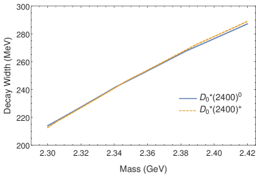
(a) $\Gamma_{D_{0}^{*}(2400)^{(0,+)}}$ versus the mass

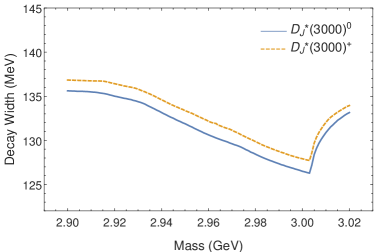
(b) $\Gamma_{D_{J}^{*}(3000)^{(0,+)}}$ versus the mass

Figure 3: Total decay widths of $D_{0}^{*}(2400)$ and $D_{J}^{*}(3000)$ change with the masses.

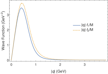
(a) $0^{+}$($1P$) state $D_{0}^{*}(2400)^{0}$

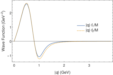
(b) $0^{+}$($2P$) state $D_{J}^{*}(3000)^{0}$

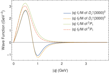
(c) $D_{J}^{*}(3000)^{0}$ and $D_{1}(2420)$(${}^{3}P_{1}$ state)

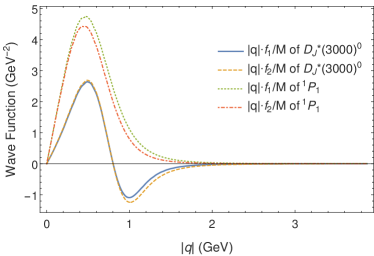
(d) $D_{J}^{*}(3000)^{0}$ and $D_{1}(2420)$(${}^{1}P_{1}$ state)

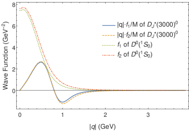
(e) $D_{J}^{*}(3000)^{0}$ and $D^{0}$(${}^{1}S_{0}$ state)

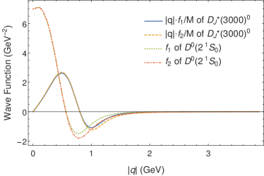
(f) $D_{J}^{*}(3000)^{0}$ and $D^{0}$($2^{1}S_{0}$ state)

Figure 4: Several examples of wave functions for some states

Under the assumption of $0^{+}$($2P$) state, the results of ours and other models are shown in Table 5. The total width of our calculation is 130.2 MeV, which is smaller than the results of other models and close to the upper limit of experimental value. Though the $2P$ state $D_{J}^{*}(3000)^{0}$ has larger phase space and more decay channels than those of $1P$ state $D_{0}^{*}(2400)^{0}$, why we get a narrower full width? The reason is the different structures of wave functions. The numerical values of the wave functions $f_{a1}$ and $f_{a2}$ for $1P$ state as the function of internal momentum $|\vec{q}|$ are all positive (Fig. 4(a)), while the wave functions of the $2P$ state have a node (Fig. 4(b)). The wave function values after the node become negative and it makes contrary contribution to the positive part, which will cause cancellation in the overlap integral between these two parts. The node structure reduces the decay width of the $2P$ state.

From our results, the channels of $D\pi,\ D_{1}(2420)\pi,\ D\rho$ give large contribution to the full decay width, and $D_{1}(2420)\pi$ channel is dominant. As shown in Eq. (8), large transition amplitude means that these three channels have large overlap integrals. For example, we draw the wave functions of final state $D_{1}(2420)(^{3}P_{1}\&^{1}P_{1})$ and initial $D_{J}^{*}(3000)$ in Fig. 4(c) and 4(d). When the recoil momentum of the final meson is small (ignoring the difference between internal momenta of the initial and final states here), the peak values of the initial and final wave functions are coincident. Thus, we obtain large overlap integral values of the wave functions before the $2P$ node. However, the part after the node gives small cancellation since the corresponding values of the $1P$ wave function are small at this time. As a result, we obtain a large decay width of $D_{1}(2420)\pi$ channel.

Other examples of $D(1^{1}S_{0})$ and $D(2^{1}S_{0})$ are shown in Fig. 4(e) and 4(f). For the channel of $D(1^{1}S_{0})\pi$, when compared with $D_{1}(2420)\pi$, the part after the node gives negative contribution. Because the peak values of the those wave functions are not coincident, the positive contribution of the part before the node is not dominant. The negative part after the node changes the sign of the overlap integral, which cause the width of $D(1^{1}S_{0})\pi$ is narrower than that of $D_{1}(2420)\pi$. For the $D(2^{1}S_{0})\pi$ channel, both wave functions have node structure. Compared with $D(1^{1}S_{0})\pi$ channel, the contribution from the part before the $2P$ node is obviously smaller for $D(2^{1}S_{0})\pi$. But the contribution after the $2P$ node becomes positive again because both wave functions ($2S$ and $2P$ states) are negative at this time. Therefore, although the phase space is narrow, the decay width of $D(2^{1}S_{0})\pi$ channel is not very small.

It has been mentioned in Sec. I that the relativistic corrections are large for the excited states. We can explain this argument according to the figures of the wave functions. If contribution from large internal momentum $q$ is significant, we can conclude that relativistic corrections are considerable. In Fig. 4(e), for the $1S$ state, the peak value of the wave function appear in the region of small $q$, while for the $1P$ state, in Fig. 4(c) and 4(d), the peak values appear in the region of middle $q$. This means the $1P$ state has larger relativistic correction than that of the $1S$ ground state. When comparing Fig. 4(e) with 4(f), wave functions after the node give sizable contribution, which happens in large $q$ region. This means higher excited states have larger relativistic corrections. So we conclude that a relativistic model is needed to deal with the excited state problem.

In our study, we also calculate the decay widths of $D_{J}^{*}(3000)^{+}$, shown in Table 6. All channels are similar to $D_{J}^{*}(3000)^{0}$, and the full width is 131.3 MeV.

Table 6: Two-body strong decay widths (MeV) of $D_{J}^{*}(3000)^{+}$ as the $2P(0^{+})$ state.

Chanel	Final States	Width		Chanel	Final States	Width
$D(^{1}S_{0})\pi$	$D^{+}\pi^{0}$	6.5		$D(2^{1}S_{0})\pi$	$D^{0}\pi^{+}$	3.8
	$D^{0}\pi^{+}$	13.5			$D^{0}\pi^{+}$	7.7
$D\eta$	$D^{0}\eta^{0}$	0.56		$D\eta^{\prime}$	$D^{0}\eta^{\prime 0}$	5.7
$D(2420)\pi$	$D_{1}(2420)^{+}\pi^{0}$	18.3		$D(2430)\pi$	$D_{1}(2430)^{+}\pi^{0}$	2.1
	$D_{1}(2420)^{0}\pi^{+}$	37.4			$D_{1}(2430)^{0}\pi^{+}$	4.3
$D(2420)\eta$	$D_{1}(2420)^{+}\eta^{0}$	0.77		$D(2430)\eta$	$D_{1}(2430)^{+}\eta^{0}$	0.11
$D^{*}\rho$	$D^{*}(2010)^{+}\rho^{0}$	6.1		$D^{*}\omega$	$D^{*}(2010)^{+}\omega^{0}$	6.5
	$D^{*}(2007)^{0}\rho^{-}$	12.9		$D_{s}(2460)K$	$D_{s1}(2460)^{+}K^{0}$	1.2
$D_{s}K$	$D_{s}^{+}K^{0}$	0.05		$D_{s}^{*}K^{*}$	$D_{s}^{*+}K^{*}(892)^{0}$	3.8
Total			131.3

Considering many theoretical prediction of the mass are lower than 3000 MeV Godfrey and Isgur (1985); Di Pierro and Eichten (2001); Ebert et al. (2009); Sun et al. (2013); Godfrey and Moats (2016) and the properties of these states could be revised after more experimental data collected, we also calculate the total width changing with the mass from 2900 to 3020 MeV, which is shown in Fig. 3(b). The total width of the neutral one ranges from 135.6 to 126.3 MeV, while the charged one’s result changes from 136.8 to 127.7 MeV. The full width of the $2P$ state becomes narrower along with the phase space increasing, which is opposite to that of the $1P$ case. The reason is that the recoil momentum becomes more considerable when phase space is larger for the $2P$ state. This results in greater contribution from the part after the nodes, so the decay width gets smaller. We also notice that there is a rise at the tail of the curve. It is because some new channels open when the mass of $D_{J}^{*}(3000)$ increase to 3000 MeV, such as $D_{s}^{*}K^{*}$, $D_{1}(2420)\eta$, $D_{1}(2430)\eta$. Thus, the total widths have the sudden rise.

IV SUMMARY

In this work, we study the two-body strong decay properties of two orbitally excited scalar $D$ mesons by the improved BS method. Our results of the $D_{0}^{*}(2400)$, as the $0^{+}(1P)$ states, are consistent with the present experimental data, which shows the suitability of our method. However, the sensitivity of decay width to its mass means more precise measurements are needed. For the $0^{+}(2P)$ assignment of $D_{J}^{*}(3000)$, the full decay width is about 131 MeV, which is a little higher but close to the present experimental data. Besides the $D\pi$ mode, we find $D\rho$ and $D_{1}(2420)\pi$ channels also contribute much to the full width, and they can be helpful in the further investigation. Considering the theoretical uncertainties from relativistic corrections of highly excited states and the preliminary experimental data at present, $D_{J}^{*}(3000)$ is still a strong candidate for the $2^{3}P_{0}$ state. We expect more experimental and theoretical efforts on this newly discovered resonance.

APPENDIX Bethe-Salpeter Wave Function

BS method has been used extensively to describe the properties of heavy-light mesons Wang (2006, 2009). Here we only list some wave functions related to this work Kim and Wang (2004); Li et al. (2017b)

.1 Wave function of $0^{-}$ state

The general form of the wave function is

$$\varphi_{0^{-}}(q_{\perp})=M\left[\frac{\not{P}}{M}f_{b1}(q_{\perp})+f_{b2}(q_{\perp})+\frac{\not{q}_{\perp}}{M}f_{b3}(q_{\perp})+\frac{\not{P}\not{q}_{\perp}}{M^{2}}f_{b4}(q_{\perp})\right]\gamma_{5},$$ (A-1)

where constraint conditions are

$$\begin{split}&f_{b3}=\frac{M(\omega_{2}-\omega_{1})}{m_{1}\omega_{2}+m_{2}\omega_{1}}f_{b2},\\ &f_{b4}=-\frac{M(\omega_{1}+\omega_{2}}{m_{1}\omega_{2}+m_{2}\omega_{1}}f_{b1}.\end{split}$$ (A-2)

The positive part is expressed as

$$\varphi_{0^{-}}^{++}(q_{\perp})=\left[B_{1}(q_{\perp})+\frac{\not{P}}{M}B_{2}(q_{\perp})+\frac{\not{P}}{M}B_{3}(q_{\perp})+\frac{\not{P}\not{q}_{\perp}}{M^{2}}B_{4}(q_{\perp})\right]\gamma_{5}.$$ (A-3)

where

$$\begin{split}&B_{1}\;=\frac{M}{2}\left(\frac{\omega_{1}+\omega_{2}}{m_{1}+m_{2}}f_{b1}+f_{b2}\right),\\ &B_{2}\;=\frac{M}{2}\left(f_{b1}+\frac{m_{1}+m_{2}}{\omega_{1}+\omega_{2}}f_{b2}\right),\\ &B_{3}=-\frac{M(\omega_{1}-\omega_{2})}{m_{1}\omega_{2}+m_{2}\omega_{1}}B_{1},\\ &B_{4}=-\frac{(m_{1}+m_{2})M}{m_{1}\omega_{2}+m_{2}\omega_{1}}B_{1}.\end{split}$$ (A-4)

.2 Wave function of $1^{+}$ state

We separate pseudo-vector $1^{+}$ state into $1^{++}$ and $1^{+-}$ to discuss. The general form of $1^{++}(^{3}P_{1})$ state is

$$\varphi_{1^{++}}(q_{\perp})={\rm{i}}\varepsilon_{\mu\nu\alpha\beta}\frac{P^{\nu}}{M}q^{\alpha}_{\perp}\epsilon^{\beta}\gamma^{\mu}\left[\gamma^{\mu}f_{c1}+\frac{\not{P}}{M}\gamma_{\mu}f_{c2}+\frac{q_{\perp}}{M}\gamma^{\mu}f_{c3}+\frac{\not{P}\gamma^{\mu}\not{q}_{\perp}}{M^{2}}f_{c4}\right],$$ (B-5)

where constraint conditions are

$$\begin{split}&f_{c3}=-\frac{M(\omega_{1}-\omega_{2})}{m_{1}\omega_{2}+m_{2}\omega_{1}}f_{c1},\\ &f_{c4}=\frac{M(\omega_{1}+\omega_{2})}{m_{1}\omega_{2}+m_{2}\omega_{1}}f_{c2}.\end{split}$$ (B-6)

The positve part of the wave function is

$$\varphi^{++}_{1^{++}}(q_{\perp})={\rm{i}}\varepsilon_{\mu\nu\alpha\beta}\frac{P^{\nu}}{M}q^{\alpha}_{\perp}\epsilon^{\beta}\gamma^{\mu}\left[C_{1}(q_{\perp})+\frac{\not{P}}{M}C_{2}(q_{\perp})+\frac{q_{\perp}}{M}C_{3}(q_{\perp})+\frac{\not{P}\not{q}_{\perp}}{M^{2}}C_{4}(q_{\perp})\right].$$ (B-7)

where the conefficients are

$$\begin{split}&C_{1}\,=\frac{1}{2}\left(f_{c1}+\frac{\omega_{1}+\omega_{2}}{m_{1}+m_{2}}f_{c2}\right),\\ &C_{2}\,=-\frac{1}{2}\left(\frac{m_{1}+m_{2}}{\omega_{1}+\omega_{2}}f_{c1}+f_{c2}\right),\\ &C_{3}=\frac{M(\omega_{1}-\omega_{2})}{m_{1}\omega_{2}+m_{2}\omega_{1}}C_{1},\\ &C_{4}=-\frac{M(m_{1}+m_{2})}{m_{1}\omega_{2}+m_{2}\omega_{1}}C_{1}.\end{split}$$ (B-8)

And the general form of $1^{+-}(^{1}P_{1})$ state is

$$\varphi_{1^{+-}}(q_{\perp})=q_{\perp}\cdot\epsilon\left[f_{d1}(q_{\perp})+\frac{\not{P}}{M}f_{d2}(q_{\perp})+\frac{\not{q}_{\perp}}{M}f_{d3}(q_{\perp})+\frac{\not{P}\not{q}_{\perp}}{M^{2}}f_{d4}(q_{\perp})\right]\gamma_{5},$$ (B-9)

Similar constraint condition is

$$\begin{split}f_{d3}=-\frac{M(\omega_{1}-\omega_{2})}{m_{1}\omega_{2}+m_{2}\omega_{1}}f_{d1},\\ f_{d4}=-\frac{M(\omega_{1}+\omega_{2})}{m_{1}\omega_{2}+m_{2}\omega_{1}}f_{d2}.\end{split}$$ (B-10)

The postive part of the wave function is

$$\varphi_{1^{+-}}^{++}(q_{\perp})=q_{\perp}\cdot\epsilon\left[D_{1}(q_{\perp})+\frac{\not{P}}{M}D_{2}(q_{\perp})+\frac{\not{q}_{\perp}}{M}D_{3}(q_{\perp})+\frac{\not{P}\not{q}_{\perp}}{M^{2}}D_{4}(q_{\perp})\right]\gamma_{5}.$$ (B-11)

where

$$\begin{split}&D_{1}=\frac{1}{2}\left(f_{d1}+\frac{\omega_{1}+\omega_{2}}{m_{1}+m_{2}}f_{d2}\right),\\ &D_{2}=\frac{1}{2}\left(\frac{m_{1}+m_{2}}{\omega_{1}+\omega_{2}}f_{d1}+f_{d2}\right),\\ &D_{3}=-\frac{M(\omega_{1}-\omega_{2})}{m_{1}\omega_{2}+m_{2}\omega_{1}}D_{1},\\ &D_{4}=-\frac{M(m_{1}+m_{2})}{m_{1}\omega_{2}+m_{2}\omega_{1}}D_{1}.\end{split}$$ (B-12)

.3 Wave function of $1^{-}$ state

The wave function of $1^{-}(^{3}S_{1})$ state is

$$\begin{split}\varphi_{1^{-}}(q_{\perp})=(q_{\perp}\cdot\varepsilon)\left[f_{e1}(q_{\perp})+\frac{\not{P}}{M}f_{e2}(q_{\perp})+\frac{\not{q}_{\perp}}{M}f_{e3}(q_{\perp})+\frac{\not{P}\not{q}_{\perp}}{M^{2}}f_{e4}(q_{\perp})\right]\\ +M\not{\varepsilon}\left[f_{e5}(q_{\perp})+\frac{\not{P}}{M}f_{e6}(q_{\perp})+\frac{\not{q}_{\perp}}{M}f_{e7}(q_{\perp})+\frac{\not{P}\not{q}_{\perp}}{M^{2}}f_{e8}(q_{\perp})\right].\end{split}$$ (C-13)

Constraint conditions are

$$\begin{split}f_{e1}=&\ \frac{q^{2}_{\perp}f_{e3}(\omega_{1}+\omega_{2})+2M^{2}f_{e5}\omega_{2}}{M(m_{1}\omega_{2}+m_{2}\omega_{1})},\\ f_{e2}=&\ \frac{q^{2}_{\perp}f_{e4}(\omega_{1}-\omega_{2})+2M^{2}f_{e6}\omega_{2}}{M(m_{1}\omega_{2}+m_{2}\omega_{1})},\\ &f_{e7}=\frac{M(\omega_{1}-\omega_{2}}{m_{1}\omega_{2}+m_{2}\omega_{1}}f_{e5},\\ &f_{e8}=\frac{M(\omega_{1}+\omega_{2})}{m_{1}\omega_{2}+m_{2}\omega_{1}}f_{e6}.\end{split}$$ (C-14)

The positive part of the wave function is

$$\begin{split}\varphi_{1^{-}}^{++}(q_{\perp})=(q_{\perp}\cdot\varepsilon)\left[E_{1}(q_{\perp})+\frac{\not{P}}{M}E_{2}(q_{\perp})+\frac{\not{q}_{\perp}}{M}E_{3}(q_{\perp})+\frac{\not{P}\not{q}_{\perp}}{M^{2}}E_{4}(q_{\perp})\right]\\ +M\not{\varepsilon}\left[E_{5}(q_{\perp})+\frac{\not{P}}{M}E_{6}(q_{\perp})+\frac{\not{q}_{\perp}}{M}E_{7}(q_{\perp})+\frac{\not{P}\not{q}_{\perp}}{M^{2}}E_{8}(q_{\perp})\right],\end{split}$$ (C-15)

where the coefficients are

$$\begin{split}&E_{1}=\frac{1}{2M(m_{1}\omega_{2}+m_{2}\omega_{1})}\left[(\omega_{1}+\omega_{2})q^{2}_{\perp}f_{e3}+(m_{1}+m_{2})q^{2}_{\perp}f_{e4}+2M^{2}\omega_{2}f_{e5}-2M^{2}m_{2}f_{e6}\right],\\ &E_{2}=\frac{1}{2M(m_{1}\omega_{2}+m_{2}\omega_{1}}\left[(m_{1}-m_{2})q^{2}_{\perp}f_{e3}+(\omega_{1}-\omega_{2})q^{2}_{\perp}f_{e4}-2M^{2}m_{2}f_{e5}+2M^{2}\omega_{2}f_{e6}\right],\\ &E_{3}=\frac{1}{2}\left[f_{e3}+\frac{m_{1}+m_{2}}{\omega_{1}+\omega_{2}}f_{e4}-\frac{2M^{2}}{m_{1}\omega_{2}+m_{2}\omega_{1}}f_{e6}\right],\\ &E_{4}=\frac{1}{2}\left[\frac{\omega_{1}+\omega_{2}}{m_{1}+m_{2}}f_{e3}+f_{e4}-\frac{2M^{2}}{m_{1}\omega_{2}+m_{2}\omega_{1}}f_{e5}\right],\\ &E_{5}=\frac{1}{2}\left[f_{e5}-\frac{\omega_{1}+\omega_{2}}{m_{1}+m_{2}}f_{e6}\right],\quad\quad E_{6}=\frac{1}{2}\left[-\frac{m_{1}+m_{2}}{\omega_{1}+\omega_{2}}f_{e5}+f_{e6}\right],\\ &E_{7}=\frac{M}{2}\frac{\omega_{1}-\omega_{2}}{m_{1}\omega_{2}+m_{2}\omega_{1}}\left[f_{e5}-\frac{\omega_{1}+\omega_{2}}{m_{1}+m_{2}}f_{e6}\right],\\ &E_{8}=\frac{M}{2}\frac{m_{1}+m_{2}}{m_{1}\omega_{2}+m_{2}\omega_{1}}\left[-f_{e5}+\frac{\omega_{1}+\omega_{2}}{m_{1}+m_{2}}f_{e6}\right].\end{split}$$ (C-16)

References

- J.M. Link et al. (2004) J.M. Link et al. (FOCUS Collaboration), Phys. Lett. B 586, 11 (2004).
- K. Abe et al. (2004) K. Abe et al. (Belle Collaboration), Phys. Rev. D 69, 112002 (2004).
- Close and Swanson (2005) F. E. Close and E. S. Swanson, Phys. Rev. D 72, 094004 (2005).
- Godfrey (2005) S. Godfrey, Phys. Rev. D 72, 054029 (2005).
- Zhong and Zhao (2008) X.-H. Zhong and Q. Zhao, Phys. Rev. D 78, 014029 (2008).
- R. Aaij et al. (2013) R. Aaij et al. (LHCb Collaboration), JHEP 2013, 145 (2013).
- Sun et al. (2013) Y. Sun, X. Liu, and T. Matsuki, Phys. Rev. D 88, 1 (2013).
- Lü and Li (2014) Q.-F. Lü and D.-M. Li, Phys. Rev. D 90, 054024 (2014).
- Yu et al. (2015) G.-L. Yu, Z.-G. Wang, Z.-Y. Li, and G.-Q. Meng, Chin. Phys. C 39, 063101 (2015).
- Godfrey and Moats (2016) S. Godfrey and K. Moats, Phys. Rev.D 93, 1 (2016).
- Li et al. (2018) S.-C. Li, T. Wang, Y. Jiang, X.-Z. Tan, Q. Li, G.-L. Wang, and C.-H. Chang, Phys. Rev. D 97, 054002 (2018).
- Chen et al. (2017) H.-X. Chen, W. Chen, X. Liu, Y.-R. Liu, and S.-L. Zhu, Rept. Prog. Phys. 80, 076201 (2017).
- Godfrey and Isgur (1985) S. Godfrey and N. Isgur, Phys. Rev. D 32, 189 (1985).
- Di Pierro and Eichten (2001) M. Di Pierro and E. Eichten, Phys. Rev. D 64, 114004 (2001).
- Ebert et al. (2009) D. Ebert, R. N. Faustov, and V. O. Galkin, Eur. Phys. J. C 66, 197 (2009).
- Song et al. (2015) Q.-T. Song, D.-Y. Chen, X. Liu, and T. Matsuki, Phys. Rev. D 92, 074011 (2015).
- Gupta and Upadhyay (2018) P. Gupta and A. Upadhyay, Phys. Rev. D97, 014015 (2018).
- Salpeter and Bethe (1951) E. E. Salpeter and H. A. Bethe, Phys. Rev. 84, 1232 (1951).
- Salpeter (1952) E. E. Salpeter, Phys. Rev. 87, 328 (1952).
- Kim and Wang (2004) C. S. Kim and G.-L. Wang, Phys. Lett. B584, 285 (2004).
- Wang et al. (2013) T. Wang, G.-L. Wang, H.-F. Fu, and W.-L. Ju, JHEP 2013, 120 (2013).
- Li et al. (2017a) Q. Li, Y. Jiang, T. Wang, H. Yuan, G.-L. Wang, and C.-H. Chang, Eur. Phys. J. C 77, 297 (2017a).
- Wang et al. (2017) T. Wang, Z.-H. Wang, Y. Jiang, L. Jiang, and G.-L. Wang, Eur. Phys. J. C 77, 38 (2017).
- Chang et al. (2005) C.-H. Chang, C. S. Kim, and G.-L. Wang, Phys. Lett. B 623, 218 (2005).
- Zhong and Zhao (2010) X.-H. Zhong and Q. Zhao, Phys. Rev. D 81, 014031 (2010).
- Mandelstam (1955) S. Mandelstam, Proc. R. Soc. Lond. A233, 248 (1955).
- Chang et al. (2006) C.-H. Chang, J.-K. Chen, and G.-L. Wang, Commun. Theor. Phys. 46, 467 (2006).
- Qiao et al. (1996) C.-f. Qiao, H.-W. Huang, and K.-T. Chao, Physical Review D 54, 2273 (1996).
- Qiao et al. (1999) C.-F. Qiao, H.-W. Huang, and K.-T. Chao, Physical Review D 60, 094004 (1999).
- Ebert et al. (2000) D. Ebert, R. N. Faustov, and V. O. Galkin, Phys. Rev. D 62, 034014 (2000).
- Fu et al. (2011) H.-F. Fu, G.-L. Wang, Z.-H. Wang, and X.-J. Chen, Chinese Physics Letters 28, 121301 (2011).
- Wang (2009) G.-L. Wang, Phys. Lett. B 674, 172 (2009).
- C. Patrignani et al. (2016) C. Patrignani et al. (Particle Data Group), Chin. Phys. C 40, 100001 (2016).
- Matsuki et al. (2010) T. Matsuki, T. Morii, and K. Seo, Prog. Theor. Phys. 124, 285 (2010).
- Barnes et al. (2005) T. Barnes, S. Godfrey, and E. S. Swanson, Phys. Rev. D 72, 1 (2005).
- Wang (2006) G.-L. Wang, Phys. Lett. B 633, 492 (2006).
- Li et al. (2017b) S.-C. Li, Y. Jiang, T.-H. Wang, Q. Li, Z.-H. Wang, and G.-L. Wang, Mod. Phys. Lett. A 32, 1750013 (2017b).