A Measurement Theory of Locality (MTL)

Abstract

Locality is a fundamental principle used extensively in program and system optimization. It can be measured in many ways. This paper formalizes the metrics of locality into a measurement theory. The new theory includes the precise definition of locality metrics based on access frequency, reuse time, reuse distance, working set, footprint, and the cache miss ratio. It gives the formal relation between these definitions and the proofs of equivalence or non-equivalence. It provides the theoretical justification for four successful locality models in operating systems, programming languages, and computer architectures which were developed empirically.

The manuscript is new and not a revision of a previous conference paper.

1 Introduction

Locality is a fundamental property of computation and a central principle in software, hardware and algorithmic design [Denning, 2005]. As defined by Denning, it is the “tendency for programs to cluster references to subsets of address space for extended periods.” [Denning and Martell, 2015, pp. 143]

Existing literature provides many ways to measure locality: reuse frequency, miss frequency, reuse distance, footprint and working set. They are intuitively related, i.e. data reuse in a program is likely to become data reuse in cache and therefore reduces the miss frequency. The relation, however, is not all clear. Some metrics, e.g. reuse distance, do not depend on cache size, but other metrics, e.g. miss ratio, do. Without a precise relation, we do not know which data reuse becomes a cache hit. As a result we do not have reliable properties. For example, it is possible to have more reuses in a program but fewer reuses in cache. Locality optimization cannot be sufficiently formulated without knowing how optimizing for one metric would affect other metrics.

In this paper, we give a measurement theory of locality (MTL) to formalize the relation between a set of locality metrics. Measurement of locality is the assignment of a number so that locality of different programs can be compared. The measurement theory consists of a set of locality metrics, the relation between them, and their precision and error.

The theory has a limited scope. It is a theory about locality measurements but not directly about locality optimization. It can compute the amount of data transfer in a memory hierarchy but does not minimize the amount of data transfer, nor does it optimize the data layout, which is a more complex problem (for either processor cache Petrank and Rawitz [2002] or virtual memory Lavaee [2016]). It assumes automatic cache management by least-recently used (LRU) replacement or similar policies. It does not solve the more general problem of I/O complexity Hong and Kung [1981]; Elango et al. [2015].

2 Measurement Theory of Locality

We will first present an overview that divides the locality measurements into six categories and then present them in subsections.

2.1 Overview

Figure 1 shows locality metrics in three top-level and four second-level categories. At the top level, access metrics are measures of locality for each memory access. The other two types are mathematical functions: timescale metrics, whose parameter is a length of time, and cache metrics, whose parameter is a cache size. For these metrics, the measurement theory gives their precise definitions and properties.

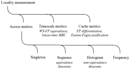
Figure 1: The categories of locality measurements and new theoretical results (in italics)

First, the paper formalizes access metrics into four second-level sub-categories based on memory addresses, access times and data reuses. Then data reuses may be quantified by time or distance and organized as sequences (time ordered) or histograms (sorted by magnitude). A set of properties of equivalence and non-equivalence are formally derived, including a constructive algorithm to show that the order of reuses of each data item implies the order of all reuses. These definitions and properties are used to show the strength and weakness of reuse distance histograms, the most abstract, compact and widely used metric of access locality.

Second, the paper shows the equivalence between two timescale metrics: the working-set by Denning and Schwartz [1972] and the footprint by  Xiang et al. [2011b, 2013]. While access metrics cannot fully model program interaction in shared cache, timescale metrics can. The mathematical properties of timescale metrics, boundedness and concavity, are trivial consequences of this equivalence. In addition, the paper gives a much simplified explanation of the footprint formula invented by Xiang et al. [2011b].

Third, in cache metrics, the paper computes the miss ratio as the derivative of footprint Xiang et al. [2011b, 2013]. Based on this footprint differentiation, it explains a formula by Easton and Fagin [1978] almost four decades ago, which computed the miss ratio of a larger cache from the miss ratio of all smaller caches. In addition, it gives an algorithm that is asymptotically faster than Xiang et al. [2011b] for using the footprint to compute the miss ratio.

Finally, we summarize with a conversion theory that connects all the metrics in these categories. The theorems in this paper provide the pieces missing from previous work but necessary to show complete relationship.

2.2 Access Metrics

An execution trace is a sequence of data items referred to by the complete execution of a program. Each data item is represented by its memory address. The words “sequence”, “trace” and “execution” are used interchangeably, so are the phrases “memory access” and “memory address”. Hence, an execution trace is the same as a memory address sequence. We ignore any issue of granularity. A data item may be a variable, cache block, page or object. We define the following:

• $N=\textit{mt}(1\dots n)$ is a memory address trace of length $n$.

• $M=\{e_{1}\dots e_{m}\}$ is the set of $m$ data items, i.e. distinct memory addresses, accessed by the trace $N$.

This section describes three categories of access metrics, singleton, sequence and histogram, and leaves the fourth category, frequency, to Section 2.6.

2.2.1 Singleton Locality

The simplest measurement is no measurement. The singleton metric “measures” the locality of an access by the access itself. The locality of an execution trace is the trace itself. The name “singleton” is an adaptation of Lu and Scott in their formalization of determinism, which divides executions of a concurrent program into equivalence classes Lu and Scott [2011]. Like singleton determinism, singleton locality is the strictest definition of equivalence. Two executions have the same locality if and only if they are identical. Other metrics are less restrictive, i.e. more abstract and higher level, which means a coarser partition of execution traces into equivalence sets.

2.2.2 Sequence Metrics

The locality of an access trace may be measured by one of the following three sequences:

• Address independence (AI). The metric is a transformation of an access trace, by renaming the memory addresses to $M=\{1\dots m\}$ and assigning them in order. The memory address is $i$ if the data item is the $i$th item to first appear in the trace. An AI metric is a trace that standardizes data-to-memory mappings. For example, two traces $abc\ abc$ and $cba\ cba$ have the same AI measure $e_{1},e_{2},e_{3}\ e_{1},e_{2},e_{3}$. AI is more abstract than singleton. If a program is run multiple times with the same input but different memory allocations, the singleton measure changes, but the AI measure does not.

• Reuse time (RT) sequence. For each access, the reuse time is the increment of logical or physical time since the last access of the same datum. The reuse time is $\infty$ if it is its first access. For a finite reuse time, the minimal is 1 and the maximum $n-1$. The reuse time has been called the inter-reference interval (iri) in the working-set theory Denning [1968], inter-reference gap in LIRS Jiang and Zhang [2002], and reuse distance in StatCache and StatStack Eklov et al. [2011].

• Reuse distance (RD) sequence. For each access, the reuse distance is the number of distinct data accessed since the last access to the same datum. The reuse distance is $\infty$ if it is its first access. For a finite reuse distance, the minimal is 1, because it includes the reused datum, and the maximum is $m$. The reuse distance is the same as the LRU stack distance Mattson et al. [1970], which is often called stack distance in short.

For either RT or RD, the locality may be represented by the entire sequence or be broken down into per-datum sequences:

• Per datum (PD) sequences, which converts a trace into a set of RT or RD sub-sequences $\emph{pd}[e]=(f_{e},r_{2},\dots,r_{n_{e}})$ for each datum $e$, where $f_{e}$ is the time of $e$’s first access, $n_{e}$ the number of accesses, and $r_{i}$ the reuse time or reuse distance of $i$th access. Note that $r_{1}=\infty$ is omitted, and naturally $\sum_{e\in M}n_{e}=n$.

2.2.3 Equivalence of Sequence Metrics

The equivalence is shown by mutual conversions. The conversions from AI to other sequences, AI $\rightarrow$ RT, AI $\rightarrow$ RD, RT $\rightarrow$ PD$\cdot$RT and RD $\rightarrow$ PD$\cdot$RD are straightforward, so are PD$\cdot$RT $\rightarrow$ RT and RT $\rightarrow$ AI in the reverse direction from reuse time sequences. The remaining two conversions are from reuse distance sequences, RD $\rightarrow$ AI and PD$\cdot$RD $\rightarrow$ RD, which are shown by the next two theorems.

Theorem 2.1.

The address-independent sequence AI can be built from the reuse distance sequence RD.

Proof 2.2.

The RD sequence is used to drive an LRU stack. When the reuse distance is $\infty$, a new data item $i$ is created and placed on top of the stack (first position). At a finite reuse distance $x$, the data item at stack position $x$ is moved to the top, and the items in positions $1\dots x-1$ are moved down by one position. The AI trace is the sequence of data items that appear at the top position of the stack.

The construction of an AI trace is more difficult from per datum (PD) reuse distances, because the order of reuses between data items is lost in the PD conversion.

Theorem 2.3.

The AI trace can be built from per datum reuse distances PD $\cdot$ RD.

Proof 2.4.

Algorithm 1 gives the conversion PD $\cdot$ RD $\rightarrow$ AI, which proves the theorem.

1 $lastpos[1\dots m]\leftarrow pd[1\dots m][1]$ $nextpos[1\dots m]\leftarrow pd[1\dots m][1]$ $cnt[1\dots m]\leftarrow\{1\}$ for $i=1\textbf{\ to\ }n$ do

2       $e\leftarrow 0$

3      for $e^{\prime}=1\textbf{\ to\ }m$ do

4             if $nextpos[e^{\prime}]=i\,\,\&\&\,\,(e=0\,\,||\,\,lastpos[e]<lastpos[e^{\prime}])$ then

5                   $e\leftarrow e^{\prime}$

6             end if

7            

8       end for

9      for $e^{\prime}=1\textbf{\ to\ }m$ do

10             if $lastpos[e^{\prime}]<lastpos[e]$ then

11                   $nextpos[e^{\prime}]\leftarrow nextpos[e^{\prime}]+1$

12             end if

13            

14       end for

15      

16      $ai[i]\leftarrow e$ $cnt[e]\leftarrow cnt[e]+1$ $lastpos[e]\leftarrow i$ $nextpos[e]\leftarrow i+pd[e][cnt[e]]$

17 end for

ALGORITHM 1 PD$\cdot$RD $\rightarrow$ AI conversion

The main loop of Algorithm 1, starting at Line 4, constructs the AI trace $\textit{ai}[1\dots n]$ by selecting the datum $e$ accessed at each time $i$. Lines 1 to 3 initialize the auxiliary data: the last access time $lastpos[e]$ is the time of $e$’s last access before $i$, $nextpos[e]$ the estimated time of its next access, the access count $cnt[e]$ the number of times $e$ has been accessed. Initially for each datum $e$, the first access is $f_{e}$, and its access count $cnt[e]=1$.

The main loop has two inner loops: the selection loop and the update loop. The selection loop, Lines 6 to line 10, chooses $e$ for $ai[i]$ if its estimated next access time is $i$. There may be multiple choices. The selection loop does not stop at the first such datum. It finds every such item and chooses the one with the largest last access time. This is a choice based on recency, i.e. most recent last access. Naturally, this choice is unique.

The update loop is the second inner loop. Lines 11 to 15 update $nextpos$ for all other elements $e^{\prime}$. If $e$ has been accessed after the last $e^{\prime}$, the $e$ access is a recurrence, so the estimated next access time of $e^{\prime}$ is increased by 1. Then, Lines 16 to 19 update for $e$: the current access is now the last access, the access count $cnt[e]$ is increased by 1, and the next access time is estimated to be the current time plus the next reuse distance $\emph{pd}[e][cnt[e]]$.

The PD$\cdot$RD $\rightarrow$ AI conversion has two requirements in addition to per datum reuse distances. First, the recency choice is necessary. Consider the AI trace $(e_{1},e_{2},e_{3},e_{2},e_{1})$. When time $i=4$, the next access times of $e_{1},e_{2}$ are both estimated as 4. The selection loop must choose $e_{2}$, which is more recently accessed. Second, the first access time is necessary. Consider two AI traces $e_{1},e_{1},e_{2},e_{3},e_{2}$ and $e_{1},e_{2},e_{1},e_{3},e_{3}$ that have the same per-datum reuse distances. Without the first-access times, no algorithm can distinguish between them.

2.2.4 Histogram Metrics

The histogram construction (HI) produces two types of histograms:

• The RT histogram $\textit{rt}(i)$, which counts the number of reuse times that equal to $i$, $i=1,\dots,n-1,\infty$ and $0\leq\textit{rt}(i)\leq n$.

• The RD histogram $\textit{rd}(i)$, which counts the number of reuse distances that equal to $i$, $i=1,\dots,m,\infty$ and $0\leq\textit{rd}(i)\leq n$.

HI conversion loses all information about memory address, access time, and order of reuses. Instead, it sorts reuses by their time or distance. A histogram can be interpreted as a probability distribution.

• The probability function $P(x\leq y)=\frac{\Sigma_{i=1}^{y}x(i)}{n}$, where $x$ may be rt or rd, and $0\leq P(x\leq y)\leq 1$.

The reuse time histogram was called the interreference density, and its probability function the interreference distribution Denning and Schwartz [1972]. The reuse distance histogram was called the locality signature Zhong et al. [2009]. Gupta et al. [2013] used both to define locality as the probability of reuse, where the two types of histograms give the likelihood of reuse in next-n-addresses and next-n-unique-address.

We show two invariances of the reuse time histogram.

Lemma 2.5.

$\sum\limits_{i=1}^{n-1}\textit{rt}(i)=n-m$

Lemma 2.6.

$\sum\limits_{i=1}^{n-1}i\times\textit{rt}(i)=\sum\limits_{e=1}^{m}(l_{e}-f_{e})$

From the proof of the Theorem 2.3, if an access of element $e$ reuse distance $i$, and all the $m-i$ elements except the $i$ distinct elements have already shown in the trace before and will be accessed again after, their $nextpos$ will be increased by one, which means the next access of the $m-i$ elements will have an repetitive access of $e$. We define repetitive access $rep$ as:

$$rep(i)=\textit{rd}(m-i)$$

The repetitive access histogram is the reversal of reuse distance histogram.

We define the sealed memory trace, if the first $m$ and last $m$ elements are permutations of all $m$ elements of the trace’s data set. Namely, for every element $e$, $f_{e}\leq m$ and $l_{e}\geq n-m+1$. In a sealed memory trace of $n$ accesses to $m$ data, there are $n-m$ reuses. The following theorem shows a property of the total reuse time, $\sum_{i=1}^{n-1}i\times\textit{rt}(i)$. It shows that in a sealed memory trace, the average reuse time is $m$. The proof is based on the observation that the reuse time, $m$, comes from either reuse distance or repetitive access.

Theorem 2.7.

The average reuse time of a sealed memory trace is $m$.

$$\sum_{i=1}^{n-1}i\times\textit{rt}(i)=m(n-m)$$

Proof 2.8.

It is obvious that if the $rep$ of an access in $ai(m+1\dots n-m)$ is $i$, it contributes $i$ repetitive accesses to the total $rt$. This is true because all the $m$ elements are shown before and after this access. However, this is not true for the last $m$ accesses, since not all elements will be accessed again. Let’s first examine a particular sealed memory trace, where the reuse distances of all elements’ last accesses are $m$ and their $rep$ is 0 consequentially.

Thus, for this particular sealed memory trace, besides $rd$s, all $rep(i)$ contributes $i\times rep(i)$ to $rt$. We have:

$$\sum_{i=1}^{n-1}i\times\textit{rt}(i) = \sum_{i=1}^{m}i\times\textit{rep}(i)+\sum_{i=1}^{m}i\times\textit{rd}(i)$$

$$= \sum_{i=1}^{m}i\times\textit{rd}(m-i)+\sum_{i=1}^{m}i\times\textit{rd}(i)$$

$$= \sum_{i=1}^{m}(m-i)\times\textit{rd}(i)+\sum_{i=1}^{m}i\times\textit{rd}(i)$$

$$= m\sum_{i=1}^{m}\textit{rd}(i)=m(n-m)$$

Then, we can show that if the last $m$ elements are permuted, it doesn’t change the average reuse time. There is an easy way to prove this. Let’s make a new memory trace $ai^{\prime}(1\dots n+m)$, whose first $n$ accesses $ai^{\prime}(1\dots n)$ is $\textit{ai}(1\dots n)$. The tail side of $ai^{\prime}$ duplicate the corresponding tail side of $ai$. Thus the new trace satisfies the requirements mentioned above and its total reuse time is $m(n+m-m)$. Now let’s remove tail side of $ai^{\prime}$. Since $ai^{\prime}(n+1\dots n+m)=ai^{\prime}(n-m+1\dots n)$, the total reuse time of $ai^{\prime}(n+1\dots n+m)$, which should be decreased, is $m^{2}$. The total reuse time of the original trace is therefore $m(n+m-m)-m^{2}=m(n-m)$.

2.2.5 Types of Histograms

A histogram is more space efficient than a sequence. The histogram construction can be viewed as having two steps: sorting the accesses by their locality value, e.g. reuse time or reuse distance, and then counting the number of accesses with the same value. For a greater saving, a third step is to group consecutive locality values into a single bin. Instead of one counter for each locality value, one counter is used for a range of values. The locality range is an approximation but it bounds the maximal error. If we grow the range exponentially, we reduce the size of the histogram logarithmically while ensuring a relative precision. An example is the log-linear histogram, where the range of values grows by powers of two: 1, 2, 3–4, 5–8, etc. The large ranges, e.g. 1025–2048, are evenly divided into a fixed number of smaller ranges, e.g. 256 Xiang et al. [2011b]. The asymptotic space cost is logarithmic, and the approximation is equivalent to recording the most significant digits of locality values.

Histogram locality can be stored in constant space. Zhong et al. [2009] sorted program accesses by locality and then divided them into equal-size groups, for example, 1000 groups each containing 0.1% of memory accesses. This grouping limited the effect of error from any single group. The imprecision came from the spread of locality values within a group. Marin and Mellor-Crummey [2004] controlled the locality spread by recursively dividing a group until its range of values was within a limit. Fang et al. [2005] improved the precision in coarse-grained histograms, i.e. large spreads, by approximating it with a distribution. They showed that the linear distribution was a more effective approximation than the uniform distribution.

Table 2.2.5 compares the space requirement of locality sequences and histograms. While the sequence locality takes linear space and cannot be approximated, the histogram locality takes either logarithmic or constant space, with controlled loss of information as discussed in this section.

Space requirements of sequence and histogram locality. RT/RD sequences RT histogram $\textit{rt}(w)$ RD histogram $\textit{rd}(v)$ indexing parameter time $t\in[1\dots n]$ interval $w\in[0\dots n]$ volume $v\in[1\dots m]$ space accurate $O(n)$ $O(n)$ $O(m)$ complexity approx. $O(n)$ $O(\log n)$, $O(1)$ $O(\log m)$, $O(1)$

2.2.6 Strength and Limitations

By definition, locality is essentially a pattern of reuse. The metrics in this section represent data reuse with different levels of abstraction. Singleton traces use exact memory addresses. AI traces use abstract memory addresses. Reuse distance and reuse time dispense with the address of reuses but still retain their order. The reuse distance histogram is the most abstract and compact because it removes all information about the memory address, the access time and the order of reuses. This high level of abstraction has both strengths and limitations.

In many important problems, the reuse distance histogram is an adequate and the most compact measure of locality. In cache analysis, it gives the miss ratio of the fully associative cache Mattson et al. [1970], direct-mapped or set-associative cache Smith [1976]; Nugteren et al. [2014], and cache with other reuse-based replacement policies Sen and Wood [2013] of all sizes. It is used to separate the locality effect by the program structure Marin and Mellor-Crummey [2004] and the load/store operation Fang et al. [2005], model the change of locality as a function of the input Zhong et al. [2009]; Marin and Mellor-Crummey [2004]; Fang et al. [2005] and the degree of parallelism Wu and Yeung [2011], and predict the performance of different cache designs and parameters Zhong et al. [2007]; Wu et al. [2013], making it the most widely used metric of access locality.

However, there are two limitations. The first problem occurs when analyzing program interaction in shared cache. Xiang et al. [2011b]; Ding et al. [2014] gave an example showing that when two program traces are interleaved into a single trace and the exact interleaving is known, e.g. uniform interleaving, we could not infer the reuse distance histogram of the interleaved trace from the reuse distance histograms of the individual traces. In other words, we cannot compute the combined locality from those of the components. On modern multicore processors where cache is increasingly shared, this lack of composability is a serious limitation.

Interestingly, all other access metrics are composable. When the method of interleaving is given, an interleaved AI trace can be easily constructed from individual AI traces. From the equivalence theorems, all other sequence metrics, the reuse distance and reuse time sequences and their per datum sequences, are composable. Moreover, the reuse time histogram is composable: the reuse time histogram of an interleaved trace is the sum of the reuse time histograms of the individual traces, if all reuse times are normalized to include the effect of interleaving.

The second limitation of histograms is the loss of information about phase behavior. Batson and Madison [1976] and Shen et al. [2007b] used reuse distances to capture and characterize program phases. While the loss of phase information is in both types of histograms, the loss of composability is only for the reuse distance histogram. The difference in composability is another demonstration of the non-equivalence between the reuse time and reuse distance histograms. It also shows that the second limitation is not the cause of the first.

Next we introduce a set of locality metrics which are both composable and compact. We will use the reuse time histogram not as a metric of locality but the basis to derive other locality metrics.

2.3 Timescale Metrics

A timescale is a length of time, which may be measured in seconds or years in physical time or number of memory accesses in logical time. A timescale metric is a mathematical function $f(x)$, where $x$ ranges across all timescales, i.e. $x\geq 0$.

2.3.1 Footprint

In an execution, every consecutive sub-sequence of accesses is a time window, formally as $(t,x)$, where $t$ is the end position and $x$ the window length. The number of distinct elements in the window is the working-set size $\omega(i,x)$ Denning [1968]. For a length $x$, the footprint $\textit{fp}(x)$ is the average working-set size, computed by the total working-set size divided by the number of length-$x$ windows:

$$\textit{fp}(x)=\frac{1}{n-x+1}\sum_{t=x}^{n}\omega(t,x)$$ (1)

The footprint measures the average working-set size in all timescales and shows the growth of program working set over time.

2.3.2 Computing the Footprint

Xiaoya Xiang gave the following formula to compute the footprint from reuse times and the times of first and last accesses [Xiang et al., 2011b].

$$\textit{fp}(x) =m-\frac{1}{n-x+1}\bigg{(}\sum_{i=x+1}^{n-1}(i-x)\textit{rt}(i)$$

$$+\sum_{k=1}^{m}(f_{k}-x)I(f_{k}>x)$$

$$+\sum_{k=1}^{m}(l_{k}-x)I(l_{k}>x)\bigg{)}$$ (2)

The symbols in the Xiang formula are:

• $\textit{rt}(i)$: the number of accesses whose reuse time is $i$.

• $f_{k}$: the first access time of the $k$-th datum (counting from 1).

• $l_{k}$: the reverse last access time of the $k$-th datum. If the last access is at position $x$, $l_{k}=n+1-x$, that is, the first access time in the reverse trace (counting from 1).

• $I(p)$: the predicate function equals to 1 if $p$ is true; otherwise 0.

Xiang et al. [2011b] used two pages in their paper to derive the formula based on “differential counting” of how the working set changes over successive windows. Next is a new, shorter explanation. The idea is “absence counting”, by starting with assumption of all data in all windows and then counting all absences and subtracting their effects. For people who have filed income tax in the United States, taking deductions is a familiar process.

The first deduction is based on data reuses. If a reuse time $i$ is greater than $x$, there are $i-x$ windows of length $x$ that do not access the reused datum. The working-set size should be reduced by $i-x$ to account for this absence. The total absence from all reuses is $\sum_{i=x+1}^{n-1}(i-x)rt(i)$.

The next two deductions follow a similar rationale. If the $k$th datum is first accessed at time $f_{k}$ and $f_{k}>x$, it is absent in the first $f_{k}-x$ windows of length $x$. Similarly, if it is last accessed at $l_{k}$ counting backwards and $l_{k}>x$, it is absent in the last $l_{k}-x$ windows of length $x$. The total adjustment are shown by the last two terms of the Xiang formula.

2.3.3 The Denning-Schwartz Formula

The first timescale metric of locality is the average working-set size (WSS) $s(x)$ formulated by Denning and Schwartz [1972]. The Denning-Schwartz formula is inductive: the WSS at $x$ is the WSS at $x-1$ plus the miss ratio. In the base case, we have an empty working set $s(0)=0$ and 100% miss ratio $m(0)=1$. At window length $x$, an access is a miss if its reuse time $t$ is greater than $x$, that is, $m(x)=P(t>x)$. This type of miss ratio is called the time-window miss ratio.

$$s(x)=s(x-1)+m(x-1)=\sum_{i=0}^{x-1}m(i)=\sum_{i=0}^{x-1}P(\textit{rt}>i)$$ (3)

Unlike footprint, in particular Eq. 1, Eq. 3 is not directly related to WSS or reuses in individual windows. The mathematical constructions of footprint and average working set differ: Denning-Schwartz formula is additive, while Xiang is subtractive. Next, we show an underlying equivalence.

2.3.4 Steady-state Footprint

Steady-state footprint is the average WSS not considering the effect of trace boundaries. In the Xiang formula, the first and last access times affect two of the terms. If we drop these two terms and use $n$ as the window count, we say that the revised formula computes the steady-state footprint $\textit{ss-fp}(x)$:

$$\textit{ss-fp}(x)=m-\frac{\sum_{i=x+1}^{n-1}(i-x)\textit{rt}(i)}{n}=m-\sum_{i=x+1}^{n-1}(i-x)P(\textit{rt}=i)$$ (4)

If a trace is infinitely long $n=\infty$, the footprint is $\lim_{n\to\infty}\textit{fp}(x)$. It is easy to see that the limit footprint is the steady-state footprint when $n\to\infty$.

$$\lim_{n\to\infty}\textit{fp}(x) =\textit{ss-fp}(x)=m-\sum_{i=x+1}^{\infty}(i-x)P(\textit{rt}=i)$$ (5)

Theorem 2.9.

(WS-FP Equivalence) The Denning-Schwartz formula computes the steady-state footprint, i.e. $s(x)=\textit{ss-fp}(x)$ for all $x\geq 0$.

Proof 2.10.

The equivalence is proved by induction. In the base case, $s(0)=\textit{ss-fp}(0)=0$. Assuming $s(x)=\textit{ss-fp}(x)$, we see they increase by the same amount

$$s(x+1)-s(x)= \sum_{i=0}^{x+1}P(\textit{rt}>i)-\sum_{i=0}^{x}P(\textit{rt}>i)=P(\textit{rt}>x)$$

$$\textit{ss-fp}(x+1)-\textit{ss-fp}(x)= \ m-\sum_{i=x+2}^{n}(i-x-1)P(\textit{rt}=i)$$

$$-(m-\sum_{i=x+1}^{n}(i-x)P(\textit{rt}=i))$$

$$= \ P(\textit{rt}>x)$$

Hence, $s(x+1)=\textit{ss-fp}(x+1)$, and the equivalence holds for all $x\geq 0$.

Consider an example trace $abc\ abc\ \dots$ We have $P(\textit{rt}=i)=1$ for $i=3$ and $P(\textit{rt}=i)=0$ otherwise. The steady-state footprint, computed by either Eq. 3 or Eq. 4, is $\textit{ss-fp}(w)=0,1,2$ for $x=0,1,2$ and 3 for $x\geq 3$.

Because of the equivalence, we can easily prove the following:

Theorem 2.11.

$\textit{ss-fp}(x)$ is bounded and concave.

Proof 2.12.

Eq. 4 shows $\textit{ss-fp}(x)\leq m$, so it is bounded. Eq. 3 shows $\textit{ss-fp}(x)\leq m$ increases by $P(\textit{rt}>x)$ at each $x$. Since its derivative is monotonically decreasing with $x$, $\textit{ss-fp}(x)$ is concave.

This concavity implies strict monotonicity until it reaches the maximum value, which is a common shape in the steady-state footprint of all programs:

Corollary 2.13.

$\textit{ss-fp}(x)$ starts from 0, is strictly monotone until it increases to $m$, and then stays constant.

The concavity has a critical importance later in the section on cache metrics. It will ensure that miss ratios are monotone, i.e. no Belady anomaly Belady [1966], and a cache metric, cache fill time, exists and is unique.

2.3.5 Observational Stochastics

Denning and Buzen [1978] formulated a new theory of operational analysis called observational stochastics. Conventional analysis was based on classic queuing models with idealistic assumptions such as infinite stationary processes. Observational stochastics are based on directly measurable variables and directly verifiable assumptions. The theory and applications in system and network analysis are enunciated in two recent books [Buzen, 2015; Denning and Martell, 2015]. All locality metrics and properties in this paper are based on direct measurements, do not depend on idealistic assumptions, hence are extensions of observational stochastics.

The original timescale metric, Denning-Schwartz, was derived based on stochastic assumptions — that a trace is infinite and generated by a stationary Markov process, i.e. a limit value exists [Denning and Schwartz, 1972]. In later work Denning and his colleagues adopted observational stochastics and used the formula on finite-length traces, with adjustments to account for boundary effects [Slutz and Traiger, 1974; Denning and Slutz, 1978]. Although the formula was found accurate, this accuracy is not justified by the original derivation, because the stochastic assumptions cannot be proved for real programs.

The properties of steady-state footprint, which is the same as Denning-Schwartz, give new theoretical explanations to this accuracy. First, Theorem 2.9 shows that Denning-Schwartz, without any adjustment, accurately computes the steady-state footprint for any execution trace, whether finite or infinite. Second, Eq. 5 and Theorem 2.9 show that Denning-Schwartz is the footprint of infinite-long traces, even when the limit does not exists or is not unique. Consider a sequence of accesses of two elements divided into pieces separated by commas: 1, 2, 22, 1212, 2222222, $\dots$, where half of the pieces alternate between 1 and 2, half of the pieces are all 2, and the length of every piece is the length of the entire trace before. The footprint of this trace has two limit values, which Denning-Schwartz can compute even though this violates the stochastic assumption from which it was originally derived.

In addition, steady-state footprint expands the theoretical results of footprint in two ways. First, Theorem 2.9 shows the precise relation between the two timescale metrics: Denning-Schwartz is an overestimate of footprint, and the difference is given by the two terms in the Xiang formula. Second, the equivalence theorem leads to a different and simpler proof of concavity than Xiang et al. [2013]

2.3.6 From Footprint to Reuse Time

Denote total working-set size as $\mathcal{W}(x)=(n-x+1)\textit{fp}(x)$. Using the Xiang formula, the first and second order finite differences of $\mathcal{W}(x)$ are:

$$\nabla\mathcal{W}(x+1) = \mathcal{W}(x+1)-\mathcal{W}(x)=m+\sum_{i=x+1}^{n}\textit{rt}(i)-\sum_{f_{e}<x+1}1-\sum_{n-x<l_{e}}1$$

$$\nabla^{2}\mathcal{W}(x+1) = \nabla\mathcal{W}(x+1)-\nabla\mathcal{W}(x)$$

$$= -\textit{rt}(x)-\sum_{e}I(f_{e}=x)-\sum_{e}I(l_{e}=n-x+1)$$

Therefore, footprint can be used to derive the reuse time histogram if the first and last access times are known.

2.4 Cache Metrics

The following metrics are average quantities of events in fully-associative LRU cache of size $c$:

• miss ratio $\textit{mr}(c)$, which is the average rate of cache misses.

• inter-miss time $\textit{im}(c)=\frac{1}{\textit{mr}(c)}$, which is the average time between two consecutive misses.

• fill time $\textit{ft}(c)$, which is the average time for the first $c$ misses to happen in an empty (cold-start) cache.

• residence time $\textit{res}(c)$, which is the average time a data item stays in the cache.

An analysis may consider all nonnegative integer cache sizes for two reasons. In practice, cache is often shared, and the occupancy of a program in shared cache can be any size depending on its peers. Fully analysis must measure the effect of locality at the granularity of a single cache block. In modeling, the miss ratio curve for fully associative cache is equivalent to reuse distance Mattson et al. [1970]; Xiang et al. [2013], which can model the effect of cache associativity Smith [1976] and non-LRU replacement Sen and Wood [2013].

2.4.1 Footprint Differentiation

Footprint differentiation computes the miss ratio as the derivative of the footprint (or the steady-state footprint).

$$\textit{mr}(\textit{fp}(x))=\textit{fp}^{\prime}(x)=\textit{fp}(x+1)-\textit{fp}(x)$$

The equation is the same as the time-window miss ratio formula of Denning and Schwartz [1972] except by replacing the window length $x$ with its footprint $\textit{fp}(x)$.

When steady-state footprint $\textit{ss-fp}(x)$ is used, the derivative is monotone. The monotonicity is critically important for two reasons. First, it is a prerequisite for correctness since real LRU cache has monotone miss ratios, i.e. no Belady anomaly. Second, the miss ratio function $\textit{mr}(\textit{ss-fp}(x))$ is discrete and not continuous. It is not defined on all cache sizes. In fact, $\textit{ss-fp}(x)$ is usually not an integer, but an actual cache size must be. The monotonicity bounds the miss ratios for missing cache sizes.

The following theorem shows that footprint differentiation computes the miss ratio for all actual cache sizes $c$.

Theorem 2.14.

(Footprint Differentiation)

$$\textit{ss-fp}^{\prime}(x)\leq\textit{mr}(c)<\textit{ss-fp}^{\prime}(x+1)\text{ if }x\leq c<x+1$$ (6)

The proof follows directly from the monotonicity of $\textit{mr}(c)$, which follows directly from Theorem 2.11. The steady-state footprint is often a fractional number. Theorem 2.14 shows that its derivatives at $x$ and $x+1$ are “poles” that mark the bounds of the miss ratio of cache sizes $c$ between $x$ and $x+1$, integer or not. In practice, the miss ratio is selected by the $x$ whose footprint is closest to $c$.

As stated in Corollary 2.13, the steady-state footprint of all programs have a common shape, which starts from 0 and increases continuously with diminishing increments until it reaches $m$. Its derivative, the miss ratio, starts from 100% when $c=0$ and decreases monotonically until it drops to 0% when $c=m$. The lower and upper bounds are guaranteed and ensure any miss ratio it computes is valid.

To understand footprint differentiation, consider a memory access and the factors that cause it to be a cache hit or miss. Instead of reuse distance in access metrics, consider the execution window $w$ preceding the access, such that its working set size equals to the cache size, i.e. $|\mathcal{W}|=c$. At the access, the cache is full and filled with (only) the data of $\mathcal{W}$. The access is a cache miss if and only if the accessed data is outside $\mathcal{W}$. The number of misses is the number of $w$ windows followed by such an access. At a miss, $\mathcal{W}$ grows after the access. The miss ratio is in fact the average growth of the working-set size.

Footprint is the average working-set size. Its derivative is the growth of the average working-set size. The essence of footprint differentiation is to equate the average growth of the working-set size with the growth of the average working-set size. In other words, the miss ratio equals to the growth of footprint.

Because of the equality, we can use the miss ratio to construct the footprint. The following shows that after one access, the footprint increases by 1 if the access is a miss and 0 otherwise.

$$\textit{fp}(w+1)=\textit{mr}(c)(\textit{fp}(w)+1)+(1-\textit{mr}(c))\textit{fp}(w)$$

The equation is mathematically identical to footprint differentiation.

As an example, consider the access trace abc abc abc. Table 2.4.1 shows the footprint in the second row and the miss ratio in the third row, computed as the difference between consecutive values in the second row.

The steady-state footprint of abc abc abc and the miss ratio computed using footprint differentiation. $x$ 0 1 2 3 $\geq 4$ $c=\textit{ss-fp}(x)$ 0 1 2 3 $\geq 4$ $\textit{mr}(c)$ 100% 100% 100% 0% 0%

2.4.2 Cache Fill Time

In the higher-order theory of locality (HOTL), Xiang et al. [2013] defined cache fill time, which we denote as $\textit{ft}(c)$, as the average amount of time for a program to access an amount of data equal to a cache size $c$. Xiang et al. studied two definitions and chose to define it as the inverse function of footprint $\textit{fp}(x)$. The inverse is unique because of concavity (excluding the fill time at or greater than $m$).

Hu et al. [2016] defined the average eviction time (AET) as the average time between the last access of a data block in cache and its eviction from the cache. Trivially, fill time $\textit{ft}(c)$ is the average eviction time of fully-associative LRU cache of size $c$. Indeed, Hu et al. showed that ignoring boundary effects, Denning-Schwartz (Section 2.3.3) computes the average eviction time (AET).

Figure 2 shows that fill time and footprint are the two-way mapping between the dimensions of space and time, i.e. between cache size and window length. Footprint differentiation computes the miss ratio using the space dimension, i.e. $\textit{mr}(c)$ is the fractional value of $\textit{fp}(x+1)-\textit{fp}(x)$. Xiang et al. [2013] gives another method, reuse-time conversion, which computes the miss ratio using the time dimension.

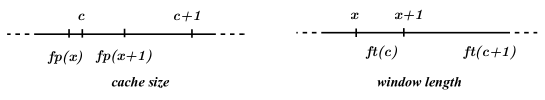
Figure 2: Footprint $\textit{fp}(x)$ and fill time $\textit{ft}(c)$ are inverse functions: $x=\textit{ft}(\textit{fp}(x))$ and $c=\textit{fp}(\textit{ft}(c))$ for all $x,c\geq 0$.

Given cache size $c$ and its fill time $\textit{ft}(c)$, an approximation can be made such that an access is a miss if and only if its reuse time is greater than $\textit{ft}(c)$. The miss ratio is:

$$\textit{mr}(c)=P(rt>\textit{ft}(c))$$ (7)

In theory, Xiang et al. [2013] showed that reuse-time conversion computes the same result as footprint differentiation (Eq. 2.4.1), when the boundary effect is negligible, i.e. for the steady-state footprint (Eq. 4).

In practice, reuse-time conversion has two benefits. First, it counts the cold-start misses correctly. These are first accesses whose reuse time is infinite, since $\textit{rt}>\textit{ft}(c)$ for all $c$. Second, in short traces, e.g. sampled segments, the boundary effect is significant. When it is included, differentiation of the footprint is not guaranteed monotone. Reuse-time conversion, however, guarantees monotone miss ratios.

Sampling makes online analysis possible. For SPEC CPU benchmarks, footprint sampling has been shown to reduce overhead to less than 1% visible Xiang et al. [2013] and less than 0.09 seconds per program on average Wang et al. [2015] and improve accuracy for programs with phase behavior Wang et al. [2015].

A third, theoretical benefit of reuse-time conversion is the justification of an early method by Easton and Fagin.

2.4.3 Easton-Fagin Recipe

Easton and Fagin [1978] were among the first to study cache sharing, in particular, the effect of context switching in cache. They defined a “cold-start cache” as one when a program is switched back and its earlier data have been wiped out, and to distinguish from it, a “warm-start cache” for a regular, solo-use cache.

The 1978 paper gave an ingenious solution to a practical problem: to compute the cold-start miss ratio, which is difficult to simulate, from the miss ratio of warm-start cache, for which simulation is easy. It was ground breaking and pioneered the approach to compute the shared cache performance by reusing the existing solutions already developed for non-shared cache.

Easton and Fagin “gave a rough explanation as to why our recipe is reasonable” but “remarks without proof that this need not be the case, even in the LRU stack model.” However, they found that the “estimate was almost always within 10-15 percent of the directly observed average cold-start miss ratio.” Next we derive the recipe from the measurement theory.

Cache fill time $\textit{ft}(c)$ is the time it takes a program to have the first $c$ misses in cold-start cache of an infinite size. The Easton-Fagin recipe can be written as follows:

$$\textit{ft}(c)\approx\sum_{i=0}^{c-1}\textit{im}(i)$$ (8)

The recipe states that in a cache of size $c$, the fill time is the sum of the inter-miss time in the cache of all smaller sizes. The following formula explains the recipe using the measurement theory

$$\textit{ft}(c)=\sum_{i=0}^{c-1}(\textit{ft}(i+1)-\textit{ft}(i))\approx\sum_{i=0}^{c-1}\textit{im}(i)$$

The preceding formula first rewrites $\textit{ft}(c)$ into a series of sums and then replaces $\textit{mr}(i)$ with the derivative of footprints at the time window of length $\textit{ft}(i)$. The approximation by Easton and Fagin is reduced to the following simpler form:

$$\textit{ft}(i+1)-\textit{ft}(i)\approx\textit{im}(i)=\frac{1}{\textit{mr}(i)}=\frac{\textit{fp}(\textit{ft}(i+1))-\textit{fp}(\textit{ft}(i))}{\textit{fp}(\textit{ft}(i)+1)-\textit{fp}(\textit{ft}(i))}$$

The first two terms show that the derivative of fill time at cache size $i$ is approximated as the inter-miss time at $i$. This approximation is explained in the last term, which is a ratio. The only difference is $\textit{fp}(\textit{ft}(i+1))$ in the enumerator and $\textit{fp}(\textit{ft}(i)+1)$ in the denominator. Both are increases in footprint from the same starting point when the footprint is the cache size $\textit{fp}(\textit{ft}(i))=i$. The denominator is the increase of footprint at $i$ by a unit time, and the enumerator is the increase to fill the cache size $\textit{fp}(\textit{ft}(i+1))=i+1$. This is linear approximation at each $i$ — the rate of footprint increase is constant between $i$ and $i+1$.

Therefore, this section has shown that the Easton-Fagin recipe is a piecewise linear approximation of the footprint. This also explains the flexibility of Easton-Fagin. The granularity of piecewise approximation can be fine, e.g. consecutive cache sizes, or coarse, e.g. power-of-two sizes.

2.4.4 Residence Time

We define the residence time, $\textit{res}(c)$, as the average time a data block stays in cache, from the time of loading into the cache to the time of eviction. The residence time can be computed as follows. Assuming a fully occupied cache of size $c$ for a time period $T$, the sum of residence time of all data blocks is $Tc$, and the number of data blocks loaded in the cache is $T\textit{mr}(c)$. The average residence time is $\textit{res}(c)=\frac{Tc}{T\textit{mr}(c)}=c/\textit{mr}(c)$. The same formula can be derived from the Little’s law $L=\lambda W$, taking the residence time as the service time $W$, the miss ratio as the arrival rate $\lambda$, and the cache size as the average number of customers in a stable system $L$ [Denning and Martell, 2015, pp. 182].

2.5 Linear-time MRC Modeling

A weakness of the Xiang formula (Equation 2.3.2) is that the entire reuse-time histogram is required when computing the footprint of any timescale $x$. The total time to compute the complete footprint $\textit{fp}(x)$ for all timescales is quadratic. This section derives an additive formula of $\textit{fp}(x)$ and then an incremental version of the additive formula that computes the complete footprint $\textit{fp}(x)$ in linear time.

2.5.1 The Additive Formula

To derive an additive formula, we calculate the footprint based on the following observation: if an element $e$ appears more than once in a window, we count only its first appearance in its working-set size.

For a datum $e$, let $\textit{ai}(f_{e})$ be the initial access in the trace. There are three cases:

1. If $f_{e}<w$, $\textit{ai}(f_{e})$ is the first appearance of $e$ in the first $f_{e}$ windows of length $w$.

2. If $w\leq f_{e}\leq n-w+1$, $\textit{ai}(f_{e})$ is the first appearance in $w$ windows of length $w$.

3. If $n-w+1<f_{e}$, $\textit{ai}(f_{e})$ appears first in the last $n-f_{e}+1$ windows of length $w$.

Adding this count for all $e$, we have the total footprint contribution from initial accesses, which we denote as $\textit{fp}_{1}(w)$:

$$fp_{1}(w)=\sum_{f_{e}\leq n-w+1}\min(f_{e},w)+\sum_{f_{e}>n-w+1}(n-f_{e}+1)$$

Next we consider $j$th access ($2\leq j\leq k$) of $e$, i.e., $\textit{ai}(t_{e}^{j})$. There are four cases.

1. If $t_{e}^{j}\leq w$, it is the first appearance in $rt_{e}^{j}$ ($rt_{e}^{j}<w$) windows of length $w$.

2. If $w\leq t_{e}^{j}\leq n-w+1$, it is the first appearance in $\min(rt_{e}^{j},w)$ windows of length $w$.

3. If $t_{e}^{j-1}<n-w+1<t_{e}^{j}$, it is the first appearance in $\min(rt_{e}^{j},w)-(t_{e}^{j}-(n-w+1))$ windows.

4. If $n-w+1\leq t_{e}^{j-1}<t_{e}^{j}$, it is not the first appearance in any window of length $w$, because $\textit{ai}(t_{e}^{j-1})$ and $\textit{ai}(t_{e}^{j})$ always appear together in such windows (the last $n-t_{e}^{j}+1$ windows of length $w$). We express this zero as $rt_{e}^{j}-rt_{e}^{j}$.

We merge all the above terms except the subtractive term in the third and fourth cases. We call the sum $\textit{fp}_{2}(w)$, which can be written concisely as

$$\textit{fp}_{2}(w)=\sum_{i=1}^{n}\min(i,w)\times\textit{rt}(i)$$

We calculate the negative term in the third and fourth case as $\textit{fp}_{3}(w)$. Note that the problem is now isolated since the access $t_{e}^{j}$ lies within the last length-$w$ window, $t_{e}^{j}>n-w+1$. A straightforward solution is to profile the reuse time as before but only for the last $w-1$ accesses, $\textit{ai}(n-w+2\dots n)$. We denote the first and last accesses in the sub-trace by $f_{e}^{\prime}$ and $l_{e}^{\prime}$. For an element $e$, $f_{e}^{\prime}$ equals to $t_{e}^{j}-(n-w+1)$ in the third case. If $f_{e}>n-w+1$, we have $f_{e}^{\prime}=f_{e}-(n-w+1)$ and add $f_{e}-(n-w+1)$ to $\textit{fp}_{3}(w)$. Using the reuse time histogram of the sub-trace, $\textit{fp}_{3}(w)$ can be calculate as:

$$\textit{fp}_{3}(w)=\sum_{i=1}^{w}i\times\textit{rt}^{\prime}(i)+\sum_{e=1}^{m}f_{e}^{\prime}-\sum_{n-w+1<f_{e}}(f_{e}-(n-w+1))$$

We actually do not need to profile again. As a property of the reuse time, we have $\sum\limits_{i=1}^{n-1}i\times\textit{rt}(i)=\sum\limits_{e=1}^{m}(l_{e}-f_{e})$. Then $\textit{fp}_{3}(w)$ equals to:

$$\textit{fp}_{3}(w) = \sum_{e=1}^{m}l_{e}^{\prime}-\sum_{n-w+1<f_{e}}(f_{e}-(n-w+1))$$

$$= \sum_{n-w+1<l_{e}}l_{e}^{\prime}-\sum_{n-w+1<f_{e}}(f_{e}-(n-w+1))$$

$$= \sum_{n-w+1<l_{e}}\left(l_{e}-(n-w+1)\right)-\sum_{n-w+1<f_{e}}(f_{e}-(n-w+1))$$

Putting it all together, the final formula is:

$$(n-w+1)\textit{fp}(w)=\textit{fp}_{1}(w)+\textit{fp}_{2}(w)-\textit{fp}_{3}(w)=wm+\sum_{i=1}^{n}\min(i,w)\times\textit{rt}(i)$$

$$-\sum_{e=1}^{m}d(w-f_{e})-\sum_{e=1}^{m}d\left(l_{e}-(n-w+1)\right)$$ (9)

There is another explanation for the first and the last terms in Equation 2.5.1. $wm$ means that the first access of every element contributes $w$ to the footprint, but for $f_{e}<w$, it only appears in $m-(w-f_{e})$ windows.

The additive formula shows the WS-FP equivalence directly. When $n$ is infinite in the additive formula, all the terms except for $\textit{fp}_{2}$ can be omitted and the additive formula is equivalent to Denning-Schwartz.

2.5.2 The Incremental Formula

We say that a footprint calculation $\textit{fp}(w)$ is incremental if it uses just the part of the reuse histogram $\textit{rt}(i)$ for $i\leq w$. The Xiang formula and the additive method are not incremental because they require the full reuse-time histogram to compute any non-trivial footprint.

To obtain an incremental solution, we start from the initial estimate that every window of size $w$ contains $w$ distinct elements. The maximal sum of working-set sizes is then $(n-w+1)w$. In the following derivation, we divide an access sequence into three parts: the head $\textit{ai}(1\dots w-1)$, the body $\textit{ai}(w\dots n-w+1)$, and the tail $\textit{ai}(n-w+2\dots n)$.

We now decreased the initial estimate $(n-w+1)w$ by removing the duplicates in all windows in each part. Let’s first consider the body and assume that $t_{e}^{j_{1}-1}<w\leq t_{e}^{j_{1}}<\dots<t_{e}^{j_{2}-1}\leq n-w+1<t_{e}^{j_{2}}$ for element $e$. Consider a case where $j$ satisfies $j_{1}\leq j-1<j\leq j_{2}-1$. The two accesses $\textit{ai}(t_{e}^{j-1})$ and $\textit{ai}(t_{e}^{j})$ appear in $d(w-rt_{e}^{j})$ windows. All accesses of $e$ in the body decrease the initial estimate by $d(w-rt_{e}^{j_{1}+1})+\dots+d(w-rt_{e}^{j_{2}-1})$.

In the head sequence, $\textit{ai}(1\dots w-1)$, if $t_{e}^{j-1}<w\leq t_{e}^{j}$, the first $j-2$ accesses duplicate $t_{e}^{1}+t_{e}^{2}+\dots+t_{e}^{j-2}$ times in the first $w$ windows, and the $(j-1)$th access duplicates $d(w-rt_{e}^{j})$ times. Similarly in the tail $\textit{ai}(n-w+2\dots n)$, if $t_{e}^{j-1}\leq n-w+1<t_{e}^{j}$, accesses of $e$ decrease the initial estimate by $d(w-rt_{e}^{j})+(w-t_{e}^{j+1})+\dots+(w-t_{e}^{k})$.

The processing is shown in Algorithm 2 for the head and the tail of a memory trace. The algorithm adds $t_{e}^{i}$ or $(w-t_{e}^{j})$ and subtracts $rt$ in each part. It requires specialized information collection and has no succinct (mathematical) representation except for the algorithm. Given their results as $\textit{lhead},\textit{ltail}$, the complete formula is:

$$(n-w+1)\textit{fp}(w)=(n-w+1)w-\sum_{i=1}^{w-1}(w-i)\textit{rt}(i)+lhead+ltail$$

1

2$\textit{la}(m)\leftarrow\{0\}$;

3for $i=1\textbf{\ to\ }w-1$ do

4       if $\textit{la}(\textit{ai}(i))\neq 0$ then

5             $lhead\leftarrow lhead-\textit{la}(\textit{ai}(i))+(i-\textit{la}(\textit{ai}(i)))$;

6            

7       end if

8      $\textit{la}(\textit{ai}(i))\leftarrow i$;

9      

10 end for

11

12$\textit{la}(m)\leftarrow\{0\}$;

13for $i=n-w+2\textbf{\ to\ }n$ do

14       if $\textit{la}(\textit{ai}(i))\neq 0$ then

15             $ltail\leftarrow ltail-(w-i)+(i-\textit{la}(\textit{ai}(i)))$;

16            

17       end if

18      $\textit{la}(\textit{ai}(i))\leftarrow i$;

19      

20 end for

21

ALGORITHM 2 The Head/Tail Processing of the Incremental Method

To obtain a mathematical description, we use the sub-formula from the additive method to calculate the footprint for windows in the head and tail parts directly.

First, we re-calculate the footprint just for the body part. For each access in $\textit{ai}(w\dots n-w+1)$, we start by assuming that every access contributes $w$ to the footprint and obtain the initial estimate $(n-2w+2)w$. Assume $e$’s reuse time sequence is $t_{e}^{j_{1}-1}<w\leq t_{e}^{j_{1}}<\dots<t_{e}^{j_{2}-1}\leq n-w+1<t_{e}^{j_{2}}$. Based on the previous explanation, the estimate is decreased by $d(w-rt_{e}^{j_{1}+1})+\dots+d(w-rt_{e}^{j_{2}-1})$.

For each access in the head $\textit{ai}(1\dots w-1)$ and tail $\textit{ai}(n-w+2\dots n)$, we use the RT sequence algorithm to traverse either of them and denote the results as $f^{\prime}$,$rt^{\prime}$,$l^{\prime}$ and $f^{\prime\prime}$,$rt^{\prime\prime}$,$l^{\prime\prime}$ respectively. If an element $e$ is accessed in $\textit{ai}(1\dots w-1)$, we have $l_{e}^{\prime}=t_{e}^{j_{1}-1}$. So $\textit{ai}((l_{e}^{\prime}$ contributes $l_{e}^{\prime}-d(w-rt_{e}^{j_{1}})$ to the footprint. Similarly, if $e$ is accessed in $\textit{ai}(n-w+2\dots n)$, and $\textit{ai}(f_{e}^{\prime\prime})$ contributes $(w-f_{e}^{\prime\prime})-d(w-rt_{e}^{j_{2}})$. Let the contributions of the head and the tail be $lhead^{\prime}$ and $ltail^{\prime}$. They can be calculated as:

$$lhead^{\prime} = \sum_{e=1}^{m}l_{e}^{\prime}+\sum_{i=1}^{w-1}(w-i)rt^{\prime}(i)=\sum_{e=1}^{m}f_{e}^{\prime}+w\sum_{i=1}^{w-1}rt^{\prime}(i)$$

$$ltail^{\prime} = \sum_{e=1}^{m}(w-f_{e}^{\prime\prime})+\sum_{i=1}^{w-1}(w-i)rt^{\prime\prime}(i)=w(w-1)-\sum_{e=1}^{m}l_{e}^{\prime\prime}$$

Putting it all together, the incremental method is:

$$(n-w+1)\textit{fp}(w) = (n-2w+2)w-\sum_{i=1}^{w-1}(w-i)\textit{rt}(i)+lhead^{\prime}+ltail^{\prime}$$ (10)

$$= (n+1)m+(n-2m)w-\sum_{i=1}^{w-1}(w-i)\textit{rt}(i)$$

$$+\sum_{e=1}^{m}\min(f_{e},w)-\sum_{e=1}^{m}\max(l_{e},n-w+1)$$

The incremental method computes the footprint in $O(w)$ time and $O(w)$ space. When $w\ll m$, it has a significant advantage in efficiency over all previous solutions.

2.6 Frequency Locality

Frequency is concise — for any $n$ accesses to $m$ data, the average access frequency per datum is $n/m$, a single number.

It is commonly known as “hotness” Chilimbi et al. [1999]; Rubin et al. [2002]. Program data with a greater number of reuses are hotter. The locality is better if the “temperature” is higher. However, the ratio completely ignores the order of data access. The following three traces have the same access frequency but different locality. We name the first two following Denning and Kahn [1975] and the last one following Ding and Kennedy [2004].

cyclic $$: e_{1},e_{2},\dots,e_{m},e_{1},e_{2},\dots,e_{m}$$

sawtooth $$: e_{1},e_{2},\dots,e_{m},e_{m},\dots,e_{2},e_{1}$$

fused $$: e_{1},e_{1},e_{2},e_{2},\dots,\dots,e_{m},e_{m}$$

The locality depends on not just the frequency but also the recency of reuse. Although the three traces reuse the same data, the locality of fused is better than sawtooth, and sawtooth better than cyclic. The closer the reuse is, the better the locality.

In theory, Snir and Yu showed that the complete locality cannot be captured by a fixed size representation Snir and Yu [2005]. One way to measure locality is $\textit{mr}(c)$ for all $c\geq 0$. The Snir-Yu limit implies that the frequency conversion has lost too much information — it is impossible to compute the miss ratio from a fixed number of access frequencies.

Not all locality definitions are equally usable. For the example, the fused sequence has optimal locality, because no other access order can further reduce any reuse distance. This optimality is obvious when analyzed using reuse distance but not using footprint or miss ratio. Since different locality definitions are related, we can now take the optimal locality in one metric, e.g. reuse distance, and derive the optimal values of other metrics, e.g. footprint and miss ratio. The next section presents the complete conversion theory.

2.7 The Complete Theory

Figure 3 shows the MTL graph, where each node is a metric of locality, each directed edge a conversion and, if the edge has a cross ($\times$), the assertion that no such conversion exists. An undirected edge means two directed edge in opposite directions. The MTL conversions are injective. A series of directed edges form a path. The transitive relation gives the conversion or its impossibility between every pair of metrics.

Figure 3: The conversion between the metrics of MTL

The locality metrics are grouped by categories (Figure 1) into six areas in the MTL graph separated by dotted lines. Timescale locality is centrally connected: it is the hub that connects histogram and cache metrics and through them, all metrics.

All the metrics in the MTL graph are from existing work. The contribution of the preceding sections is the connection of these metrics in particular the conversion and non-equivalence results that required for all-to-all relations and were absent from past work.

2.8 Usefulness in Practice

The measurement theory helps to solve problems in practice. The first is precision. All metrics in the MTL graph are defined by mathematics or algorithms. The second is concision and completeness in their relations. A metric may be computed in different ways, and this is shown by multiple paths from the root. Every derivation between two locality concepts is represented by a path in the graph. Each conversion (edge) in the MTL graph is indivisible within itself, i.e. atomic. The third is modularity. A path decomposes a complex construction into individual steps. When there are multiple paths to derive the same metric, their overlap shows shared intermediate concepts and steps. These combinatorial choices are fully expressed but without being enumerated.

Mathematics is not just precise but maintains the precision after many steps of derivation. Furthermore, it proves results for all programs, which are therefore universal. For example, for all programs, it takes linear time to computed the miss ratio of all cache sizes, and the computed miss ratio is bounded and monotone (Theorem 2.14).

Researchers can use multiple metrics when solving a problem. As the example in Section 2.6 shows, it is often convenient to formulate a problem using one metric and solution in another. The measurement theory gives researchers full freedom in using these concepts in practice. Its equivalence and conversion results provide safe bridges, and non-equivalence results mark the boundary and limitations.

3 Related Work

We review more related work in more detail in the following three areas:

Timescale Locality

In 1972, Denning and Schwartz gave a linear-time, iterative formula to compute the average working-set size from reuse times (inter-reference intervals). The derivation was based on stochastic assumptions — that a trace is infinite and generated by a stationary Markov process, i.e. a limit value exists. Later work extended the formula and used it on finite-length traces but did not extend the original theory [Slutz and Traiger, 1974; Denning and Slutz, 1978]. The equivalence theorem (Theorem 2.9) provides a theoretical justification why the Denning-Schwartz formula is accurate without stochastic assumptions.

Shen was the main inventor of a formula that converts from reuse time to reuse distance statistically 2007a. Given the reuse time histogram, the Shen formula predicts the most likely reuse distance histogram. The conversion was 99% accurate and used by the open-source programming tool SLO Beyls and D’Hollander [2006]. The conversion has many steps. It was difficult to understand the reason for its accuracy. The authors actually admitted in the paper that their “formula is hard to interpret intuitively.”

Shen et al. [2007a] defined $p(w)$ as “the probability of any given data element to appear in a time interval of length” $w$ and computed as follows from the reuse time histogram:

$$p(w)=\sum_{i=1}^{w}\sum_{j=i+1}^{n-1}\frac{\textit{rt}(j)}{m-1}$$

If we take the difference $p(w+1)-p(w)$, we see that it is equivalent to the Denning-Schwartz formula divided by $m-1$:

$$p(w+1)-p(w)=\sum_{i=w+2}^{n}\frac{\textit{rt}(i)}{m-1}$$

From footprint, the probability is $p(w)=\textit{fp}(w)/(m-1)$. From its concavity (Corollary 2.13), we can easily prove that $\textit{fp}(w)/m$ is bounded between 0 and 1, as it should being a proper value of probability. The reason for $m-1$ is to model the reuse distance. The reused datum cannot be accessed inside a reuse window. The Shen formula can predict the reuse distance histogram accurately for many applications, which shows the accuracy of timescale locality.

In 2010, Eklov and Hagersten developed Statcache and showed that it was highly accurate (98%) for computer-architecture evaluation. Statcache estimates the average reuse distance $ES(r)$ of all the accesses with the same reuse time $r$. Eklov and Hagersten [2010] defined $F_{j}$ as the fraction of all memory references with a reuse time greater than $j$ and computed the average reuse distance $ES(r)$ using the following formula:

$$ES(r)=\sum\limits_{j=1}^{r}F_{j}=\sum\limits_{j=1}^{r}\sum\limits_{i=j+1}^{n}\textit{rt}(i)$$

The purpose and the method of Statcache are similar to Shen. While the basic formula is identical to Denning-Schwartz, Statcache also developed extremely fast measurement through a novel type of random sampling Eklov and Hagersten [2010]. The subsequent application of Statstack won a best paper award a year later for its efficiency and accuracy Eklov et al. [2011], which are the benefits of using timescale locality to model CPU caches.

The correctness of footprint differentiation was initially validated on the CPU cache Xiang et al. [2011b, 2013]. Three studies since 2014 further evaluated it for fully-associative LRU cache: memory access in data cache Wang et al. [2015], object access in key-value cache, i.e. Memcached Hu et al. [2015], and disk access in server cache Wires et al. [2014]. The three studies re-implemented the footprint analysis independently and reported high accuracy through extensive testing. Hu et al. showed superior speed of convergence using the theory Hu et al. [2015]. Wang et al. showed strong correlation (coefficient 0.938) between the predicted miss ratio and measured co-run speed Wang et al. [2015].

Shared Cache Modeling

Published in 1978, the work of Easton and Fagin was among the first to model the effect of cache sharing due to time sharing. The paper explains the recipe intuitively but “without proof”. Section 2.4.3 derives the recipe mathematically from the measurement theory. A technique to model shared cache is concurrent reuse distance, which shows the locality of a parallel execution precisely but does not have the property of composition as timescale metrics do Schuff et al. [2010]; Wu and Yeung [2013]. Many other techniques are hybrids where the locality is by reuse distance and the interference is by footprint Xiang et al. [2011a]; Chen and Aamodt [2009]; Suh et al. [2001], including one of the first models of multicore cache Chandra et al. [2005]. The relations among these three types of models, footprint, reuse distance, and hybrid, are explained by the measurement theory.

Cache Benchmark Synthesis

Benchmark synthesis is the construction of a synthetic program with desirable locality. It is locality metric conversion in the opposite direction to a trace. Synthesis has been used to solve two practical problems. The first is memory probing with parameterized locality to examine machine performance in multiple use scenarios. APEX-MAP is such a probe program that can be configured so its execution exhibits a distribution of reuse distances similar to a given target [Ibrahim and Strohmaier, 2010]. While APEX-MAP approximates, an algorithm by Shen and Shaw [2008] generates a trace that has the exact reuse distance histogram as specified. The second use of synthesis is black-box benchmark cloning, for which cache behavior cloning is a sub-problem. A system called WEST generates a stochastic trace based on the reuse distance distribution within each cache set, in order to accurately replicate the behavior of set-associative caches Balakrishnan and Solihin [2012].

4 Summary

This paper has formally defined major metrics of locality, grouped them into six categories, and showed a series of relations and properties, including the equivalence between sequence metrics, non-equivalence between histogram metrics, the equivalence between two timescale metrics, a formal justification of the Easton-Fagin recipe, the first solution that computes all miss ratios from the footprint in linear time, and from these results, a complete measurement theory of locality.

APPENDIX

Non-equivalence of Histogram Metrics In the following three theorems, counter examples are used to disprove equivalence.

Theorem A.1.

The memory trace cannot be built from its RT histogram or RD histogram, or the histograms of individual elements.

Proof A.2.

The following two AI traces are different but have the same reuse distance histogram and reuse time histogram for the whole trace and for individual elements:

$$ai : e_{1},e_{2},e_{1},e_{2},e_{2},e_{1}\;\;\;\;\;\;ai^{\prime}:e_{1},e_{2},e_{2},e_{1},e_{2},e_{1}$$

$$rt : \infty,\infty,\;2,\;2,\;1,\;3\;\;\;\;\;\;\;\;rt^{\prime}:\infty,\infty,\;1,\;3,\;2,\;2$$

$$rd : \infty,\infty,\;2,\;2,\;1,\;2\;\;\;\;\;\;\;\;\textit{rd}^{\prime}:\infty,\infty,\;1,\;2,\;2,\;2$$

Theorem A.3.

The RD histogram cannot be built from the RT histogram of the whole trace or individual elements.

Proof A.4.

The following two memory traces produce the same reuse time histogram but different reuse distance histograms, where accesses to $e_{2},e_{4}$ are marked by $\uwave{e_{2}},\uline{e_{4}}$ and the change of their location by $\uuline{e_{2}},\uuline{e_{4}}$:

$$ai : e_{1},\uwave{e_{2}},e_{3},\uline{e_{4}},e_{3},\uuline{e_{4}},e_{1},\uwave{e_{2}},e_{3},\uline{e_{4}},e_{3},\uwave{e_{2}},e_{3},\uuline{e_{2}},e_{3},\uline{e_{4}},e_{3},\uwave{e_{2}},e_{1}$$

$$rt : \infty,\infty,\infty,\infty,\,2,\phantom{{}_{1}}2,\phantom{{}_{1}}6,\phantom{{}_{1}}6,\phantom{{}_{1}}4,\phantom{{}_{1}}4,\phantom{{}_{1}}2,\phantom{{}_{1}}4,\phantom{{}_{1}}2,\phantom{{}_{1}}2,\phantom{{}_{1}}2,\phantom{{}_{1}}6,2,\phantom{{}_{1}}4,12$$

$$rd : \infty,\infty,\infty,\infty,\,2,\phantom{{}_{1}}2,\phantom{{}_{1}}4,\phantom{{}_{1}}4,\phantom{{}_{1}}4,\phantom{{}_{1}}4,\phantom{{}_{1}}2,\phantom{{}_{1}}3,\phantom{{}_{1}}2,\phantom{{}_{1}}2,\phantom{{}_{1}}2,\phantom{{}_{1}}3,2,\phantom{{}_{1}}3,\phantom{{}_{1}}4$$

$$ai^{\prime} : e_{1},\uwave{e_{2}},e_{3},\uline{e_{4}},e_{3},\uuline{e_{2}},e_{1},\uwave{e_{2}},e_{3},\uline{e_{4}},e_{3},\uwave{e_{2}},e_{3},\uuline{e_{4}},e_{3},\uline{e_{4}},e_{3},\uwave{e_{2}},e_{1}$$

$$rt^{\prime} : \infty,\infty,\infty,\infty,\,2,\phantom{{}_{1}}4,\phantom{{}_{1}}6,\phantom{{}_{1}}2,\phantom{{}_{1}}4,\phantom{{}_{1}}6,\phantom{{}_{1}}2,\phantom{{}_{1}}4,\phantom{{}_{1}}2,\phantom{{}_{1}}4,\phantom{{}_{1}}2,\phantom{{}_{1}}2,2,\phantom{{}_{1}}6,12$$

$$rd^{\prime} : \infty,\infty,\infty,\infty,\,2,\phantom{{}_{1}}3,\phantom{{}_{1}}4,\phantom{{}_{1}}2,\phantom{{}_{1}}3,\phantom{{}_{1}}4,\phantom{{}_{1}}2,\phantom{{}_{1}}3,\phantom{{}_{1}}2,\phantom{{}_{1}}3,\phantom{{}_{1}}2,\phantom{{}_{1}}2,2,\phantom{{}_{1}}3,\phantom{{}_{1}}4$$

Theorem A.5.

The RT histogram cannot be built from the RD histogram of the whole trace or individual elements.

Proof A.6.

The following two memory traces produce the same reuse distance histogram but different reuse time histograms:

$$ai : e_{1},e_{2},e_{3},e_{4},e_{3},e_{4},\uuline{e_{1}},\uuline{e_{2}},e_{3},e_{4},e_{3},e_{2},e_{1}$$

$$rt : \infty,\infty,\infty,\infty,\,2,\phantom{{}_{1}}2,\phantom{{}_{1}}6,\phantom{{}_{1}}6,\phantom{{}_{1}}4,\phantom{{}_{1}}4,\phantom{{}_{1}}2,\phantom{{}_{1}}4,12$$

$$rd : \infty,\infty,\infty,\infty,\,2,\phantom{{}_{1}}2,\phantom{{}_{1}}4,\phantom{{}_{1}}4,\phantom{{}_{1}}4,\phantom{{}_{1}}4,\phantom{{}_{1}}2,\phantom{{}_{1}}3,\phantom{{}_{1}}4$$

$$ai^{\prime} : e_{1},e_{2},e_{3},e_{4},e_{3},e_{4},\uuline{e_{2}},\uuline{e_{1}},e_{3},e_{4},e_{3},e_{2},e_{1}$$

$$rt^{\prime} : \infty,\infty,\infty,\infty,\,2,\phantom{{}_{1}}2,\phantom{{}_{1}}5,\phantom{{}_{1}}7,\phantom{{}_{1}}4,\phantom{{}_{1}}4,\phantom{{}_{1}}2,\phantom{{}_{1}}5,11$$

$$rd^{\prime} : \infty,\infty,\infty,\infty,\,2,\phantom{{}_{1}}2,\phantom{{}_{1}}3,\phantom{{}_{1}}4,\phantom{{}_{1}}4,\phantom{{}_{1}}4,\phantom{{}_{1}}2,\phantom{{}_{1}}4,\phantom{{}_{1}}4$$

Appendix B lemma 2.6 to theorem 2.7

$$\sum\limits_{i=1}^{n-1}i\times\textit{rt}(i) = \sum\limits_{e=1}^{m}(l_{e}-f_{e})$$

$$= \sum\limits_{e=1}^{m}(l_{e}-(n-m)+(n-m)-f_{e})$$

$$= (n-m)\times m+\sum\limits_{e=1}^{m}(l_{e}-(n-m))-\sum\limits_{e=1}^{m}f_{e}$$

$$= (n-m)\times m+\sum\limits_{i=1}^{m}i-\sum\limits_{i=1}^{m}i$$

$$= (n-m)\times m$$

Appendix C Eq. (LABEL:eq-nonside) to Eq. (10)

$$(n-w+1)\textit{fp}(w)$$

$$= (n-w+1)m-\sum_{i=w+1}^{n}(i-w)\textit{rt}(i)$$

$$-\sum_{e=1}^{m}d(f_{e}-w)-\sum_{e=1}^{m}d(n-w+1-l_{e})$$

$$= (n-w+1)m-\sum_{i=w+1}^{n}i\times\textit{rt}(i)+w\sum_{i=w+1}^{n}\textit{rt}(i)$$

$$-\sum_{e=1}^{m}d(f_{e}-w)-\sum_{e=1}^{m}d(n-w+1-l_{e})$$

$$= (n-w+1)m-\sum_{i=1}^{n}i\times\textit{rt}(i)+\sum_{i=1}^{w}i\times\textit{rt}(i)$$

$$+w\sum_{i=1}^{n}\textit{rt}(i)-w\sum_{i=1}^{w}\textit{rt}(i)$$

$$-\sum_{e=1}^{m}d(f_{e}-w)-\sum_{e=1}^{m}d(n-w+1-l_{e})$$

$$= (n-w+1)m+\sum_{i=1}^{w}i\times\textit{rt}(i)-w\sum_{i=1}^{w}\textit{rt}(i)$$

$$+w(n-m)-\sum_{e=1}^{m}(l_{e}-f_{e})$$

$$-\sum_{e=1}^{m}d(f_{e}-w)-\sum_{e=1}^{m}d(n-w+1-l_{e})$$

$$= (n+1)m+(n-2m)w-\sum_{i=1}^{w-1}(w-i)\textit{rt}(i)$$

$$+\sum_{e=1}^{m}\min(f_{e},w)-\sum_{e=1}^{m}\max(l_{e},n-w+1)$$

Appendix D Eq. (LABEL:eq-nonside) to Eq. (2.5.1)

$$(n-w+1)\textit{fp}(w)$$

$$= (n-w+1)m-\sum_{i=w+1}^{n}(i-w)\textit{rt}(i)$$

$$-\sum_{e=1}^{m}d(f_{e}-w)-\sum_{e=1}^{m}d(n-w+1-l_{e})$$

$$= (n-w+1)m-\sum_{i=w+1}^{n}(i-w)\textit{rt}(i)$$

$$-\sum_{e=1}^{m}(f_{e}-w)-\sum_{e=1}^{m}(n-w+1-l_{e})$$

$$+\sum_{f_{e}<w}(f_{e}-w)+\sum_{n-w+1<l_{e}}(n-w+1-l_{e})$$

$$= (n-w+1)m-\sum_{i=w+1}^{n}(i-w)\textit{rt}(i)$$

$$+\sum_{e=1}^{m}(l_{e}-f_{e})+mw-m(n-w+1)$$

$$+\sum_{f_{e}<w}(f_{e}-w)+\sum_{n-w+1<l_{e}}(n-w+1-l_{e})$$

$$= w\sum_{i=w+1}^{n}\textit{rt}(i)-\sum_{i=w+1}^{n}i\times\textit{rt}(i)+\sum_{i=1}^{n}i\times\textit{rt}(i)+mw$$

$$+\sum_{f_{e}<w}(f_{e}-w)+\sum_{n-w+1<l_{e}}(n-w+1-l_{e})$$

$$= \sum_{i=1}^{n}\min(i,w)\textit{rt}(i)+mw$$

$$-\sum_{e=1}^{m}d(w-f_{e})-\sum_{e=1}^{m}d(l_{e}-(n-w+1))$$

References

- [1]
- Balakrishnan and Solihin [2012] Ganesh Balakrishnan and Yan Solihin. 2012. WEST: Cloning data cache behavior using Stochastic Traces. In Proceedings of HPCA. 387–398. DOI:http://dx.doi.org/10.1109/HPCA.2012.6169042
- Batson and Madison [1976] A. P. Batson and A. W. Madison. 1976. Measurements of major locality phases in symbolic reference strings. In Proceedings of SIGMETRICS. Cambridge, MA.
- Belady [1966] L. A. Belady. 1966. A study of replacement algorithms for a virtual-storage computer. IBM Systems Journal 5, 2 (1966), 78–101.
- Beyls and D’Hollander [2006] Kristof Beyls and Erik H. D’Hollander. 2006. Discovery of locality-improving refactoring by reuse path analysis. In Proceedings of High Performance Computing and Communications. Springer. Lecture Notes in Computer Science, Vol. 4208. 220–229.
- Buzen [2015] Jeffrey P. Buzen. 2015. Rethinking randomness: a new foundation for stochastic modeling.
- Chandra et al. [2005] Dhruba Chandra, Fei Guo, Seongbeom Kim, and Yan Solihin. 2005. Predicting Inter-Thread Cache Contention on a Chip Multi-Processor Architecture. In Proceedings of HPCA. 340–351.
- Chen and Aamodt [2009] Xi E. Chen and Tor M. Aamodt. 2009. A first-order fine-grained multithreaded throughput model. In Proceedings of HPCA. 329–340.
- Chilimbi et al. [1999] Trishul M. Chilimbi, Bob Davidson, and James R. Larus. 1999. Cache-Conscious Structure Definition. In Proceedings of PLDI. 13–24.
- Denning [1968] Peter J. Denning. 1968. The working set model for program behaviour. Commun. ACM 11, 5 (1968), 323–333.
- Denning [2005] Peter J. Denning. 2005. The locality principle. Commun. ACM 48, 7 (2005), 19–24.
- Denning and Buzen [1978] Peter J. Denning and Jeffrey P. Buzen. 1978. The Operational Analysis of Queueing Network Models. ACM Comput. Surv. 10, 3 (1978), 225–261. DOI:http://dx.doi.org/10.1145/356733.356735
- Denning and Kahn [1975] Peter J. Denning and Kevin C. Kahn. 1975. A study of program locality and lifetime functions. In Proceedings of the ACM Symposium on Operating System Principles. 207–216.
- Denning and Martell [2015] Peter J. Denning and Craig H. Martell. 2015. Great Principles of Computing. MIT Press.
- Denning and Schwartz [1972] Peter J. Denning and Stuart C. Schwartz. 1972. Properties of the working set model. Commun. ACM 15, 3 (1972), 191–198.
- Denning and Slutz [1978] Peter J. Denning and Donald R. Slutz. 1978. Generalized working sets for segment reference strings. Commun. ACM 21, 9 (1978), 750–759.
- Ding and Kennedy [2004] C. Ding and K. Kennedy. 2004. Improving effective bandwidth through compiler enhancement of global cache reuse. J. Parallel and Distrib. Comput. 64, 1 (2004), 108–134.
- Ding et al. [2014] Chen Ding, Xiaoya Xiang, Bin Bao, Hao Luo, Ying-Wei Luo, and Xiao-lin Wang. 2014. Performance Metrics and Models for Shared Cache. J. Comput. Sci. Technol. 29, 4 (2014), 692–712. DOI:http://dx.doi.org/10.1007/s11390-014-1460-7
- Easton and Fagin [1978] Malcolm C. Easton and Ronald Fagin. 1978. Cold-Start vs. Warm-Start Miss Ratios. Commun. ACM 21, 10 (1978), 866–872.
- Eklov et al. [2011] David Eklov, David Black-Schaffer, and Erik Hagersten. 2011. Fast modeling of shared caches in multicore systems. In Proceedings of HiPEAC. 147–157. Best paper.
- Eklov and Hagersten [2010] David Eklov and Erik Hagersten. 2010. StatStack: Efficient modeling of LRU caches. In Proceedings of ISPASS. 55–65.
- Elango et al. [2015] Venmugil Elango, Fabrice Rastello, Louis-Noël Pouchet, J. Ramanujam, and P. Sadayappan. 2015. On Characterizing the Data Access Complexity of Programs. In Proceedings of POPL. 567–580. DOI:http://dx.doi.org/10.1145/2676726.2677010
- Fang et al. [2005] Changpeng Fang, Steve Carr, Soner Önder, and Zhenlin Wang. 2005. Instruction Based Memory Distance Analysis and its Application. In Proceedings of PACT. 27–37.
- Gupta et al. [2013] Saurabh Gupta, Ping Xiang, Yi Yang, and Huiyang Zhou. 2013. Locality principle revisited: A probability-based quantitative approach. JPDC 73, 7 (2013), 1011–1027. DOI:http://dx.doi.org/10.1016/j.jpdc.2013.01.010
- Hong and Kung [1981] J. Hong and H. T. Kung. 1981. I/O complexity: The red-blue pebble game. In Proceedings of the ACM Conference on Theory of Computing. Milwaukee, WI.
- Hu et al. [2015] Xiameng Hu, Xiaolin Wang, Yechen Li, Lan Zhou, Yingwei Luo, Chen Ding, Song Jiang, and Zhenlin Wang. 2015. LAMA: Optimized Locality-aware Memory Allocation for Key-value Cache. In Proceedings of USENIX ATC.
- Hu et al. [2016] Xiameng Hu, Xiaolin Wang, Lan Zhou, Yingwei Luo, Chen Ding, and Zhenlin Wang. 2016. Kinetic Modeling of Data Eviction in Cache. In Proceedings of USENIX ATC.
- Ibrahim and Strohmaier [2010] Khaled Z. Ibrahim and Erich Strohmaier. 2010. Characterizing the Relation Between Apex-Map Synthetic Probes and Reuse Distance Distributions. Proceedings of ICPP 0 (2010), 353–362. DOI:http://dx.doi.org/10.1109/ICPP.2010.43
- Jiang and Zhang [2002] S. Jiang and X. Zhang. 2002. LIRS: an efficient low inter-reference recency set replacement to improve buffer cache performance. In Proceedings of SIGMETRICS. Marina Del Rey, California.
- Lavaee [2016] Rahman Lavaee. 2016. The Hardness of Data Packing. In Proceedings of the 43rd Annual ACM SIGPLAN-SIGACT Symposium on Principles of Programming Languages (POPL 2016). ACM, New York, NY, USA, 232–242.
- Lu and Scott [2011] Li Lu and Michael L. Scott. 2011. Toward a Formal Semantic Framework for Deterministic Parallel Programming. In Proceedings of the International Conference on Distributed Computing. 460–474.
- Marin and Mellor-Crummey [2004] G. Marin and J. Mellor-Crummey. 2004. Cross architecture performance predictions for scientific applications using parameterized models. In Proceedings of SIGMETRICS. 2–13.
- Mattson et al. [1970] R. L. Mattson, J. Gecsei, D. Slutz, and I. L. Traiger. 1970. Evaluation techniques for storage hierarchies. IBM System Journal 9, 2 (1970), 78–117.
- Nugteren et al. [2014] Cedric Nugteren, Gert-Jan van den Braak, Henk Corporaal, and Henri E. Bal. 2014. A detailed GPU cache model based on reuse distance theory. In Proceedings of HPCA.
- Petrank and Rawitz [2002] E. Petrank and D. Rawitz. 2002. The Hardness of Cache Conscious Data Placement. In Proceedings of POPL.
- Rubin et al. [2002] S. Rubin, R. Bodik, and T. Chilimbi. 2002. An efficient profile-analysis framework for data layout optimizations. In Proceedings of POPL. Portland, Oregon.
- Schuff et al. [2010] Derek L. Schuff, Milind Kulkarni, and Vijay S. Pai. 2010. Accelerating multicore reuse distance analysis with sampling and parallelization. In Proceedings of PACT. 53–64.
- Sen and Wood [2013] Rathijit Sen and David A. Wood. 2013. Reuse-based online models for caches. In Proceedings of SIGMETRICS. 279–292.
- Shen and Shaw [2008] Xipeng Shen and Jonathan Shaw. 2008. Scalable Implementation of Efficient Locality Approximation. In Proceedings of the LCPC Workshop. 202–216.
- Shen et al. [2007a] Xipeng Shen, Jonathan Shaw, Brian Meeker, and Chen Ding. 2007a. Locality approximation using time. In Proceedings of POPL. 55–61.
- Shen et al. [2007b] X. Shen, Y. Zhong, and C. Ding. 2007b. Predicting locality phases for dynamic memory optimization. J. Parallel and Distrib. Comput. 67, 7 (2007), 783–796.
- Slutz and Traiger [1974] Donald R. Slutz and Irving L. Traiger. 1974. A Note on the Calculation Working Set Size. Commun. ACM 17, 10 (1974), 563–565. DOI:http://dx.doi.org/10.1145/355620.361167
- Smith [1976] A. J. Smith. 1976. On the Effectiveness of Set Associative Page Mapping and Its Applications in Main Memory Management. In Proceedings of ICSE.
- Snir and Yu [2005] M. Snir and J. Yu. 2005. On the theory of spatial and temporal locality. Technical Report DCS-R-2005-2564. Computer Science Dept., Univ. of Illinois at Urbana-Champaign.
- Suh et al. [2001] G. Edward Suh, Srinivas Devadas, and Larry Rudolph. 2001. Analytical cache models with applications to cache partitioning.. In Proceedings of ICS. 1–12.
- Wang et al. [2015] Wang et al. 2015. Optimal Program Symbiosis in Shared Cache. In Proceedings of CCGrid.
- Wires et al. [2014] Jake Wires, Stephen Ingram, Zachary Drudi, Nicholas JA Harvey, Andrew Warfield, and Coho Data. 2014. Characterizing storage workloads with counter stacks. In Proceedings of OSDI. USENIX Association, 335–349.
- Wu and Yeung [2013] Meng-Ju Wu and Donald Yeung. 2013. Efficient Reuse Distance Analysis of Multicore Scaling for Loop-Based Parallel Programs. ACM Trans. Comput. Syst. 31, 1 (2013), 1. DOI:http://dx.doi.org/10.1145/2427631.2427632
- Wu and Yeung [2011] Meng-Ju Wu and Donald Yeung. 2011. Coherent Profiles: Enabling Efficient Reuse Distance Analysis of Multicore Scaling for Loop-based Parallel Programs. In Proceedings of PACT. 264–275.
- Wu et al. [2013] Meng-Ju Wu, Minshu Zhao, and Donald Yeung. 2013. Studying multicore processor scaling via reuse distance analysis. In Proceedings of ISCA. 499–510.
- Xiang et al. [2011a] Xiaoya Xiang, Bin Bao, Tongxin Bai, Chen Ding, and Trishul M. Chilimbi. 2011a. All-window profiling and composable models of cache sharing. In Proceedings of PPoPP. 91–102.
- Xiang et al. [2011b] Xiaoya Xiang, Bin Bao, Chen Ding, and Yaoqing Gao. 2011b. Linear-time Modeling of Program Working Set in Shared Cache. In Proceedings of PACT. 350–360.
- Xiang et al. [2013] Xiaoya Xiang, Chen Ding, Hao Luo, and Bin Bao. 2013. HOTL: a higher order theory of locality. In Proceedings of ASPLOS. 343–356.
- Zhong et al. [2007] Y. Zhong, S. G. Dropsho, X. Shen, A. Studer, and C. Ding. 2007. Miss rate prediction across program inputs and cache configurations. IEEE Trans. Comput. 56, 3 (March 2007), 328–343.
- Zhong et al. [2009] Yutao Zhong, Xipeng Shen, and Chen Ding. 2009. Program Locality Analysis Using Reuse Distance. ACM TOPLAS 31, 6 (Aug. 2009), 1–39.