Listening to the cohomology of graphs

Abstract.

We prove that the spectrum of the Kirchhoff Laplacian $H_{0}$ of a finite simple Barycentric refined graph and the spectrum of the unimodular connection Laplacian $L$ of $G$ determine each other. Indeed, we note that $L-g$ with $g=L^{-1}$ is similar to the Hodge Laplacian $H=(d+d^{*})^{2}$ of $G$ which is in one dimensions the direct sum $H=H_{0}\oplus H_{1}=d_{0}^{*}d_{0}\oplus d_{0}d_{0}^{*}$ of the Kirchhoff Laplacian $H_{0}$ and its 1-form analog $H_{1}$. In this one-dimensional case, the spectrum of a single choice of one of the three matrices $H_{0},H_{1}$ or $H$ alone is enough to determine both Betti numbers $b_{0},b_{1}$ of $G$ as well as the spectrum of the other matrices. It follows from the similarity of $H$ and $L-L^{-1}$ that for a one-dimensional complex which is a Barycentric refinement, the number of connectivity components $b_{0}$ is the number of eigenvalues $1$ of $L$ and that the genus $b_{1}$ is the number of eigenvalues $-1$ of $L$. It will also lead to much better estimates of spectral radius and algebraic connectivity. For a general abstract finite simplicial complex $G$, we express the Green function values $g(x,y)=\omega(x)\omega(y)\chi({\rm St}(x)\cap{\rm St}(y))$ in terms of the stars ${\rm St}(x)=\{z\in G|x\subset z\}$ of $x$ and $\omega(x)=(-1)^{{\rm dim}(x)}$. One can see $W^{+}(x)=\{z\in G|x\subset z\}$ and $W^{-}(x)=\{z\in G|z\subset x\}$ as stable and unstable manifolds of a simplex $x\in G$ and $g(x,y)=\omega(x)\omega(y)\chi(W^{+}(x)\cap W^{+}(y))$ as heteroclinic intersection numbers or curvatures and the identity $Lg=1$ as a collection of Gauss-Bonnet formulas. A special case is the previously known $g(x,x)=\chi({\rm St}(x))=1-\chi(S(x))$. The homoclinic energy $\omega(x)=\chi(W^{+}(x)\cap W^{-}(x))$ by definition satisfies $\chi(G)=\sum_{x}\omega(x)$. The matrix $M(x,y)=\omega(x)\omega(y)\chi(W^{-}(x)\cap W^{-}(y))$ which is similar to $L(x,y)=\chi(W^{-}(x)\cap W^{-}(y))$ has a sum of matrix entries which is Wu characteristic $\sum_{x\sim y}\omega(x)\omega(y)$. For $G$ with dimension $r\geq 2$ we don’t know yet how to recover the Betti numbers $b_{k}$ from the eigenvalues of the matrix $H$ or from $L$. So far, it is only possible to get it from a collection of block matrices, via the Hodge relations $b_{k}={\rm dim}(H_{k})$. A natural conjecture is that if $G$ is a Barycentric refinement of an other complex, then the spectrum of $L$ determines the Betti vector $b$. This note only shows this to be true if $G$ has dimension $1$.

1. Introduction

1.1.

Any abstract finite simplicial complex $G$ defines a graph $\Gamma=(V,E)$, where $V=G$ and $E$ is the set of pairs of simplices $x,y\in G$, where either $x\subset y$ or $y\subset x$. As the dimension ${\rm dim}:V\to R$ on $\Gamma$ is a coloring, the chromatic number of $\Gamma$ is equal to the clique number ${\rm dim}(G)+1$. The graph $\Gamma$ defines so a new complex $G_{1}$, the Whitney complex of $\Gamma$, which is called the Barycentric refinement of $G$. It consists of all subsets of $V$ in which all elements are connected to each other. The connection matrix $L$ of $G_{1}$ is defined as $L(x,y)=1$ if $x\cap y\neq\emptyset$ and $L(x,y)=0$ else. If ${\rm dim}(G)=1$, then $G_{1}=V\cup E$, with identifying $V$ with $\{\{v\}|v\in V\}$. The connection matrix of $G_{1}$ is then an $n\times n$ matrix, where $n=|G_{1}|=|V|+|E|$.

1.2.

Given a finite abstract simplicial complex $G$ with $f$-vector $(v_{0},v_{1},$ $\dots,$ $v_{r})$, its Dirac operator $D$ is $d+d^{*}$, where $d$ is the exterior derivative $d_{k}f(x_{0},\dots,x_{k})=\sum_{j}(-1)^{j}f(x_{0},\dots,\hat{x}_{j},\dots x_{k})$ from $\Lambda_{k}\to\Lambda_{k+1}$, where $\Lambda_{k}$ is the linear space of antisymmetric functions in $k+1$ variables defined on $k$-dimensional simplices. This space $\Lambda_{k}$ of discrete $k$-forms has dimension $v_{k}$, the cardinality of sets in $G$ of length $k+1$. Also the matrices $d_{k}$ or $D$ can then be realized as $n\times n$ matrices, where $n=\sum_{k=0}^{r}v_{k}$. Both $d$ and so $D$ depend on the orientation chosen for each simplex. (The choice of orientation is a choice of basis in $\Lambda_{d}$ and has nothing to do with orientability as no compatibility is required). The matrix $H=D^{2}$ is the Hodge Laplacian. It decomposes into blocks $H_{k}$, the individual form Laplacians. The kernel of $H_{k}$ has dimension $b_{k}$, which is the $k$’th Betti number. The vector $b=(b_{0},b_{1},\dots,b_{r})$ is the Betti vector of $G$.

1.3.

There are two natural questions: can one read off the Betti vector from the eigenvalues of $L$? Can one read off the Betti vector from the eigenvalues of $H$? We will see that in one dimensions, the two questions are related but that there is already a subtlety: there are $L$-isospectral complexes with different $b_{0},b_{1}$ but that after a Barycentric refinement, we always can read off $b_{0},b_{1}$ from the eigenvalues of $L$. A weaker question is to get the Euler characteristic $\chi(G)=\sum_{k}(-1)^{k}b_{k}$ from the eigenvalues, either in the $L$ or $H$ case. We have seen that one in general can get $\chi(G)$ from the eigenvalues of $L$ as $\chi(G)$ is the number of positive minus the number of negative eigenvalues [15]. In one dimensions, we can get $\chi(G)$ from the eigenvalues of $H$. We don’t know how to get the Euler characteristic $\chi$ from the eigenvalues of $H$ in higher dimensions. We know by Hodge only $\sum_{k}b_{k}$, the nullity of $H$.

1.4.

For one-dimensional complexes, the single incidence matrix $d_{0}$ alone determines everything. The matrix $d_{0}:\Lambda_{0}\to\Lambda_{1}$ is the gradient, its transpose matrix $d_{0}^{*}:\Lambda_{1}\to\Lambda_{0}$ is the divergence. The Hodge Laplacian $H=D^{2}$ has a block decomposition $H=H_{0}\oplus H_{1}$ for $H_{0}=d_{0}^{*}d_{0}$ and $H_{1}=d_{0}d_{0}^{*}$. The matrix $H_{0}=B-A$ is the Kirchhoff matrix of the graph $G$, where $B$ is the diagonal vertex degree matrix and $A$ is the adjacency matrix of $G$. The matrix $H_{1}=d_{1}d_{1}^{*}$ is the Laplacian on $1$-forms. The $0$’th cohomology group $H^{0}(G)$ is defined as ${\rm ker}(d_{0})$, the $1$’st cohomology group $H^{1}(G)$ is the linear space ${\rm ker}(d_{1})/{\rm im}(d_{0})=\mathcal{R}^{m}/{\rm im}(d)$ given by all function on all functions on edges modulo gradients. The nullity $b_{0}$ of $H_{0}$ is the number of connectivity components of $G$. The nullity $b_{1}$ of the matrix $H_{1}$ is the genus of $G$, which is the number of holes or the number of generators of the fundamental group.

1.5.

The operators $L,g=L^{-1}$ and the operators $D,D^{2}=H$ are all defined on the same $n$-dimensional Hilbert space, where $n$ is the number of simplices in $G$. The matrices all depend on the order in which the simplices are arranged. The matrix $D$ also depends on the orientation of simplicial complex. We can not only orient the one and higher dimensional simplices by assigning to them a preferred permutation, allowing to define the orientation through the signature, we can also orient the zero dimensional simplices. This changes $H$ too. In general, the matrix $H$ is always reducible, except if $|G|=1$. On the other hand, the connection operator $L$ is irreducible if $G$ is connected. This means that there is a positive integer $k$ such that $L^{k}$ has only positive entries. Therefore, $L$ has a single Perron-Frobenius eigenvalue and this will be inherited by $H_{0}$.

1.6.

When estimating the largest and smallest non-zero eigenvalue of the Laplacian of a one-dimensional complex it does not matter whether we look for $H_{0},H_{1}$ or $H$. Both the maximal eigenvalue = spectral radius $\rho$ as well as the second eigenvalue = ground state = algebraic connectivity $\alpha$ are of enormous interest. We plan to explore this more elsewhere as in order to appreciate this fully, it requires to compare the improvement with the existing literature on the estimates but a preliminary assessment shows that the formula $H=L-L^{-1}$ is quite powerful to estimate both $\rho$ and $\alpha$ for Barycentric refinement graphs which, all examples of bipartite irregular graphs if $G$ is not circular. (The omission of circular graphs is no issue as we know there all the eigenvalues explicitly). The estimates are often far better than the best established bounds. One of the questions is to estimate how much below the largest eigenvalue has dropped below the obvious upper bound $2d$, where $d$ is the maximal vertex degree of the graph. We can use that $L$ is a non-negative matrix for which much is known [18].

1.7.

The simplest spectral estimate of eigenvalues of $L$ is the upper bound $d_{L}+1$, where $d_{L}$ is the maximal vertex degree of the line graph of $G$, the maximal spectral radius of $H$ is bound above by $d_{L}+1-1/(d_{L}+1)$ which is $\leq 2d-(1/2d)$ if $d$ is the maximal vertex degree. This is better than estimates $2d-2/((2l+1)n)$ ([21] Theorem 3.5) or $2d-1/(ln)$ ([17] Theorem 2.3) established for irregular graphs of diameter $l$ and $n$ vertices. But our new estimate only holds after a Barycentric refinement. But for higher Barycentric refinements we even have $\rho\leq d+2-1/(d+2)$ as the vertex degree of $L$ has then dropped considerably. The relation between $H$ and $L$ is so useful because $L$ is equal o $1+A$, where $A$ is the adjacency matrix of the connection graph of $G$ and $1$ is the identity matrix. The connection graph of $G$ is the graph in which two simplices are connected if they intersect. Any knowledge about the spectrum of adjacency matrices of graphs (like [23]) translates directly into spectral statements of $H$, whether it is spectral radius, algebraic connectivity or order structures of the eigenvalues. The reason is that the map $x\to x-1/x$ maps two spectral intervals of $L$ piecewise monotonically into the spectral interval of $H$.

1.8.

Surprisingly little appears to be known about the relation of the Betti vector $b$ and the eigenvalues $\sigma(H)$ of the Hodge Laplacian, both in the manifold as well as in the case of simplicial complexes. In the graph case, a natural spectral problem is already to relate the spectrum of the adjacency matrix $A$ with the topology of the graph. Its spectrum determines the number of edges and the number of triangles of the eigenvalues of $A$ [2]. For a $2$-dimensional connected complex for which every unit sphere is a $1$-dimensional circular graph $C_{n}$ with $n\geq 4$, we can then read off the Euler characteristic and so the cohomology $\chi(G)=b_{0}-b_{1}+b_{2}=2-b_{1}$ of a connected oriented surface for which the boundary is a collection of closed circular graphs. For the Kirchhoff matrix $B-A$ of a graph, we get the number of vertices, the trace is twice the number of edges from handshaking.

1.9.

We also can get the Zagreb index $z(G)=\sum_{v\in V}{\rm deg}(v)^{2}$ from the spectrum and because $z(G)$ is related to the Wu characteristic $\omega(G)$ we also can get the Euler characteristic. (The connection of Wu characteristic with the Zagreb index has been pointed out to us by Tamas Reti.) This analysis however requires the graph to be geometric, like being a nice triangulation of a $2$-dimensional surface with boundary. To illustrate how little is known, one can ask how to read off the orientability of a triangulated surface from the eigenvalues of the Hodge Laplacian $H$, without indication from which $k$-form vector the zero eigenvalues come from. While non-orientability implies a trivial kernel for the $2$-form Laplacian $H_{2}$, we don’t yet know how to access non-orientability even in the two dimensional from the spectrum of $H=H_{0}\oplus H_{1}\oplus H_{2}$ or from the spectrum of $L$.

2. Relations between spectral data

2.1.

Let us report first a fact which is probably well known even-so we have not found a reference despite the existence of a rather large literature on spectral graph theory. For books, see [2, 7, 6, 3, 4, 19, 22, 5]. As much of this literature is also about spectra of the adjacency matrix, the here discussed relation between $L$ (a shifted adjacency matrix) and $H$ (a Laplacian matrix) is useful as this relation is usually only available for regular graphs, where the vertex degree is constant.

2.2.

In the following, we mean with a graph $G=(V,E)$ the $1$-dimensional simplicial complex $V\cup E$ defined by $G$ and not the Whitney complex. For $G=K_{3}$ for example, this means $G=\{\{1\},\{2\}$, $\{3\},\{1,2\}$, $\{2,3\},\{3,1\}\}$ and not the set of all subsets of $\{1,2,3\}$. In that case, $b_{0},b_{1}$ are determined by the Kirchhoff Laplacian $H_{0}$ alone:

Lemma 1 (Kirchhoff listens to the genus).

For any graph equipped with the 1-dimensional complex, the eigenvalues of the Kirchhoff matrix $H_{0}$ determines the Betti numbers $b_{0},b_{1}$ and the eigenvalues of $H$ as well as the eigenvalues of $H_{1}$. Two $H_{0}$ isospectral graphs are strongly isospectral, meaning $H$-isospectral.

Proof.

By Euler handshake, ${\rm tr}(H_{0})=2|E|$. We also have ${\rm tr}(H_{0}^{0})=|V|$. The number $b_{0}$ is the number of zero eigenvalues of $G$. Now, by Euler-Poincaré, $\chi(G)=b_{0}-b_{1}=|V|-|E|$. From this, one gets

$$b_{1}=b_{0}-|V|+|E|={\rm ker}(H_{0})-{\rm tr}(1)-{\rm tr}(H_{0})/2$$

and the right hand side uses only spectral data. ∎

2.3.

This can be compared with two-dimensional smooth regions in the plane which can be glued together to build a Riemann surface, for which only $b_{0}$ and $b_{1}$ matter. The reason is that we essentially deal with a complex one-dimensional curve then and that the double cover ramified over one-dimensional closed curves is linked to the two dimensional region by Riemann-Hurwitz. So, it is no surprise that one can hear the genus of a drum [8]. We are not aware of any other result, both in the simplicial complex, nor in the manifold case, where one can hear larger Betti numbers $b_{k}(M)$ with $k\geq 2$ from the eigenvalues of any of the Laplacians on a three or higher dimensional manifold without looking at a sequence of form Laplacians $H_{k}$ which build up the Hodge Laplacian $H=\oplus_{k}H_{k}$.

2.4.

In the case of a $1$-dimensional simplicial complex, where are no higher exterior derivatives like the curl $d_{1}$ have to be considered, the spectrum of $H_{0}$ determines completely the spectrum of the Hodge operator $H_{1}$ and so $b_{1}$.

Lemma 2 (Hodge listens to the genus).

Let $H$ be the Hodge matrix of a $1$-dimensional simplicial complex $G$. The eigenvalues of the matrix $H$ alone determine the Betti numbers $b_{0},b_{1}$ of $G$.

Proof.

The matrix $H$ has two blocks $H_{0}=d_{0}^{*}d_{0}=A^{*}A$ and $H_{1}=d_{0}d_{0}^{*}=AA^{*}$. It is a general fact from linear algebra or the Cauchy-Binet formula for the coefficients of the characteristic polynomial [10] that $H_{0}$ and $H_{1}$ are essentially isospectral meaning that their non-zero eigenvalues agree. It is also a very special case of McKean-Singer supersymmetry which in general assures that the non-zero Bosonic and Fermonic spectra agree for the Hodge Laplacian [9]. Now, from $H$, we can access ${\rm ker}(H)=b_{0}+b_{1}$. We can also hear the number of eigenvalues as ${\rm tr}(1)=|V|+|E|$. The trace is ${\rm tr}(H)=2|E|+2|E|=4|E|$. Therefore, we know both $|V|={\rm tr}(1)-{\rm tr}(H)/4$ and $|E|={\rm tr}(H)/4$ and so $\chi(G)=|V|-|E|=b_{0}-b_{1}$. Knowing $b_{0}+b_{1}$ and $b_{0}-b_{1}$ determines $b_{0}$ and $b_{1}$. ∎

2.5.

Lemma 3 (Connection does not hear the genus).

There exist two one-dimensional simplicial complexes which are $L$-isospectral but which have different $b_{0},b_{1}$.

Proof.

The following pair of simplicial complexes was given in [15]. The first one, $G$ is generated by the sets

$$\{\{1,2\},\{1,3\},\{2,6\},\{2,7\},\{6,8\},\{7,4\},\{4,5\}\}$$

The second one is generated by

$$H=\{\{1,2\},\{1,5\},\{1,7\},\{2,8\},\{5,6\},\{8,6\},\{3,4\}\;.$$

∎

2.6.

We know however that in all dimensions, the eigenvalues of $L$ determine the Euler characteristic of $G$ as we have proven that in general, the Euler characteristic $\chi(G)$ is $p(G)-n(G)$, where $p(G)$ and $n(G)$ are the number of positive and negative eigenvalues of the connection Laplacian $L=L(G)$ [15]. In the Barycentric refined case, this will lead to a relation between the eigenvalues $1$ and $-1$ and the Betti numbers. The eigenvectors of $L-L^{-1}$ and $H$ are of course the same.

3. The theorem

3.1.

Our main result here relates the Hodge operator with the “Hydrogen operator” $L-L^{-1}$. The assumption of $G$ having chromatic number $2$ is not that severe but necessary as the above lemma shows. Every Barycentric refinement of a graph has chromatic number $2$, the color being the dimension function.

Theorem 1 (Hydrogen and Hodge).

Given a graph $\Gamma$ which is a Barycentric refinement of a one-dimensional complex, then $L-L^{-1}$ and $H$ are similar. In a suitable basis: $H=L-L^{-1}$.

We will prove this in the next section. The etymology of ”Hydrogren” was explained in [13], where we looked at the functional ${\rm tr}(L-L^{-1})$ which is in general of geometric interest as it is $\sum_{x}\chi(S(x))$. In $\mathcal{R}^{3}$ with Laplacian $L=-\Delta$, the kernel of the inverse $L^{-1}$ is the Newton potential $V_{x}(y)=1/(4\pi|x-y|)$ because of Gauss ${\rm div}{\rm grad}(1/|y-x|)=-4\pi\delta(x)$. In quantum mechanics, the Hydrogen Hamiltonian is $-h^{2}/(2m)\Delta-e^{2}/(4\pi e_{0}r)$ has at least a formal analogy to $L-L^{-1}$.

3.2.

Here is a simple example. We take $G=\{\{1\},\{2\},\{3\},\{1,2\},\{2,3\}\}$ leading to a graph $\Gamma$ with $9$ vertices. It is the simplicial complex $G=\{\{1\},\{2\},\{3\},\{4\},\{5\},\{1,4\},\{2,4\},\{2,5\},\{3,5\}\}$. First, lets write down the connection Laplacian:

$$L=\left[\begin{array}[]{ccccccccc}1&0&0&0&0&1&0&0&0\\ 0&1&0&0&0&0&1&1&0\\ 0&0&1&0&0&0&0&0&1\\ 0&0&0&1&0&1&1&0&0\\ 0&0&0&0&1&0&0&1&1\\ 1&0&0&1&0&1&1&0&0\\ 0&1&0&1&0&1&1&1&0\\ 0&1&0&0&1&0&1&1&1\\ 0&0&1&0&1&0&0&1&1\\ \end{array}\right]\;.$$

The Dirac matrix $D=d+d^{*}$ is

$$D=\left[\begin{array}[]{ccccccccc}0&0&0&0&0&-1&0&0&0\\ 0&0&0&0&0&0&-1&-1&0\\ 0&0&0&0&0&0&0&0&-1\\ 0&0&0&0&0&1&1&0&0\\ 0&0&0&0&0&0&0&1&1\\ -1&0&0&1&0&0&0&0&0\\ 0&-1&0&1&0&0&0&0&0\\ 0&-1&0&0&1&0&0&0&0\\ 0&0&-1&0&1&0&0&0&0\\ \end{array}\right]$$

made of the incidence matrix $d_{0}$, (the lower left block) which is the gradient mapping $0$-forms to $1$-forms as well as its adjoint $d_{0}^{*}$, (the upper right block) which is the divergence mapping $1$-forms to $0$-forms. The Hodge Laplacian $H=D^{2}=(d+d^{*})^{2}$ has now a diagonal block structure $H_{0}\oplus H_{1}$, where $H_{0}$ is the Helmholtz matrix (a $5\times 5$ matrix). The $1$-form block is a $4\times 4$ matrix $H_{1}$ which is essentially isospectral to $H_{0}$. It is an invertible Jacobi matrix in this case, reflecting that $b_{1}=0$:

$$H=\left[\begin{array}[]{ccccccccc}1&0&0&-1&0&0&0&0&0\\ 0&2&0&-1&-1&0&0&0&0\\ 0&0&1&0&-1&0&0&0&0\\ -1&-1&0&2&0&0&0&0&0\\ 0&-1&-1&0&2&0&0&0&0\\ 0&0&0&0&0&2&1&0&0\\ 0&0&0&0&0&1&2&1&0\\ 0&0&0&0&0&0&1&2&1\\ 0&0&0&0&0&0&0&1&2\\ \end{array}\right]\;.$$

The Green’s function is

$$L^{-1}=g=\left[\begin{array}[]{ccccccccc}0&0&0&-1&0&1&0&0&0\\ 0&-1&0&-1&-1&0&1&1&0\\ 0&0&0&0&-1&0&0&0&1\\ -1&-1&0&-1&0&1&1&0&0\\ 0&-1&-1&0&-1&0&0&1&1\\ 1&0&0&1&0&-1&0&0&0\\ 0&1&0&1&0&0&-1&0&0\\ 0&1&0&0&1&0&0&-1&0\\ 0&0&1&0&1&0&0&0&-1\\ \end{array}\right]\;.$$

The Hydrogen operator is the sign-less Hodge matrix. It is a non-negative matrix:

$$L-g=\left[\begin{array}[]{ccccccccc}1&0&0&1&0&0&0&0&0\\ 0&2&0&1&1&0&0&0&0\\ 0&0&1&0&1&0&0&0&0\\ 1&1&0&2&0&0&0&0&0\\ 0&1&1&0&2&0&0&0&0\\ 0&0&0&0&0&2&1&0&0\\ 0&0&0&0&0&1&2&1&0\\ 0&0&0&0&0&0&1&2&1\\ 0&0&0&0&0&0&0&1&2\\ \end{array}\right]\;.$$

The eigenvalues of $H$ are $\sigma(H)=\left\{\right.$ $\frac{1}{2}\left(5+\sqrt{5}\right)$, $\frac{1}{2}\left(5+\sqrt{5}\right)$, $\frac{1}{2}\left(3+\sqrt{5}\right)$, $\frac{1}{2}\left(3+\sqrt{5}\right)$, $\frac{1}{2}\left(5-\sqrt{5}\right)$, $\frac{1}{2}\left(5-\sqrt{5}\right)$, $\frac{1}{2}\left(3-\sqrt{5}\right)$, $\frac{1}{2}\left(3-\sqrt{5}\right)$, $0\left.\right\}$. The eigenvalues of $L$ are $\sigma(L)=\{3.87603$, $2.9563$, $1.90649$, $1.20906$, $1$, $-0.827091$, $-0.524524$, $-0.338261$, $-0.257996$ $\}$. The eigenvalues of $L^{-1}$ are $\sigma(g)=\{-3.87603$, $-2.9563$, $-1.90649$, $-1.20906$, $1$, $0.827091$, $0.524524$, $0.338261$, $0.257996$ $\}$ in accordance to the Zeta function functional equation assuring that $L^{2}$ and $L^{-2}$ have the same eigenvalues if the complex is one-dimensional [16].

3.3.

Using a coordinate change with diagonal matrix $U$ having entries $\omega(x)$ for ${\rm dim}_{G}(x)=0$ and $1$ for ${\rm dim}_{G}(x)=1$, the matrix $H^{+}=UHU^{T}$ is the sign-less Hodge Laplacian. Now, $L-L^{-1}=UHU^{T}=H^{+}$. We have implemented the matrices explicitly using a computer algebra system and included the code at the end. There are many puzzles which remain: we have no idea yet for example how to fix a relation between $L$ and $H$ in the higher dimensional case. We believe that there should be a deformation of $L$ which still makes this happen as we have seen examples, where a change of $L$ works. For a triangle complex $K_{3}$ for example, we just have to change the interaction energy between the $2$-dimensional simplex and the others and still get $H=L-L^{-1}$. Maybe, in general, a small tuning suffices to achieve a connection of $H$ with a non-negative $0-1$ matrix $L$ for which the spectral analysis is easier.

3.4.

As explained below, one can get intuition from physics. The matrix entries can be seen as manifestations of energy potentials. There are indications in the form of examples which suggest that we can change $L$ to still have a Hydrogen formula. This leads to gauge fields. Already the conjugation $H\to UHU^{T}$ is a gauge change even so trivial. It corresponds to a gauge field. The hope is that the inclusion of more general gauge fields (which changes the spectrum of $L$) would allow to save the algebraic relation between $L$ and $H$ also in higher dimensions.

Corollary 1.

For a Barycentric refined graph, the sign-less Hodge matrix $H$ is a non-negative matrix which satisfies $H=L-L^{-1}$ and $H^{2}+2=L^{2}+L^{-2}$.

3.5.

A matrix $A$ is called reducible if there is a basis in which it can be written $A=A_{1}\oplus A_{2}$. If no such decomposition is possible, the matrix is called irreducible. For a non-negative matrix, irreducibility is equivalent to the statement that there exists $k$ such that $A^{k}$ is a positive matrix, meaning that all entries $A^{k}(x,y)$ are positive. Both $H$ and $L$ are non-negative matrices in a suitable basis. If the graph is connected and is not zero-dimensional, then $H$ is reducible but $L$ is irreducible. We can also use that in one dimensions, the spectrum of $L^{2}$ is the same than the spectrum of $L^{-2}$.

Corollary 2.

For a connected Barycentric refined graph, the maximal eigenvalue of the Kirchhoff matrix $H_{0}$ has multiplicity $1$.

3.6.

Example. If $\Gamma=C_{n}$ is a circular graph with even $n$, then $\lambda_{k}=4\sin^{2}(\pi k/n)$ are the eigenvalues of $H=L-L^{-1}$ and $2+16\sin^{4}(\pi k/n)$ are the eigenvalues of $K=H^{2}+2=L^{2}+L^{-2}$. This example was the first time we have seen the relation $H=L-L^{-1}$. It was essential to find an explicit Zeta function of in the Barycentric limit [16].

4. The proof of the theorem

4.1.

In order to prove the result, we need to know the matrix entries of the Green’s function $g=L^{-1}$. We know already the diagonal entries $g(x,x)=1-\chi(S(x))$. This means that for a zero-dimensional simplex $x$, we have $g(x,x)=1-d(x)$, where $d(x)$ is the vertex degree and $g(x,x)=2$ if $x$ is a one-dimensional simplex. Because $L(x,x)=1$, we have $L(x,x)-g(x,x)=d(x)$ on the zero-dimensional sector and $L(x,x)-g(x,x)=2$ for the one-dimensional sector. This matches the matrix entries of $H$ in the diagonal. In order to prove the result we have to establish:

Lemma 4.

a) $g(x,y)=0$ if ${\rm dim}(x)\neq{\rm dim}(y)$ and $x\cap y=\emptyset$.
b) $g(x,y)=1$ if ${\rm dim}(x)\neq{\rm dim}(y)$ and $x\subset y$ or $y\subset x$.
c) $g(x,y)=-1$ if ${\rm dim}(x)={\rm dim}(y)=0$ and $(x,y)\in E$.
d) $g(x,y)=0$ if ${\rm dim}(x)={\rm dim}(y)=1$.

Proof.

We can use this data to build each column vector of $g$. Now just compute the dot product of a $y$ row vector $v$ of $L$ with a $x$ column vector $w$ of $g$ and compute $v\cdot w$. If $x=y$, this is $1$ as there is a hit $1-\chi(S(x))$ and then there are $S(x)$ terms $-1$. For $x\neq y$, then the dot product has only two terms, one being $1$, the other $-1$. Here are a bit more details even so the general case will make this obsolete:
As $G$ is a Barycentric refinement, its vertices are 2-colorable. Any coloring with coloring $0,1$ as well as an orientation of the edges defines a basis. The alternating sign change of the basis assures that $H_{0}^{+}=B+A$ which is the sign-less Kirchhoff matrix. It is isospectral to $H_{0}=B-A$. We will show that $L-L^{-1}=B+A$.
a) First the diagonal: since $H=L-g$, where $g$ is the Green’s operator, we know all the entries of $g$. In the diagonal we have $g(x,x)=1-\chi(S(x))$ $=1-{\rm deg}(x)$. As $L(x,x)=1$, we have $(L-L^{-1}(x,x)=H(x,x)={\rm deg}(x)$. Note that this works also on the 1-form sector as every edge has exactly two neighbors and therefore $(L-L^{-1})(x,x)=1-(1-\chi(S(x))=\chi(S(x))=2$ for an edge.
b) Now the mixed dimension part: assume $x\subset y$ where $x$ is zero dimensional and $y$ is one dimensional. Then we know $L(x,y)=1$ and $L^{-1}(x,y)=\omega(x)=1$. This means that $(L-L^{-1})(x,y)=0$ so that $L-L^{-1}$ has a block structure.
c) Now we look at the case where $x,y$ are both zero dimensional. Then $L(x,y)=0$ and $L^{-1}(x,y)=-1$. This agrees with $H^{+}(x,y)=B+A(x,y)$.
d) Finally look at the case where $x,y$ are both $1$-dimensional. Then $L(x,y)=1$ if $x\cap y$ is not empty and $L(x,y)=0$ else. We can use $L^{-1}(x,y)=0$ to get $(L-L^{-1})(x,y)=1$. Also, if $x,y$ do not intersect, then $L^{-1}(x,y)=0$. ∎

4.2.

The full generalization uses the ”star” ${\rm St}(x)$ of $x$, which is the set of all $y\in G$ if $x\subset y$. It is a collection of simplices, but not a simplicial complex in general. It defines a graph $S^{+}(x)$ in the Barycentric refinement $G_{1}$. There is a subtlety: while we know that for a simplicial complex $G$, the Euler characteristic of $G$ and its Barycentric refinement $G_{1}$ are the same, this is not true for sets of simplices which are not simplicial complexes. Take $A=\{\{1\},\{1,2\}\}$ which is not a simplicial complex but which has Euler characteristic $\chi(A)=\sum_{x\in A}\omega(x)$ with $\omega(x)=(-1)^{{\rm dim}(x)-1}=1-1=0$. The Barycentric refinement $A_{1}$ of $A$ is now the complete graph $K_{2}$ which has Euler characteristic $1$. It is the fact that the star is not a simplicial complex which requires us to compute in $G$ and does not allow us not escape to its Barycentric refinement, which is a graph.

4.3.

The following ”Green star formula” is the ultimate answer about the Green function entries.

Proposition 1 (Green Star formula).

$$g(x,y)=\omega(x)\omega(y)\chi({\rm St}(x)\cap{\rm St}(y))$$

Proof.

(Sketch) We know by Cramer that $g(x,y)={\rm adj}(L)(x,y)/{\rm det}(L)$, where ${\rm adj}(L)$ is the matrix $L$ with row $x$ and column $y$ deleted. Now proceed by induction in the same way as for the unimodularity theorem. For proving the formula for a pair $x,y$, consider an other maximal simplex $z$ away from $x$ and $y$ (which is possible if we don’t deal with a complete graph), then use the multiplicative Poincaré-Hopf formula for the change of the determinant: both sides are multiplied by $1-\chi(S(z))$. See [12]. ∎

4.4.

The Green star formula gives the inverse in a concrete way. One can also write the matrix multiplication $Lg=1$ and verify each entry:

$$\sum_{z}L(x,z)\omega(z)\chi({\rm St}(z)\cap{\rm St}(y))=0$$

if $x\neq y$ and

$$\sum_{z}L(x,z)\omega(z)\chi({\rm St}(z)\cap{\rm St}(x))=\omega(x)\;.$$

Using the notation $z\sim x$ if $x\cap z$ intersect: it means for $x\neq y$

$$\sum_{z\sim x}\omega(z)\chi({\rm St}(z)\cap{\rm St}(y))=0$$

and

$$\sum_{z\sim x}\omega(z)\chi({\rm St}(z)\cap{\rm St}(x))=\omega(x)\;.$$

These are both local Gauss-Bonnet statements similar as in [14]. The Green star formula is equivalent to these two statements about stars in simplicial complexes.

4.5.

Remarks.
1) We have in particular $g(x,x)=\chi({\rm St}(x))$ which means the self-interaction energy of a simplex is the Euler characteristic of its star. 2) If we look at the dual star $W^{-}(x)={\rm St}^{-}(x)$ of $x$, which is the set of all $y\in G$ with $y\subset x$, then this is a complete simplicial complex with Euler characteristic $1$. We can now write

$$L(x,y)=\chi(W^{-}(x)\cap W^{-}(y))\;.$$

We see from this that the matrix $L$ refers to the inside stable part of the simplices while the inverse matrix $g$ refers to the outside unstable part of the simplices.

4.6.

The connection matrix $L$ is conjugated to

$$M(x,y)=\omega(x)\omega(y)\chi(W^{-}(x)\cap W^{-}(y))\;.$$

The inverse $g$ is conjugated via the diagonal matrix ${\rm Diag}(\omega(x))$ to

$$h(x,y)=\chi(W^{+}(x)\cap W^{+}(y))\;.$$

We see an obvious duality. Mending the two pictures requires to go into the complex. Define the diagonal matrix $U$ which has the diagonal entries $U(x,x)=\sqrt{\omega(x)}$. Now we can look at

$$Y=U(L-g)U$$

While $L-g$ is isospectral to the Hodge Laplacian $H=(d+d^{*})^{2}$, the turned operator $Y$ is of the form $H_{0}\oplus(-H_{1})$. Now, paired with the energy theorem $\sum_{x}\sum_{y}g(x,y)=\chi(G)$, we have a relation with the Wu characteristic

$$\omega(G)=\sum_{x,y}L(x,y)\omega(x)\omega(y)$$

which is the total energy of the operator $M$.

Proposition 2.

For any $1$-dimensional complex which is a Barycentric refinement, we have $\sum_{x}\sum_{y}Y(x,y)=\chi(G)-\omega(G)$.

4.7.

Now this is interesting, as the energy is still a combinatorial invariant, a quantity which does not change if we make a Barycentric refinement. We have actually proven in [11], see also [13] that for geometric complexes with boundary, $\chi(G)-\omega(G)=\omega(\delta G)$. If we interpret the curvature for $\chi(G)-\omega(G)$ as an energy of $G$, we see that it is located on the boundary of a complex and that the total energy is zero in the geometric case. For a closed circular graph for example, the total energy of $Y$ is zero. In higher dimensions, the gauge fields have to be added differently and it is still unclear whether one can deform $L$ to mend the Hydrogen formula. If it is possible, then most likely through a variational mechanism which by wishful thinking should relate to some kind of radiation.

Proposition 3.

In general, for any complex $G$, the total energy of $M-g$ is $\chi(G)-\omega(G)$. This total energy is zero for geometric graphs without boundary. The energy curvature is supported on the boundary of a geometric space with boundary.

4.8.

This is not that unfamiliar if we compare a simplicial complex with a space or space time manifold in physics. These manifolds naturally have boundaries as event horizons of singularities. Now, as Hawking famously first pointed out, these boundaries radiate. The analogy is certainly far fetched as what we deal here with relatively basic combinatorial geometry of finite set of sets. Still, it is a mathematical fact that if we define energy of such a geometry as $\chi(G)-\omega(G)$, where $\chi$ is the Euler characteristic and $\omega$ is the Wu characteristic, then due to Dehn-Sommerville, in the interior of Euclidean like parts of space, the energy density (curvature) is zero and all the energy density is at the boundary or located at topological defects of space. History cautions to speculate as the molecular vortex picture debacle reminds. But fundamental questions about the nature of space and time has always motivated mathematics. Here, we deal with remarkable mathematical theorems like the energy theorem which assures that the sum over all interaction energies of simplices in a simplicial complex is the Euler characteristic of the simplicial complex. And this was certainly motivated by physics of the Laplacian in Euclidean space.

4.9.

Let us explain why for any simplicial complex $G$ and any simplex $x\in G$ the ”star formula” $1-\chi(S(x))=\chi({\rm St}(x))$ holds. To see the ”star formula”, we write the unit sphere $S(x)$ as the Zykov join of its stable and unstable part $S(x)=S^{+}(x)+S^{-}(x)$ and use that the ”genus” $i(A)=1-\chi(A)$ is multiplicative $1-\chi(S(x))=(1-\chi(S^{+}(x)))(1-\chi(S^{-}(x)))$. Now, since the stable sphere $S^{-}(x)$ is the boundary of a simplicial complex, we have $1-\chi(S^{-}(x))=\omega(x)=(-1)^{{\rm dim}(x)}$. The statement $(1-\chi(S^{+}(x)))\omega(x)=\chi(St(x))$ is true because every simplex in ${\rm St}(x)$ is bijectively related to a simplex ${\rm St}(x)\setminus x$ in $S(x)$. A vertex $v$ in $S(x)$ corresponds to a simplex $x\cup v$ in $St(x)$. In some sense, collapsing the simplex $x$ in the star ${\rm St}(x)$ to a point and removing that point gives the stable sphere $S^{+}(x)$.

4.10.

The fact that for a bipartite graph, $H_{0}^{+}=B+A$ and the Kirchhoff matrix $H_{0}=B-A$ are unitarily equivalent appears in Proposition 2.2 of [20]. The result more generally holds for completely positive graphs, as these are the graphs which have no odd cycles of length larger than $4$ [1]. It already does not apply for the Barycentric refinemd triangular graph $(K_{3})_{1}$, where the eigenvalues of $H_{0}$ are $\{7,5,4,4,2,2,0\}$ and the eigenvalues of $H_{0}^{+}$ are $\{8,4,4,3,2,2,1\}$.

4.11.

As an application we can compute the eigenvalues of the connection matrices of classes of $1$-dimensional operators like circular graphs. The result also sheds light on the eigenvalue structure. Any integer eigenvalue for $L$ different from $1,-1$ leads to non-integer eigenvalues of $H$. More applications are likely to follow.

5. Hearing the cohomology

5.1.

For a $1$-dimensional complex $G$, the Hodge operator $H=D^{2}$ decomposes into two blocks $H_{0}\oplus H_{1}$. The Betti numbers are then $b_{k}={\rm dim}({\rm ker}(L_{k})$ for $k=0,1$. The $b_{0}$ counts the number of connectivity components, the number $b_{1}$ counts the number of generators of the fundamental group. We in general can not hear the cohomology of a complex, when listening to $L$. The example given is even one-dimensional [15].

5.2.

We assume the complex $\Gamma$ to be a Barycentric refinement of $G$. This implies chromatic number 2 for $\Gamma$ and that $\Gamma$ is bipartite. Lets look first at the eigenvalue $1$:

Lemma 5.

For every connectivity component, we have an eigenvalue $1$ of $L$. The eigenvector is a $\{-1,1\}$-coloring supported on vertices of $\Gamma$ which were zero dimensional in $G$. Every connected component has exactly one eigenvalue $1$.

Proof.

We only have to show that every eigenvector $f$ to an eigenvalue $1$ is supported on vertices of $\Gamma$ which were zero dimensional in $G$. This can be done by induction on the number of $1$-dimensional vertices, (vertices in $\Gamma$ which were $1$-dimensional in $G$). Lets prove more generally that any eigenvector to the eigenvalue $1$ is supported on the $0$-dimensional part of the complex, where it is necessarily a coloring. From the fact that $\sum_{h\sim v,h\in E}f(h)=0$ we get $\sum_{h\in E}f(h)=0$. We can now use induction. Lets call a vertex with vertex degree $1$ a ”leaf”. An eigenvalue $1$ corresponds to an eigenvalue $0$ of the adjacency matrix of the connection graph. For every vertex $v$, the average of all values on edges connected to $v$ is zero. Assume there is an edge $e$ with a leaf attached. Then $f(e)=0$. So, we can apply induction and remove the leaf. Without any leaf, the original complex $G$ must have been a closed loop. Assume that $f(e)>0$ for some $e$. When looking at vertices we see $f(e)$ changes sign along the edges of the loop and that the two neighbors have the same sign and add up to zero. ∎

5.3.

Now, we look at the eigenvalue $-1$:

Lemma 6.

Every homotopically non-trivial closed cycle leads to an eigenvalue $-1$. The eigenvector is a $\{-1,1\}$ coloring of the edges of the cycle and supported on edges. A basis of the eigenspace of $\lambda_{1}$ corresponds to a generating set of the fundamental group.

Proof.

Every cycle leads to an eigenvector: just put alternating values $1,-1$ on the edges of a cycle and put $0$ everywhere else. The fact that every eigenvector can be traced back to a closed path is a consequence of the Hurwicz theorem relating the fundamental group with the first homology group $H^{1}$. The Hurwicz homomorphism is explicit for $H$: take a closed path and build from it a function $f$ on edges telling how many times an edge has been traversed incorporating the direction. Now apply the heat flow $\exp(-tH)$ on this function. As the Hodge matrix $H$ has only nonnegative eigenvalues, the positive eigenvalue part will die out and the limit will be located on the kernel of $H$, which gives a representative of the cohomology group $H^{1}$. It can also be seen from the relation that $L-L^{-1}$ is similar to $H$ as we have already taken care of the eigenvalues $0$ of $H$ which come from eigenvalues $1$ of $L$. and $L-L^{-1}$ has eigenvectors with the same support than $H$ as the conjugation is done by a diagonal matrix. ∎

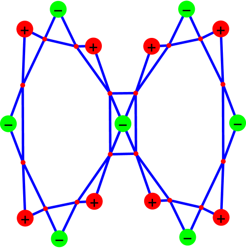
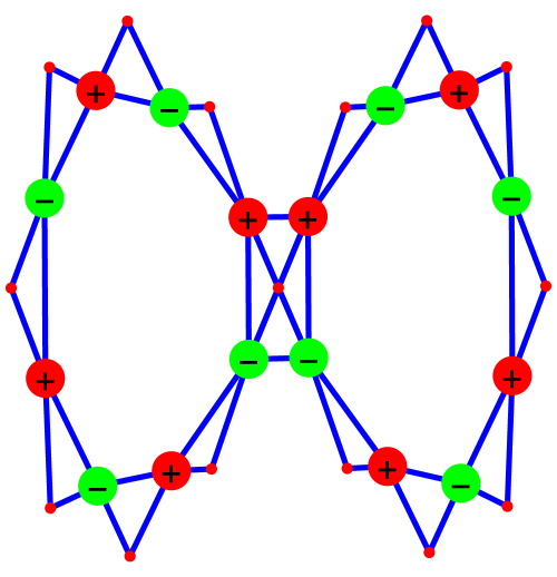
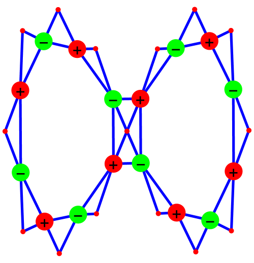
Figure 1. The connection graph $\Gamma^{\prime}$ of the figure 8 graph $G$. It is larger than the Barycentric refinement $\Gamma$ as in the connection graph also edges are connected and has triangles. We see first the eigenvector to the eigenvalue $1$. It is supported on the zero-dimensional parts of the vertex set of $\Gamma$ (the vertices which were $0$-dimensional in $G$). Then we see the two eigenvectors to the two eigenvalues $-1$. They are supported on one-dimensional parts (vertices of $\Gamma$ which were $1$-dimensional in $G$).

5.4.

Can we see from the eigenvalues of $L$, which ones belong to $1$-forms and which one belong to $0$ forms? The positive eigenvalues of $L$ are the ones from the $0$-forms and the negative eigenvalues of $L$ belong to the $1$-forms. For higher dimensional complexes, the eigenvalues of $M=L-L^{-1}$ can take both values. In the one dimensional case, the eigenvalues are always non-negative. We can also describe every point of $H(x,y)$. But in $M(x,y)$, we have connections between vertices and edges, while in $H(x,y)$ we have connections between vertices and vertices, and edges with edges.

5.5.

If $G=G_{1}\times G_{2}$ is the product of two $1$-dimensional complexes which are Barycentric refinements, then the cohomology of $G$ is determined by the cohomology of $G_{i}$. Assume we know the eigenvalues of $G$, we can from the multiplicities get the eigenvalues of $G_{i}$ and so the eigenvalues of the Hodge operators $H_{i}$ and from this the eigenvalues of the Hodge operator $H$ of $G$. Can we do that in general for an arbitrary number of products $G_{i}$?

5.6.

One should probably first focus on the $b_{2}$ case and try to hear the second cohomology $b_{2}$ from the spectrum of $L$. We made some experiments with random complexes and counted the number of different eigenvalues of $H$ and compared this with $b_{2}$. We tried to correlated $b_{2}$ with spectral data like the fraction $\sigma(L)/n$, where $\sigma(G)$ counts the number of different eigenvalues of the $n\times n$ matrix $L$. Also no relation between the factorization of the characteristic polynomial and $b_{2}$ has been found yet. But there are other correlations still to be tried out, like relations between moments ${\rm tr}(L^{k})$ and cohomology or zeta function values with cohomology.

6. Mathematica content

6.1.

Here is an illustration of the Hydrogen formula $H\sim L-L^{-1}$. We take a random graph, refine it to get a one-dimensional complex with chromatic number $2$, then build both $L,H$ and the conjugation diagonal matrix $R$.

⬇

sort[x_]:=Sort[{x[[1]],x[[2]]}]; v=5;e=10; (* size of the graph *)

Gra=RandomGraph[{v,e}]; bracket[x_]:={x}; f={v,e}; q=v+e;

Q=Union[Map[sort,EdgeList[Gra]],Map[bracket,VertexList[Gra]]];

G=Map[bracket,Range[q]]; (* start building Barycentric refinement*)

Do[If[SubsetQ[Q[[k]],Q[[l]]] && k!=l,G=Append[G,{k,l}]],{k,q},{l,q}];

G=Union[Map[Sort,G]]; v=q; n=Length[G];

(* have built now a random Barycentric refined 1-dim complex G *)

Orient[a_,b_]:=Module[{z,c,k=Length[a],l=Length[b]},

If[SubsetQ[a,b] && (k==l+1),z=Complement[a,b][[1]];

c=Prepend[b,z]; Signature[a]*Signature[c],0]];

d=Table[0,{n},{n}]; d=Table[Orient[G[[i]],G[[j]]],{i,n},{j,n}];

Dirac=d+Transpose[d]; H=Dirac.Dirac; (* Hodge Laplacian is built *)

L=Table[If[DisjointQ[G[[k]],G[[l]]],0,1],{k,n},{l,n}];

R=DiagonalMatrix[Table[If[k<=v,(-1)^Length[Q[[k]]],1],{k,n}]];

Total[Flatten[Abs[R.(L-Inverse[L]).R - H]]]

6.2.

We illustrate now the Green star formula

$$g(x,y)=\omega(x)\omega(y)\chi({\rm St}(x)\cap{\rm St}(y))\;.$$

The code computes for an arbitrary simplicial complex the Green’s function entires of the inverse matrix $g=L^{-1}$ of the connection matrix $L$ in terms of the stars ${\rm St}(x)=W^{+}(x)$ and ${\rm St}(y)=W^{+}(y))$. The dimension functional $x\to{\rm dim}(x)$ on $G$ defines a locally injective function which can be seen as a Morse function. The gradient flow of this functional has stable and unstable manifolds $W^{+}(x)$ and $W^{-}(x)$. Speaking in the language of hyperbolic dynamics, the homoclinic tangle of this ”Morse-Smale” system produces the Green functions. Every simplex is a critical point and the definition of Euler characteristic is a special case of the Morse inequality. Indeed, the component $v_{k}$ of the $f$-vector of $G$ counts the number of critical points having Morse index $k$ (The Morse index of a simplex is the dimension of the stable manifold, which is here the $1$ plus the dimension of the sphere $W^{-}(x)\cap S(x)$).

6.3.

The index $\omega(x)=\chi(W^{+}(x)\cap W^{-}(x))$ is related to a homoclinic point, the matrix entries $L(x,y)=\chi(W^{-}(x)\cap W^{-}(y))$ of the connection matrix and the matrix entries $\chi(W^{+}(x)\cap W^{+}(y))$ form the matrix entries of a matrix $RgR^{-1}$ conjugated to the Green’s function, where $R$ is the diagonal matrix with $\omega(x)$ entries. The Wu matrix $M=RLR^{-1}$ is conjugated to $L$ and its matrix entries add up to the Wu characteristic $\omega(G)=\sum_{x\sim y}\omega(x)\omega(y)$.

⬇

Generate[A_]:=Delete[Union[Sort[Flatten[Map[Subsets,A],1]]],1]

Ra[n_,m_]:=Module[{A={},X=Range[n],k},Do[k:=1+Random[Integer,n-1];

A=Append[A,Union[RandomChoice[X,k]]],{m}];Generate[A]];

G=Ra[7,15];n=Length[G];SQ=SubsetQ; OmegaComplex[x_]:=-(-1)^Length[x];

EulerChiComplex[GG_]:=Total[Map[OmegaComplex,GG]];

S[x_]:=Module[{u={}},Do[v=G[[k]];If[SQ[v,x],u=Append[u,v]],{k,n}];u];

K=Table[OmegaComplex[G[[k]]] OmegaComplex[G[[l]]],{k,n},{l,n}];

H=Table[Intersection[S[G[[k]]],S[G[[l]]]],{k,n},{l,n}];

h = Table[K[[k, l]] EulerChiComplex[H[[k, l]]], {k, n}, {l, n}];

L=Table[If[DisjointQ[G[[k]],G[[l]]],0,1],{k,n},{l,n}];

h.L==IdentityMatrix[n]

References

- [1] A. Berman. Completely positive graphs. In S. Friedland R.A. Brualdi and V. Klee, editors, Combinatorial and Graph Theoretical Problems in Linear Algebra, pages 228–233. Springer Verlag, 1993.
- [2] N. Biggs. Algebraic Graph Theory. Cambridge University Press, 1974.
- [3] A.E. Brouwer and W.H. Haemers. Spectra of graphs. Springer, 2012.
- [4] F. Chung. Spectral graph theory, volume 92 of CBMS Regional Conf. Series. AMS, 1997.
- [5] D. Cvetkovic, P. Rowlinson, and S. Simic. An Introduction to the Theory of Graph Spectra. London Mathematical Society, Student Texts, 75. Cambridge University Press, 2010.
- [6] M. Doob D. Cvetković and H. Sachs. Spectra of graphs. Johann Ambrosius Barth, Heidelberg, third edition, 1995. Theory and applications.
- [7] Y.Colin de Verdière. Spectres de Graphes. Sociéte Mathématique de France, 1998.
- [8] M. Kac. Can one hear the shape of a drum? Amer. Math. Monthly, 73:1–23, 1966.
-
[9]
O. Knill.
The McKean-Singer Formula in Graph Theory.
http://arxiv.org/abs/1301.1408, 2012. - [10] O. Knill. A Cauchy-Binet theorem for Pseudo determinants. Linear Algebra and its Applications, 459:522–547, 2014.
-
[11]
O. Knill.
Gauss-Bonnet for multi-linear valuations.
http://arxiv.org/abs/1601.04533, 2016. -
[12]
O. Knill.
On Fredholm determinants in topology.
https://arxiv.org/abs/1612.08229, 2016. -
[13]
O. Knill.
On a Dehn-Sommerville functional for simplicial complexes.
https://arxiv.org/abs/1705.10439, 2017. -
[14]
O. Knill.
On Helmholtz free energy for finite abstract simplicial complexes.
https://arxiv.org/abs/1703.06549, 2017. -
[15]
O. Knill.
One can hear the Euler characteristic of a simplicial complex.
https://arxiv.org/abs/1711.09527, 2017. -
[16]
O. Knill.
An elementary Diadic Riemann hypothesis.
https://arxiv.org/abs/1801.04639, 2018. - [17] J. Li, W.C. Shiu, and W.H. Chan. The Laplacian spectral radius of graphs. Czechoslovak Mathematical Journal, 60:835–847, 2010.
- [18] H. Minc. Nonnegative Matrices. John Wiley and Sons, 1988.
- [19] P.VanMieghem. Graph Spectra for complex networks. Cambridge University Press, 2011.
- [20] R. Merris R. Grone and V.S. Sunder. The Laplacian spectrum of a graph. SIAM J. Matrix Anal. Appl., 11(2):218–238, 1990.
- [21] L. Shi. Bounds of the Laplacian spectral radius of graphs. Linear algebra and its applications, pages 755–770, 2007.
- [22] D.A. Spielman. Spectral graph theory. lecture notes, 2009.
- [23] D. Stevanovic. Spectral Radius of Graphs. Elsevier, 2015.