Multidimensional Data Driven Classification of blackEmission-line Galaxies

Abstract

We propose a new soft clustering scheme blackfor classifying galaxies in different activity classes using simultaneously 4 emission-line ratios; $\log($[N ii]$/$H$\alpha$), $\log$([S ii]$/$H$\alpha$), $\log$([O i]$/$H$\alpha$) and $\log$([O iii]$/$H$\beta$). We fit black20 multivariate Gaussian distributions blackto the 4-dimensional distribution of these lines obtained from the Sloan Digital Sky Survey (SDSS) in order to capture local structures and subsequently group the multivariate Gaussian distributions blackto represent the complex multi-dimensional structure of the joint distribution of galaxy spectra in the 4 dimensional line ratio space. blackThe main advantages of this method are the use of all four optical-line ratios simultaneously and the adoption of a clustering scheme. This maximises the use of the available information, avoids contradicting classifications, and treats each class as a distribution resulting in soft classification boundaries blackand providing the probability for an object to belong to each class. We also introduce linear multi-dimensional decision surfaces using support vector machines blackbased on the classification of our soft clustering scheme. This linear multi-dimensional hard clustering technique shows high classification accuracy with respect to our soft-clustering scheme.

1 Introduction

blackThe production of electromagnetic radiation in galaxies is dominated by two main processes: star-formation and/or accretion onto a supermassive central black-hole, the latter witnessed as an Active Galactic Nucleus (AGN). The blackcharacterization of these processes and the study of their interplay is key for understanding the demographics of galactic activity and the co-evolution of nuclear black-holes and their host galaxies (e.g. Kormendy & Ho, 2013). blackOne of the most commonly used tools for characterising the type of activity in galaxies is its imprint on the emerging spectrum of the photoionised interstellar medium (ISM). AGN generally produce harder ionising continua which result in spectra with stronger high-excitation lines black compared to the spectra we can obtain from photoionization by young stellar populations (e.g. Ferland, 2003).

The importance of characterising the ionising source of emission-line regions was recognised early on and led to the first systematic presentation of optical emission-line diagnostic tools by Baldwin, Phillips & Terlevich (1981). This work introduced two-dimensional diagrams involving the ratios of various optical emission lines (e.g. $[\text{Ne\,{v}}]$ $\mathrm{\lambda 3426\AA}$, $[\text{O\,{ii}}]$ $\mathrm{\lambda 3727\AA}$, $[\text{O\,{iii}}]$ $\mathrm{\lambda 5007\AA}$, $[\text{O\,{i}}]$ $\mathrm{\lambda 6300\AA}$, $[\text{N\,{ii}}]$ $\mathrm{\lambda 6584}$ He ii $\mathrm{\lambda 4686\AA}$, H$\alpha$, and H$\beta$) that can separate emission-line regions excited by stellar photoionizing continuum, power-law photoionizing continuum, or shocks. Therefore, these diagrams, known as Baldwin-Phillips-Terlevich (BPT) diagrams, were able to discriminate between star-forming galaxies (SFGs) and galaxies dominated by AGN activity. At the same time, a third class of galaxies was recognized by Heckman (1980) on the basis of their relatively stronger lower-ionisation lines (Low-Ionisation Nuclear Emission line Regions; LINERs). The format of the BPT diagrams that are typically used today was refined by Veilleux & Osterbrock (1987) to involve the $\log$([O iii]$\mathrm{\lambda 5007\AA}/$H$\beta$) emission-line intensity ratios plotted against one of the $\log($[N ii]$\mathrm{\lambda 6584}/$H$\alpha$), $\log$([S ii]$\mathrm{\lambda\lambda 6716,6731}/$H$\alpha$), $\log$([O i]$\mathrm{\lambda 6300}/$H$\alpha$) emission-line intensity ratios, and they can discriminate between all three classes of objects (SFGs, LINERs, AGN).

blackHowever, the exact demarcation between SFGs and AGNs is generally defined empirically and hence it is subject to considerable uncertainty. Based on stellar population synthesis and photoinization models Kewley et al. (2001) introduced a maximum ’starburst’ line on the BPT diagrams which defines the upper bound for the SFGs. Driven by the fact that AGN and SFGs observed in the Sloan Digital Sky Survey (SDSS; York et al. 2000) show two distinct loci extending below the demarcation line of Kewley et al. (2001), a new empirical upper bound for the SFGs was put forward by Kauffmann et al. (2003) in order to distinguish the pure SFGs. The objects between this new empirical SFG line and the demarcation line of Kewley et al. (2001) belong to the class of Composite galaxies (also referred to as Transition objects in previous studies; e.g. Ho et al. 1997). blackThe spectra of these Composite galaxies have been traditionally interpreted as the result of significant contributions from both AGN and star-forming activity, although, more recently it has been proposed that their strong high-excitation lines could be the result of shocks (e.g. Rich et al., 2014). blackBased on the density of the objects in the 2-dimensional diagnostic diagrams, Kewley et al. (2006) introduced another empirical line for distinguishing Seyferts and LINERs. More recently, Shi et al. (2015) blackexplored other emission-line intensity ratios blackthat could improve the classification. They used support vector machines to test the classification accuracy using a dataset of galaxies classified as either SFG, AGN, or Composite based on Kauffmann et al. (2003).

The currently used classification scheme suffers from blacka significant drawback. The use of multiple diagnostic diagrams independently of one another often gives contradicting classifications for the same galaxies (e.g. Ho et al., 1997). According to Kewley et al. (2006), $8\%$ of the galaxies in their sample are characterised as ambiguous in that they were classified as blackbelonging to different classes blackbased on at least two diagnostic blackdiagrams. blackFor clarity, blackthroughout this paper, we use the term contradicting to emphasise that the different 2-dimensional diagnostics can give different classifications. blackSuch blackcontradictions arise because BPT diagrams are projections of a complex multi-dimensional space onto 2-dimensional planes. This limits the power of blackthis diagnostic tool and may lead to inconsistencies between the different diagnostic diagrams. Moreover, the number of extragalactic emission-line objects for which accurate spectra are available has grown rapidly in recent years, especially with the advent of the SDSS. This massive dataset reveals inconsistencies between the theoretical and empirical upper bounds and the actual distribution of the observed line ratios for the different classes (e.g. Kauffmann et al., 2003).

This limitation of the existing approach gives rise to the question of whether we can use a multidimensional data-driven method to effectively classify the galaxies. Recently, Vogt et al. (2014), generalised the diagnostics originally proposed by Kewley et al. (2006) by providing multi-dimensional surfaces blackin different groups of diagnostic lines that separate different activity classes. These, however, do not include the standard BPT diagnostic ratios. blackSimilarly, de Souza et al. (2017) explore the use of Gaussian mixture models for the activity classification of galaxies in the 3-dimensional parameter space defined by the [O iii]$/$H$\beta$, [N ii]$/$H$\alpha$, line ratios and the H$\alpha$ equivalent width (EW(H$\alpha$)).

In this article we propose a classification scheme, the soft data-driven allocation (SoDDA) method, which is based on the clustering of galaxy emission-line ratios in the 4-dimensional space defined by the [O iii]$/$H$\beta$, [N ii]$/$H$\alpha$, [S ii]$/$H$\alpha$, and [O i]$/$H$\alpha$ ratios. This is motivated by the clustering of the SFG, AGN, and LINER loci on the 2D projections of the emission-line diagnostic diagrams. Our classification scheme arises from a model that specifies the joint distribution of the emission-line ratios of each galaxy class to be a finite mixture of multivariate Gaussian (MG) distributions. Given the emission line ratios of each galaxy, we compute its posterior probability to belong to each galaxy class. This allows us to achieve a soft clustering blackwithout hard separating boundaries between the different classes. A similar approach was successfully implemented by Mukherjee et al. (1998) in another clustering problem in which they used a mixture of MG distributions blackto discriminate between distinct classes of gamma-ray bursts.

This paper is organised as follows. In Section 2 we describe the proposed methodology. Section 3 discusses the implementation of the method on galaxy spectra from the SDSS DR8, and Section 4 compares our multidimensional data driven classification scheme with the blackcommonly used diagnostic proposed by Kewley et al. (2006). Section 5 introduces multidimensional linear decision boundaries that we compare in terms of their prediction accuracy with both the SoDDA and the scheme of Kewley et al. (2006). In Section 6 we review our results and discuss further research directions.

2 Clustering Analysis

Cluster analysis is a statistical method that aims to partition a dataset into subgroups so that the members within each subgroup are more homogeneous (according to some criterion) than the population as a whole. In this article we employ a class of probabilistic (model-based) algorithms that assumes that the data are an identically and independently distributed (i.i.d.) sample from a population described by a density function, which is taken to be a mixture of component density functions. Finite mixture models have been studied extensively as a clustering technique (Wolfe, 1970). It is common to assume that the mixture components are all from the same parametric family, such as the Gaussian. The use of mixture models arises naturally in our problem, since the population of galaxies is made up of several homogeneous blackand often overlapping subgroups blackfrom a spectroscopic perspective: SFGs, Seyferts, LINERs and Composites.

Fraley & Raftery (2002) proposed a general framework to model a population as a mixture of $K$ subpopulations. Specifically, let $x_{i}$ be a vector of length $p$ containing measurements of object $i$ ($i=1,...,n)$ from a population. In our application the $x_{i}$ tabulates the $p=4$ emission line ratios for galaxy $i$. A finite mixture model expresses the likelihood of $x_{i}$ as:

$$p(x_{i}|\theta,\pi)=\sum_{k=1}^{K}\pi_{k}f_{k}(x_{i}|\theta_{k}),$$ (1)

where $f_{k}$ and $\theta_{k}$ are the probability density and parameters for the distribution of subpopulation $k$, and $\pi_{k}$ is the relative size of subpopulation $k$, with $\pi_{k}\geq 0$ and $\sum_{i=1}^{K}\pi_{k}=1$. Given a sample of n independent galaxies $x=(x_{1},x_{2},...,x_{n})$, the joint density can be expressed as:

$$p(x|\theta,\pi)=\prod_{i=1}^{n}\sum_{k=1}^{K}\pi_{k}f_{k}(x_{i}|\theta_{k}),$$ (2)

where $\theta=(\theta_{1},...,\theta_{K})$ and $\pi=(\pi_{1},...,\pi_{K})$.

2.1 Estimating the parameters of a finite mixture model

Dempster, Laird & Rubin (1977) propose a framework that can be used to compute the maximum likelihood estimators (MLE) in finite mixture models using the Expectation-Maximization (EM) algorithm. blackWe blackdenote the unknown parameters as $\phi=(\theta,\pi)$. The MLE is $\phi^{\star}=\text{argmax}_{\phi}p(x\mid\phi)$, where argmax_ϕ is an operator that extracts the value of $\phi$ that maximises the likelihood function, $p(x\mid\phi)$. The EM algorithm is an iterative method for computing the MLE.

In the context of finite mixture models, Dempster et al. (1977) introduced an unobserved vector $z$ ($n\times K$), where $z_{i\bullet}$ is the indicator vector of length $K$ with $z_{ik}=1$ if object $i$ belongs to subpopulation $k$ and $0$ otherwise. Because the $z_{i\bullet}$ are not observable, they are called latent variables. In this case they specify to which subpopulation each galaxy belongs. Given a statistical model consisting of observed data $x$, a set of unobserved latent data $z$, and a vector of unknown parameters $\phi=(\theta,\pi)$, the EM algorithm iteratively performs alternating expectation (E) and maximisation (M) steps:
E-step: Compute $Q(\phi|\phi^{(t)})=\text{E}[\log\>p(x,z|\phi)|x,\phi^{(t)}]$,

M-step: Set $\phi^{(t+1)}=\text{argmax}_{\phi}\>Q(\phi|\phi^{(t)})$,

where the superscript $t$ indexes the iteration, and E[.] is the weighted mean evaluated by marginalising over all possible values of $z$. The EM algorithm enjoys stable convergence properties, in that the likelihood, $p(x|\phi)$, increases in each iteration and the algorithm is known to converge to a stationary point of $p(x|\phi)$, which is typically a local maximum.

The joint distribution $p(x,z|\theta,\pi)$ can be factorised as $p(x,z|\theta,\pi)=p(z|\theta,\pi)p(x|z,\theta,\pi)$, where $p(z|\theta,\pi)$ is a product of $n$ multinomial distribution $p(z|\theta,\pi)=\prod_{i=1}^{n}\prod_{k=1}^{K}\pi_{k}^{z_{ik}}$. Conditional on $z_{ik}=1$, $p(x_{i})=f_{k}(x_{i}|\theta_{k})$. The logarithm of the conditional distribution of $x$ and $z$ given $(\theta,\pi)$, i.e. the log-likelihood, is:

$$\ell(\theta,\pi|x,z)=\log p(x,z\mid\theta,\pi)=\sum_{i=1}^{n}\sum_{k=1}^{K}z_{ik}\log[\pi_{k}f_{k}(x_{i}|\theta_{k})].$$ (3)

The E-step requires us to compute the conditional expectation of Equation 3 given $(\theta^{(t)},\pi^{(t)})$. Because Equation 3 is linear in the components of each $z_{i\bullet}$, it suffices to compute the conditional expectation of the components of each $z_{i\bullet}$ given $x$ and $(\theta^{(t)}$, $\pi^{(t)})$. This is the conditional probabilities of $i$ belonging to subpopulation $k$ given $(\theta^{(t)}$, $\pi^{(t)})$. More specifically:

$$\text{E}[z_{ik}|\theta^{(t)},\pi^{(t)},x]=\frac{\pi_{k}^{(t)}f_{k}(x_{i}|\theta_{k}^{(t)})}{\sum_{k=1}^{K}\pi_{k}^{(t)}f_{k}(x_{i}|\theta_{k}^{(t)})}=\gamma(z_{ik})$$ (4)

The M-step requires us to maximise the conditional expectation of Equation 3 with respect to $\pi$ and $\theta$, i.e. to maximise $\sum_{i=1}^{n}\sum_{k=1}^{K}\gamma(z_{ik})\log[\pi_{k}f_{k}(x_{i}|\theta_{k})]$. The particular form of the M-step depends on the choice of density distributions, $f_{k}$, for the subpopulations. Here we assume MG distributions for each subpopulation.

MG mixture models can be used for data with varying structures due to the flexibility in the definition of variance matrices. The density of the MG distribution for subpopulation $k$ is:

$$f_{x}(x_{i})=\frac{1}{\sqrt{(2\pi)^{p}|\Sigma_{k}|}}\exp\Big{(}-\frac{1}{2}(x_{i}-\mu_{k})^{T}\Sigma_{k}^{-1}(x_{i}-\mu_{k})\Big{)}.$$ (5)

The EM formulation for an MG mixture is presented in detail in Dempster et al. (1977). The E-step has the same formulation as in Equation 4, with $f_{k}$ given in Equation 5 with $\theta_{k}=(\mu_{k},\Sigma_{k})$, where $\mu_{k}$ represent the means and $\Sigma_{k}$ the covariance matrices of the $x_{i}$ line ratios for galaxies in subpopulation $k$. For the M-step, the updates of the parameters have closed form solutions (Bilmes et al., 1998),

$$\pi_{k}^{(t+1)} =\frac{1}{n}\sum_{i=1}^{n}\gamma(z_{ik})$$ (6)

$$\mu_{k}^{(t+1)} =\frac{\sum_{i=1}^{n}x_{i}\gamma(z_{ik})}{\sum_{i=1}^{n}\gamma(z_{ik})}$$ (7)

$$\Sigma_{k}^{(t+1)} =\frac{\sum_{i=1}^{n}\gamma(z_{ik})(x_{i}-\mu_{k}^{(t+1)})(x_{i}-\mu_{k}^{(t+1)})^{T}}{\sum_{i=1}^{n}\gamma(z_{ik})}.$$ (8)

We implement this EM algorithm using the scikit-learn Python library under the constraint that the covariance matrices are full rank, and the diagonal elements cannot be smaller than $10^{-3}$ to avoid overestimation, i.e. converging to a small number of data points. Because this algorithm can be sensitive to the choice of starting values, we routinely rerun it with 5 different randomly selected sets of starting values. blackThe values of the likelihood for the different starting values differ less than $0.5\%$. We choose the value among the 5 converged points with the largest likelihood to be the MLE, denoted $(\pi^{\star},\mu^{\star},\Sigma^{\star})$.

2.2 Choosing the value of $K$

Fraley & Raftery (2002) point out that mixtures of MG distributions are appropriate if the subpopulations are centred at the means, $\mu_{k}$, with increased density for data closer to the means. As a result, the practical use of MG mixture models could be limited if the data exhibit non-Gaussian features, including asymmetry, multi-modality and/or heavy tails. In the SDSS blackDR8 dataset that we examine, it is apparent that the subpopulations exhibit non Gaussians characteristics such as convexity, skewness and multimodality. In order to account for these non-Gaussian features, we use a mixture of MG distributions with $K$ considerably larger than the actual number of galaxy classes. In this way, we represent each galaxy class by a mixture of several MG subpopulations. This allows a great deal of flexibility in the class-specific distributions of emission line ratios. With the fitted (large $K$) MG mixture in hand we can then perform hyper-clustering of the $K$ MG subpopulations so as to concatenate them into clusters representing the four desired galaxy classes.

The number $(K>>4)$ of MG subpopulations that we fit to our data is chosen using the Bayesian Information Criterion (BIC) of Schwarz et al. (1978) and the gap statistic (Tibshirani et al., 2001). BIC is a model selection criterion based on the maximum log-likelihood obtained with each possible value of $K$, and penalised by the increased complexity associated with more subpopulations . More specifically, it is defined as $\text{BIC}(K)=-2\cdot L^{\star}(K)+K\log(n)$, where $L^{\star}(K)=p(x\mid\theta^{\star}(K),\pi^{\star}(K))$ is the maximised value of the likelihood when the number of subpopulations is fixed at $K$. The value of $K$ with the lowest BIC is preferred. The gap statistic compares the normalised intra-cluster distances between points in a given cluster, $W_{K}$, for different total number of subpopulations $K$, with a null reference distribution obtained assuming data with no obvious clustering. The null reference distribution is generated by sampling uniformly from the original datasets bounding box multiple times. The estimate for the optimal number of subpopulations $K$ is the value for which the $W_{K}$ falls the farthest below the reference curve.

SoDDA accomplishes the hyper-clustering of the $K$ subpopulations into the four galaxy classes using the classification scheme of Kewley et al. (2006). More specifically, we treat the fitted subpopulations means $(\mu_{1}^{\star},...,\mu_{K}^{\star})$ as a dataset and classify them into the four galaxy classes. For example, suppose we fit 10 MG distributions and the means of the distributions $1,3$ and $5$ are classified by Kewley et al. (2006) as SFGs, then the distribution of the SFGs under SoDDA would be

$$f_{\text{SFG}}(x_{i})=\frac{\pi_{1}^{\star}f_{1}(x_{i}|\theta_{1}^{\star},\pi_{1}^{\star})+\pi_{3}^{\star}f_{3}(x_{i}|\theta_{3}^{\star},\pi_{3}^{\star})+\pi_{5}^{\star}f_{5}(x_{i}|\theta_{5}^{\star},\pi_{5}^{\star})}{\pi_{1}^{\star}+\pi_{3}^{\star}+\pi_{5}^{\star}}.$$ (9)

Via the allocations of the means of the $K$ subpopulations into the four galaxy classes, we have defined the distribution of the emission line ratios for each galaxy class as a finite mixture of MG distributions. Specifically, let $f_{\text{SFG}}(x),f_{\text{LINER}}(x),f_{\text{Seyfert}}(x)$, and $f_{\text{Comp}}(x)$ be the distributions under SoDDA of the emission line ratios of SFGs, LINERs, Seyferts and Composites galaxies respectively. Then, given the four emission line ratios $x_{i}$ of a galaxy $i$, the posterior probability of galaxy $i$ belonging to class $c$ is:

$$\rho_{ic} =\Pr(\text{galaxy $i$ is of class $c$})$$ (10)

$$=\frac{f_{c}(x_{i})}{\sum_{z}f_{z}(x_{i})},\quad\text{for $z$ in }\{\text{SFG},\text{LINER},\text{Seyfert},\text{Comp}\}.$$ (11)

3 Implementation of the classification Scheme

The SDSS provides an excellent resource of black spectra of the central regions ($\sim 5.5$ kpc for $\mathrm{z<0.1}$) of galaxies covering all different activity types (e.g. Kauffmann et al., 2003). For the definition of our multi-dimensional activity diagnostics we use the "galspec" database of spectral-line measurements from the Max-Plank Institute for Astronomy and Johns Hopkins University group. We used the version of the catalog made publicly available through the SDSS Data Release 8 (Aihara et al., 2011a, b; Eisenstein et al., 2011), which contains 1,843,200 objects. The spectral-line measurements are based on single Gaussian fits to star-light subtracted spectra, and they are corrected for foreground Galactic absorption (Tremonti et al., 2004; Kauffmann et al., 2003; Brinchmann et al., 2004). Since the same catalog has been used for the definition of the two-dimensional and multi-dimensional diagnostics of Kauffmann et al. (2003) and Vogt et al. (2014) respectively, it is the best benchmark for testing the SoDDA. black Before proceeding with our analysis we applied the corrections on the line-measurement errors reported in Juneau et al. (2014), and we corrected the flux of the H$\beta$ line following Groves et al. (2012). From this catalog we selected all objects satisfying the following criteria, which closely match those used in the reference studies of Kauffmann et al. (2003) and Kewley et al. (2006):

• RELIABLE=1 "galspec" flag.

• No warnings for the redshift measurement (Z_WARNING=0).

• Redshift between 0.04 and 0.1.

• Signal-to-noise ratio (SNR) greater than 3 on each of the strong emission-lines used in this work

  : H$\alpha$, H$\beta$, [O iii]$\mathrm{\lambda 5007}$ [N ii]$\mathrm{\lambda 6584}$, [S ii]$\mathrm{\lambda\lambda 6716,6731}$. This ensures the use of reliable line flux measurements for our analysis.

• The continuum near the H$\beta$ line has SNR$>3$.

• Ratio of H$\alpha$ to corrected H$\beta$ greater than the theoretical value 2.86 for star-forming galaxies. This excludes objects with problematic starlight subtraction and errors on the line measurements (c.f. Kewley et al. 2006)

The final sample consists of 130,799 galaxies, and it provides a direct comparison with the reference diagnostics of Kauffmann et al. (2003) and Kewley et al. (2006) which have used very similar selection criteria. Given the difficulty in correcting for intrinsic extinction in the cases of Composite and LINER galaxies we do not attempt to apply any extinction corrections (apart from the requirement for the galaxies to have positive Balmer decrement).

We apply the BIC and gap statistic for values of $K$ ranging from 5 to 50 in increments of 5. Figures 1 and 2 plot the BIC and gap statistics. BIC suggests an optimum value of around $K=25$, while the gap statistic suggests a value of $K=10$. Since we are ultimately concatenating the subpopulations, we err on the side of large $K$, with $K=20$, so as to capture as much detail in the data as possible without over-fitting.

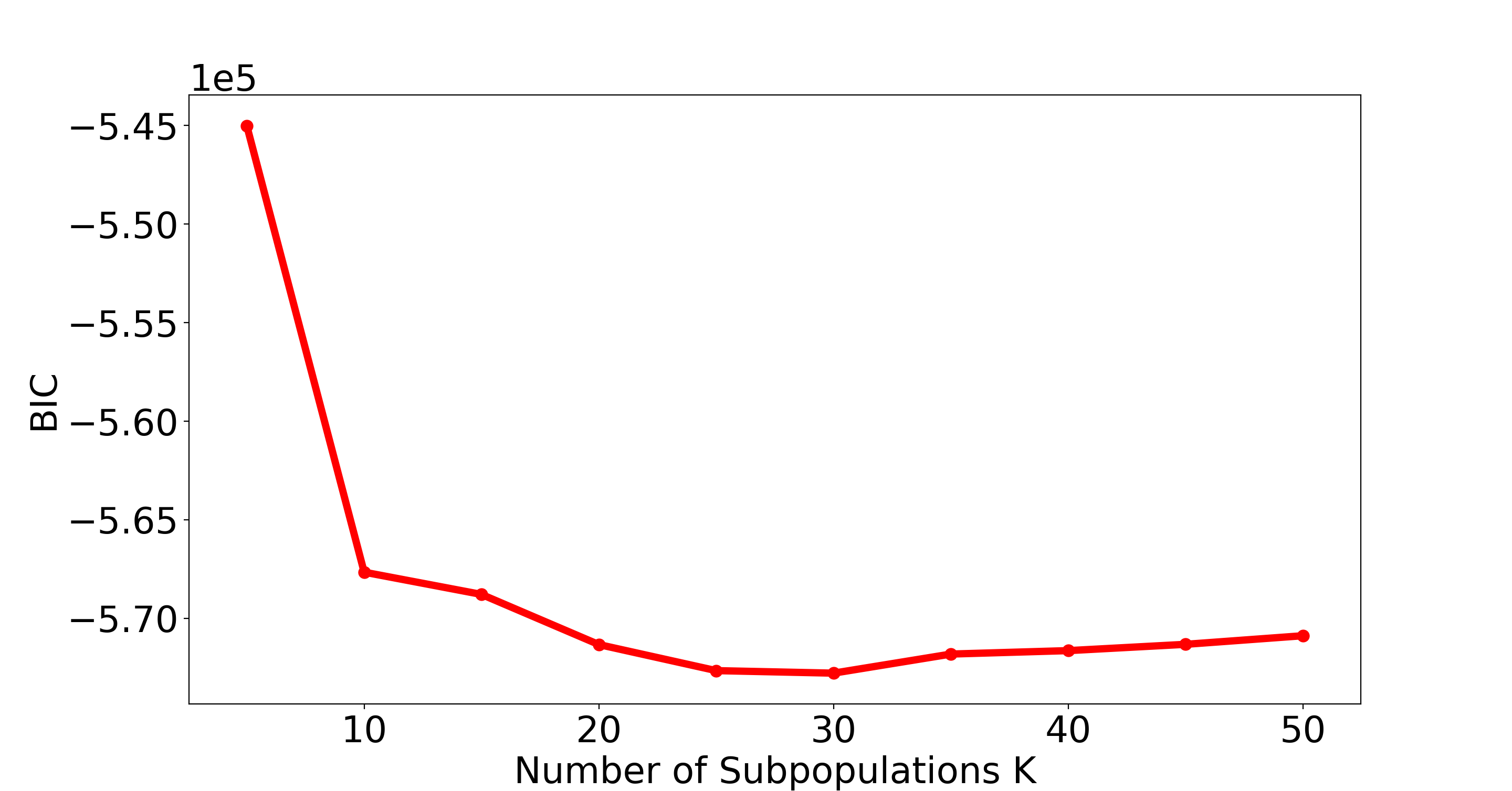
Figure 1: The Bayesian Information Criterion (BIC) computed over a grid of values of $K$ (blackin increments of 5) using the data of the SDSS DR8. The BIC is a model selection criterion based on the log-likelihood; the model with the lowest BIC blackvalue is preferred, blackindicating that in this case the optimal number of subpopulations is $K=25$.

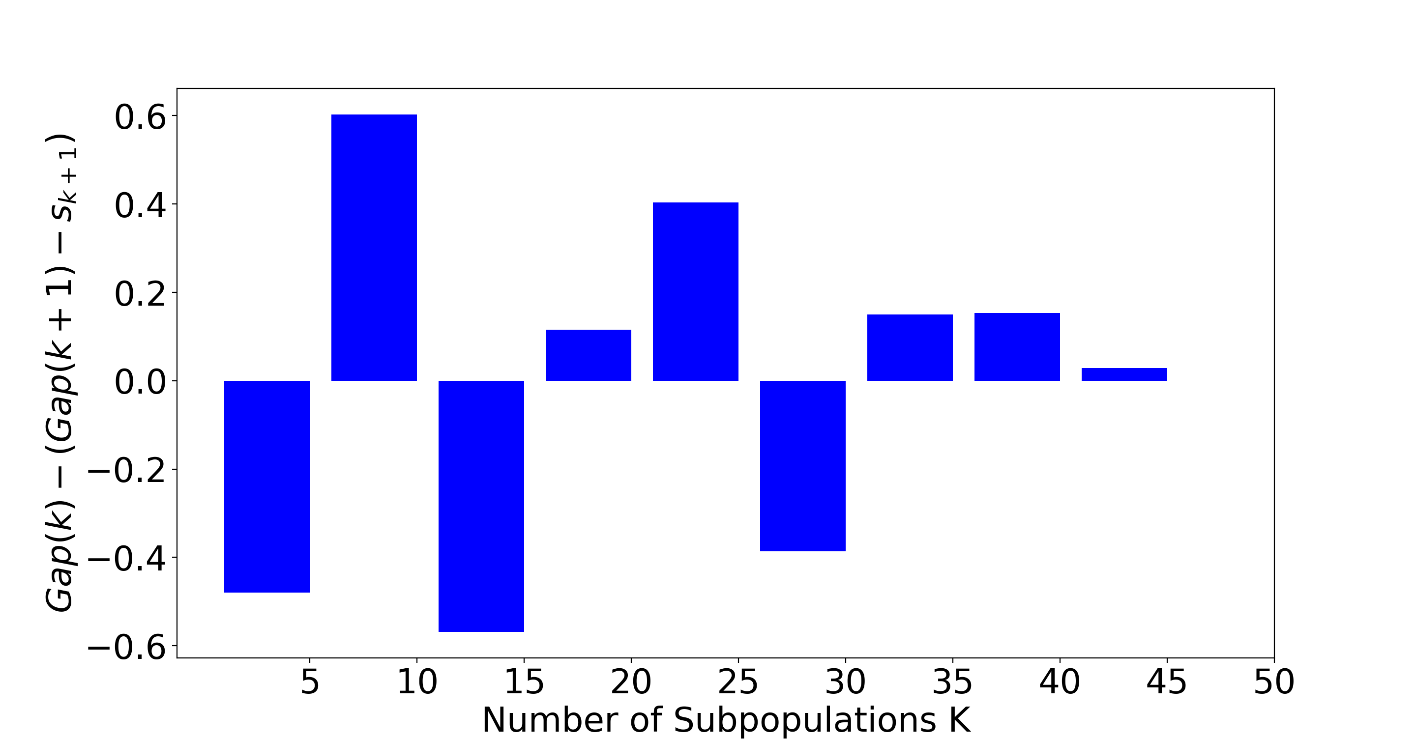
Figure 2: The Gap statistic computed over a grid of values of $K$ (blackin increments of 5) using the data of the SDSS DR8. The Gap statistic compares the intra-subpopulation distances between points in a given subpopulation with a null reference distribution of the data, blacki.e., a distribution with no obvious clustering. blackThis figure shows that the smallest value of $K$ for which the data measure exceeds the randomly generated measure is $K=10$.

Figure 3 displays the BPT diagnostic diagrams for blackSDSS DR8 with each point colour coded according to its most probable subpopulation among the $K=20$ fit. The means of the subpopulations are plotted for $k=1,\ldots,20$. blackTo visualize the spacial extent of each of the 20 subpopulation, Figure 4 plots the [N ii]$/$H$\alpha$ vs [O iii]$/$H$\beta$ diagnostic diagram for each subpopulation black(Subpopulation 18 contains very few objects, mostly capturing objects with large errors in the [O i]$/$H$\alpha$ ratios). We emphasize that the full 4-dimensional geometry of the subpopulations cannot be seen in the 2-dimensional projections.

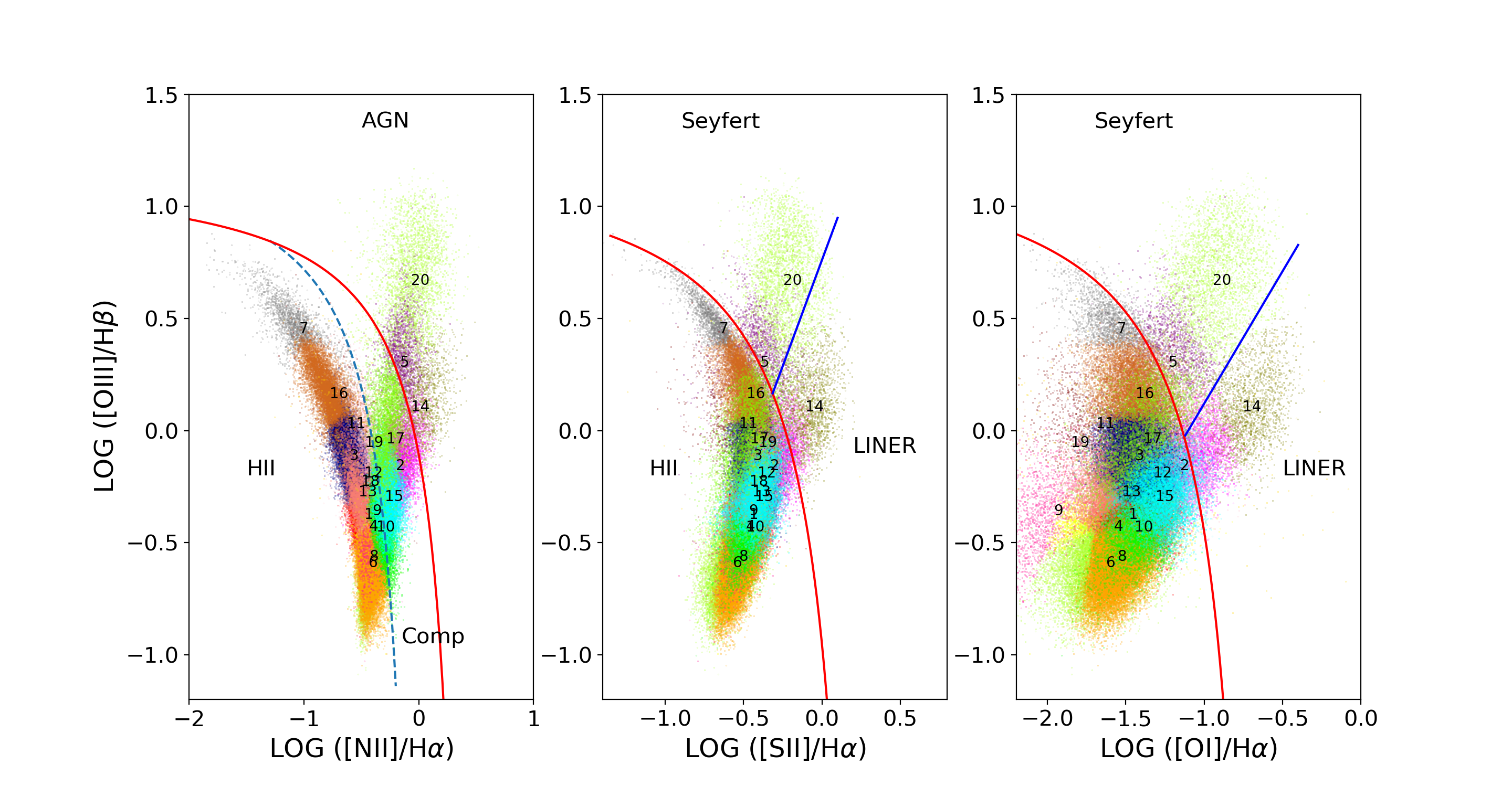
Figure 3: The BPT diagnostic diagrams for the blackSDSS DR8 sample; each galaxy is coloured according to its most probable allocation to one of the 20 subpopulations. The maximum ’starburst’ line of Kewley et al. (2001) is shown blackby the solid red line and the empirical upper bound on SFG of Kauffmann et al. (2003) is plotted as dashed blue line. The empirical line for distinguishing Seyferts and LINERs of Kewley et al. (2006) is depicted blackby the solid blue line.

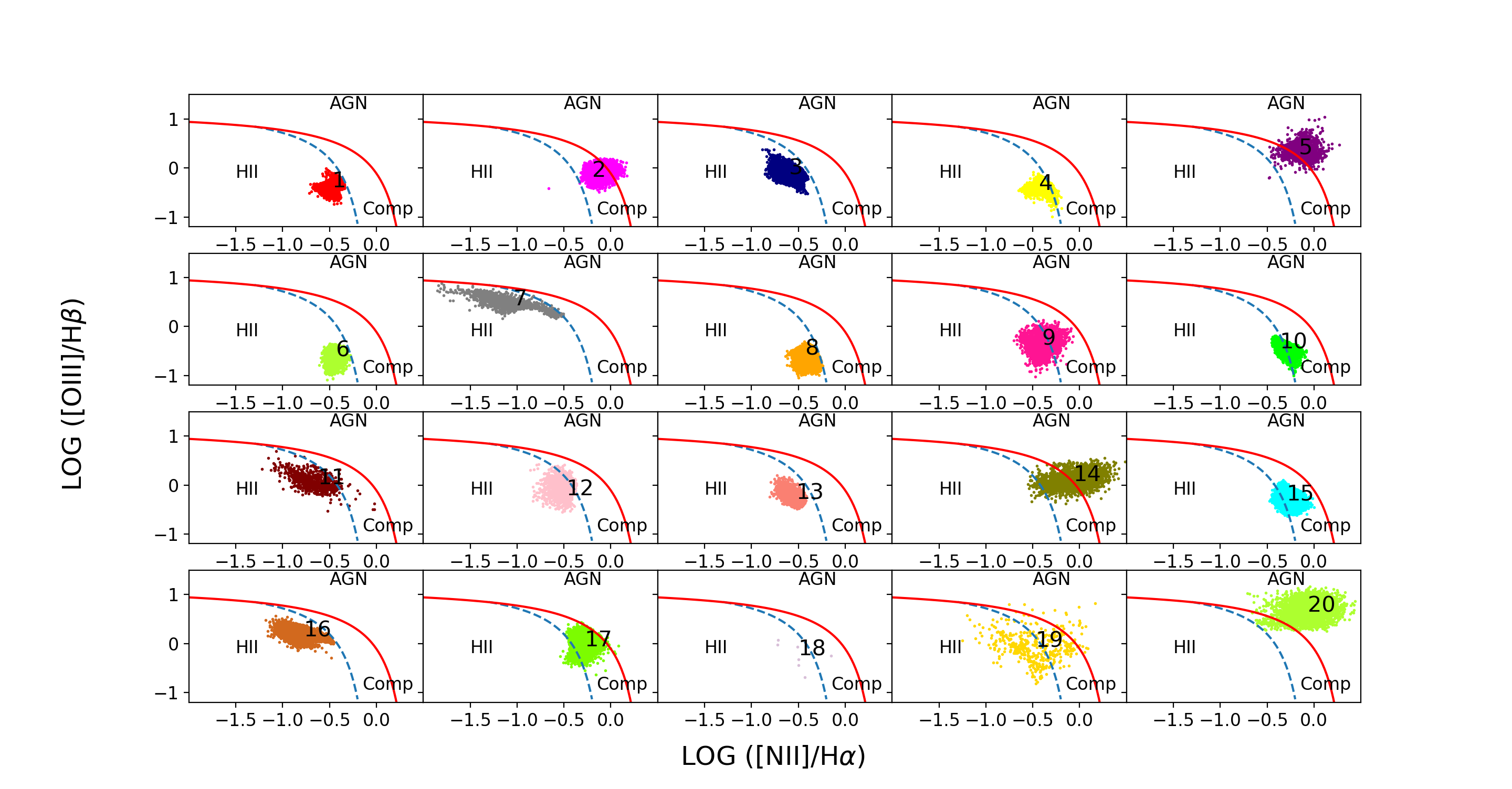
Figure 4: blackThe 20 subpopulations plotted on the [N ii]$/$H$\alpha$ vs [O iii]$/$H$\beta$ projection of the 4-dimensional diagnostic diagram. The subpopulations are numbered following the scheme in Figure 3. This figure shows the spatial extent of each subpopulation and their location with respect to the standard diagnostic lines in the [O iii]$/$H$\beta$ diagram. Since these are 2-dimensional projection of the 4-dimensional distribution in each subpopulation, they only give an indication of the extent and location of each subpopulation.

SoDDA associates each of the black20 subpopulations with one activity class based on blackthe projection of their mean on the 2-dimensional BPT diagnostic diagrams, and their location with respect to the activity-class separating lines reported in Kewley et al. (2006). The allocations are blackgiven in Table 1 for the 20 subpopulations means. blackAll but subpopulation 5 can be clearly associated with one activity class in all three diagnostic planes. The mean of subpopulation 5 is located within the Seyfert class, but its extent transcends the Composite and Seyfert classes. Since the main discriminator between Composite galaxies and Seyferts is the [N ii]$/$H$\alpha$ diagnostic and the mean of this subpopulation is clearly above the maximum ‘starburst’ line on the BPT diagrams introduced by Kewley et al. (2001) as an upper bound of SFGs, we include Subpopulation 5 in the Seyfert class. After combining the 20 subpopulations to form the 4 galaxy classes as described in Table 1, we compute the posterior probability of each galaxy being a SFG, Seyfert, LINER, or Composite using Equation 11. blackThe second row in Figure 5 shows the BPT diagnostic diagrams for SDSS blackDR8 with each galaxy colour coded according to its most probable galaxy class (red for SFGs, yellow for Seyferts, blue for LINERs, and green for the Composites) under SoDDA. blackTo highlight the spatial extent of each cluster, we plot the BPT diagrams for each activity class (SFGs, Seyferts, LINERs and Composites) individually in Figure 6.

Table 1: The suggested classification of the black20 subpopulations means.

Class	Subpopulation ID
SFG	black1, 3, 4, 6, 7, 8, 9, 10, 11, 12, 13, 16, 19
Seyferts	black5, 20
LINER	black14
Composites	black2, 15, 17, 18

Figure 7 depicts a 3-dimensional projection of the SDSS blackDR8 sample on the ([N ii]$/$H$\alpha$, [S ii]$/$H$\alpha$, [O iii]$/$H$\beta$) volume. This 3-dimensional projections illustrate the complex structure of the 4 galaxy activity classes. 3-dimensional rotating projections can be found at http://hea-www.harvard.edu/AstroStat/etc/gifs.pdf

blackThe data used for Figs 7, 5, 6 are presented in Table 2. This table gives the SoDDA-based probability that each galaxy in the sample considered here belongs to each one of the activity classes, along with the galaxy’s SPECOBJID, the key diagnostic line-ratios, and the activity classification based on the class with the highest probability. Table 2 contains the details for five galaxies of the sample we used. We include the table for the entire sample in the online version of the paper.

Table 2: blackActivity classification of the emission-line galaxies in the SDSS-DR8 based on the SoDDA. Column (1): SPECOBJID in SDSS DR8; Columns (2), (3), (4), (5): Logarithm of the diagnostic line-ratios (see SS3); Columns (6), (7), (8), (9): Probability that a galaxy belongs to each one of the 4 activity classes based on the SoDDA analysis; Column (10): Highest-ranking activity class: 0 for SFGs, 1 for Seyferts, 2 for LINERs, and 3 for Composites. We include the table for the entire sample in the online version of the paper.

	Line Ratio				SoDDA Probability
SPECOBJID	$\log$([N ii]$/$H$\alpha$)	$\log$([S ii]$/$H$\alpha$)	$\log$([O i]$/H\alpha$)	$\log$([O iii]$/$H$\beta$)	SFG	Seyfert	LINER	Composite	Activity Class
299491051364706304	-0.525441	-0.556073	-1.623533	-0.621178	0.992937	0.000052	3.217684e-09	0.007011	0
299492700632147968	-0.442478	-0.479489	-1.467312	-0.572390	0.983635	0.000046	8.869151e-08	0.016319	0
299493525265868800	-0.516100	-0.482621	-1.482500	-0.262816	0.989069	0.000207	7.396101e-07	0.010723	0
299493800143775744	-0.665688	-0.392920	-1.630935	-0.081032	0.999946	0.000007	1.841213e-09	0.000048	0
299494075021682688	-0.305985	-0.285281	-1.293723	-0.274226	0.189374	0.006725	7.278570e-04	0.803174	3

SoDDA provides a robust classification for the vast majority of the galaxies in the SDSS DR8 sample. For $87.8\%$ of the galaxies, $\max_{c}\rho_{ic}$ is greater than 75%. That is, the most probable class for each of $87.8\%$ of the galaxies has a posterior probability greater than 75%, indicating strong confidence in the adopted classification (the difference in the classification probability with the second largest class is at least 50%). black The difference between the largest and the second largest $\rho_{ic}$ (among the classes for each object), is a good indicator of the uncertainty of the classification. We find that this difference is greater than $50\%$ for $88.3\%$ of the galaxies, suggesting that the classifications are robust for the vast majority of the sample. The difference between the $\max_{c}\rho_{ic}$ and the second largest $\rho_{ic}$ is smaller than $10\%$ for $2.1\%$ of the galaxies, and smaller than $1\%$ for only $0.17\%$ of the galaxies. This indicates that the classification is uncertain for very few galaxies in the overall sample. This is illustrated in Figure 8 which plots $\max_{c}\rho_{ic}$, against the difference between $\max_{c}\rho_{ic}$ and the second largest $\rho_{ic}$ among the classes. The red lines denote a difference between the two highest values of $\rho_{ic}$ (among the classes) of $1\%$ and $50\%$.

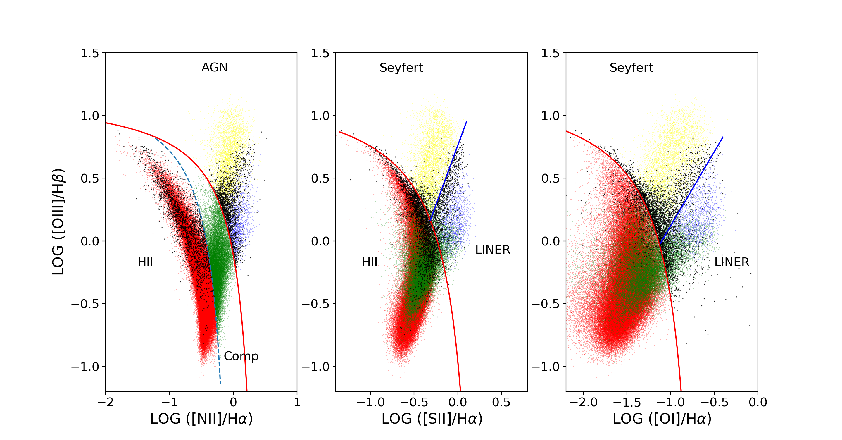
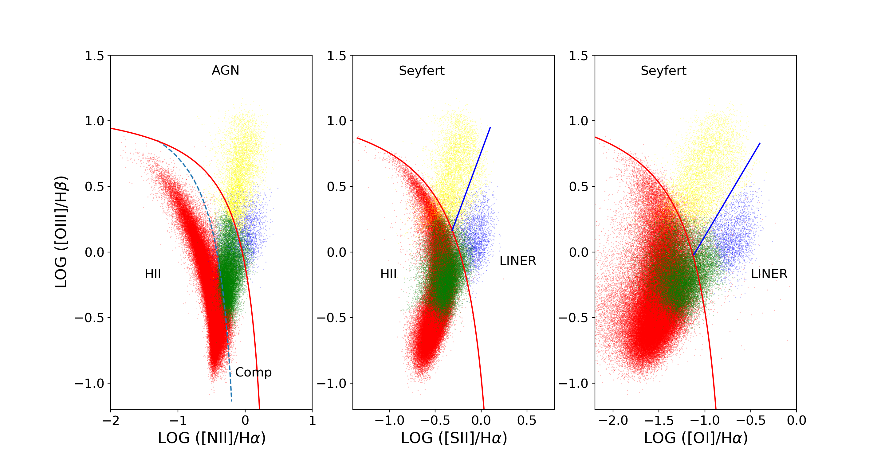
Figure 5: The BPT diagrams for the galaxies in the SDSS DR8 sample, based on the Kewley et al. (2006) scheme (top) and SoDDA (bottom). Each galaxy is colour coded according to its classification: red for SFGs, yellow for Seyferts, blue for LINERs, green for the Composite galaxies, and black for the Contradicting classifications. Note the lack of any contradicting classifications (black points) in the SoDDA results (bottom). For reference we also plot the the maximum ’starburst’ line of Kewley et al. (2001) (solid red), the empirical upper bound on SFG of Kauffmann et al. (2003) (dashed blue), and the empirical line distinguishing Seyferts and LINERs (Kewley et al. 2006; solid blue). 3-dimensional rotating projections of the 4-dimensional diagram of the SoDDA classification (depicted in the bottom row of the figure in 2-dimensional projections) are available online: http://hea-www.harvard.edu/AstroStat/etc/gifs.pdf. The animated figures can also be found as supplementary material.

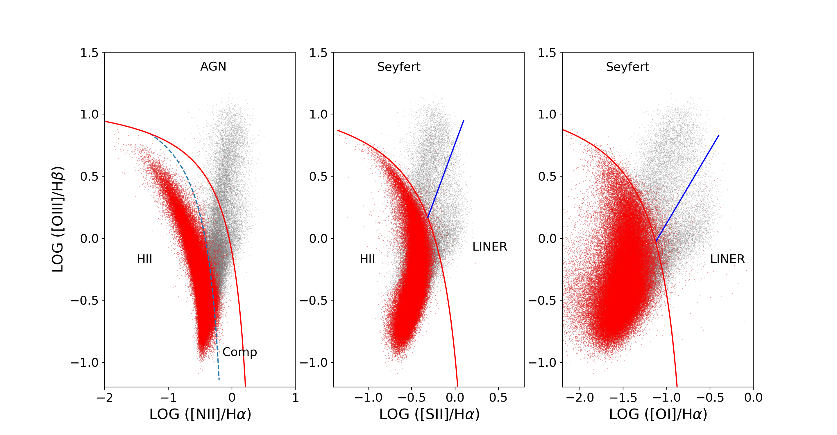
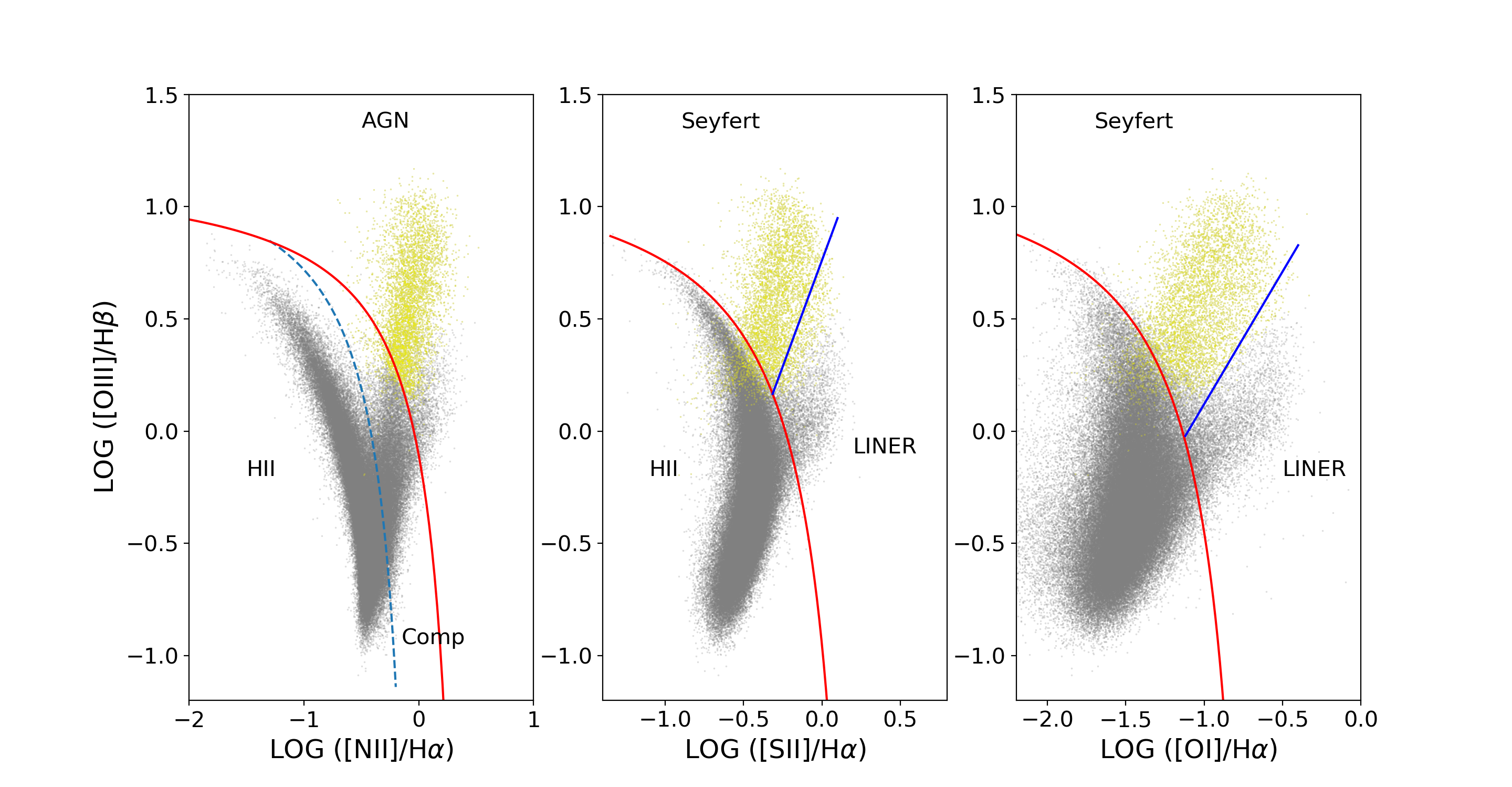
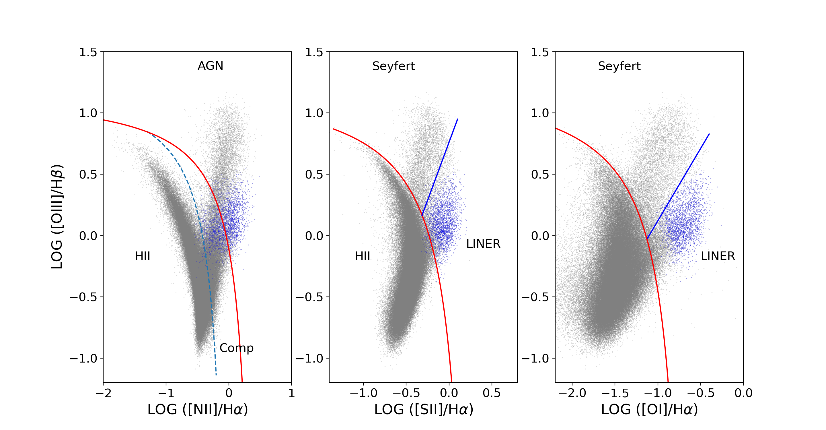
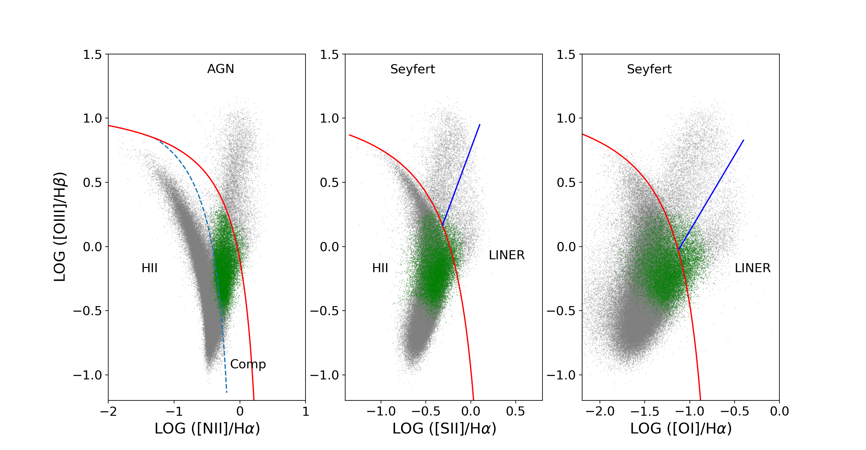
Figure 6: The locus of galaxies classified into the different activity types using SoDDA plotted on the three BPT diagrams. Each set of panels shows a different class (clockwise from top left): (a) SFGs (red), (b) Seyfert (yellow); (c) LINERs (blue), (d) Composite (green). For reference the full sample is also plotted in grey. The maximum ’starburst’ line of Kewley et al. (2001) is plotted as a solid red line, the empirical upper bound on SFG of Kauffmann et al. (2003) is plotted as a dashed blue line, and the empirical line distinguishing Seyferts and LINERs (Kewley et al., 2006) is plotted as a solid blue line.

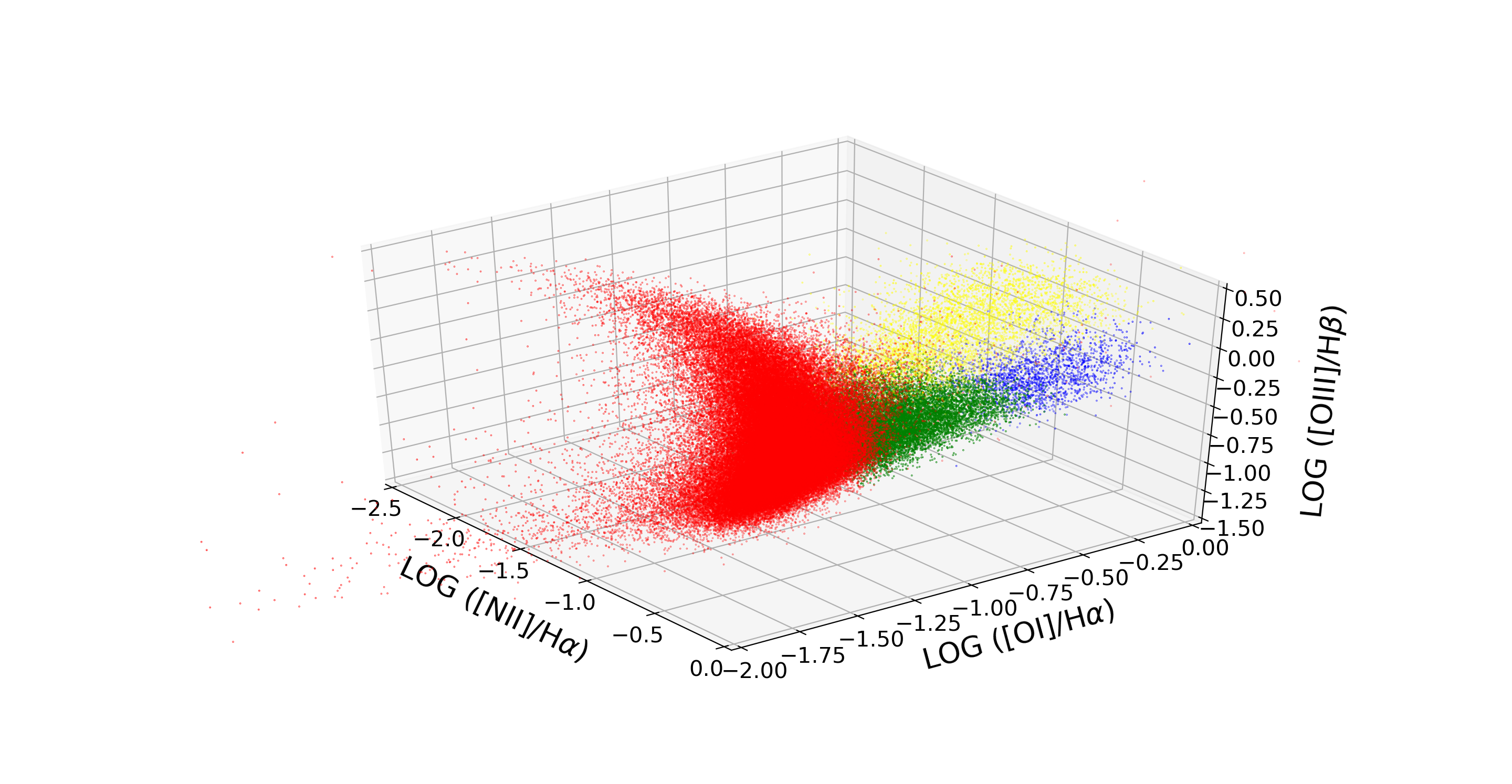
Figure 7: A 3-dimensional projection of the SDSS blackDR8 sample blackused in our study on the ([N ii]$/$H$\alpha$, [S ii]$/$H$\alpha$, [O iii]$/$H$\beta$) volume, in which each galaxy is colour coded according to its SoDDA classification (red for SFGs, yellow for Seyferts, blue for LINERs and green for the Composites). The 3-dimensional projections illustrates the complex structure of the 4 galaxy activity classes. Each of the four 3-dimensional rotating projection of the full 4-dimensional diagram are available online: http://hea-www.harvard.edu/AstroStat/etc/gifs.pdf.

blackIn order to assess the stability of the classification we randomly select a bootstrap sample consisting of 90% of the SDSS DR8 data (sampled without replacement). Using the bootstrap sample, we retune the classifier by estimating the means, weights, and covariance matrices for the black20 subpopulations, assigning each to one of the 4 activity classes, and recalculating the probability that each galaxy belongs to each of the 4 classes. We denote these probabilities, $\rho_{ic}^{\rm boot}$, to distinguish them from those computed with the full SDSS DR8 sample, namely $\rho_{ic}$. There is excellent agreement between the original classification and that obtained using the bootstrap sample. Specifically, black94.9% of the galaxies are classified into the same activity type with both classifiers. blackSimilarly, 88.4% of the galaxies classified as Composites (the class with the largest degree of mixing with the other classes; c.f. Figs. 5, 4) using the original classifier are classified in the same way using the set of parameters obtained from using the bootstrap sample. The figures are 95.1% for Seyferts, 98.9% for LINERs, and 95.8% for SFGs.

Overall there is little difference between the class probabilities of the individual galaxies computed with the full data and with the bootstrap sample. To illustrate this, we plot $\max_{c}\rho_{ic}-\max_{c}\rho_{ic}^{\rm boot}$ against $\max_{c}\rho_{ic}$ in Figure 9. Galaxies that are classified differently by the two classifiers are plotted in red. Again, there is excellent agreement: Not only is the classification of the vast majority of galaxies the same for both classifiers, but the probabilities of belonging to the chosen class are both similar and high. Of the galaxies (5.1%) that are classified differently, 89.9% have $\max_{c}\rho_{ic}<75\%$, meaning their classification was not clear to begin with. Overall, our classifier appears robust to the choice of sample used for defining the classification clusters.

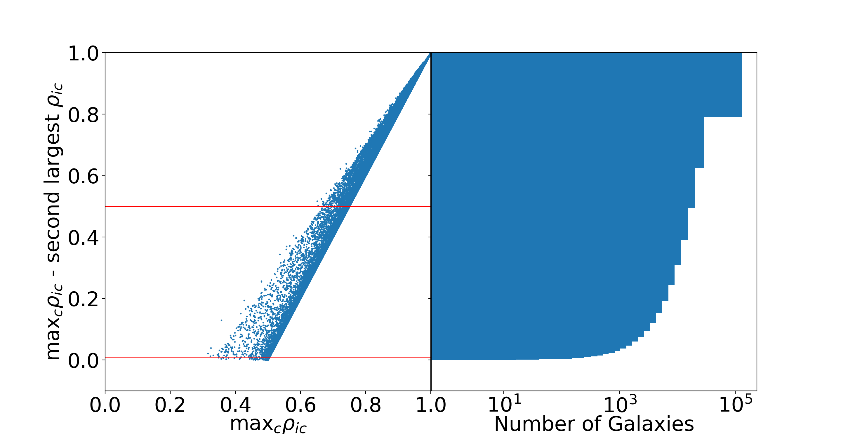
Figure 8: The difference between the SoDDA probabilities of the most likely and second most likely class for each galaxy in the SDSS D8 sample. The difference is plotted against the probability of the most likely class. The red lines corresponds to a difference of $1\%$ and $50\%$. Only 0.21% of the galaxies exhibit a difference between the probabilities of the most and second most likely classes of less than 1%. $87.8\%$ of the galaxies have $\max_{c}\rho_{ic}>75\%$, indicating a highly confident classification. The histogram in the right of the plot shows the cumulative distribution of the difference between the maximum and the second highest probability. It is clear that more than 75% of the galaxies have difference well above 0.8.

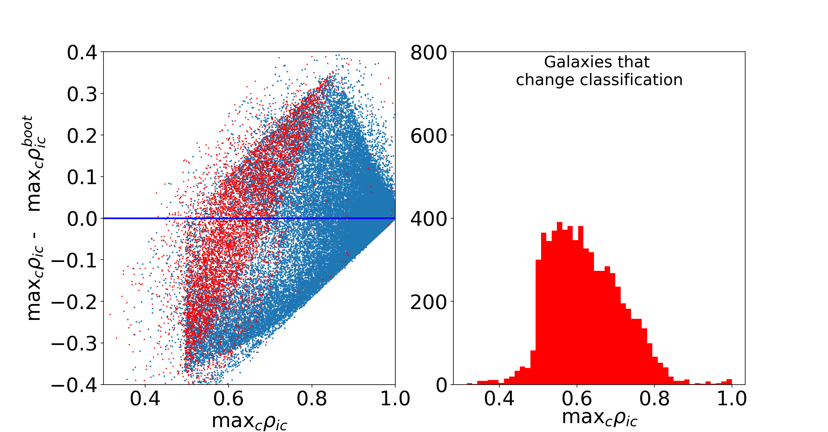
Figure 9: (left)A plot of the difference between the class probabilities of the individual galaxies computed with the full data and with the bootstrap sample, namely a plot of $\max_{c}\rho_{ic}-\max_{c}\rho_{ic}^{\rm boot}$ against $\max_{c}\rho_{ic}$. Galaxies that are classified differently by the two schemes are plotted in red. The vast majority of galaxies have the same classification under both schemes; those that do not (5.1% of the full sample) have $\max_{c}\rho_{ic}<75\%$ (89.9% of them), meaning their classification was not clear to begin with. (right) A histogram of the distribution of the maximum probability (i.e. the probability of the highest class $\max_{c}\rho_{ic}$) for the objects that change classification in the bootstrap analysis. blackThe vast majority of the objects have $\max_{c}\rho_{ic}<0.75$. Note the sheer difference in the number of objects that change classification with respect to the total number of objects.

4 Comparison with 2-dimensional Classification Scheme

In contrast to blackthe standard approach of using hard thresholds to define the different classes, SoDDA uses soft clustering. black This allows for the natural mixing between the different classes given that there is a continuous distribution of galaxies in the emission-line diagnostic diagrams. We thus calculate the posterior probability of each galaxy belonging to each activity class. Moreover, SoDDA is not based on any particular set of blacktwo-dimensional projections of the distributions of emission-line ratios, but rather it takes into account the joint distribution of all 4 emission-line ratios, blackwhich maximizes the discriminating power of the diagnostic. Thus, the main difference between the two schemes is that SoDDA does not produce blackcontradictory classifications for the same galaxy. Rather SoDDA provides a single coherent summary blackbased on all diagnostic line ratios: a posterior membership probability for each galaxy.black This allows us to select a sample of galaxies at the desired level of confidence, either in terms of absolute probability of belonging in a given class, or in terms of the odds in belonging in different classes.

Table 3: A 3-way classification table that compares the SoDDA classification with the standard, 2-dimensional classification scheme (Kewley et al., 2006). Each cell has 3 values: the number of galaxies with (i) $\rho_{ic}\geq 75\%$, (ii) $50\%\leq\rho_{ic}<75\%$, and (iii) $\rho_{ic}<50\%$, where $\rho_{ic}$ is the posterior probability that galaxy $i$ belongs to galaxy class $c$ under SoDDA. blackContradictory classifications are called ambiguous classifications by Kewley et al. (2006).

SoDDA	Kewley et al. (2006)
		SFGs				Seyferts				LINERs				Comp				Contradictory				Total
		$\geq 75\%$	$50\%-75\%$	$<50\%$		$\geq 75\%$	$50\%-75\%$	$<50\%$		$\geq 75\%$	$50\%-75\%$	$<50\%$		$\geq 75\%$	$50\%-75\%$	$<50\%$		$\geq 75\%$	$50\%-75\%$	$<50\%$		$\geq 75\%$	$50\%-75\%$	$<50\%$
	SFGs	98363	3521	42		4	2	0		0	1	0		1535	2369	113		1745	99	13		101647	5992	168
	Seyferts	0	1	1		3462	241	1		30	48	7		80	336	42		532	497	45		4104	1123	96
	LINERs	0	0	0		0	0	0		811	354	21		436	255	23		34	44	26		1281	653	70
	Comp	43	791	38		0	0	0		21	147	24		7545	6438	207		157	208	46		7766	7584	315

A 3-way classification table that compares SoDDA with the blackcommonly used scheme proposed by Kewley et al. (2006) appears in Table 3. Each cell has 3 values: the number of galaxies with (i) $\rho_{ic}\geq 75\%$, (ii) $50\%\leq\rho_{ic}<75\%$, and (iii) $\rho_{ic}<50\%$, where $\rho_{ic}$ is the posterior probability that galaxy $i$ belongs to galaxy class $c$. For example, the cell in the first row and first column shows that of the galaxies that both the SoDDA and the Kewley et al. (2006) method classify as SFG, black98,363 are SFGs under SoDDA with probability greater than $75\%$, black3,521 with probability between $50\%$ and $75\%$, and only black42 with probability less than $50\%$. blackIn general there is very good agreement between the SoDDA and the Kewley et al. (2006) classification for the star-forming and the Seyfert galaxy classes. In the case of LINERs there is also reasonable agreement, but with a larger fraction of galaxies classified in the intermediate confidence ($50\%\leq\rho_{ic}<75\%$) regime. In the case of composite objects, however, the fraction of galaxies classified in the intermediate or low ($\rho_{ic}<50\%$) confidence regime increases dramatically. This is a result of the overlap between the composite and the other activity classes in the $\log($[N ii]$/$H$\alpha$), $\log$([S ii]$/$H$\alpha$), and $\log$([O iii]$/$H$\beta$), but not for ([O i]$/H\alpha$ - [O iii]$/H\beta$) and the ([S ii]/H$\alpha$)- [O iii]$/H\beta$) diagnostics (Fig. 5, 6). blackThe majority of the galaxies that have contradictory classifications according to Kewley et al. (2006) are estimated with the SoDDA to be SFGs, and increasingly reduced fractions are allocated to the Seyfert, LINER, and Composite classes.

black In Figure 5 we show the classification based on the diagnostic lines presented in Kewley et al. (2006) (top panels) along with the classification based on the SoDDA method. The colour coding of the different classes is the same in both panels (red for SFGs, yellow for Seyfert, blue for LINERs, green for composite galaxies). Objects with contradictory classifications in the top panel are marked in black. blackThe overlap between the composite galaxies (green) and the SFGs (red) is clear in the SoDDA classification (middle and right panels of Figure 5), indicating that the 2-dimensional projection of this 4-dimensional parameter space is insufficient for capturing its complex structure and accurately classifying the galactic activity. blackThe use of hard boundaries defined independently in the 2-dimensional projections is responsible for those galaxies with contradictory classification. On the other hand the probabilistic approach of SoDDA simultaneously accounts for the 4-dimensional structure of the data space and inherently alleviates these inconsistent classifications, while at the same time giving a confident classification of the galaxies to activity classes.

5 Multidimensional Decision Boundaries

blackIn order to provide a more immediately usable diagnostic in the spirit of the classification lines of Kauffmann et al. (2003) and Kewley et al. (2006), which however, simultaneously employ the information in all diagnostic lines, we use a support vector machine (SVM) (Cortes & Vapnik, 1995) to obtain multidimensional decision boundaries based on the SoDDA results. A SVM is a discriminative classifier formally defined by a separating hyperplane. In other words, given classified galaxies, the algorithm outputs an optimal hyperplane which can be used to categorize new unlabelled galaxies. blackThis hybrid approach uses the SoDDA classification to disentangle the complex multi-dimensional structure of the overlapping clusters, while providing easy to use diagnostic surfaces in the spirit of the commonly BPT-like diagnostics.

5.1 4-dimensional Decision Boundaries

The input data blackfor the derivation of the multidimensional decision boundaries are the 4 emission line ratios for the galaxies in the blackSDSS DR8 sample (i.e. $x$), and the classification for each galaxy blackas obtained with SoDDA black(i.e., $y$). We use the scikit-learn Python library to fit the SVM model, employing a linear kernel function. blackA more complex function did not provide an improvement significant enough to justify its use, black especially given the simplicity of a linear kernel. The SVM algorithm requires tuning the cost factor parameter $C$, that sets the width of the margin between hyperplanes separating different classes of objects. After a grid search in a range of values for $C$, we blackadopt a value of $C=1$ based on 10-fold cross-validation. $\cal K$-fold cross-validation is a model validation method for estimating the performance of the model. The data is split in $\cal K$ roughly equal parts. For each $\kappa\in(1,...,\cal K)$ we fit the model in the other $\cal{K}$$-1$ parts of the data and calculate the prediction error of the fitted model when predicting the $\kappa$th part of the data (the error is effectively the number of inconsistent classifications between the SVM analysis on the the $\kappa$th part of the data and the classifications obtained by SoDDA for the same galaxies). By repeating this procedure for a range of values for the model parameters ($C$), we choose the values of $C$ that give us the SVM model with the minimum expected prediction error.

Using the SoDDA classification, we employ an SVM approach to define multidimensional surfaces separating the galaxy activity classes. More specifically, we find an optimal separation hyperplane using the 4 emission line ratios for the galaxies from blackthe SDSS DR8 sample and their most probable classification obtained by SoDDA as inputs. The 4-dimensional linear decision boundaries for the four galaxy classes are defined below.

SFG:

$$-7.31\log([\text{\text{N\,{ii}}}]/\text{H}\alpha) +2.75\log([\text{\text{S\,{ii}}}]/\text{H}\alpha)-1.41\log(\text{[\text{O\,{i}}]}/\text{H}\alpha)$$

$$-5.91\log(\text{[\text{O\,{iii}}]}/\text{H}\beta)>1.92$$ (12)

$$-5.32\log([\text{\text{N\,{ii}}}]/\text{H}\alpha) -6.37\log([\text{\text{S\,{ii}}}]/\text{H}\alpha)-3.40\log(\text{[\text{O\,{i}}]}/\text{H}\alpha)$$

$$-0.42\log(\text{[\text{O\,{iii}}]}/\text{H}\beta)>6.51$$ (13)

$$-23.01\log([\text{\text{N\,{ii}}}]/\text{H}\alpha) +0.93\log([\text{\text{S\,{ii}}}]/\text{H}\alpha)-5.30\log(\text{[\text{O\,{i}}]}/\text{H}\alpha)$$

$$-8.10\log(\text{[\text{O\,{iii}}]}/\text{H}\beta)>16.38$$ (14)

Seyferts:

$$-7.31\log([\text{\text{N\,{ii}}}]/\text{H}\alpha) +2.75\log([\text{\text{S\,{ii}}}]/\text{H}\alpha)-1.41\log(\text{[\text{O\,{i}}]}/\text{H}\alpha)$$

$$-5.91\log(\text{[\text{O\,{iii}}]}/\text{H}\beta)<1.92$$ (15)

$$0.37\log([\text{\text{N\,{ii}}}]/\text{H}\alpha) -4.55\log([\text{\text{S\,{ii}}}]/\text{H}\alpha)-7.21\log(\text{[\text{O\,{i}}]}/\text{H}\alpha))$$

$$+11.65\log(\text{[\text{O\,{iii}}]}/\text{H}\beta)>10.02$$ (16)

$$7.14\log([\text{\text{N\,{ii}}}]/\text{H}\alpha) -3.12\log([\text{\text{S\,{ii}}}]/\text{H}\alpha)+0.46\log(\text{[\text{O\,{i}}]}/\text{H}\alpha)$$

$$+16.08\log(\text{[\text{O\,{iii}}]}/\text{H}\beta)>2.82$$ (17)

LINERs:

$$-5.32\log([\text{\text{N\,{ii}}}]/\text{H}\alpha) -6.37\log([\text{\text{S\,{ii}}}]/\text{H}\alpha)-3.40\log(\text{[\text{O\,{i}}]}/\text{H}\alpha)$$

$$-0.42\log(\text{[\text{O\,{iii}}]}/\text{H}\beta)<6.51$$ (18)

$$0.37\log([\text{\text{N\,{ii}}}]/\text{H}\alpha) -4.55\log([\text{\text{S\,{ii}}}]/\text{H}\alpha)-7.21\log(\text{[\text{O\,{i}}]}/\text{H}\alpha)$$

$$+11.65\log(\text{[\text{O\,{iii}}]}/\text{H}\beta)<10.02$$ (19)

$$-1.04\log([\text{\text{N\,{ii}}}]/\text{H}\alpha) +8.94\log([\text{\text{S\,{ii}}}]/\text{H}\alpha)+6.48\log(\text{[\text{O\,{i}}]}/\text{H}\alpha)$$

$$+6.69\log(\text{[\text{O\,{iii}}]}/\text{H}\beta)>-6.90$$ (20)

Composites:

$$-23.01\log([\text{\text{N\,{ii}}}]/\text{H}\alpha) +0.93\log([\text{\text{S\,{ii}}}]/\text{H}\alpha)-5.30\log(\text{[\text{O\,{i}}]}/\text{H}\alpha)$$

$$-8.10\log(\text{[\text{O\,{iii}}]}/\text{H}\beta)<16.38$$ (21)

$$7.14\log([\text{\text{N\,{ii}}}]/\text{H}\alpha) -3.12\log([\text{\text{S\,{ii}}}]/\text{H}\alpha)+0.46\log(\text{[\text{O\,{i}}]}/\text{H}\alpha)$$

$$+16.08\log(\text{[\text{O\,{iii}}]}/\text{H}\beta)<2.82$$ (22)

$$-1.04\log([\text{\text{N\,{ii}}}]/\text{H}\alpha) +8.94\log([\text{\text{S\,{ii}}}]/\text{H}\alpha)+6.48\log(\text{[\text{O\,{i}}]}/\text{H}\alpha)$$

$$+4.69\log(\text{[\text{O\,{iii}}]}/\text{H}\beta)<-6.90$$ (23)

Table 4 compares the SoDDA classification with the proposed classification from the SVM, while Table 5 compares the scheme from Kewley et al. (2006) with the SVM. We see excellent agreement between the SoDDA and the SVM-based classification. blackMore specifically, 99.0% of the galaxies classified as SFGs by SoDDA are classified in the same way as the SVM-based classification. The figures are 96.9% for Seyferts, 91.2% for LINERs, and 90.2% for Composites. blackSimilarly, we find very good agreement between the traditional 2-dimensional diagnostics of (Kewley et al., 2006) and the SVM method in the cases of SFGs and Seyfert galaxies (Table 5). For Composite objects and LINERs we find a larger number of objects for which we obtain a different classification based on the two methods. The largest discrepancy is in the case of LINERs (agreement for 80% of the LINER sample), which we attribute to the complex shape on the distribution of the Composite objects for which the SoDDA analysis shows that they extend to the locus of LINERs (Figs. 5, 6). We note that such discrepancies are expected, given the ad-hoc definition of the activity classes, particularly in the case of composite galaxies.

Table 4: blackComparison of the SoDDA classification with that of the 4-dimensional SVM ([O iii]$/$H$\beta$, [N ii]$/$H$\alpha$, [S ii]$/$H$\alpha$ and [O i]$/$H$\alpha$ space).

SVM	SoDDA
		SFGs	Seyferts	LINERs	Composites	Total
	SFGs	106782	14	13	1330	108139
	Seyferts	36	5157	39	115	5347
	LINERs	22	9	1828	85	1944
	Composites	967	143	124	14135	15369
	Total	107807	5323	2004	15665

Table 5: blackComparison of the classifications of a 4-dimensional SVM with that of the method by Kewley et al. (2006) ([O iii]$/$H$\beta$, [N ii]$/$H$\alpha$, [S ii]$/$H$\alpha$ and [O i]$/$H$\alpha$ space). blackContradictory classifications are called ambiguous classifications by Kewley et al. (2006).

SVM	Kewley et al. (2006)
		SFGs	Seyferts	LINERs	Composites	Contradictory	Total
	SFGs	102455	0	0	3987	1697	108139
	Seyferts	0	3708	107	478	1054	5347
	LINERs	0	0	1176	677	91	1944
	Composites	345	2	181	14237	604	15369
	Total	102800	3710	1464	19379	3446

5.2 3-dimensional Decision Boundaries

Because the [O i] line is generally blackvery weak and hence hard to blackmeasure, it is common to blackuse the flux ratios of the five other strong lines in the optical spectrum: $\log($[N ii]$/$H$\alpha$), $\log$([S ii]$/$H$\alpha$), and $\log$([O iii]$/$H$\beta$). Thus, we black use the SoDDA classification (Section 3) as the basis for the definition of decision boundaries by applying the SVM algorithm in the 3-dimensional space defined by the ($\log($[N ii]$/$H$\alpha$), $\log$([S ii]$/$H$\alpha$), and $\log$([O iii]$/$H$\beta$) emission-line ratios. The resulting 3-dimensional decision surfaces for the four galaxy classes are presented below.

SFG:

$$-7.27\log([\text{\text{N\,{ii}}}]/\text{H}\alpha) +1.523\log([\text{\text{S\,{ii}}}]/\text{H}\alpha)$$

$$-7.02\log(\text{[\text{O\,{iii}}]}/\text{H}\beta)>0.25$$ (24)

$$-4.08\log([\text{\text{N\,{ii}}}]/\text{H}\alpha) -9.33\log([\text{\text{S\,{ii}}}]/\text{H}\alpha)$$

$$-1.93\log(\text{[\text{O\,{iii}}]}/\text{H}\beta)>3.28$$ (25)

$$-19.55\log([\text{\text{N\,{ii}}}]/\text{H}\alpha) -3.07\log([\text{\text{S\,{ii}}}]/\text{H}\alpha)$$

$$-7.10\log(\text{[\text{O\,{iii}}]}/\text{H}\beta)>9.45$$ (26)

Seyferts:

$$-7.27\log([\text{\text{N\,{ii}}}]/\text{H}\alpha) +1.523\log([\text{\text{S\,{ii}}}]/\text{H}\alpha)$$

$$-7.02\log(\text{[\text{O\,{iii}}]}/\text{H}\beta)<0.25$$ (27)

$$0.23\log([\text{\text{N\,{ii}}}]/\text{H}\alpha) -9.66\log([\text{\text{S\,{ii}}}]/\text{H}\alpha)$$

$$+9.29\log(\text{[\text{O\,{iii}}]}/\text{H}\beta)>4.03$$ (28)

$$7.22\log([\text{\text{N\,{ii}}}]/\text{H}\alpha) -2.77\log([\text{\text{S\,{ii}}}]/\text{H}\alpha)$$

$$+16.04\log(\text{[\text{O\,{iii}}]}/\text{H}\beta)>3.23$$ (29)

LINERs:

$$-4.08\log([\text{\text{N\,{ii}}}]/\text{H}\alpha) -9.33\log([\text{\text{S\,{ii}}}]/\text{H}\alpha)$$

$$-1.92\log(\text{[\text{O\,{iii}}]}/\text{H}\beta)<3.28$$ (30)

$$0.23\log([\text{\text{N\,{ii}}}]/\text{H}\alpha) -9.66\log([\text{\text{S\,{ii}}}]/\text{H}\alpha)$$

$$+9.29\log(\text{[\text{O\,{iii}}]}/\text{H}\beta)<4.03$$ (31)

$$-0.13\log([\text{\text{N\,{ii}}}]/\text{H}\alpha) +13.16\log([\text{\text{S\,{ii}}}]/\text{H}\alpha)$$

$$+5.04\log(\text{[\text{O\,{iii}}]}/\text{H}\beta)>-1.84$$ (32)

Composites:

$$-19.55\log([\text{\text{N\,{ii}}}]/\text{H}\alpha) -3.07\log([\text{\text{S\,{ii}}}]/\text{H}\alpha)$$

$$-7.10\log(\text{[\text{O\,{iii}}]}/\text{H}\beta)<9.45$$ (33)

$$7.22\log([\text{\text{N\,{ii}}}]/\text{H}\alpha) -2.77\log([\text{\text{S\,{ii}}}]/\text{H}\alpha)$$

$$+16.04\log(\text{[\text{O\,{iii}}]}/\text{H}\beta)<3.23$$ (34)

$$-0.13\log([\text{\text{N\,{ii}}}]/\text{H}\alpha) +13.16\log([\text{\text{S\,{ii}}}]/\text{H}\alpha)$$

$$+5.04\log(\text{[\text{O\,{iii}}]}/\text{H}\beta)<-1.84$$ (35)

The multidimensional decision boundaries achieve a mean classification accuracy of about $96.7\%$ based on 10-fold cross validation blackwith respect to the SoDDA classification. Table 6 compares the SoDDA classification with the proposed classification from the SVM, while Table 7 compares the scheme from Kewley et al. (2006) with the SVM. As with the 4-dimensional SVM classification, we have excellent agreement with the SoDDA classification and slightly worse agreement with the traditional 2-dimensional diagnostics. Surprisingly, we also find very blackgood agreement between the 3-dimensional and the 4-dimensional SVM diagnostics indicating that removing the fourth line ratio ([O i]$/$H$\alpha$) does not significantly affect the quality of the classification. blackMore specifically, 98.7% of the galaxies classified as SFGs by SoDDA are classified in the same way by the 3-dimensional SVM-based classification. The figures are 96.1% for Seyferts, 76.0% for LINERs, and 85.4% for Composites. In other words, removing the ([O i]$/$H$\alpha$) line ratio has no impact on the classification error for SFGs and the Seyferts, and blackresults in a different classification of $10.9\%$ of galaxies classified as LINERs by SoDDA and $3.7\%$ of galaxies classified as Composites by SoDDA, when compared to the complete 4-dimensional diagnostic.

Table 6: blackComparison of the classifications of SoDDA with that of the 3-dimensional SVM ([O iii]$/$H$\beta$, [N ii]$/$H$\alpha$, and [S ii]$/$H$\alpha$ space.

SVM	SoDDA
		SFGs	Seyferts	LINERs	Composites	Total
	SFGs	106416	16	27	1965	108424
	Seyferts	40	5117	111	108	5376
	LINERs	31	68	1524	217	1840
	Composites	1320	122	342	13375	15159
	Total	107807	5323	2004	15665

Table 7: blackComparison of the classifications of the 3-dimensional SVM and that of the method by Kewley et al. (2006) ([O iii]$/$H$\beta$, [N ii]$/$H$\alpha$, [S ii]$/$H$\alpha$ and [O i]$/$H$\alpha$ space). blackContradictory classifications are called ambiguous classifications by Kewley et al. (2006).

SVM	Kewley et al. (2006)
		SFGs	Seyferts	LINERs	Composites	Contradictory	Total
	SFGs	102750	0	0	3777	1897	108424
	Seyferts	0	3708	173	490	1005	5376
	LINERs	0	0	1101	601	138	1840
	Composites	50	2	190	14511	406	15159
	Total	102800	3710	1464	19379	3446

6 Discussion

We propose a new soft clustering scheme, the Soft Data-Driven Allocation (SoDDA) method, for classifying galaxies using emission-line ratios. Our method uses blackan optimal number of MG subpopulations in order to capture the multi-dimensional structure of the dataset and afterwards concatenate the MG subpopulations into clusters by assigning them to different activity types, based on the location of their means with respect to the loci of the activity classes as defined by Kewley et al. (2006).

The main advantages of this method areblack: (a) the use of all four optical-line ratios simultaneously, thus maximising the available informationblack, avoiding contradicting classifications, and black (b) treating each class as a distribution resulting in soft classification boundaries. blackThis allows us to account for the inherent overlap between the different activity classes stemming from the simultaneous presence of different excitation mechanisms with a varying degree of intensity. We achieve this by calculating the probability for an object to be associated with each one of these activity classes given their distribution in the multi-dimensional diagnostic space.

An issue with data-driven classification blackmethods is the question of whether the data have sufficient discriminating power to distinguish the different activity classes. A strong indication in this direction comes from the fact that the original BPT diagnostic (Baldwin et al., 1981) and its more recent redefinition by Kauffmann et al. (2003) and Kewley et al. (2006) was driven by the clustering of the activity classes in different loci on the 2-dimensional line-ratio diagrams. Furthermore, this distinction was supported by photoionisation models (Kewley et al., 2001, 2013) which indicate that while there is a continuous evolution of the location of sources on the 2-dimensional diagnostic diagrams as a function of their metallicity and hardness of the ionising continuum, star-forming galaxies occupy a distinct region of this diagram. In our analysis we follow a hybrid approach in which we identify clusters based on the multi-dimensional distribution of the object line-ratios, and we associate the clusters with activity types based on their location in the standard 2-dimensional diagnostic diagrams. This gives a physical blackinterpretation to each cluster, while tracing the multi-dimensional distribution of blacktheir line ratios.

The approach followed in this paper treats the multi-dimensional emission-line diagnostic diagram as a mixture of different classes. This is a more realistic approach as it does not assume fixed boundaries between the activity classes. Instead, it takes into account blackthe fact that the emission-line ratios of the different activity classes may overlap, blackwhich is reflected on the probabilities for an object to belong to a given class. This in fact is reflected in the often inconsistent classification between different 2-dimensional diagnostics (Ho et al., 1997; Yuan et al., 2010), and is clearly seen in the complex structure of the locus of the activity classes in blackthe 3-dimensional rotating diagnostics available blackin the online supplements. Therefore, the optimal way to characterize a galaxy is by calculating blackthe probability that it blackbelongs to each of the activity classes, black instead of associating it unequivocally with a given class. blackThis also gives us the possibility to define samples of different types of galaxies at various confidence levels.

Another advantage of this approach is that we take into account blackall available information for the activity classification of galactic nuclei. This is important given the complex shape of the multi-dimensional distributions of the emission line ratios (e.g. online 3-dimensional rotating diagnostics; see also Vogt et al. 2014). This way we increase the power of the 2-dimensional diagnostic tools, and eliminate the contradicting classifications they often give. This is demonstrated by the excellent agreement between the classification of the 4-dimensional diagnostic ([O iii]/H$\beta$, [O i]/H$\alpha$, [N ii]/H$\alpha$, [S ii]/H$\alpha$) with the 3-dimensional diagnostic excluding the often weak and hard to detect [O i] line ([O iii]/H$\beta$, [O i]/H$\alpha$, [N ii]/H$\alpha$, [S ii]/H$\alpha$; see 5.2). This agreement indicates that the loss of the diagnostic power of the [O i]/H$\alpha$ line (which blackis considered the main discriminator between LINERs and other activity classes (e.g. Kewley et al., 2006)) in the 4-dimensional diagnostic, can be compensated by the structure of the locus of the different activity classes which allows their distinction even in the 3-dimensional diagnostic.

blackA very similar approach was followed by de Souza et al. (2017) who modeled the ([O iii]/H$\beta$, [N ii]/H$\alpha$, EW(H$\alpha$)) 3-dimensional space with a set of 4 multi-dimensional Gaussians. The different number of Gaussian components required in our work is the result of the more complex structure of the distribution of the line ratios in the 4-dimensional ([O iii]/H$\beta$, [O i]/H$\alpha$, [N ii]/H$\alpha$, [S ii]/H$\alpha$) space, in comparison to the simpler shape in the 3-dimensional space explored by de Souza et al. (2017). The use of the EW(H$\alpha$) in the latter study instead of the [O i]/H$\alpha$ and [S ii]/H$\alpha$ line ratios allow the separation of star-forming from non star-forming galaxies (retired or passive; Cid Fernandes et al. (2011), Stasińska et al. (2015)).

Although the probabilistic clustering contains more information about the classification of each blackemission-line galaxy, the use of hard decision boundaries for classification is effective and closer to the standard approach used in the literature. Therefore, we also present hard classification criteria by employing SVM on the distribution of line-ratios of objects assigned to each activity class. The classification accuracy with these hard criteria is $\sim 98\%$ when compared to the soft classification (SoDDA). This indicates that the extended tails of the line-ratio distributions of the different activity classes result in only a small degree of overlap and hence misclassification compared to the results we get from SoDDA.

black Several efforts in the past have introduced activity diagnostic tools that combine information from multiple spectral bands and often including spectral-line ratios. For example Stern et al. (2005) and Donley et al. (2012) introduced the use of near and far-IR colours for separating star-forming galaxies from AGN. Dale et al. 2006 and Tommasin et al. 2010 have further developed the use of IR line diagnostics (involving for example emission lines from PAHs, [O iv], [Ne ii], [Ne iii]), initially proposed by Spinoglio & Malkan 1992. Such diagnostics have been used extensively in IR surveys in order to address the nature of heavily obscured galaxies, and they are going to be particularly useful for classifying objects detected in surveys performed with the James-Webb Space Telescope. black Composite diagnostic diagrams involving the [O iii]/H$\beta$ line-ratio and photometric data that are stellar-mass proxies Weiner et al. (2007), the stellar mass directly Juneau et al. (2011); Juneau et al. (2014), or photometric colours Yan et al. (2011), have been developed to classify high-redshift or heavily obscured objects. In a similar vein, Stasińska et al. (2006) propose a diagnostic based on the stellar-population age sensitive $\mathrm{4000\AA}$-break index compared with the equivalent width of the [O ii]$\mathrm{3727\AA}$ or the [N iii]$\mathrm{3869\AA}$ lines.

black These studies demonstrate that inclusion of information from photometric data, or wavebands other than optical, can extend the use of the diagnostic diagrams to higher redshifts, or increase the sensitivity of the standard diagrams in cases of heavily obscured galaxies or galaxies dominated by old stellar populations. For example, broadening the parameter space to include information from other wavebands (e.g X-ray luminosity, radio luminosity and spectral index, X-ray to optical flux ratio) along with the multi-dimensional diagnostics discussed in §5 would further increase the sensitivity of these diagnostic tools by including all available information that would allow us to identify obscured and unobscured AGN, or passive galaxies. The fact that our analysis identifies multiple subpopulations within each activity class can be used to recognize subclasses with unusual characteristics that merit special attention. Key for these extensions of the diagnostic tools is to incorporate upper-limits (i.e., information about the limiting luminosity in a given band in the case of non detections) and uncertainties in the determination of the clusters in the SoDDA classification or the separating surfaces in the SVM approach.

Appendix A blackAnalysis of the SDSS Data Release 8 sample with SNR$>$3 for [O i]$/H\alpha$

blackThe generally used sample for the definition of the activity classification diagnostics in the BPT diagrams employing SDSS data includes the screening criteria listed in SS3 (e.g. Kewley et al. (2006); Kauffmann et al. (2003); Vogt et al. (2014)). However, these screening criteria do not include the generally weak $[\text{O\,{i}}]$ $\mathrm{\lambda 6300\AA}$ line. In order to assess the sensitivity of our results on the presence of noisy data with low S/N ratio in the $[\text{O\,{i}}]$ $\mathrm{\lambda 6300\AA}$ line, we included in the screening criteria presented in SS3 the criterion of S/N$\geq 3$ for the $[\text{O\,{i}}]$ $\mathrm{\lambda 6300\AA}$ line. The final sample which has S/N$\geq 3$ in all lines involved, consists of 97,809 galaxies.

black We apply the SoDDA classifier in this new sample, by estimating the means, weights, and covariance matrices for the 20 sub-populations. We then assigned each sub-population to one of the 4 activity classes as presented in Table 8. Figure 10 shows the locations of the 20 sub-populations on the 2-dimensional projections of the diagnostic diagram. Comparison with Figs. 3,4 shows very good agreement on the definition of the sub-populations in the two analyses, although the sub-populations in the new dataset (10) appear to be more compact, as expected from the exclusion of the data with low $[\text{O\,{i}}]$ $\mathrm{\lambda 6300\AA}$ SNR. Finally, we calculated the probability that each galaxy belongs to each one of the 4 classes (we will refer to the retuned SoDDA classifier as SoDDA-filtered). We denote these probabilities, $\rho_{ic}^{\rm filter}$, to distinguish them from those computed with the "standard" sample used in SS3, namely $\rho_{ic}$.

blackA 3-way classification table that compares SoDDA-filtered with the commonly used scheme proposed by Kewley et al. (2006) appears in Table 9. Each cell has 3 values: the number of galaxies with (i) $\rho_{ic}^{\rm filter}\geq 75\%$, (ii) $50\%\leq\rho_{ic}^{\rm filter}<75\%$, and (iii) $\rho_{ic}^{\rm filter}<50\%$, where $\rho_{ic}^{\rm filter}$ is the posterior probability that galaxy $i$ belongs to galaxy class $c$. The results are in very good agreement with those presented in the original analysis (Table 3). More specifically there is excellent agreement between the SoDDA-filtered and the Kewley et al. (2006) classification for the SFG, Seyfert, and LINER classes, in the sense that the fraction of objects in each class that have high-confidence ($\rho_{ic}^{\rm filter}\geq 75\%$) SoDDA classifications that agree with the Kewley et al. (2006) is either similar or larger in the case of the filtered sample. Only in the case of composite objects we have a slightly lower fraction of objects ($\sim 1.5\%$) classified with SoDDA as such at high confidence. In addition while there was a considerable fraction of composite objects classified as such at intermediate confidence ($50\%\leq\rho_{ic}<75\%$), in the analysis with the filtered sample this fraction is reduced, and there is an increased fraction classified as star-forming galaxies. These small differences are the result of the slightly shifted means and slightly different widths of the sub-populations defined from the two samples, which are expected in a classifier that is trained on a subset of the sample.

Table 8: The suggested classification of the black20 subpopulations means with SNR$>$3 for [O i]$/H\alpha$

Class	Subpopulation ID
SFG	black1, 2, 4, 6, 7, 9, 11, 14, 15, 16, 18, 19, 20
Seyferts	black8, 13, 17
LINER	black3
Composites	black5, 10, 12

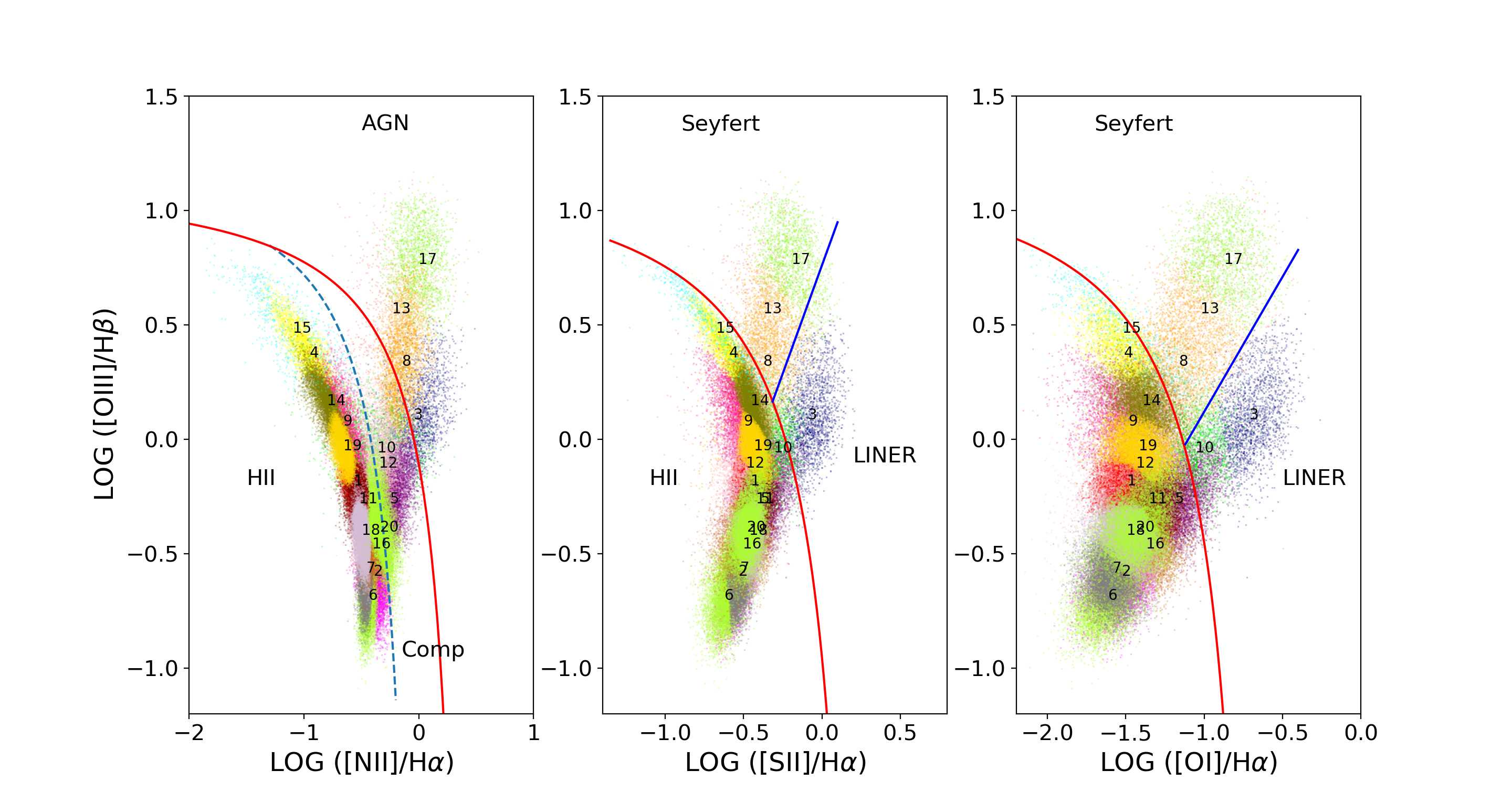
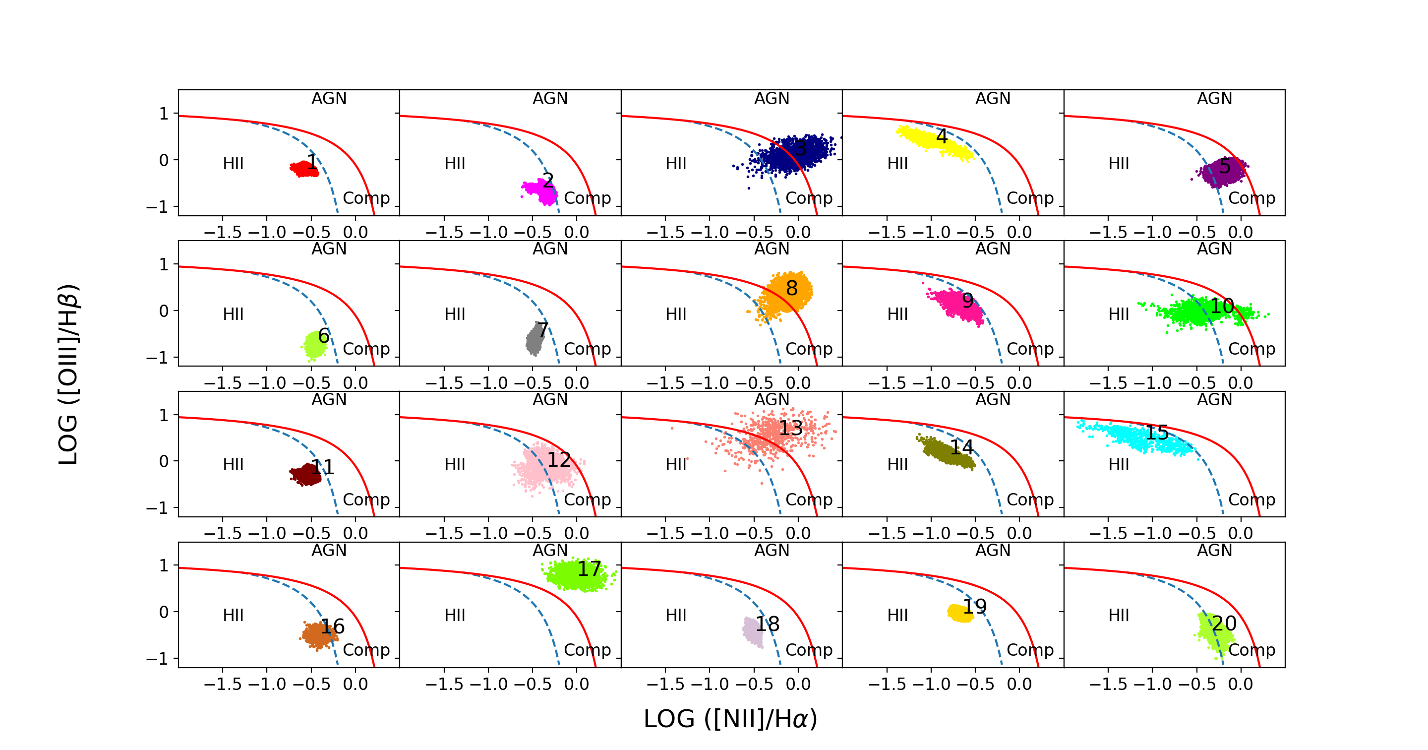
Figure 10: The top panel shows the BPT diagnostic diagrams for the SDSS DR8 sample with SNR$>$3 for all considered emission lines, including the [O i]$\lambda 6300$. Each galaxy is colour-coded according to its most probable allocation to one of the 20 subpopulations. The maximum ’starburst’ line of Kewley et al. (2001) is shown by the solid red line and the empirical upper bound on SFG of Kauffmann et al. (2003) is plotted as the dashed blue line. The empirical line for distinguishing Seyferts and LINERs of Kewley et al. (2006) is depicted by the solid blue line. The bottom panel shows the 20 subpopulations plotted on the [N ii]$/$H$\alpha$ vs [O iii]$/$H$\beta$ projection of the 4-dimensional diagnostic diagram. The subpopulations are numbered following the scheme in the top panel. This figure shows the spatial extent of each subpopulation and their location with respect to the standard diagnostic lines in the [O iii]$/$H$\beta$ diagram. Since these are 2-dimensional projections of the 4-dimensional distribution in each subpopulation, they only give an indication of the extent and location of each subpopulation.

Table 9: A 3-way classification table that compares the SoDDA classification of the filtered sample with the standard, 2-dimensional classification scheme (Kewley et al., 2006). Each cell has 3 values: the number of galaxies with (i) $\rho_{ic}^{\rm filter}\geq 75\%$, (ii) $50\%\leq\rho_{ic}^{\rm filter}<75\%$, and (iii) $\rho_{ic}^{\rm filter}<50\%$, where $\rho_{ic}^{\rm filter}$ is the posterior probability that galaxy $i$ belongs to galaxy class $c$ under SoDDA filtered. blackContradictory classifications are called ambiguous classifications by Kewley et al. (2006).

SoDDA filtered	Kewley et al. (2006)
		SFGs				Seyferts				LINERs				Comp				Contradictory				Total
		$\geq 75\%$	$50\%-75\%$	$<50\%$		$\geq 75\%$	$50\%-75\%$	$<50\%$		$\geq 75\%$	$50\%-75\%$	$<50\%$		$\geq 75\%$	$50\%-75\%$	$<50\%$		$\geq 75\%$	$50\%-75\%$	$<50\%$		$\geq 75\%$	$50\%-75\%$	$<50\%$
	SFGs	73414	2338	25		0	0	0		0	0	0		1973	1552	28		850	151	7		76237	4041	60
	Seyferts	33	15	3		3432	3	0		41	66	11		612	564	16		848	108	10		4966	756	40
	LINERs	0	0	0		0	0	0		965	198	26		466	172	16		43	39	5		1474	409	47
	Comp	392	933	27		0	0	0		3	45	9		4908	2719	49		427	252	15		5730	3949	100

Table 10: Comparison of the SoDDA classification of the filtered sample (SNR$>3$ on all considered diagnostic lines) with that of the SoDDA classification of the sample considered in SS3. The classification is performed in the ([O iii]$/$H$\beta$, [N ii]$/$H$\alpha$, [S ii]$/$H$\alpha$ and [O i]$/$H$\alpha$) space.

SoDDA filter	SoDDA
		SFGs	Seyferts	LINERs	Composites	Total
	SFGs	78525	0	1	1812	80338
	Seyferts	131	4751	45	835	5762
	LINERs	18	10	1757	145	1930
	Composites	1698	12	110	7959	9779
	Total	80372	4773	1913	10751

Appendix B Online Material

In the online version of this article, we provide the following:

1. Tables in numpy format including the estimated mean $\mu_{k}$, covariance matrix $\Sigma_{k}$, and the weight $\pi_{k}$ for each subpopulation $k=1,...,20$ (named means.npy, covars.npy, and weights.npy respectively). These are the definitions of the clusters as derived from the analysis presented is Section 3.

2. blackTables in numpy format including the estimated mean $\mu_{k}$, covariance matrix $\Sigma_{k}$, and the weight $\pi_{k}$ for each subpopulation $k=1,...,20$ (named m_filter.npy, c_filter.npy, and w_filter.npy respectively). These are the definitions of the clusters as derived from the analysis presented is Appendix A for the filtered sample.

3. Tables in numpy format providing the coefficients and the intercepts for the 4-dimensional (named svm_4d_coefs.npy and svm_4d_intercept.npy) and the 3-dimensional (named svm_3d_coefs.npy and svm_3d_intercept.npy respectively) surfaces based on the SVM method (Eqs. 12–23, and 24-35 respectively). These are the definitions of the surfaces as derived from the analysis presented is Section 4. blackWe also include the trained SVM model, estimated using the scikit-learn Python library, for both the 4-dimensional (svm_4d.sav) and the 3-dimensional (svm_3d.sav) case.

4. A python script (classification.py) that allows the reader to directly apply the SoDDA and the SVM classification based blackon the clusters and the separating surfaces, respectively, derived in Sections 3 and 4. It contains a function that given the 4 emission-line ratios $\log($[N ii]$/$H$\alpha$), $\log$([S ii]$/$H$\alpha$), $\log$([O i]$/$H$\alpha$) and $\log$([O iii]$/$H$\beta$), it computes the posterior probability of belonging to each of the 4 activity classes (SFGs, Seyferts, LINERs, and Composites blackfor class 0, 1, 2, and 3, respectively). We also include two functions which give the classification of a galaxy based on the 4-dimensional and the 3-dimensional SVM surfaces given its 4 emission line ratios.

5. blackA Readme file that explains the arguments and the output of the functions in the python script (classification.py) and contains examples of using them on sample data.

6. blackA table (data_classified.csv) that contains the SoDDA-based probability that each galaxy belongs to each one of the activity classes, derived in the analysis presented in Section 3. It also includes the galaxy’s SPECOBJID, the key diagnostic line-ratios, and the activity classification based on the class with the highest probability.

References

- Aihara et al. (2011a) Aihara H., et al., 2011a, ApJS, 193, 29
- Aihara et al. (2011b) Aihara H., et al., 2011b, ApJS, 195, 26
- Baldwin et al. (1981) Baldwin J. A., Phillips M. M., Terlevich R., 1981, PASP, 93, 5
- Bilmes et al. (1998) Bilmes J. A., et al., 1998, International Computer Science Institute, 4, 126
- Brinchmann et al. (2004) Brinchmann J., Charlot S., White S. D. M., Tremonti C., Kauffmann G., Heckman T., Brinkmann J., 2004, MNRAS, 351, 1151
- Cid Fernandes et al. (2011) Cid Fernandes R., Stasińska G., Mateus A., Vale Asari N., 2011, MNRAS, 413, 1687
- Cortes & Vapnik (1995) Cortes C., Vapnik V., 1995, Machine learning, 20, 273
- Dale et al. (2006) Dale D. A., et al., 2006, ApJ, 646, 161
- Dempster et al. (1977) Dempster A. P., Laird N. M., Rubin D. B., 1977, Journal of the royal statistical society. Series B (methodological), pp 1–38
- Donley et al. (2012) Donley J. L., et al., 2012, ApJ, 748, 142
- Eisenstein et al. (2011) Eisenstein D. J., et al., 2011, AJ, 142, 72
- Ferland (2003) Ferland G. J., 2003, ARA&A, 41, 517
- Fraley & Raftery (2002) Fraley C., Raftery A. E., 2002, Journal of the American statistical Association, 97, 611
- Groves et al. (2012) Groves B., Brinchmann J., Walcher C. J., 2012, MNRAS, 419, 1402
- Heckman (1980) Heckman T. M., 1980, A&A, 87, 152
- Ho et al. (1997) Ho L. C., Filippenko A. V., Sargent W. L. W., Peng C. Y., 1997, ApJS, 112, 391
- Juneau et al. (2011) Juneau S., Dickinson M., Alexander D. M., Salim S., 2011, ApJ, 736, 104
- Juneau et al. (2014) Juneau S., et al., 2014, ApJ, 788, 88
- Kauffmann et al. (2003) Kauffmann G., et al., 2003, MNRAS, 346, 1055
- Kewley et al. (2001) Kewley L. J., Dopita M. A., Sutherland R. S., Heisler C. A., Trevena J., 2001, ApJ, 556, 121
- Kewley et al. (2006) Kewley L. J., Groves B., Kauffmann G., Heckman T., 2006, MNRAS, 372, 961
- Kewley et al. (2013) Kewley L. J., Maier C., Yabe K., Ohta K., Akiyama M., Dopita M. A., Yuan T., 2013, ApJ, 774, L10
- Kormendy & Ho (2013) Kormendy J., Ho L. C., 2013, ARA&A, 51, 511
- Mukherjee et al. (1998) Mukherjee S., Feigelson E. D., Jogesh Babu G., Murtagh F., Fraley C., Raftery A., 1998, ApJ, 508, 314
- Rich et al. (2014) Rich J. A., Kewley L. J., Dopita M. A., 2014, ApJ, 781, L12
- Schwarz et al. (1978) Schwarz G., et al., 1978, The annals of statistics, 6, 461
- Shi et al. (2015) Shi F., Liu Y.-Y., Sun G.-L., Li P.-Y., Lei Y.-M., Wang J., 2015, Monthly Notices of the Royal Astronomical Society, 453, 122
- Spinoglio & Malkan (1992) Spinoglio L., Malkan M. A., 1992, ApJ, 399, 504
- Stasińska et al. (2006) Stasińska G., Cid Fernandes R., Mateus A., Sodré L., Asari N. V., 2006, MNRAS, 371, 972
- Stasińska et al. (2015) Stasińska G., Costa-Duarte M. V., Vale Asari N., Cid Fernandes R., Sodré L., 2015, MNRAS, 449, 559
- Stern et al. (2005) Stern D., et al., 2005, ApJ, 631, 163
- Tibshirani et al. (2001) Tibshirani R., Walther G., Hastie T., 2001, Journal of the Royal Statistical Society: Series B (Statistical Methodology), 63, 411
- Tommasin et al. (2010) Tommasin S., Spinoglio L., Malkan M. A., Fazio G., 2010, ApJ, 709, 1257
- Tremonti et al. (2004) Tremonti C. A., et al., 2004, ApJ, 613, 898
- Veilleux & Osterbrock (1987) Veilleux S., Osterbrock D. E., 1987, ApJS, 63, 295
- Vogt et al. (2014) Vogt F. P. A., Dopita M. A., Kewley L. J., Sutherland R. S., Scharwächter J., Basurah H. M., Ali A., Amer M. A., 2014, ApJ, 793, 127
- Weiner et al. (2007) Weiner B. J., et al., 2007, ApJ, 660, L39
- Wolfe (1970) Wolfe J. H., 1970, Multivariate Behavioral Research, 5, 329
- Yan et al. (2011) Yan R., et al., 2011, ApJ, 728, 38
- York et al. (2000) York D. G., et al., 2000, AJ, 120, 1579
- Yuan et al. (2010) Yuan T.-T., Kewley L. J., Sanders D. B., 2010, ApJ, 709, 884
- de Souza et al. (2017) de Souza R. S., et al., 2017, MNRAS, 472, 2808
Appendix A \colorblackAnalysis of the SDSS Data Release 8 sample with SNR3 for [O i]