MIMO with Energy Recycling

Abstract

We consider a Multiple Input Single Output (MISO) point-to-point communication system in which the transmitter is designed such that, each antenna can transmit information or harvest energy at any given point in time. We evaluate the achievable rate by such an energy-recycling MISO system under an average transmission power constraint. Our achievable scheme carefully switches the mode of the antennas between transmission and wireless harvesting, where most of the harvesting happens from the neighboring antennas’ transmissions, i.e., recycling. We show that, with recycling, it is possible to exceed the capacity of the classical non-harvesting counterpart. As the complexity of the achievable algorithm is exponential with the number of antennas, we also provide an almost linear algorithm that has a minimal degradation in achievable rate. To address the major questions on the capability of recycling and the impacts of antenna coupling, we also develop a hardware setup and experimental results for a 4-antenna transmitter, based on a uniform linear array (ULA). We demonstrate that the loss in the rate due to antenna coupling can be made negligible with sufficient antenna spacing and provide hardware measurements for the power recycled from the transmitting antennas and the power received at the target receiver, taken simultaneously. We provide refined performance measurement results, based on our actual measurements.

I Introduction

When information is transmitted wirelessly, only a small fraction of the emitted power reaches the intended receive antenna. Energy recycling is based on the premise that some of the emitted energy can be captured back and reused by the transmitter itself. In principle, a wireless transmitter equipped with energy harvesting capabilities may benefit, not only from other natural and man-made sources of wireless energy [1], but also from its own transmitted power. Indeed, if done properly, this provides a significant improvement over wireless energy transfer, since the power is captured from a nearby antenna, where the power received can be orders of magnitude higher than the power that can be received from a far away station.

Energy recycling is particularly a good fit for Multi Input Multi Output (MIMO) communication due to the potentially large number of antennas to harvest from. Indeed, with transmit beamforming, due to spatial diversity, the transmission power over each antenna can vary substantially. Therefore, at any given time, the contribution of different transmission antennas to the achieved rate can be different. If the transmit antennas can switch between two modes, signal transmission and energy harvesting, we can use antennas with relatively low contribution at a time to energy harvesting mode. The hypothesis is that, by doing so, the savings in average power can make up for the minimal loss due to not transmitting over that antenna at that time. In this paper, we show that this is indeed the case and with a careful control of switching between harvesting and transmission modes, for a given average transmission power constraint, the achievable rate can be higher than the capacity of the classical MIMO system without energy recycling. Unlike most of the available literature, we are concerned with the opportunity of energy recycling at the transmitter side rather than harvesting it at the receiver side.

We study a Multi Input Single Output (MISO) point-to-point communication model in which, at any given point in time, the transmitter deactivates a subset of its transmitting antennas and assigns them for energy harvesting. The energy harvested over these antennas is then recycled and can be reused by the transmitter, see Figure (1). We study the information-theoretic limits of the aforementioned harvesting MISO system in terms of its achievable communication rate. We show that the rate achievable by the energy-recycling MISO system is above the capacity of the conventional MISO system without recycling, with an increasing margin as the number of antennas increase. Our achievable scheme includes an antenna scheduling algorithm that determines which antennas should be active as a function of the antenna-to-antenna loss gains at the transmitter and the transmitter-to-receiver channel gains. The complexity of the developed optimal antenna scheduling algorithm is found to grow exponentially with the number, $M$, of the transmitter antennas. To address this problem, we provide $O(M\log M)$ complexity algorithm, which achieves the optimal performance in a symmetric system, where the propagation loss between each pair of transmission antennas is identical. Although we considered a MISO channel for the sake of simplicity of the exposure of the ideas, the analysis conducted can be generalized to a MIMO setting in a straightforward fashion.

One of the main questions around energy recycling is its practicality in real situations. The major problem here is, due to antenna coupling, the harvesting antennas affect the energy received by the receive antennas in the far field. To understand the severity of this problem, we conduct hardware experiments using universal serial radio peripheral (USRP) devices. Clearly, the closer the harvesting antenna to an active one, the higher the harvested energy. While understanding this behavior, our experiments reveal the amount of decrease in the power at the target receiver. We experimentally identify the optimal tradeoff between the harvested and the received power for uniform linear arrays (ULA) at the transmitter. We show that, the best recycling-receive power tradeoff is observed when the antenna-spacing in the array is identical to a quarter wavelength.

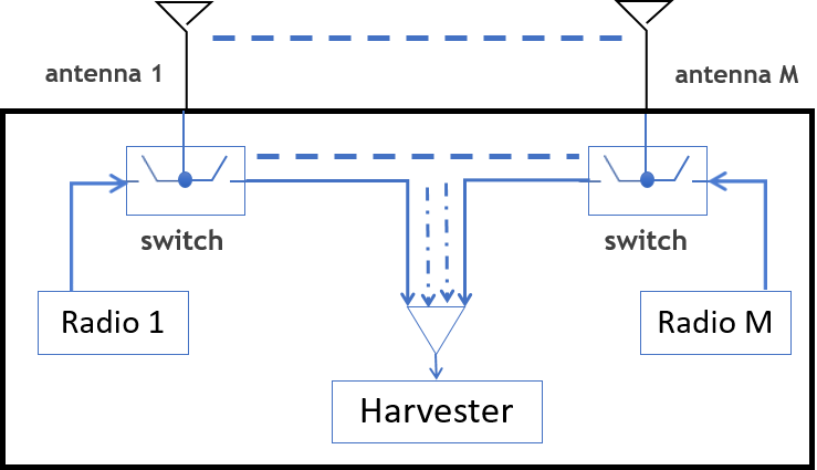
Figure 1: Transmitter with $M$ antennas. The switches control the role of each antenna, as they can actively transmit the signal fed by the radio or harvest ambient energy, a large portion of which comes from actively-transmitting antennas.

Several research efforts are made to develop communication schemes for networks composed of energy harvesting nodes, equipped with a single antenna. The fundamental tradeoff between the rates at which energy and reliable information can be transmitted over a single noisy line is studied in [2]. In [3], the problem of wireless information and power transfer across a noisy coupled-inductor circuit, which is a frequency-selective channel with additive white Gaussian noise. The optimal tradeoff between the achievable rate and the power transferred is characterized given the total power available. Several other works considering, mainly, the optimal control policy for networks with energy harvesting nodes can be found in the literature, see e.g. [4, 5, 6, 7, 8, 9, 10, 11, 12, 13]. Simultaneous energy and information transfer literature has been extended to MIMO broadcast [14], fading [15] and interference [16] channels.

To our best knowledge, this is the first study that considers the basic limits of wireless communication with energy recycling. Along with providing efficient resource allocation schemes with almost capacity-achieving performance, the other unique feature of our study is that, we provide a thorough evaluation of the concept of energy recycling using an actual hardware setup with USRPs.

II System Model

We consider a point-to-point MISO communication in which a transmitter equipped with $M$ antennas wishes to send a message to a receiver with a single antenna. In our system, at any given point in time, a selected subset of the antennas may not transmit. Instead they harvest wireless energy, a substantial portion of which is coming from the active antennas. We call this communication model recycling MISO. This is unlike the traditional non-recycling MISO communication [17, 18], where each antenna can only be in the transmission mode. In our system, the antennas that transmit are referred to as active and the antennas that remain silent and harvest energy are referred to as harvesting.

Let $\mathcal{A}$ be the set that denotes indices of the active antennas at the transmitter at a particular channel use. Then, the observed signal at harvesting antenna $l$ of the transmitter at that channel use can be written as

$$Z_{l}=\sum_{k\in\mathcal{A}}\sqrt{\alpha_{kl}}X_{k}+N_{l},$$ (1)

where $X_{k}$ is the complex transmitted signal at active antenna $k$, $\alpha_{kl}$ is the path loss of the channel connecting $k$-th antenna to $l$-th antenna (both at the transmitter), and $N_{l}$ is the additive noise signal, distributed as $\mathcal{CN}(0,1)$. The corresponding harvested energy for $Z_{k}$ is $|Z_{k}|^{2}$. Note that $\{\alpha_{kl}\}_{k,l\in\mathcal{M}}$ depend on the geometry of antenna placements at the transmitter, where $\mathcal{M}\triangleq\{1,\ldots,M\}$. As seen in (1), in the recycling MISO communication, passive antennas harvest energy using the incoming signal from their active neighboring antennas.

We assume a flat fading transmitter-to-receiver channel, in which the channel gains in different channel uses are identically and independently distributed (i.e., rich scattering is present between the transmitter and the receiver). This assumption is merely for the simplicity of the analysis, but generalization to other propagation settings is straightforward. The observed signal at the single receive antenna at a particular channel use can be written as

$$Y_{k}=\sum_{k\in\mathcal{A}}X_{k}G_{k}+W,$$ (2)

where $Y_{k}$ is the received complex signal and $W$ is the additive noise signal, distributed as $\mathcal{CN}(0,1)$. In the above equation, $G_{k}$ is the complex gain of the channel connecting the $k$-th antenna at transmitter to the receiver. We assume that the channel gains $G\triangleq[G_{1},\ldots G_{M}]$ are independent through space and are distributed as $\mathcal{CN}(0,I_{M})$, where $I_{M}$ is $M\times M$ identity matrix and parameter $d$ denotes the path loss gain of the channel between the transmitter and the receiver.

In this paper, we consider that full channel state information (CSI) is available, where both transmitter and the receiver have the perfect information of the channel gains. Hence, the transmitter has the ability to choose active and passive antennas as well as the transmission power as a function of the instantaneous channel gains. We develop antenna scheduling algorithm that determines which antennas should be active as a function of the antenna-to-antenna loss gains $\{\alpha_{kl}\}_{k,l=1,\ldots,M}$ at the transmitter and the channel gains. For the active antennas, we evaluate the capacity-achieving power allocation. Ultimately, we compare the achievable rates with and without recycling, subject to an average energy constraint.

III Basic Limits of Energy-Recycling MISO

In this section, we evaluate a rate that is achievable with our energy-recycling MISO communication system. We also provide the associated antenna scheduling and power allocation schemes that maximize this rate.

III-A Basic Limits

First, we state the capacity of the classical no-recycling MISO communication [18, 17] with the channel model we presented in the previous section:

$$C_{\text{no-ryc}}= \max_{P(\cdot)}\mathbb{E}\left[\log\left(1+P(H)\sum_{k=1}^{M}H_{k}\right)\right]$$ (3)

$$\text{subject to}\ \mathbb{E}\left[P(H)\right]\leq P_{c}$$ (4)

where $P_{c}$ is positive real number that denotes the average power constraint, $H_{k}\triangleq|G_{k}|^{2}$ denotes the power gain of the channel connecting $k$-th antenna at the transmitter to the receiver, and $H\triangleq\left[H_{1},\ldots,H_{M}\right]$. In (3), $P(\cdot):\mathbb{R}_{+}^{M}\to\mathbb{R}_{+}$ denotes the power allocation function, where $\mathbb{R}_{+}$ denotes all non-negative real numbers. Note that, here the average power constraint is a long-term average across time, summed over all transmission antennas.

The associated capacity-achieving power allocation function can be found to be the water-filling solution:

$$P(h)=\left(\lambda-\frac{1}{\sum_{k=1}^{M}h_{k}}\right)^{+},$$ (5)

where $h\triangleq[h_{1},\ldots,h_{M}]$ is the channel power gain sequence and $\lambda$ is non-negative real number that is chosen such that $\mathbb{E}\left[P(H)\right]=P_{c}$. Note that, Eq. (5) provides the total power allocation over all antennas at a given point, $k$, in time. The distribution of power across antennas to achieve the capacity given in (3) is found to be conjugate beamforming, which leads to the following transmitted signal vector across the antennas:

$$\mathbf{X}=\frac{G^{*}}{||G||}\cdot s,$$

where $s$ is the complex data signal.

Our first theorem provides a rate achievable with energy-recycling MISO communication. Subsequently, we compare the achievable rate with the capacity, (3), of the classical non-recycling system.

Theorem 1.

The following rate is achievable with MISO harvesting communication:

$$R_{\text{ryc}}= \max_{\mathcal{A}(\cdot),P(\cdot)}\mathbb{E}\left[\log\left(1+P(H)\sum_{k\in\mathcal{A}(H)}H_{k}\right)\right]$$ (6)

$$\text{subject to}\ \mathbb{E}\left[P(H)f(H)\right]\leq P_{c},$$ (7)

where $\mathcal{A}(\cdot)$ is a mapping from $M$ dimensional non-negative real space $\mathbb{R}_{+}^{M}$ to a non-empty subset of $\mathcal{M}$ and function $f(\cdot):\mathbb{R}_{+}^{M}\to\mathbb{R}_{+}$ is identical to:

$$f(h)=\left(1-\frac{\sum_{k\in\mathcal{A}(h)}\sum_{l\in\mathcal{A}^{c}(h)}h_{k}\alpha_{kl}}{\sum_{k\in\mathcal{A}(h)}h_{k}}\right).$$

for any $h\in\mathbb{R}_{+}^{M}$.∎

The proof of Theorem 1 can be found in Appendix A. In Theorem 1, subset $\mathcal{A}(h)\subseteq\mathcal{M}$ denotes the set of active antennas for channel power sequence $h$. The transmitter keeps the antennas in subset $\mathcal{A}^{c}(h)$ in the harvesting mode in order to harvest energy using the signal coming from the active antennas in set $\mathcal{A}(h)$. In order to achieve rate (6), the transmitter employs conjugate beamforming across the active antennas, similar to the non-recycling setting. Also, observe that, the average power constraint is on the consumed energy rather than the transmitted energy. For example, suppose the average power constraint is $1$mW, we allow our transmitters to transmit an average power of $1.1$mW if an average power of $0.1$mW is recycled back into the batteries.

Remark 1.

One can observe that $R_{\text{ryc}}\geq C_{\text{no-ryc}}$: Let $\mathcal{A}(h)=\mathcal{M}$ for any $h\in\mathbb{R}_{+}^{M}$. Then, $f(h)=1$ for any $h$ and the optimization problem in (6) becomes equal to that in (3).∎

III-B Optimal Antenna Scheduling and Power Allocation

We next find a power allocation function $P(\cdot)$ and mapping $\mathcal{A}(\cdot)$ solving the optimization problem in (6). Define power allocation function $P_{\text{new}}(\cdot):\mathbb{R}_{+}^{M}\to\mathbb{R}_{+}$ as

$$P_{\text{new}}(h)\triangleq P(h)f(h)$$

for any $h\in\mathbb{R}_{+}^{M}$. We can write the optimization problem in (6) in terms of $P_{new}(\cdot)$ as

$$\begin{aligned} R_{\text{ryc}}=&\max_{\mathcal{A}(\cdot),P(\cdot)}\mathbb{E}\left[\log\left(1+P_{\text{new}}(H)g_{\mathcal{A}}(H)\right)\right]\\ &\text{subject to}\ \mathbb{E}\left[P_{\text{new}}(H)\right]\leq P_{c}\end{aligned}$$ (8)

where function $g_{\mathcal{A}}(\cdot):\mathbb{R}_{+}^{M}\to\mathbb{R}_{+}$ is defined as

$$g_{\mathcal{A}}(h)\triangleq\frac{\sum_{k\in\mathcal{A}(h)}h_{k}}{f_{\mathcal{A}}(h)}=\frac{(\sum_{k\in\mathcal{A}(h)}h_{k})^{2}}{\sum_{k\in\mathcal{A}(h)}h_{k}-\sum_{k\in\mathcal{A}(h)}\sum_{k\in\mathcal{A}^{c}(h)}h_{k}\alpha_{kl}}$$

for any mapping $\mathcal{A}(\cdot):\mathbb{R}_{+}^{M}\to\mathbb{M}$. Notice that, in (8), the maximization is over $P(\cdot)$. Hence replacing $P(\cdot)$ with $P_{\text{new}}(\cdot)$ does not change the value of the optimization problem. We can rewrite the optimization problem in (8) as

$$\begin{aligned} R=&\max_{\mathcal{A}(\cdot),P_{\text{new}}(\cdot)}\mathbb{E}\left[\log\left(1+P_{\text{new}}(H)g_{\mathcal{A}}(H)\right)\right]\\ &\text{subject to}\ \mathbb{E}\left[P_{\text{new}}(H)\right]\leq P_{c}.\end{aligned}$$ (9)

We next provide mapping $\mathcal{A}(\cdot)$ that solves (9). First note that for any power allocation function $P_{\text{new}}(\cdot)$ and mapping $\mathcal{A}(\cdot):\mathbb{R}_{+}^{M}\to\mathbb{M}$, inner maximization in (9) is bounded as

$$\mathbb{E}\left[\log\left(1+P_{\text{new}}(H)g_{\mathcal{A}}(H)\right)\right]\\ \leq\mathbb{E}\left[\log\left(1+P_{\text{new}}(H)g_{\text{max}}(H)\right)\right],$$ (10)

where $g_{max}(H)\triangleq\max_{\mathcal{A}}g_{\mathcal{A}}(H)$. Hence, mapping $\mathcal{A}_{\text{max}}(\cdot)$, defined as

$$\mathcal{A}_{\text{max}}(h)\triangleq\arg\max_{\mathcal{A(\cdot)}}g_{\mathcal{A}}(h)$$

for all $h\in\mathbb{R}_{+}$ solves the optimization problem in (9). We conclude that $A_{\text{m}ax}(h)$ is the set of antennas that the transmitter schedules as active for channel power sequence $h$ in order to achieve the rate proposed in Theorem 1.

Replacing the inner maximization in (9) with the expectation term in (10) leads to the following optimization problem:

$$\begin{aligned} R_{ryc}=&\max_{P_{\text{\text{new}}}(\cdot)}\mathbb{E}\left[\log\left(1+P_{\text{\text{new}}}(H)g_{\text{max}}(H)\right)\right]\\ &\text{subject to}\ \mathbb{E}\left[P_{\text{new}}(H)\right]\leq P_{c}.\\ \end{aligned}$$ (11)

The power allocation function that solves the optimization problem in (11) has the water-filling form, given by:

$$P_{\text{\text{new}}}(h)=\left(\lambda-\frac{1}{g_{\text{max}}(h)}\right)^{+},$$

where $\lambda$ is non-negative real number that is chosen such that $\mathbb{E}\left[P_{\text{new}}(H)\right]=P_{c}$.

III-C Low-complexity Near-Optimal Antenna Scheduling and Power Allocation

Note that in order to find the active antennas at given channel power gain vector $h$, the transmitter needs to find $\mathcal{A}_{\text{max}}(h)$. Since there are $2^{M}-1$ non-zero subsets of $\mathcal{M}$, the antenna scheduling process will take a time that varies exponentially with the number of antennas, $M$.

To address this complexity issue, we next provide an algorithm for computing the active antenna set, $\mathcal{A}_{\text{m}ax}(h)$ for a given channel power sequence $h=[h_{1},\ldots,h_{M}]$, with a time complexity that scales as $O(M\log M)$. We also show that the low-complexity antenna scheduler is optimal when all coefficients $\{\alpha_{kl}\}_{k,l=1,\ldots M}$ are identical.

Suppose that $\alpha_{kl}=\alpha$ for any $k,l\in\mathcal{M}$. Mapping $g_{\mathcal{A}}(h)$ reduces to:

$$g_{\mathcal{A}}(h) =\frac{(\sum_{k\in\mathcal{A}(h)}h_{k})^{2}}{\sum_{k\in\mathcal{A}(h)}h_{k}-\sum_{k\in\mathcal{A}(h)}\sum_{l\in\mathcal{A}(h)^{c}}h_{k}\alpha}$$

$$=\frac{\sum_{k\in\mathcal{A}(h)}h_{k}}{1-(M-|\mathcal{A}(h)|)\alpha}.$$ (12)

Suppose that $\{h_{n_{k}}\}_{k\in\{1,\dots,M\}}$ is a channel power sequence sorted in a descending order such that $h_{n_{k}}\geq h_{n_{k+1}}$ for all $k\in{1,\ldots M-1}$. We define function $g_{i}(\cdot):\mathbb{R}_{+}^{M}\to\mathbb{R}_{+}$ as

$$g_{i}(h)\triangleq\frac{\sum_{k=1}^{i}h_{n_{k}}}{1-(M-i)\alpha}.$$

Note that $g_{i}(h)=g_{\mathcal{A}}(h)$ for $\mathcal{A}(h)=\{n_{1},\dots n_{i}\}$ due to definition above and (12). Further,

$$g_{i}(h)=\max_{\{\mathcal{A}(\cdot)\ \left|\ |\mathcal{A}(h)|=i\right.\}}g_{\mathcal{A}}(h)$$

due to the fact that $\{h_{n_{1}},h_{n_{2}},\ldots,h_{n_{i}}\}$ are the $i$ largest channel power gains in $h$. Then, we can write the following:

$$\max_{i\in\mathcal{M}}g_{i}(h) =\max_{i\in\mathcal{M}}\max_{\{\mathcal{A}(\cdot)\ \left|\ |\mathcal{A}(h)|=i\right.\}}g_{\mathcal{A}}(h)$$

$$=\max_{\mathcal{A}(\cdot)}g_{\mathcal{A}}(h).$$

Defining $i^{*}\triangleq\arg\max_{i\in\mathcal{M}}g_{i}(h)$, we conclude that $\{n_{1},\dots n_{i^{*}}\}=\mathcal{A}_{\text{m}ax}(h)$. Hence, once the transmitter computes index $i^{*}$, it finds which antennas to keep active. Exploiting the fact that all $\alpha_{kl}$’s are identical, we converted the problem $\arg\max_{\mathcal{A}(\cdot)}g_{\mathcal{A}}(h)$ into a simpler problem $\arg\max_{i}g_{i}(h)$. The time complexity of solving the first problem is $O(2^{M})$ due to the fact there are $2^{M}-1$ non-empty subset of $\mathcal{M}$. On the other hand, solving the second problem has a time complexity of $O(M)$.

Furthermore, the transmitter does not even need to compute all $g_{i}(h)$’s in order to find index $i^{*}$. Next lemma clarifies this proposition.

Lemma 1.

For any $h\in\mathbb{R}_{+}^{M}$, if there exists $i\in\{1,\ldots,M-1\}$ such that $g_{i}(h)\geq g_{i+1}(h)$, then $g_{i}(h)\geq g_{j}(h)$ for any $j$ such that $i\leq j\leq M$.

Proof.

Suppose there exists $i\in\{1,\ldots,M-1\}$ such that $g_{i}(h)\geq g_{i+1}(h)$. The inequality $g_{i}(h)\geq g_{i+1}(h)$ is equivalent to the following:

$$\alpha\sum_{k=1}^{i}h_{n_{k}}\geq h_{n_{i+1}}\cdot(1-(M-i)\alpha)$$ (13)

Pick an arbitrary integer $t$ such that $i+t\leq M$. Similarly, the inequality $g_{i}(h)\geq g_{i+t}(h)$ is equivalent to the following:

$$t\cdot\alpha\sum_{k=1}^{i}h_{n_{k}}\geq\sum_{k=i+1}^{i+t}h_{n_{k}}\cdot(1-(M-i)\alpha)$$ (14)

In order to prove Lemma 1, we need to show that the inequality in (13) implies the inequality in (14). Hence, assuming the inequality in (13) is true, we have the following:

$$t\cdot\alpha\sum_{k=1}^{i}h_{n_{k}} \geq t\cdot h_{n_{i+1}}(1-(M-i)\alpha)$$

$$\geq\sum_{k=i+1}^{i+t}h_{n_{k}}\cdot(1-(M-i)\alpha),$$

where the first inequality follows from the inequality in (13). The second inequality follows from the fact that $h_{n_{i+1}}\geq\max_{j:i+1\leq j\leq i+1}h_{n_{j}}$. ∎

We now provide the antenna scheduling algorithm. First the transmitter sorts the channel power sequence $\{h_{n_{k}}\}_{k\in\{1,\dots,M\}}$ in a descending order such that $h_{n_{k}}\geq h_{n_{k+1}}$ for all $k\in{1,\ldots M-1}$. Then, the transmitter evaluates $i^{*}=\arg\max_{i\in\mathcal{M}}g_{i}(h)$ using Lemma 1. More specifically, starting at $i=1$ and increasing $i$ by one at each step, the transmitter computes $g_{i}(h)$ until step $j$ where $g_{j}(h)\geq g_{j+1}(h)$. The transmitter sets $i^{*}$ to $j$. If there is no $i\in\{1,\ldots,M-1\}$ such that $g_{i}(h)\geq g_{i+1}(h)$, the transmitter sets $i^{*}$ to $M$. Finally, transmitter schedules antennas with indices $\{n_{1},\ldots,n_{i^{*}}\}$ as active antennas.

The steps of the algorithm are formally given below:

Algorithm 1 Antenna Scheduling

1:Sort $\{h_{n_{k}}\}_{k\in\{1,\dots,M\}}$$\triangleright$ such that $h_{n_{k}}\geq h_{n_{k+1}}$ for all $k\in{1,\ldots M-1}$

2:$i=1$

3:while $i<M$ and $g_{i}(h)<g_{i+1}(h)$  do $i=i+1$

4:end while

5:$\mathcal{A}_{\text{max}}(h)=\{n_{1},\ldots,n_{i}\}$

The time complexity of the above algorithm is $O(M\log M)$ since time complexity of sorting channel power sequence is $O(M\log M)$ and the time complexity of finding $i^{*}$ is $O(M)$.

IV Numerical Results

In this section we conduct simulations to illustrate the impact of harvesting on the achievable rate. Throughout the section, we take the mean path loss between the transmitter and the receiver as $-60$dB, i.e., $\mathbb{E}[H_{i}]=10^{-6}$ for all $i\in\mathcal{M}$. In some of our simulations, we impose a limit the maximum number of antennas that recycle energy at a given time in order to decrease the running time. We denote the maximum number of harvesting antennas as $M_{\text{harvest}}$. We also define antenna penalty as the number of antennas that we need to overcome not using recycling. For example, if the antenna penalty is $3$, it means the same rate as the non-recycling system can be achieved with $3$ less antennas with the recycling system.

In Figure 2, we plot rate $R_{ryc}$ achieved recycling MISO communication provided in Theorem 1 and the capacity of non-recycling MISO communication in (3) as a function of $M$ for different received signal to noise ratio (SNR) values. We set $M_{\text{harvest}}=5$ and all $\{\alpha_{i,j}\}_{i,j\in\mathcal{M}}$ to $-15$dB. Even though at most $5$ antennas are allowed to harvest, we observe that the rate gap between the harvesting and non-harvesting MISO communication widens as $M$ increases. The reason is that the number of options the transmitter has for selecting the harvesting antennas increases with $M$. The increased spatial diversity in the main channel provides an increased diversity in the choice of recycling antennas.

In Figure 2, we observe rate gains of $\%7$, $\%10$ and $\%20$ associated with recycling at SNR values $10$dB, $0$dB, and $-10$dB, respectively for a system size of $M=25$. Furthermore, the antenna penalty associated with the non-recycling system is larger than $3$, across all SNR values.

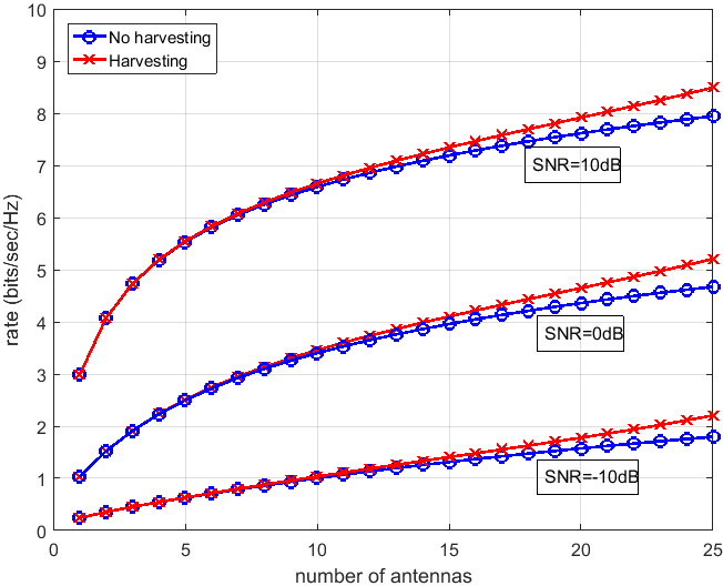
Figure 2: The variation of the achievable rate and the capacity at recycling and non-recycling MISO communications, respectively at different SNR values.

In Figure 3, we plot the rate achieved with recycling MISO communication as a function of $M_{\text{harvest}}$. We observe that achievable rate remains constant after $M_{\text{harvest}}$ exceeds $6$ antennas. The reason can be seen in Figure 4. In Figure 4, we plot the average number of harvesting antennas as a function of $M$. We observe that the average number of harvesting antennas is smaller than $6$ antennas for any $M$. Hence, picking $M_{\text{harvest}}$ greater than $6$ antennas will not bring an advantage.

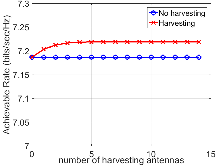
Figure 3: The variation of the rate achieved in recycling MISO communication as a function of number of maximum allowable harvesting antennas.

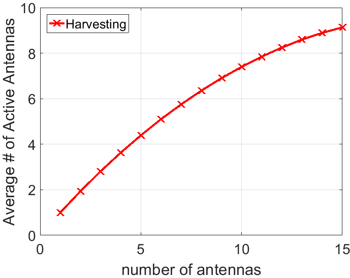
Figure 4: The variation of the average number of active (non-harvesting) antennas as a function of the total number of antennas at the transmitter

We next consider a particular geometry for placing antennas to the transmitter, as shown in Figure 5. Specifically, the antennas are placed on the center and the corners of each small hexagonal. The minimum distance between antennas is $\frac{\lambda}{3}$ that leads to $\alpha=10.3$dB (as per our hardware measurements as discussed in the next section), where $\lambda$ is the wavelength. We set $M_{\text{harvest}}$ to $6$ antennas and the received SNR to $10$dB. In Figure 6, we observe that antenna penalty associated with non-recycled transmitter is $4$ antennas at $M=20$.

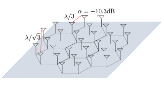
Figure 5: The placement of the transmitter antennas on a hexagonal grid. Each side of small hexagonals has a length of $\frac{\lambda}{3}$, where $\lambda$ is the wavelength.

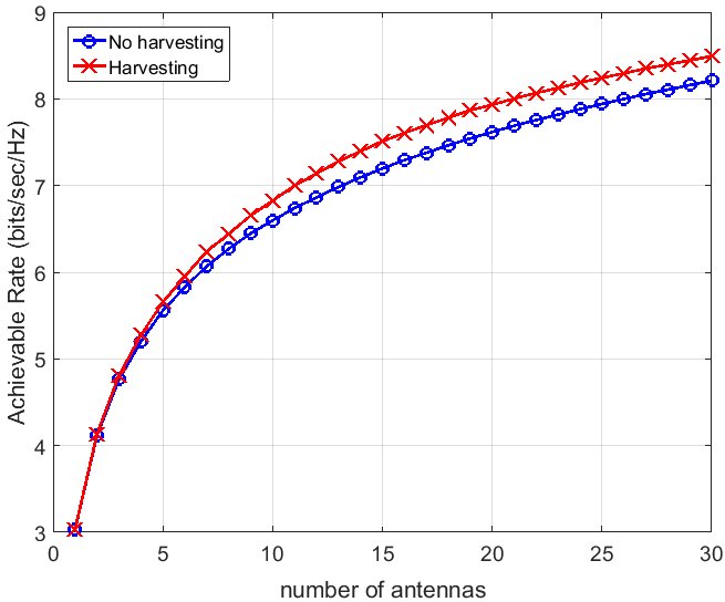
Figure 6: The variation of the achievable rate and the capacity at recycling and non-recycling MISO communications, respectively as a function of the total number of antennas at the transmitter.

V Hardware Measurements and Experimental Results

This section aims to address the questions around practicality of energy recycling. In particular, while having an inactive subset of the transmitter antenna array dedicated for energy harvesting, we study the trade-off between harvested and received power at the target receiver. While it can be expected that the closer the harvesting to the active antenna, the larger the power that can be harvested. Meanwhile, it is unclear how does this small separation affect the signal received at the target receiver affected by the coupling between transmission and harvesting antennas. Also, we aim to provide experimental results that shed the light on the selection of active and harvesting antennas. To that end, we use universal serial radio peripherals (USRP) to implement a MISO system with four elements uniform linear antenna array (ULA). First, we provide the hardware setup and the specification of the communication waveform used in these experiments. Then, we provide the experimental results for different selections of active and harvesting array subsets as a function of the array spacing.

V-A Hardware Setup

Hardware system components are listed in the Table I. Two CBX RF daughter boards from Ettus Research are installed in a single X300 USRP. Each RF daughter board has a single transmit single receive channels yielding a total of dual transmit dual receive channels. Our experiment goes by activating a maximum of two out of the four element antenna array while the remaining elements are dedicated for energy harvesting. The harvested and received power are measured using a stand alone spectrum analyzer. Figures 7 and 8 show the transmitter and spectrum analyzer used in our experiment.

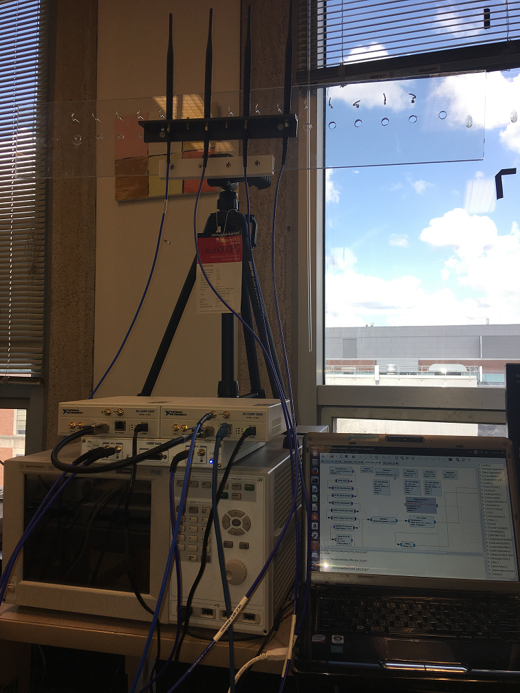
Figure 7: Ettus $X300$ with CBX daughter board takes the role of transmitter

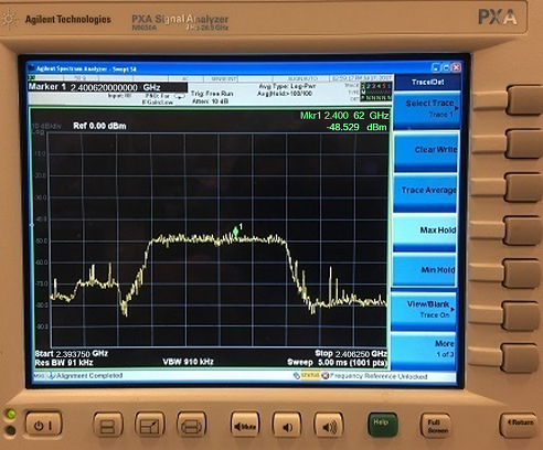
Figure 8: Spectrum analyzer used for power measurements. Center frequency $2.4GHz$, Signal bandwidth $5MHz$ , Resolution bandwidth $91KHz$.

TABLE I: List of Required Hardware Component.

Component	Type	Role in Experiment
CPU	Intel Core i5-3200 CPU 3.40GHz $\times$ 1	Host for signal processing
Operating System	Ubuntu 16.04 LTS, 64 bits	—
GNU Radio	Version 3.7.10	Signal Processing Environment
USRP	Ettus X300 $\times$ 1	Transmitter
RF Daughter Board	Ettus CBX $\times$ 2	Installed in one of the X300 USRP to form a dual channel Transmitter
Spectrum Analyzer	Agilent PXA	Placed 5 meters away from the transmitter

V-B Communication Setup

In our experimental setup, we have used IEEE-802.11p [19] signal waveform. We have used a slightly modified version of the GNU Radio based implementation of IEEE-802.11p provide in open source by the authors of [20]. Table II illustrates typical parameter values used in this experiment.

TABLE II: List of typical parameter values used in our experiment.

Parameter	Typical Value
Center Frequency	2.4 GHz
Bandwidth	5 MHz
FFT Length	64
Occupied Subcarrires	52
Data Subcarriers	48
Pilot Subcarriers	4
Packet Size	1000 Bytes
Packet Interval	150 ms
Transmit Power	+15 dBm
Array Configuration	ULA

V-C Results

First, we activate a single transmit antenna while keeping the other three antennas inactive. We measure the harvested power at each harvesting antenna as well as the power received by an antenna directly attached to the spectrum analyzer. The transmitter antenna array is $5$ meters away from the the spectrum analyzer. The spectrum analyzer provides the average power level measurements per resolution bandwidth. Denote by $P_{res}$, $W$ and $B$ the average power level per resolution bandwidth, the resolution bandwidth and the signal bandwidth, respectively. The total received power, $P_{t}$, is evaluated as follows:

$$P_{t}=10\log_{10}\left(\dfrac{B10^{(P_{res}/10})}{W}\right).$$ (15)

We have tested four different selections of active and harvesting antennas. As shown in Figure 9, we first activate the left most antenna while the remaining antennas are kept inactive for the sake of energy harvesting. Then, we used the second from the left antenna for data transmission. We then activate the two left most antennas and, finally, we use an interleaved pattern of harvesting and active antennas. At each setup, we measure the total harvested power and the power received at the target receiver for different array separations.

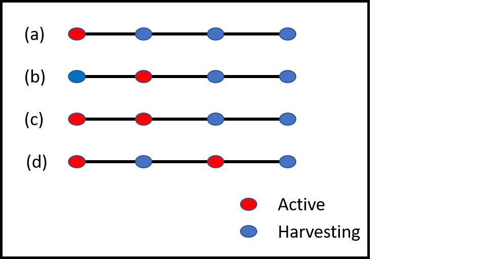
Figure 9: Illustration of our four selections of active and harvesting antennas.

We started by setting the array spacing equal to $\lambda/4$. In Figure 10, only the left most antenna is active while the remaining three antennas are dedicated for energy harvesting. We notice that, $\lambda/4$ element spacing yield the best harvesting performance. Meanwhile, the maximum received power is observed for array spacing of $\lambda/2$. Similar results can observed when the second left most antenna is used for transmission as can be seen in Figure 11. These results suggest that, the closer the harvesting antenna to the transmission antenna, the larger the energy that can be harvested, but also, the larger the coupling between transmission antennas and, hence, the less the power at the target receiver. It worth mentioning that, for array spacing less than $\lambda/4$, while a significant gain of harvesting energy was observed ($4$-$7$dBm), the average received power drops by $3$-$6$dBm due to coupling between the harvesting and transmission antennas.

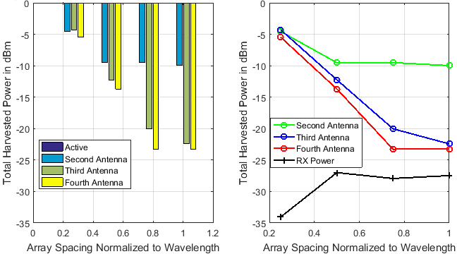
Figure 10: Total harvested and received power with the left most antenna active while the remaining elements are used for harvesting as a function of array spacing.

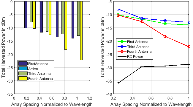
Figure 11: Total harvested and received power with the only the second antenna active while the remaining elements are used for harvesting as a function of array spacing.

In Figure 12, the two left most antennas are active. Again, we notice that, $\lambda/4$ element spacing yield the best harvesting performance. Meanwhile, the maximum is received power is, again, observed for array spacing of $\lambda/2$. On the other hand, in Figure 13, the two active antennas are chosen in an interleaved manner. In this setup, we notice that, $\lambda/4$ element spacing provide the best harvesting performance with relatively small reduction in the received power. The gain in harvesting energy is due to having the harvesting antennas closer to two active antennas while maintaining the spacing between the two active elements as $\lambda/2$. This gain comes at the expense of small reduction of received power due to coupling between harvesting and transmission antennas. Meanwhile, for larger array spacing, both the harvested and received power are reduced. This is due to the grating loops generated when the two active elements are separated. We see that the antenna that lies between two transmission antennas was able to maintain better harvesting energy.

The results of this section show that for the special case of a transmitter with ULA, the interleaved configuration with $\lambda/4$ element spacing provides significant gain in harvested energy and, at the same time, maintains reasonably small coupling loss. However, obviously in a rich scattering environment, any antenna spacing lower than $\lambda/2$ in the linear arrangement will lead to a reduction in the achieved spatial diversity. Thus, despite striking the optimal balance between recycled and received power, the small antenna spacing may lead to a decrease in the achieved rate in rich scattering environments.

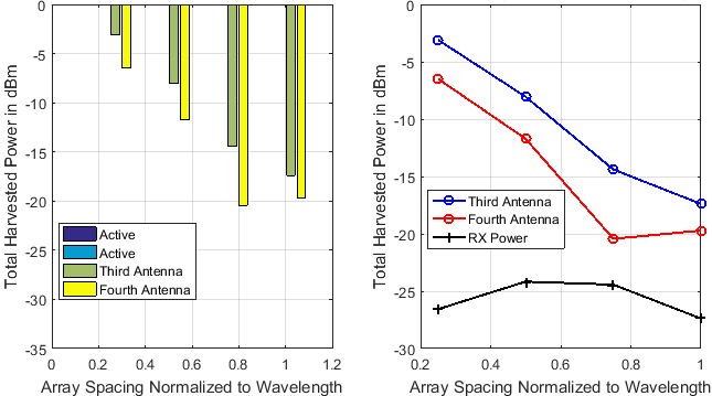
Figure 12: Total harvested and received power with the the two left most antennas are active while the remaining elements are used for harvesting as a function of array spacing.

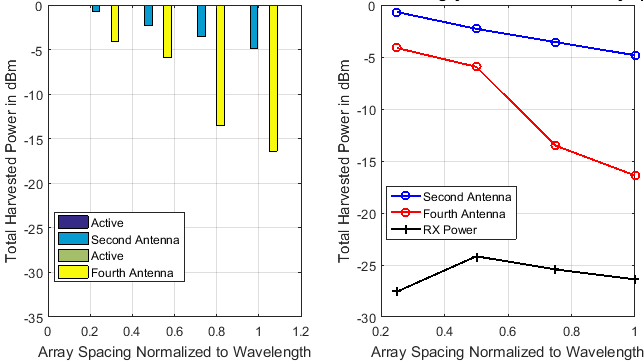
Figure 13: Total harvested and received power with the two active antennas selected in an interleaved manner while the remaining elements are used for harvesting as a function of array spacing.

VI Conclusion

We studied the basic limits of an energy recycling MISO communication system and showed that it can be utilized to increase the rate achieved, subject to an average power constraint. In our recycling setup, each transmission antenna can alternate between transmission and harvesting states, as chosen by the system. In this setting, we developed the capacity expression for the achievable rate with recycling. We developed the optimal antenna scheduling algorithm that decides on the active and recycling antennas. We also evaluated the optimal power allocation for the active antennas. However, we showed that the optimal scheme has a complexity that grows exponentially with the number of transmission antennas. To address this problem, we developed a near-optimal $O(M\log M)$ complexity algorithm, which preserves optimality in the case of symmetric gains between transmission-harvesting antenna pairs. We numerically evaluated the performance with energy recycling and showed that, with energy recycling, the number of antennas needed to achieve the same rate can be reduced by $10$-$15$% in typical cases.

To study the issues related to antenna coupling and understand the amount of reduction in received power, we developed a hardware setup and obtained experimental results for a $4\times 1$ MISO system with ULA at the transmitter. Our results reveal that, the closer the harvesting antenna to an active antenna, the larger the harvested power but also the larger the coupling between transmitting antennas, lowering the received power. For that setup, our evaluations showed that, having the transmitting and harvested antennas interleaved (one active followed by one harvesting antenna) at an array spacing equals to $\lambda/4$ yield the best harvested and received power results.

Appendix A Proof of Theorem 1

The transmitter employs Gaussian codebook and conjugate beamforming. The transmitted signal on active antennas can be written as

$$X=S\frac{G_{\mathcal{A}}^{*}}{||G_{\mathcal{A}}||}$$

where $G_{\mathcal{A}}\triangleq\{G_{k}\}_{k\in\mathcal{A}(H)}$. Note that $||G_{\mathcal{A}}||^{2}=\sum_{k\in\mathcal{A}(H)}H_{k}$. Furthermore, $S$ is complex Gaussian signal codeword signal at a particular channel use and is distributed as $CN(0,P(H))$

The rate for a given power allocation $P(\cdot)$ is mutual information $I(X;Y|H)$. We skip the derivation of equality

$$I(X;Y|H)=\mathbb{E}\left[\log\left(1+P(H)\sum_{k\in\mathcal{A}(H)}H_{k}\right)\right]$$

as the derivation is identical with the derivation of the capacity of the non-harvesting MISO communication proof of which can be found in [18]

In the rest of the proof we provide the derivation of the average consumed power at the transmitter. Note that average consumed power is formulated as $\mathbb{E}[P(H)]-\mathbb{E}\left[\sum_{l\in\mathcal{A}^{c}(H)}|Z_{l}|^{2}\right]$, where $\mathbb{E}\left[\sum_{l\in\mathcal{A}^{c}(H)}|Z_{l}|^{2}\right]$ is the average harvested power. Next we derive the harvested energy as

$$\mathbb{E}\left[\sum_{l\in\mathcal{A}^{c}(H)}|Z_{l}|^{2}\right]=$$

$$\mathbb{E}\left[\sum_{l\in\mathcal{A}^{c}(H)}\sum_{m,n\in\mathcal{A}(H)}\sqrt{\alpha_{ml}}\sqrt{\alpha_{nl}}X_{m}X_{n}^{*}\right]$$

$$\qquad\qquad\qquad\qquad+\mathbb{E}\left[\sum_{l}|N_{l}|^{2}\right]$$

$$=\mathbb{E}\left[|S|^{2}\sum_{l\in\mathcal{A}^{c}(H)}\sum_{m,n\in\mathcal{A}(H)}\sqrt{\alpha_{ml}}\sqrt{\alpha_{nl}}\frac{G_{m}G_{n}^{*}}{||G_{\mathcal{A}}||^{2}}\right]$$

$$\qquad\qquad\qquad\qquad+\mathbb{E}\left[\sum_{l}|N_{l}|^{2}\right]$$

$$=\mathbb{E}\left[|S|^{2}\sum_{l\in\mathcal{A}^{c}(H)}\sum_{m\in\mathcal{A}(H)}\alpha_{ml}\frac{H_{m}}{||G_{\mathcal{A}}||^{2}}\right]$$

$$+\mathbb{E}\left[|S|^{2}\sum_{l\in\mathcal{A}^{c}(H)}\sum_{m,n\in\mathcal{A}(H):m\neq n}\sqrt{\alpha_{ml}}\sqrt{\alpha_{nl}}\frac{G_{m}G_{n}^{*}}{||G_{\mathcal{A}}||^{2}}\right]$$

$$\qquad\qquad\qquad\qquad+\mathbb{E}\left[\sum_{l}|N_{l}|^{2}\right]$$ (16)

We next show that the second term in the RHS of (16) is equal to zero. First, expand $G_{m}$ and $G_{n}$ as $\sqrt{H_{m}}\exp(i\Phi_{m})$ and $\sqrt{H_{n}}\exp(i\Phi_{n})$, respectively, where $\Phi_{n}$ and $\Phi_{m}$ are uniformly distributed on $[0,2\pi]$. Then, we evaluate the second term of (16) as

$$\text{Second term of RHS of~{}\eqref{eq:long_format}}=$$

$$\mathbb{E}\left[|S|^{2}\sum_{l\in\mathcal{A}^{c}(H)}\sum_{m,n\in\mathcal{A}(H):m\neq n}\sqrt{\alpha_{ml}}\sqrt{\alpha_{nl}}\right.$$

$$\qquad\quad\qquad\qquad\left.\exp(i\Phi_{m})\exp(i\Phi_{n})\frac{\sqrt{H_{m}}\sqrt{H_{n}}}{\sum_{k\in\mathcal{A}(H)}H_{k}}\right]$$

$$=\mathbb{E}_{S,H}\left[|S|^{2}\sum_{l\in\mathcal{A}^{c}(H)}\sum_{m,n\in\mathcal{A}(H):m\neq n}\sqrt{\alpha_{ml}}\sqrt{\alpha_{nl}}\right.$$

$$\qquad\left.\frac{\sqrt{H_{m}}\sqrt{H_{n}}}{\sum_{k\in\mathcal{A}(H)}H_{k}}\mathbb{E}_{\Phi_{n}\Phi_{m}|H,S}\left[\exp(i\Phi_{m})\exp(i\Phi_{n})\right]\right]$$ (17)

$$=0,$$ (18)

where the outer expectation in (17) is over $H$ and $S$. The inner expectation in (17) is over $\Phi_{m}$ and $\Phi_{n}$ and is conditioned on $(H,S)$. The equality in (18) follows due to

$$\mathbb{E}_{\Phi_{n},\Phi_{m}|H,S}\left[\exp(i\Phi_{n})\exp(i\Phi_{m})\right]$$

$$=\mathbb{E}_{\Phi_{n},\Phi_{m}}\left[\exp(i\Phi_{n})\exp(i\Phi_{m})\right]$$

$$=\mathbb{E}\left[\exp(i\Phi_{n})\right]\mathbb{E}\left[\exp(i\Phi_{m})\right]$$

$$=0,$$

where the first equality follows from the fact that $(\Phi_{m},\Phi_{n})$ are independent with $(S,H)$, the second equality follows from the independence of $\Phi_{m}$ and $\Phi_{n}$ and the third equality follows from the facts that $\Phi_{m}$ and $\Phi_{n}$ are distributed with $CN(0,1)$ and have zero mean.

Showing the second term on the RHS of (16) is zero, we continue the derivation of the average harvested energy as

RHS of (16)

$$=\mathbb{E}_{H}\left[\mathbb{E}_{S|H}\left[|S|^{2}\right]\sum_{l\in\mathcal{A}^{c}(H)}\sum_{m\in\mathcal{A}(H)}\alpha_{ml}\frac{H_{m}}{\sum_{k\in\mathcal{A}(H)}H_{k}}\right]$$

$$\qquad\qquad\qquad\qquad+\mathbb{E}\left[\sum_{l}|N_{l}|^{2}\right]$$

$$=\mathbb{E}\left[P(H)\sum_{l\in\mathcal{A}^{c}(H)}\sum_{m\in\mathcal{A}(H)}\alpha_{ml}\frac{H_{m}}{\sum_{k\in\mathcal{A}(H)}H_{k}}\right]$$

$$\qquad\qquad\qquad\qquad+\mathbb{E}\left[\sum_{l}|N_{l}|^{2}\right]$$ (19)

where the second equality follows from the fact data signal $S$ is distributed with $CN(0,P(H))$.

Finally, we can bound the consumed power at the transmitter $\mathbb{E}[P(H)]-\mathbb{E}\left[\sum_{l\in\mathcal{A}^{c}(H)}|Z_{l}|^{2}\right]$ as

$$\mathbb{E}[P(H)]-\mathbb{E}\left[\sum_{l\in\mathcal{A}^{c}(H)}|Z_{l}|^{2}\right]=$$

$$\mathbb{E}[P(H)]-\mathbb{E}\left[P(H)\sum_{l\in\mathcal{A}^{c}(H)}\sum_{m\in\mathcal{A}(H)}\alpha_{ml}\frac{H_{m}}{\sum_{k\in\mathcal{A}(H)}H_{k}}\right]$$

$$\qquad\qquad\qquad\qquad-\mathbb{E}\left[\sum_{l}|N_{l}|^{2}\right]$$ (20)

$$\leq E\left[P(H)f(H)\right],$$

where the inequality follows from the definition of function $f(\cdot)$ and from the fact we remove the last term on the RHS of (20).

References

- [1] S. Ulukus, A. Yener, E. Erkip, O. Simeone, M. Zorzi, P. Grover, and K. Huang, “Energy harvesting wireless communications: A review of recent advances,” IEEE Journal on Selected Areas in Communications, vol. 33, no. 3, pp. 360–381, 2015.
- [2] L. R. Varshney, “Transporting information and energy simultaneously,” in Information Theory, 2008. ISIT 2008. IEEE International Symposium on. IEEE, 2008, pp. 1612–1616.
- [3] P. Grover and A. Sahai, “Shannon meets tesla: Wireless information and power transfer,” in Information Theory Proceedings (ISIT), 2010 IEEE International Symposium on. IEEE, 2010, pp. 2363–2367.
- [4] M. Gatzianas, L. Georgiadis, and L. Tassiulas, “Control of wireless networks with rechargeable batteries [transactions papers],” IEEE Transactions on Wireless Communications, vol. 9, no. 2, 2010.
- [5] V. Sharma, U. Mukherji, V. Joseph, and S. Gupta, “Optimal energy management policies for energy harvesting sensor nodes,” IEEE Transactions on Wireless Communications, vol. 9, no. 4, 2010.
- [6] J. Yang and S. Ulukus, “Optimal packet scheduling in an energy harvesting communication system,” IEEE Transactions on Communications, vol. 60, no. 1, pp. 220–230, 2012.
- [7] O. Ozel, K. Tutuncuoglu, J. Yang, S. Ulukus, and A. Yener, “Transmission with energy harvesting nodes in fading wireless channels: Optimal policies,” IEEE Journal on Selected Areas in Communications, vol. 29, no. 8, pp. 1732–1743, 2011.
- [8] D. Gündüz and B. Devillers, “Two-hop communication with energy harvesting,” in Computational Advances in Multi-Sensor Adaptive Processing (CAMSAP), 2011 4th IEEE International Workshop on. IEEE, 2011, pp. 201–204.
- [9] C. Huang, R. Zhang, and S. Cui, “Throughput maximization for the gaussian relay channel with energy harvesting constraints,” IEEE Journal on Selected Areas in Communications, vol. 31, no. 8, pp. 1469–1479, 2013.
- [10] B. Varan and A. Yener, “The energy harvesting two-way decode-and-forward relay channel with stochastic data arrivals,” in Global Conference on Signal and Information Processing (GlobalSIP), 2013 IEEE. IEEE, 2013, pp. 371–374.
- [11] R. Vaze, “Transmission capacity of wireless ad hoc networks with energy harvesting nodes,” in Global Conference on Signal and Information Processing (GlobalSIP), 2013 IEEE. IEEE, 2013, pp. 353–358.
- [12] R. Srivastava and C. E. Koksal, “Basic performance limits and tradeoffs in energy-harvesting sensor nodes with finite data and energy storage,” IEEE/ACM Transactions on Networking (TON), vol. 21, no. 4, pp. 1049–1062, 2013.
- [13] V. Jog and V. Anantharam, “An energy harvesting awgn channel with a finite battery,” in Information Theory (ISIT), 2014 IEEE International Symposium on. IEEE, 2014, pp. 806–810.
- [14] R. Zhang and C. K. Ho, “Mimo broadcasting for simultaneous wireless information and power transfer,” IEEE Transactions on Wireless Communications, vol. 12, no. 5, pp. 1989–2001, 2013.
- [15] L. Liu, R. Zhang, and K.-C. Chua, “Wireless information transfer with opportunistic energy harvesting,” IEEE Transactions on Wireless Communications, vol. 12, no. 1, pp. 288–300, 2013.
- [16] J. Park and B. Clerckx, “Joint wireless information and energy transfer in a two-user mimo interference channel,” IEEE Transactions on Wireless Communications, vol. 12, no. 8, pp. 4210–4221, 2013.
- [17] E. Telatar, “Capacity of multi-antenna gaussian channels,” European transactions on telecommunications, vol. 10, no. 6, pp. 585–595, 1999.
- [18] D. Tse and P. Viswanath, Fundamentals of wireless communication. Cambridge university press, 2005.
- [19] “Ieee standard for information technology– local and metropolitan area networks– specific requirements– part 11: Wireless lan medium access control (mac) and physical layer (phy) specifications amendment 6: Wireless access in vehicular environments,” IEEE Std 802.11p-2010 (Amendment to IEEE Std 802.11-2007 as amended by IEEE Std 802.11k-2008, IEEE Std 802.11r-2008, IEEE Std 802.11y-2008, IEEE Std 802.11n-2009, and IEEE Std 802.11w-2009), pp. 1–51, July 2010.
- [20] B. Bloessl, M. Segata, C. Sommer, and F. Dressler, “An ieee 802.11 a/g/p ofdm receiver for gnu radio,” in Proceedings of the second workshop on Software radio implementation forum. ACM, 2013, pp. 9–16.