Copula-based Partial Correlation Screening: a Joint and Robust Approach

Abstract

Screening for ultrahigh dimensional features may encounter complicated issues such as outlying observations, heterogeneous or heavy-tailed distribution, multi-collinearity and confounding effects. Standard correlation-based marginal screening methods may be a weak solution to these issues. We contribute a novel robust joint screener to safeguard against outliers and distribution mis-specification for both the response variable and the covariates, and to account for external variables at the screening step. Specifically, we introduce a copula-based partial correlation (CPC) screener. We show that the empirical process of the estimated CPC converges weakly to a Gaussian process and establish the sure screening property for CPC screener under very mild technical conditions, where we need not require any moment condition, weaker than existing alternatives in the literature. Moreover, our approach allows for a diverging number of conditional variables from the theoretical point of view. Extensive simulation studies and two data applications are included to illustrate our proposal.
Keywords: Copula partial correlation; Outlier; Sure independent screening.

1 Introduction

With the arrival of a big data era, ultrahigh dimensional data has become readily available from many business and scientific research fields, including medicine, genetics, finance and economics. Such massive data usually carry two common features: (i) the number of predictors or features can be tremendous and diverge to infinity with the sample size and (ii) the data distribution is very likely to be heteroscedastic and heavy-tailed for both the response and the covariates. These two features are observed in the two real data sets investigated in this paper. It is usually hoped that a variable screener can identify important predictors among numerous candidates. We note that eventually data scientists for such large scale data still need to construct a comprehensive model to accurately predict the future outcome. Thus a purely marginal screening approach as is usually adopted in the literature may not adequately serve the ultimate model building purpose. We contribute a new screening method that addresses the above issues and complements the existing methodology.

Variable screening serves as a fast and efficient computing device. Abundant feature screening methods are proposed in recent decades, including the sure independence screening (SIS) by Fan and Lv (2008) who first established the sure screening property under Gaussian linear model, the sure independent ranking screening (SIRS, Zhu et al. (2011)), the Kendall’s $\tau$ based screening (Kendall-SIS, Li et al. (2012a)), the distance correlation based screening (DC-SIS, Li et al. (2012b)), the quantile-adaptive screening (QaSIS, He et al. (2013)), empirical likelihood screening (Chang et al. (2013, 2016)), the censored rank independence screening for lifetime data (CRIS, Song et al. (2014)), the screening method based on quantile correlation (QC-SIS, Li et al. (2015)), the conditional quantile screening (CQ-SIS, Wu and Yin (2015)), the survival impaction index screening (SII, Li et al. (2016)), the nonparametric independence screening (NIS, Fan et al. (2011), Cheng et al. (2014); Xia et al. (2016b)), among many others. These screening tools might suffer the following two drawbacks: First, almost all methods evaluate a marginal association between the response and the predictors without adjusting external variables. Therefore some jointly important markers may be incorrectly screened out if their marginal signal is not as strong as the spurious markers in the ranked list. On the other hand, marginally important variables may be jointly ineffective and hence including them in a multivariate model may lead to less convincing prediction (see eg. Xia et al. (2016a)). To take into account the joint effects, a marginal feature screening is usually followed by an iterative calculation, such as the iterative SIS (ISIS) in Fan and Lv (2008), which is computationally expensive and does not come with any theoretical guarantee. Secondly, distribution of the response and the covariates may be rather different from the light-tailed symmetric normal distribution and very often there are outliers affecting the computed screening indices. Some of the aforementioned procedures address the robustness of the response but to our knowledge none of the existing work addresses the robustness of the covariates yet, which is a harder problem with higher dimension.

We aim to tackle the two problems with a new screener. Specifically, to address the first issue, we develop a joint feature screening method by incorporating additional information. Recently, a few conditional feature screening methods have been proposed. For instance, Liu et al. (2014) considered a sure independence screening procedure via conditional Pearson correlation coefficient through a kernel smoothing. Their method can be employed to handle ultrahigh dimensional varying-coefficient feature variables, which were investigated in Fan et al. (2014) and Cheng et al. (2014) as well. In addition, Xia et al. (2018) considered a robust screening method based on conditional quantile correlation, a generalised conception of Li et al. (2015). However, these authors only considered a single conditional variable. To extend to multivariate conditional variables, Chu et al. (2016) studied several confounding variables. Barut et al. (2016) extended Fan and Song (2010))’s approach to allow for a portion of predictors as conditional variables. Our work provides a more general framework where all the ultrahigh dimensional markers and other low dimensional confounders can be jointly considered during the screening process. For the second issue, we incorporate robust copula-based correlation and partial correlation in our screening methods. The nonparametric copula is a well-known distribution-free summary measure and naturally leads to a screener robust against outliers and distribution mis-specification. To the best of our knowledge, there are very few works applying this classical dependence concept in high-dimensional setting. Xia et al. (2018) proposed a robust conditional feature screening approach, however, their method performs only robustly against the response but not against the covariates. Another relevant recent work is Ma et al. (2017).

The contribution of this paper can be summarised as follows. Firstly, we propose a doubly robust copula-based correlation (CC). Copula is a very popular bivariate function to model the nonlinear dependence between paired variates. See Nelsen (2007) for an introduction to the copula. The CC characterises the empirical dependence between two random variables evaluated at a level pair and is invariant under monotone transformation for both variables. We study the asymptotic process properties of the CC. A marginal variable screening approach via CC (CC-SIS) can be performed and achieves the desired sure screening consistency (Fan and Lv (2008)). Secondly, extending copula-based correlation to copula-based partial correlation (CPC), we then construct a more general framework for joint screening. The importance of each marker is evaluated in the presence of conditional variables. This provides a fast way for conditional feature screening. CPC is also robust by its construction from a nonparametric estimation and thus may be more reliable than a similar approach in Ma et al. (2017) with a broader range of application. We provide both theoretical and numerical support for the proposed screening method. Our data analysis indicates that the final multivariate regression models built after our screening approach indeed predict the outcome with improved accuracy.

The rest of the paper is organised as follows. Section 2 presents CC, its empirical estimate and CC-SIS. Asymptotic properties for the estimated CC functions are established in Section 2 as well. Methodologies and large sample properties for the CPC and the CPC-SIS are presented in Section 3. Further implementation details on CPC-SIS for different cases are given in Section 4. Simulation studies and two applications are carried out in Section 5. Section 6 concludes the paper. All the technical proofs are relegated to the Appendix.

2 Copula-based Correlation and Variable Screening

Consider two continuous random variables $X$ and $Y$. Let $F_{X}$ be the cumulative distribution function (CDF) of $X$, which is assumed to be right continuous. $F_{X}^{-1}(\tau)=\inf\{x:F_{X}(x)\geq\tau\}$ is the $\tau$ quantile of $F_{X}$. $F_{Y,X}$ is the joint CDF of $Y$ and $X$, and $F_{Y|X}$ is the conditional distribution function of $Y$ given $X$ with a density $f_{Y|X}$. We use $F_{n,X}$, $F_{n,X}^{-1}$ and $F_{n,Y,X}$ to denote empirical versions of $F_{X}$, $F_{X}^{-1}$ and $F_{Y,X}$, respectively, based on a sample of size $n$. Let $D[a,b]$ be the Banach space of all càdlàg functions $z:[a,b]\mapsto\mathbb{R}$ on an interval $[a,b]\subset\bar{\mathbb{R}}$ equipped with the uniform norm, and $\ell^{\infty}([a,b]^{2})$ denotes the collection of all bounded functions $z:[a,b]^{2}\mapsto\mathbb{R}$. We use $\stackrel{{\scriptstyle d}}{{\to}}$ to denote convergence in distribution.

2.1 Copula-based Correlation

We propose the following copula-based correlation (CC)

$$\varrho_{Y,X}(\tau,\iota) = \frac{F_{Y,X}(F_{Y}^{-1}(\tau),F_{X}^{-1}(\iota))-\tau\iota}{\sqrt{\tau(1-\tau)\iota(1-\iota)}},\qquad 0\leq\tau,\iota\leq 1,$$ (1)

where the first term in the numerator is a copula function $C(u,v)=F_{U,V}(u,v)$ with $U=F_{Y}(Y)$ and $V=F_{X}(X)$, evaluated at $(u,v)=(\tau,\iota)$ (see Corollary 2.3.7 of Nelsen (2007), p.22). By a simple algebra, we have $\varrho_{Y,X}(\tau,\iota)=\frac{\mathrm{E}[\psi_{\tau}(Y-F_{Y}^{-1}(\tau))\psi_{\iota}(X-F_{X}^{-1}(\iota))]}{\sqrt{\tau(1-\tau)\iota(1-\iota)}}=\frac{\mathrm{cov}(\psi_{\tau}(Y-F_{Y}^{-1}(\tau)),\psi_{\iota}(X-F_{X}^{-1}(\iota)))}{\sqrt{\tau(1-\tau)\iota(1-\iota)}}$, where $\psi_{\tau}(u)=\tau-I(u\leq 0)$ and $I(\cdot)$ is the indicator function. Since $\mathrm{var}(\psi_{\iota}(X-F_{X}^{-1}(\iota)))=\iota(1-\iota)$ and $\mathrm{var}(\psi_{\tau}(Y-F_{Y}^{-1}(\tau)))=\tau(1-\tau)$, $\varrho_{Y,X}(\tau,\iota)$ in (1) is indeed a legitimate correlation coefficient that lives between $-1$ and $1$. Like other correlation measures, CC equals 0 if $X$ and $Y$ are independent.

CC can measure the nonlinear dependence between $X$ and $Y$, thus incorporates all kinds of bivariate joint distribution of $X$ and $Y$. In addition, because the indicator function is unaffected by outliers and extreme values, CC is robust for certain heavy-tailed distribution for both $Y$ and $X$. We note that monotone transformation of $X$ and $Y$ does not alter the value of CC.

Given a sample of i.i.d. observations $\{(X_{i},Y_{i}),i=1,\ldots,n\}$, we can construct an empirical estimate of $\varrho_{Y,X}(\tau,\iota)$ as

$$\widehat{\varrho}_{Y,X}(\tau,\iota)=\frac{F_{n,Y,X}(F_{n,Y}^{-1}(\tau),F_{n,X}^{-1}(\iota))-\tau\iota}{\sqrt{\tau(1-\tau)\iota(1-\iota)}}=\frac{n^{-1}\sum_{i=1}^{n}\psi_{\tau}(Y_{i}-F_{n,Y}^{-1}(\tau))\psi_{\iota}(X_{i}-F_{n,X}^{-1}(\iota))}{\sqrt{\tau(1-\tau)\iota(1-\iota)}}.$$ (2)

Let $\sigma_{Y,X}(\tau,\iota)=F_{Y,X}(F_{Y}^{-1}(\tau),F_{X}^{-1}(\iota))$, $\sigma_{X|Y}(\tau,\iota)=F_{X|Y=F_{Y}^{-1}(\tau)}(F_{X}^{-1}(\iota))$ and $\sigma_{Y|X}(\tau,\iota)=F_{Y|X=F_{X}^{-1}(\iota)}(F_{Y}^{-1}(\tau))$. In the following, we fix the level at $(\tau,\iota)$ and write $\sigma_{Y,X}$, $\sigma_{X|Y}$ and $\sigma_{Y|X}$ for simplicity. Furthermore, define

$$\xi(Y,X;\tau,\iota) = \frac{1}{\sqrt{\tau(1-\tau)\iota(1-\iota)}}\Big{[}I(Y\leq F_{Y}^{-1}(\tau),X\leq F_{X}^{-1}(\iota))$$

$$\quad-\sigma_{X|Y}(\tau,\iota)I(Y\leq F_{Y}^{-1}(\tau))-\sigma_{Y|X}(\tau,\iota)I(X\leq F_{X}^{-1}(\iota))\Big{]}.$$

We have the weak convergence result for $\widehat{\varrho}_{Y,X}(\tau,\iota)$ established in the next theorem.

Theorem 2.1.

Let $0<a<b<1$ and suppose that marginal distributions $F_{X}$ and $F_{Y}$ are continuously differentiable on the intervals $[F_{X}^{-1}(a)-\varepsilon,F_{X}^{-1}(b)+\varepsilon]$ and $[F_{Y}^{-1}(a)-\varepsilon,F_{Y}^{-1}(b)+\varepsilon]$ with positive derivatives $f_{X}$ and $f_{Y}$, respectively, for some $\varepsilon>0$. Furthermore, assume that conditional density functions $f_{Y|X}$ and $f_{X|Y}$ are continuous on the product of these intervals. Then

$$\sqrt{n}\{\widehat{\varrho}_{Y,X}(\tau,\iota)-\varrho_{Y,X}(\tau,\iota)\}\stackrel{{\scriptstyle w}}{{\rightsquigarrow}}\mathbb{G}_{Y,X}(\tau,\iota)$$

in $\ell^{\infty}([a,b]^{2})$, where $\stackrel{{\scriptstyle w}}{{\rightsquigarrow}}$ denotes ”converge weakly”, and $\mathbb{G}_{Y,X}(\tau,\iota)$ is Gaussian process with mean zero and covariance function $\Omega_{1}(\tau_{1},\iota_{1};\tau_{2},\iota_{2})\equiv\mathrm{E}\{[\xi(Y,X;\tau_{1},\iota_{1})-\mathrm{E}\xi(Y,X;\tau_{1},\iota_{1})]\times[\xi(Y,X;\tau_{2},\iota_{2})-\mathrm{E}\xi(Y,X;\tau_{2},\iota_{2})]\}$.

We may explicitly write the covariance function $\Omega_{1}(\tau_{1},\iota_{1};\tau_{2},\iota_{2})=$

$$\big{\{}F_{Y,X}(F_{Y}^{-1}(\tau_{1}\wedge\tau_{2}),F_{X}^{-1}(\iota_{1}\wedge\iota_{2}))-F_{Y,X}(F_{Y}^{-1}(\tau_{1}),F_{X}^{-1}(\iota_{1}))F_{Y,X}(F_{Y}^{-1}(\tau_{2}),F_{X}^{-1}(\iota_{2}))$$

$$-\sigma_{X|Y}(\tau_{2},\iota_{2})[F_{Y,X}(F_{Y}^{-1}(\tau_{1}\wedge\tau_{2}),F_{X}^{-1}(\iota_{1}))-F_{Y,X}(F_{Y}^{-1}(\tau_{1}),F_{X}^{-1}(\iota_{1}))\tau_{2}]$$

$$-\sigma_{Y|X}(\tau_{2},\iota_{2})[F_{Y,X}(F_{Y}^{-1}(\tau_{1}),F_{X}^{-1}(\iota_{1}\wedge\iota_{2}))-F_{Y,X}(F_{Y}^{-1}(\tau_{1}),F_{X}^{-1}(\iota_{1}))\iota_{2}]$$

$$-\sigma_{X|Y}(\tau_{1},\iota_{1})[F_{Y,X}(F_{Y}^{-1}(\tau_{1}),F_{X}^{-1}(\iota_{2}))-F_{Y,X}(F_{Y}^{-1}(\tau_{2}),F_{X}^{-1}(\iota_{2}))\tau_{1}]$$

$$+\sigma_{X|Y}(\tau_{1},\iota_{1})\sigma_{X|Y}(\tau_{2},\iota_{2})(\tau_{1}\wedge\tau_{2}-\tau_{1}\tau_{2})$$

$$+\sigma_{X|Y}(\tau_{1},\iota_{1})\sigma_{Y|X}(\tau_{2},\iota_{2})[F_{Y,X}(F_{Y}^{-1}(\tau_{1}),F_{X}^{-1}(\iota_{2}))-\tau_{1}\iota_{2}]$$

$$-\sigma_{Y|X}(\tau_{1},\iota_{1})[F_{Y,X}(F_{Y}^{-1}(\tau_{2}),F_{X}^{-1}(\iota_{1}\wedge\iota_{2}))-F_{Y,X}(F_{Y}^{-1}(\tau_{2}),F_{X}^{-1}(\iota_{2}))\iota_{1}]$$

$$+\sigma_{Y|X}(\tau_{1},\iota_{1})\sigma_{X|Y}(\tau_{2},\iota_{2})[F_{Y,X}(F_{Y}^{-1}(\tau_{2}),F_{X}^{-1}(\iota_{1}))-\tau_{2}\iota_{1}]$$

$$+\sigma_{Y|X}(\tau_{1},\iota_{1})\sigma_{Y|X}(\tau_{2},\iota_{2})(\iota_{1}\wedge\iota_{2}-\iota_{1}\iota_{2})\big{\}}/[\tau_{1}(1-\tau_{1})\iota_{1}(1-\iota_{1})\tau_{2}(1-\tau_{2})\iota_{2}(1-\iota_{2})]^{1/2}.$$

In particular, at fixed $(\tau,\iota)$, if $\varrho_{Y,X}(\tau,\iota)=0$, then $\sqrt{n}\widehat{\varrho}_{Y,X}(\tau,\iota)\stackrel{{\scriptstyle d}}{{\to}}N(0,\Omega_{1})$, where $\Omega_{1}\equiv\Omega_{1}(\tau,\iota;\tau,\iota)=\big{\{}\sigma_{Y,X}-\sigma_{Y,X}^{2}+(\tau-\tau^{2})\sigma_{X|Y}^{2}+(\iota-\iota^{2})\sigma_{Y|X}^{2}-2(1-\tau)\sigma_{Y,X}\sigma_{X|Y}-2(1-\iota)\sigma_{Y,X}\sigma_{Y|X}+2[\sigma_{Y,X}-\tau\iota]\sigma_{X|Y}\sigma_{Y|X}\big{\}}/[\tau(1-\tau)\iota(1-\iota)]$. If $Y$ and $X$ are independent, then $\Omega_{1}=1$, producing the same null distribution used in classical correlation and auto-correlation studies. Compared with Li et al. (2015), our result is free of the moment conditions on $X$, while Li et al. (2015) requires the existence of a fourth order moment on $X$ to achieve the convergence in law.

In order to make statistical inference, such as constructing a confidence interval for $\varrho_{Y,X}(\tau,\iota)$ and testing a hypothesis like $H_{0}:\varrho_{Y,X}(\tau,\iota)=0$, we need to estimate the covariance function $\Omega_{1}(\tau_{1},\iota_{1};\tau_{2},\iota_{2})$. To this end, denote $m_{1}(y)=\mathrm{E}\{I(X\leq F_{X}^{-1}(\iota))|Y=y\}$ and $m_{2}(x)=\mathrm{E}\{I(Y\leq F_{Y}^{-1}(\tau))|X=x\}$. We can use the nonparametric approach like the Nadaraya-Watson (NW) method (Nadaraya (1964) and Watson (1964)) to obtain estimates $\widehat{m}_{1}(y)$ and $\widehat{m}_{2}(x)$ for $m_{1}(y)$ and $m_{2}(x)$, respectively, where the unknown $F_{X}^{-1}(\iota)$ and $F_{Y}^{-1}(\tau)$ are replaced by $F_{n,X}^{-1}(\iota)$ and $F_{n,Y}^{-1}(\tau)$, respectively. Therefore, we obtain the estimates $\widehat{\sigma}_{X|Y}(\tau,\iota)=\widehat{m}_{1}(F_{n,Y}^{-1}(\tau))$ and $\widehat{\sigma}_{Y|X}(\tau,\iota)=\widehat{m}_{2}(F_{n,X}^{-1}(\iota))$. Next, we give an estimate of $\Omega_{1}(\tau_{1},\iota_{1};\tau_{2},\iota_{2})$. Denote $\widehat{\xi}_{n}(Y_{i},X_{i};\tau,\iota)=\big{[}I(Y_{i}\leq F_{n,Y}^{-1}(\tau),X_{i}\leq F_{n,X}^{-1}(\iota))-\widehat{\sigma}_{X|Y}(\tau,\iota)I(Y_{i}\leq F_{n,Y}^{-1}(\tau))-\widehat{\sigma}_{Y|X}(\tau,\iota)I(X_{i}\leq F_{n,X}^{-1}(\tau))\big{]}/\sqrt{\tau(1-\tau)\iota(1-\iota)}$ and $\overline{\xi}_{n}(Y,X;\tau,\iota)=n^{-1}\sum_{i=1}^{n}\widehat{\xi}_{n}(Y_{i},X_{i};\tau,\iota)$. Then, we obtain a consistent estimate of $\Omega_{1}(\tau_{1},\iota_{1};\tau_{2},\iota_{2})$ as $\widehat{\Omega}_{1}(\tau_{1},\iota_{1};\tau_{2},\iota_{2})=n^{-1}\sum_{i=1}^{n}[\widehat{\xi}_{n}(Y_{i},X_{i};\tau_{1},\iota_{1})-\overline{\xi}_{n}(Y,X;\tau_{1},\iota_{1})]\times[\widehat{\xi}_{n}(Y_{i},X_{i};\tau_{2},\iota_{2})-\overline{\xi}_{n}(Y,X;\tau_{2},\iota_{2})]$.

In practice, we usually encounter the situation where $Y$ is univariate but $X$ is multivariate. As as extension to Theorem 2.1 and to compare the dependence strength of two random variables $X_{1}$ and $X_{2}$ on $Y$, we may check the difference $\varrho_{Y,X_{1}}(\tau,\iota)-\varrho_{Y,X_{2}}(\tau,\iota)$. In particular, we may test a hypothesis by this difference. Given a sample $\{(Y_{i},X_{i1},X_{i2}),i=1,\ldots,n\}$, similarly to (2), we can define $\widehat{\varrho}_{Y,X_{1}}(\tau,\iota)$ and $\widehat{\varrho}_{Y,X_{2}}(\tau,\iota)$. The following theorem can be applied to answer this question.

Theorem 2.2.

Let $0<a<b<1$ and suppose that marginal distributions $F_{X_{k}}$ and $F_{Y}$ are continuously differentiable on the intervals $[F_{X_{k}}^{-1}(a)-\varepsilon,F_{X_{k}}^{-1}(b)+\varepsilon]$ and $[F_{Y}^{-1}(a)-\varepsilon,F_{Y}^{-1}(b)+\varepsilon]$ with positive derivatives $f_{X_{k}}$ and $f_{Y}$, respectively, for some $\varepsilon>0$ and $k=1,2$. Furthermore, assume that conditional density functions $f_{Y|X_{k}}$ and $f_{X_{k}|Y}$, $k=1,2$, are continuous on the product of these intervals. Then we have

$$\sqrt{n}\{[\widehat{\varrho}_{Y,X_{1}}(\tau,\iota)-\widehat{\varrho}_{Y,X_{2}}(\tau,\iota)]-[\varrho_{Y,X_{1}}(\tau,\iota)-\varrho_{Y,X_{2}}(\tau,\iota)]\}\stackrel{{\scriptstyle w}}{{\rightsquigarrow}}\mathbb{G}_{Y,X_{1},X_{2}}(\tau,\iota),$$

in $\ell^{\infty}([a,b]^{2})$, where $\mathbb{G}_{Y,X_{1},X_{2}}(\tau,\iota)$ is Gaussian process with mean zero and covariance function $\Xi_{1}(\tau_{1},\iota_{1};\tau_{2},\iota_{2})\equiv\mathrm{E}\{[\eta(Y,X_{1},X_{2};\tau_{1},\iota_{1})-\mathrm{E}\eta(Y,X_{1},X_{2};\tau_{1},\iota_{1})]\times[\eta(Y,X_{1},X_{2};\tau_{2},\iota_{2})-\mathrm{E}\eta(Y,X_{1},X_{2};\tau_{2},\iota_{2})]\}$, $\eta(Y,X_{1},X_{2};\tau,\iota)=\xi(Y,X_{1};\tau,\iota)-\xi(Y,X_{2};\tau,\iota)$ and $\xi(Y,X;\tau,\iota)$ is given in Theorem 2.1.

It follows from Theorem 2.2 that for a fixed pair $(\tau,\iota)$, if $\varrho_{Y,X_{1}}(\tau,\iota)=\varrho_{Y,X_{2}}(\tau,\iota)$, then $\sqrt{n}\{[\widehat{\varrho}_{Y,X_{1}}(\tau,\iota)-\widehat{\varrho}_{Y,X_{2}}(\tau,\iota)]\stackrel{{\scriptstyle d}}{{\to}}N(0,\Xi_{1})$, where $\Xi_{1}\equiv\Xi_{1}(\tau,\iota;\tau,\iota)=\Omega_{1}^{(1)}+\Omega_{1}^{(2)}-2A_{12}$, where $\Omega_{1}^{(k)}$ is the same as $\Omega_{1}$ except that $X$ involved in $\Omega_{1}$ is substituted by $X_{k}$ for $k=1,2$, and $A_{12}\equiv A_{12}(\tau,\iota)=\big{\{}[\sigma_{Y,X_{1},X_{2}}(\tau,\iota)-\sigma_{Y,X_{1}}\sigma_{Y,X_{2}}]-(1-\tau)\sigma_{X_{2}|Y}\sigma_{Y,X_{1}}-\sigma_{Y|X_{2}}[\sigma_{Y,X_{1},X_{2}}(\tau,\iota)-\iota\sigma_{Y,X_{1}}]-(1-\tau)\sigma_{X_{1}|Y}\sigma_{Y,X_{2}}+\tau(1-\tau)\sigma_{X_{1}|Y}\sigma_{X_{2}|Y}+\sigma_{X_{1}|Y}\sigma_{Y|X_{2}}(\sigma_{Y,X_{2}}-\tau\iota)-\sigma_{Y|X_{1}}[\sigma_{Y,X_{1},X_{2}}(\tau,\iota)-\iota\sigma_{Y,X_{2}}]+\sigma_{Y|X_{1}}\sigma_{X_{2}|Y}(\sigma_{Y,X_{1}}-\tau\iota)+\sigma_{Y|X_{1}}\sigma_{Y|X_{2}}[\sigma_{X_{1},X_{2}}(\iota,\iota)-\iota^{2}]\big{\}}/\sqrt{\tau(1-\tau)\iota(1-\iota)}$, where $\sigma_{Y,X_{1},X_{2}}(\tau,\iota)=F_{Y,X_{1},X_{2}}(F_{Y}^{-1}(\tau),F_{X_{1}}^{-1}(\iota),F_{X_{2}}^{-1}(\iota))$ and $\sigma_{X_{1},X_{2}}(\iota,\iota)=F_{X_{1},X_{2}}(F_{X_{1}}^{-1}(\iota),F_{X_{2}}^{-1}(\iota))$. If $Y,X_{1}$ and $X_{2}$ are mutually independent, then $\Xi_{1}=2$. Next, we estimate the covariance function $\Xi_{1}(\tau_{1},\iota_{1};\tau_{2},\iota_{2})$. Let $\widehat{\eta}_{n}(Y_{i},X_{i1},X_{i2};\tau,\iota)=\widehat{\xi}_{n}(Y_{i},X_{i1};\tau,\iota)-\widehat{\xi}_{n}(Y_{i},X_{i2};\tau,\iota)$, where $\widehat{\xi}_{n}(Y_{i},X_{i};\tau,\iota)$ is given before, and $\overline{\eta}_{n}(Y,X_{1},X_{2};\tau,\iota)=n^{-1}\sum_{i=1}^{n}\widehat{\eta}_{n}(Y_{i},X_{i1},X_{i2};\tau,\iota)$. Then, $\Xi_{1}(\tau_{1},\iota_{1};\tau_{2},\iota_{2})$ can be estimated as $\widehat{\Xi}_{1}(\tau_{1},\iota_{1};\tau_{2},\iota_{2})=n^{-1}\sum_{i=1}^{n}[\widehat{\eta}_{n}(Y_{i},X_{i1},X_{i2};\tau_{1},\iota_{1})-\overline{\eta}_{n}(Y,X_{1},X_{2};\tau_{1},\iota_{1})]\times[\widehat{\eta}_{n}(Y_{i},X_{i1},X_{i2};\tau_{2},\iota_{2})-\overline{\eta}_{n}(Y,X_{1},X_{2};\tau_{2},\iota_{2})]$.

2.2 CC-based Variable Screening

Suppose that we collect a sample $\{(Y_{i},\mathbf{X}_{i}),i=1,\cdots,n\}$ consisting of $n$ independent copies of $(Y,\mathbf{X})$, where $Y$ is the response variable and $\mathbf{X}=(X_{1},\cdots,X_{p})^{T}$ is a vector of $p$ predictors. When the number, $p$, of predictors is of an exponential order of sample size $n$, i.e., the so-called ultrahigh dimension, and most of $p$ predictors are irrelevant, we can use CC as a screener to identify the sparse set of informative predictors. We write $p_{n}$ instead of $p$ to emphasize the dependence on sample size. An empirical estimate for CC between $Y$ and $X_{j}$ is given by

$$\widehat{\varrho}_{Y,X_{j}}(\tau,\iota)=\frac{n^{-1}\sum_{i=1}^{n}\psi_{\tau}(Y_{i}-F_{n,Y}^{-1}(\tau))\psi_{\iota}(X_{ij}-F_{n,X_{j}}^{-1}(\iota))}{\sqrt{\tau(1-\tau)\iota(1-\iota)}}.$$ (3)

Then, we may select an empirical active set to be

$$\widehat{\mathcal{M}}_{a}=\big{\{}j:|\widehat{\varrho}_{Y,X_{j}}(\tau,\iota)|\geq\nu_{n},1\leq j\leq p_{n}\big{\}},$$ (4)

where $\nu_{n}$ is a user-specified threshold parameter that controls the size of finally screened model. Using CC can lead to sure independence screening (SIS) property and this procedure will be abbreviated as CC-SIS.

Denote the true active set by $\mathcal{M}_{a}^{\ast}=\{j:|{\varrho}_{Y,X_{j}}(\tau,\iota)|>0,j=1,\ldots,p_{n}\}$. Write $F_{Y|\mathbf{X}}^{-1}(\tau)=\inf\{y:P(Y\leq y|\mathbf{X})\geq\tau\}$, $u_{j}=|\varrho_{Y,X_{j}}(\tau,\iota)|$ and $\widehat{u}_{j}=|\widehat{\varrho}_{Y,X_{j}}(\tau,\iota)|$. To establish the screening consistency, we need the following conditions.

1. In a neighbourhood of $F_{Y}^{-1}(\tau)$, the density $f_{Y}(y)$ of $Y$ is uniformly bounded away from zero and infinity and has bounded derivative. For every $1\leq j\leq p_{n}$, in a neighbourhood of $F_{X_{j}}^{-1}(\iota)$, the density $f_{X_{j}}(x)$ of $X_{j}$ is uniformly bounded away from zero and infinity and has bounded derivative.

2. $\min_{j\in\mathcal{M}_{a}^{\ast}}u_{j}\geq C_{0}n^{-\kappa}$ for some $\kappa>0$ and $C_{0}>0$.

Theorem 2.3.

(Screening Property for CC-SIS) Suppose that the condition (C1) holds,
(i) for any constant $C>0$, then there exists some positive constant $\tilde{c}_{1}$ such that for sufficiently large $n$,

$$P\Big{(}\max_{1\leq j\leq p_{n}}\big{|}\widehat{u}_{j}-u_{j}\big{|}\geq Cn^{-\kappa}\Big{)}\leq 6p_{n}\exp(-\tilde{c}_{1}n^{1-2\kappa}).$$

(ii) In addition, if condition (C2) is further satisfied and by choosing $\nu_{n}=C_{1}n^{-\kappa}$ with $C_{1}\leq C_{0}/2$, we have

$$P\Big{(}\mathcal{M}_{a}^{\ast}\subset\widehat{\mathcal{M}}_{a}\Big{)}\geq 1-6s_{n}\exp(-\tilde{c}_{1}n^{1-2\kappa})$$

for sufficiently large $n$, where $s_{n}=|\mathcal{M}_{a}^{\ast}|$ is the cardinality of set $\mathcal{M}_{a}^{\ast}$.

This result implies that the CC-SIS can select all the truly active predictors with an overwhelming probability. The dimensionality can be as high as $p_{n}=o(\exp(n^{1-2\kappa}))$, similar to other model-free feature screening methods (see Li et al. (2012a) and Wu and Yin (2015) for example). Moreover, our result requires less condition on both the predictors and the response due to the nonparametric nature. In fact, no moment assumption on the predictors or the response is imposed.

In practice, the threshold parameter $\nu_{n}$ plays an important role in producing a satisfied model. Small $\nu_{n}$ value will result in a large number of predictors after screening, which in turn leads to many incorrect positives. Here we consider a data-driven procedure to determine the threshold for the CC-SIS by controlling the false discovery rates (FDR). By Theorem 2.1, for covariate $j$ such that $\varrho_{Y,X_{j}}(\tau,\iota)=0$, it follows that asymptotically, $\sqrt{n}[\widehat{\Omega}_{1}(\tau,\iota;\tau,\iota)]^{-1/2}\widehat{\varrho}_{Y,X_{j}}(\tau,\iota)\sim N(0,1)$. We can use high-criticism $t$-tests to select variables $\widehat{\mathcal{M}}_{a,\delta}=\{j:\sqrt{n}[\widehat{\Omega}_{1}(\tau,\iota;\tau,\iota)]^{-1/2}|\widehat{\varrho}_{Y,X_{j}}(\tau,\iota)|\geq\delta\}$ for a small $\delta>0$. This controls the FDR $\mathrm{E}\{|\widehat{\mathcal{M}}_{a,\delta}\cap(\mathcal{M}_{a}^{\ast})^{c}|/|(\mathcal{M}_{a}^{\ast})^{c}|\}$ defined by Zhao and Li (2012). The following proposition justifies this FDR procedure.

Proposition 2.4.

(FDR Property) Under conditions (C1)-(C2) and the condition of Theorem 2.1, if we choose $\delta=\Phi^{-1}(1-\bar{d}_{n}/(2p_{n}))$ and $\Phi(\cdot)$ is CDF of standard normal variable and $\bar{d}_{n}$ is the number of false positives that can be tolerated, then for some constant $c_{a}>0$, we have

$$\mathrm{E}\Big{\{}\frac{|\widehat{\mathcal{M}}_{a,\delta}\cap(\mathcal{M}_{a}^{\ast})^{c}|}{|(\mathcal{M}_{a}^{\ast})^{c}|}\Big{\}}\leq\frac{\bar{d}_{n}}{p_{n}}+c_{a}/\sqrt{n}.$$

3 Copula-based Partial Correlation and Variable Screening

3.1 Copula-based Partial Correlation, CPC

To facilitate a joint screening procedure (Ma et al. (2017)), we define a copula-based partial correlation (CPC) for $Y$ and $X$ conditional on a $q$-dimensional random vector $\mathbf{Z}$ as

$$\varrho_{Y,X|\mathbf{Z}}(\tau,\iota)=\frac{\mathrm{E}\{\psi_{\tau}(Y-\mathbf{Z}^{T}\boldsymbol{\alpha}^{0})\psi_{\iota}(X-\mathbf{Z}^{T}\boldsymbol{\theta}^{0})\}}{\sqrt{\tau(1-\tau)\iota(1-\iota)}},$$ (5)

where $\boldsymbol{\alpha}^{0}=\mathrm{argmin}_{\boldsymbol{\alpha}}\mathrm{E}\{\rho_{\tau}(Y-\mathbf{Z}^{T}\boldsymbol{\alpha})\}$ and $\boldsymbol{\theta}^{0}=\mathrm{argmin}_{\boldsymbol{\theta}}\mathrm{E}\{\rho_{\iota}(X-\mathbf{Z}^{T}\boldsymbol{\theta})\}$ and $\rho_{w}(u)=u[w-I(u\leq 0)]$ for $w=\tau$ or $\iota$. Note that this implies that $\mathbf{Z}^{T}\boldsymbol{\alpha}^{0}=F_{Y|\mathbf{Z}}^{-1}(\tau)$ and $\mathbf{Z}^{T}\boldsymbol{\theta}^{0}=F_{X|\mathbf{Z}}^{-1}(\iota)$. Parameters ${\alpha}$ and ${\theta}$ can be interpreted as the marginal increment on conditional quantiles of $Y$ and $X$ given $\mathbf{Z}$, respectively, when increasing by a unit of $\mathbf{Z}$. CPC is actually the CC between $Y$ and $X_{j}$ after removing the confounding effects of $\mathbf{Z}$. Linear partial correlation has been widely used in regression diagnostics and describes the association of the response and predictor conditional on specifical values of other predictors. The unconditional $\varrho_{Y,X}(\tau,\iota)$ value may be spurious due to lurking variables and does not necessarily imply the same $\varrho_{Y,X|\mathbf{Z}}(\tau,\iota)$ value conditional on $\mathbf{Z}$. Our copula based version is relatively more robust for real data analysis. The CC is a special case of CPC when ${\bf Z}$ is a constant.

With sample observations $\{(Y_{i},X_{i},\mathbf{Z}_{i}),i=1,\ldots,n\}$, we can obtain the following estimate of $\varrho_{Y,X|\mathbf{Z}}(\tau,\iota)$. Let $\widehat{\boldsymbol{\alpha}}=\mathrm{argmin}_{\boldsymbol{\alpha}}\frac{1}{n}\sum_{i=1}^{n}\rho_{\tau}(Y_{i}-\mathbf{Z}_{i}^{T}\boldsymbol{\alpha})$ and $\widehat{\boldsymbol{\theta}}=\mathrm{argmin}_{\boldsymbol{\theta}}\frac{1}{n}\sum_{i=1}^{n}\rho_{\iota}(X_{i}-\mathbf{Z}_{i}^{T}\boldsymbol{\theta})$. Both can be obtained from a quantile regression straightforwardly. An empirical estimator for $\varrho_{Y,X|\mathbf{Z}}(\tau,\iota)$ is

$$\widehat{\varrho}_{Y,X|\mathbf{Z}}(\tau,\iota)=\frac{n^{-1}\sum_{i=1}^{n}\psi_{\tau}(Y_{i}-\mathbf{Z}_{i}^{T}\widehat{\boldsymbol{\alpha}})\psi_{\iota}(X_{i}-\mathbf{Z}_{i}^{T}\widehat{\boldsymbol{\theta}})}{\sqrt{\tau(1-\tau)\iota(1-\iota)}}.$$ (6)

To study the asymptotic property of $\widehat{\varrho}_{Y,X|\mathbf{Z}}(\tau,\iota)$, we denote

$$\Delta_{11}=\mathrm{E}\{f_{Y|\mathbf{Z}}(\mathbf{Z}^{T}\boldsymbol{\alpha}^{0})\mathbf{Z}\mathbf{Z}^{T}\},\quad\Delta_{12}=\mathrm{E}\big{\{}F_{X|\mathbf{Z},Y=\mathbf{Z}^{T}\boldsymbol{\alpha}^{0}}(\mathbf{Z}^{T}\boldsymbol{\theta}^{0})f_{Y|\mathbf{Z}}(\mathbf{Z}^{T}\boldsymbol{\alpha}^{0})\mathbf{Z}\big{\}},$$

$$\Delta_{21}=\mathrm{E}\big{\{}F_{Y|\mathbf{Z},X=\mathbf{Z}^{T}\boldsymbol{\theta}^{0}}(\mathbf{Z}^{T}\boldsymbol{\alpha}^{0})f_{X|\mathbf{Z}}(\mathbf{Z}^{T}\boldsymbol{\theta}^{0})\mathbf{Z}\big{\}},\quad\Delta_{22}=\mathrm{E}\{f_{X|\mathbf{Z}}(\mathbf{Z}^{T}\boldsymbol{\theta}^{0})\mathbf{Z}\mathbf{Z}^{T}\},$$

$$\Sigma_{11}=\mathrm{E}\{F_{Y,X|\mathbf{Z}}(\mathbf{Z}^{T}\boldsymbol{\alpha}^{0},\mathbf{Z}^{T}\boldsymbol{\theta}^{0})\}[1-\mathrm{E}\{F_{Y,X|\mathbf{Z}}(\mathbf{Z}^{T}\boldsymbol{\alpha}^{0},\mathbf{Z}^{T}\boldsymbol{\theta}^{0})\}],$$

$$\Sigma_{22}=\mathrm{E}\{\psi_{\tau}^{2}(Y-\mathbf{Z}^{T}\boldsymbol{\alpha}^{0})\mathbf{Z}\mathbf{Z}^{T}\},\quad\Sigma_{33}=\mathrm{E}\{\psi_{\iota}^{2}(X-\mathbf{Z}^{T}\boldsymbol{\theta}^{0})\mathbf{Z}\mathbf{Z}^{T}\},$$

$$\Sigma_{12}=\mathrm{E}\{F_{Y,X|\mathbf{Z}}(\mathbf{Z}^{T}\boldsymbol{\alpha}^{0},\mathbf{Z}^{T}\boldsymbol{\theta}^{0})\mathbf{Z}\},\quad\Sigma_{23}=\mathrm{E}\{\psi_{\tau}(Y-\mathbf{Z}^{T}\boldsymbol{\alpha}^{0})\psi_{\iota}(X-\mathbf{Z}^{T}\boldsymbol{\theta}^{0})\mathbf{Z}\mathbf{Z}^{T}\},$$

where $\boldsymbol{\alpha}^{0}$ and $\boldsymbol{\theta}^{0}$ are defined in (5).

We have the following asymptotic result for the CPC.

Theorem 3.1.

Let $0<a<b<1$. Suppose that $\Delta_{11}$ and $\Delta_{22}$ are uniformly positive definite matrices in $\tau$ and $\iota$, and there exists a constant $\pi>0$ such that $f_{Y|\mathbf{Z}}(\mathbf{Z}^{T}\boldsymbol{\alpha}^{0}+\cdot)$, $f_{Y|\mathbf{Z},X}(\mathbf{Z}^{T}\boldsymbol{\alpha}^{0}+\cdot)$, $f_{X|\mathbf{Z},Y}(\mathbf{Z}^{T}\boldsymbol{\theta}^{0}+\cdot)$ and $f_{X|\mathbf{Z}}(\mathbf{Z}^{T}\boldsymbol{\theta}^{0}+\cdot)$ are uniformly integrable on $[-\pi,\pi]$ and uniformly bounded away from zero and infinity in $\tau$ and $\iota$. Then

$$\sqrt{n}\{\widehat{\varrho}_{Y,X|\mathbf{Z}}(\tau,\iota)-\varrho_{Y,X|\mathbf{Z}}(\tau,\iota)\}\stackrel{{\scriptstyle w}}{{\rightsquigarrow}}\mathbb{G}_{Y,X|\mathbf{Z}}(\tau,\iota)$$

in $\ell^{\infty}([a,b]^{2})$, where $\mathbb{G}_{Y,X|\mathbf{Z}}(\tau,\iota)$ is Gaussian process with mean zero and covariance function $\Omega_{2}(\tau_{1},\iota_{1};\tau_{2},\iota_{2})\equiv\mathrm{E}\{[\zeta(Y,X,\mathbf{Z};\tau_{1},\iota_{1})-\mathrm{E}\zeta(Y,X,\mathbf{Z};\tau_{1},\iota_{1})]\times[\zeta(Y,X,\mathbf{Z};\tau_{2},\iota_{2})-\mathrm{E}\zeta(Y,X,\mathbf{Z};\tau_{2},\iota_{2})]\}$ and $\zeta(Y,X,\mathbf{Z};\tau,\iota)=[I(Y\leq\mathbf{Z}^{T}\boldsymbol{\alpha}^{0},X\leq\mathbf{Z}^{T}\boldsymbol{\theta}^{0})-\Delta_{12}^{T}\Delta_{11}^{-1}I(Y\leq\mathbf{Z}^{T}\boldsymbol{\alpha}^{0})\mathbf{Z}-\Delta_{21}^{T}\Delta_{22}^{-1}I(X\leq\mathbf{Z}^{T}\boldsymbol{\theta}^{0})\mathbf{Z}]/\sqrt{\tau(1-\tau)\iota(1-\iota)}$.

If $\mathbf{Z}\equiv 1$, in another word, there is no conditional variable available, the asymptotic distribution in Theorem 3.1 reduces to that in Theorem 2.1. The above result implies that for a fixed pair $(\tau,\iota)$, if $\varrho_{Y,X|\mathbf{Z}}(\tau,\iota)=0$, then $\sqrt{n}\widehat{\varrho}_{Y,X|\mathbf{Z}}(\tau,\iota)\stackrel{{\scriptstyle d}}{{\to}}N(0,\Omega_{2})$, where $\Omega_{2}\equiv\Omega_{2}(\tau,\iota;\tau,\iota)=\mathrm{E}\{[\zeta(Y,X,\mathbf{Z};\tau,\iota)-\mathrm{E}\zeta(Y,X,\mathbf{Z};\tau,\iota)]^{2}\}=\frac{1}{\tau(1-\tau)\iota(1-\iota)}[\Sigma_{11}+\Delta_{12}^{T}\Delta_{11}^{-1}\Sigma_{22}\Delta_{11}^{-1}\Delta_{12}+\Delta_{21}^{T}\Delta_{22}^{-1}\Sigma_{33}\Delta_{22}^{-1}\Delta_{21}-2(1-\tau)\Delta_{12}^{T}\Delta_{11}^{-1}\Sigma_{12}-2(1-\iota)\Delta_{21}^{T}\Delta_{22}^{-1}\Sigma_{12}+2\Delta_{12}^{T}\Delta_{11}^{-1}\Sigma_{23}\Delta_{22}^{-1}\Delta_{21}]$.

This theorem can be used for statistical inference if we can find a consistent estimate of $\Omega_{2}$. To this end, let $e_{1}^{\ast}=Y-\mathbf{Z}^{T}\boldsymbol{\alpha}^{0}$ and $e_{2}^{\ast}=X-\mathbf{Z}^{T}\boldsymbol{\theta}^{0}$ and assume that the random vectors $(e_{1}^{\ast},\mathbf{Z},X)$ and $(e_{2}^{\ast},\mathbf{Z},Y)$ have joint densities $f_{e_{1}^{\ast},\mathbf{Z},X}$ and $f_{e_{2}^{\ast},\mathbf{Z},Y}$, respectively. Denote by $f_{e_{1}^{\ast}}$, $f_{e_{2}^{\ast}}$, $f_{e_{1}^{\ast}|\mathbf{Z}}$, $f_{e_{1}^{\ast}|\mathbf{Z},X}$, $f_{e_{2}^{\ast}|\mathbf{Z}}$ and $f_{e_{2}^{\ast}|\mathbf{Z},Y}$ the marginal densities of $e_{1}^{\ast}$ and of $e_{2}^{\ast}$, the conditional densities of $e_{1}^{\ast}$ given $\mathbf{Z}$ and $(\mathbf{Z},X)$ and of $e_{2}^{\ast}$ given $\mathbf{Z}$ and $(\mathbf{Z},Y)$, respectively. Then, it can be verified that $\Delta_{11}=\mathrm{E}\{f_{e_{1}^{\ast}|\mathbf{Z}}(0)\mathbf{Z}\mathbf{Z}^{T}\}=f_{e_{1}^{\ast}}(0)\mathrm{E}\{\mathbf{Z}\mathbf{Z}^{T}|e_{1}^{\ast}=0\}$ and, similarly, $\Delta_{12}=f_{e_{1}^{\ast}}(0)\mathrm{E}\{I(X\leq\mathbf{Z}^{T}\boldsymbol{\theta}^{0})\mathbf{Z}|e_{1}^{\ast}=0\}$, $\Delta_{21}=f_{e_{2}^{\ast}}(0)\mathrm{E}\{I(Y\leq\mathbf{Z}^{T}\boldsymbol{\alpha}^{0})\mathbf{Z}|e_{2}^{\ast}=0\}$ and $\Delta_{22}=f_{e_{2}^{\ast}}(0)\mathrm{E}\{\mathbf{Z}\mathbf{Z}^{T}|e_{2}^{\ast}=0\}$. To estimate these quantities, we first calculate the quantile regression estimates $\widehat{{\mbox{\boldmath${\alpha}$}}}$ and $\widehat{{\mbox{\boldmath${\theta}$}}}$ and then obtain the corresponding quantile residuals $\hat{e}_{1i}^{\ast}=Y_{i}-\mathbf{Z}_{i}^{T}\widehat{{\mbox{\boldmath${\alpha}$}}}$ and $\hat{e}_{2i}^{\ast}=X_{i}-\mathbf{Z}_{i}^{T}\widehat{{\mbox{\boldmath${\theta}$}}}$ for $i=1,\ldots,n$. Next, we provide an estimate for $\Delta_{12}$ and the estimators for $\Delta_{11}$, $\Delta_{21}$ and $\Delta_{22}$ can be obtained similarly. We can use nonparametric NW estimates used in estimating $\sigma_{X|Y}(\tau,\iota)$ and $\sigma_{Y|X}(\tau,\iota)$ in Section 2.1 to obtain estimates for each component of $\mathbf{m}(s)=\mathrm{E}\{I(X\leq\mathbf{Z}^{T}\boldsymbol{\theta}^{0})\mathbf{Z}|e_{1}^{\ast}=s\}$ using the data $\{(\hat{e}_{1i}^{\ast},I(X_{i}\leq\mathbf{Z}_{i}^{T}\widehat{\boldsymbol{\theta}})\mathbf{Z}_{i}),i=1,\ldots,n\}$, and denote it by $\widehat{\mathbf{m}}(s)$. Then we obtain $\widehat{\Delta}_{12}=\widehat{f}_{e_{1}^{\ast}}(0)\widehat{\mathbf{m}}(0)$, where $\widehat{f}_{e_{1}^{\ast}}(0)$ is a nonparametric kernel density estimate for $f_{e_{1}^{\ast}}(0)$ in $\Delta_{12}$ based on $\{\hat{e}_{1i}^{\ast},i=1,\ldots,n\}$. It can be shown that such $\widehat{\Delta}_{12}$ is consistent under some regularity conditions. For other unknown terms involved in $\Omega_{2}$, we have $\widehat{\Sigma}_{11}=n^{-1}\sum_{i=1}^{n}I(Y_{i}\leq\mathbf{Z}_{i}^{T}\widehat{\boldsymbol{\alpha}},X_{i}\leq\mathbf{Z}_{i}^{T}\widehat{\boldsymbol{\theta}})-[n^{-1}\sum_{i=1}^{n}I(Y_{i}\leq\mathbf{Z}_{i}^{T}\widehat{\boldsymbol{\alpha}},X_{i}\leq\mathbf{Z}_{i}^{T}\widehat{\boldsymbol{\theta}})]^{2}$, $\widehat{\Sigma}_{22}=n^{-1}\sum_{i=1}^{n}\psi_{\tau}^{2}(Y_{i}-\mathbf{Z}_{i}^{T}\widehat{\boldsymbol{\alpha}})\mathbf{Z}_{i}\mathbf{Z}_{i}^{T}$, $\widehat{\Sigma}_{33}=n^{-1}\sum_{i=1}^{n}\psi_{\iota}^{2}(X_{i}-\mathbf{Z}_{i}^{T}\widehat{\boldsymbol{\theta}})\mathbf{Z}_{i}\mathbf{Z}_{i}^{T}$, $\widehat{\Sigma}_{12}=n^{-1}\sum_{i=1}^{n}I(Y_{i}\leq\mathbf{Z}_{i}^{T}\widehat{\boldsymbol{\alpha}},X_{i}\leq\mathbf{Z}_{i}^{T}\widehat{\boldsymbol{\theta}})\mathbf{Z}_{i}$, and $\widehat{\Sigma}_{23}=n^{-1}\sum_{i=1}^{n}\psi_{\tau}(Y_{i}-\mathbf{Z}_{i}^{T}\widehat{\boldsymbol{\alpha}})\psi_{\iota}(X_{i}-\mathbf{Z}_{i}^{T}\widehat{\boldsymbol{\theta}})\mathbf{Z}_{i}\mathbf{Z}_{i}^{T}$. Using the plug-in approach, a consistent estimate of $\Omega_{2}$ is thus obtained and denoted by $\widehat{\Omega}_{2}$.

The next theorem can be used to test whether $\varrho_{\tau,\iota}(Y,X_{1}|\mathbf{Z})=\varrho_{\tau,\iota}(Y,X_{2}|\mathbf{Z})$ for two different random variables $X_{1}$ and $X_{2}$. Write ${\mbox{\boldmath${\theta}$}}_{k}^{0}=\mathrm{argmin}_{\boldsymbol{\theta}}\mathrm{E}\{\rho_{\iota}(X_{k}-\mathbf{Z}^{T}{\mbox{\boldmath${\theta}$}})\}$ for $k=1,2$ and let $\Delta_{12}^{(k)}$ be $\Delta_{12}$, where the involved $X$ and ${\mbox{\boldmath${\theta}$}}^{0}$ are replaced by $X_{k}$ and ${\mbox{\boldmath${\theta}$}}_{k}^{0}$, respectively, for $k=1,2$. In the same manner, we can define $\Delta_{21}^{(k)}$, $\Delta_{22}^{(k)}$, $\Sigma_{11}^{(k)}$, $\Sigma_{33}^{(k)}$, $\Sigma_{12}^{(k)}$, $\Sigma_{23}^{(k)}$ and, accordingly, $\Omega_{2}^{(k)}$ with $k=1,2$. In addition, we write $\Delta_{31}=\mathrm{E}\{F_{Y,X_{1},X_{2}|\mathbf{Z}}(\mathbf{Z}^{T}\boldsymbol{\alpha}^{0},\mathbf{Z}^{T}{\mbox{\boldmath${\theta}$}}_{1}^{0},\mathbf{Z}^{T}{\mbox{\boldmath${\theta}$}}_{2}^{0})\}-\mathrm{E}\{F_{Y,X_{1}|\mathbf{Z}}(\mathbf{Z}^{T}\boldsymbol{\alpha}^{0},\mathbf{Z}^{T}{\mbox{\boldmath${\theta}$}}_{1}^{0})\}\mathrm{E}\{F_{Y,X_{2}|\mathbf{Z}}(\mathbf{Z}^{T}\boldsymbol{\alpha}^{0},\mathbf{Z}^{T}{\mbox{\boldmath${\theta}$}}_{2}^{0})\}$, $\Delta_{32}=\mathrm{E}\{F_{Y,X_{1},X_{2}|\mathbf{Z}}(\mathbf{Z}^{T}\boldsymbol{\alpha}^{0},\mathbf{Z}^{T}{\mbox{\boldmath${\theta}$}}_{1}^{0},\mathbf{Z}^{T}{\mbox{\boldmath${\theta}$}}_{2}^{0})\mathbf{Z}\}$ and $\Delta_{33}=\mathrm{E}\{\psi_{\iota}(X_{1}-\mathbf{Z}^{T}{\mbox{\boldmath${\theta}$}}_{1}^{0})\psi_{\iota}(X_{2}-\mathbf{Z}^{T}{\mbox{\boldmath${\theta}$}}_{2}^{0})\mathbf{Z}\mathbf{Z}^{T}\}$.

Theorem 3.2.

Let $0<a<b<1$. Suppose that matrices $\Delta_{11}$ and $\Delta_{22}^{(k)},k=1,2$, are uniformly positive definite in $\tau$ and $\iota$, and there exists a constant $\pi>0$ such that $f_{Y|\mathbf{Z}}(\mathbf{Z}^{T}\boldsymbol{\alpha}^{0}+\cdot)$, $f_{Y|\mathbf{Z},X_{k}}(\mathbf{Z}^{T}\boldsymbol{\alpha}^{0}+\cdot)$, $f_{X_{k}|\mathbf{Z},Y}(\mathbf{Z}^{T}\boldsymbol{\theta}^{0}+\cdot)$ and $f_{X_{k}|\mathbf{Z}}(\mathbf{Z}^{T}\boldsymbol{\theta}^{0}+\cdot)$ are uniformly integrable on $[-\pi,\pi]$ for $k=1,2$ and uniformly bounded away from zero and infinity in $\tau$ and $\iota$. Then

$$\sqrt{n}\{[\widehat{\varrho}_{Y,X_{1}|\mathbf{Z}}(\tau,\iota)-\widehat{\varrho}_{Y,X_{2}|\mathbf{Z}}(\tau,\iota)]-[\varrho_{Y,X_{1}|\mathbf{Z}}(\tau,\iota)-\varrho_{Y,X_{2}|\mathbf{Z}}(\tau,\iota)]\}\stackrel{{\scriptstyle w}}{{\rightsquigarrow}}\mathbb{G}_{Y,X_{1},X_{2}|\mathbf{Z}}(\tau,\iota)$$

in $\ell^{\infty}([a,b]^{2})$, where $\mathbb{G}_{Y,X_{1},X_{2}|\mathbf{Z}}(\tau,\iota)$ is Gaussian process with mean zero and covariance function $\Xi_{2}(\tau_{1},\iota_{1};\tau_{2},\iota_{2})\equiv\mathrm{E}\{[\beta(Y,X_{1},X_{2},\mathbf{Z};\tau_{1},\iota_{1})-\mathrm{E}\beta(Y,X_{1},X_{2},\mathbf{Z};\tau_{1},\iota_{1})]\times[\beta(Y,X_{1},X_{2},\mathbf{Z};\tau_{2},\iota_{2})-\mathrm{E}\beta(Y,X_{1},X_{2},\mathbf{Z};\tau_{2},\iota_{2})]\}$ and $\beta(Y,X_{1},X_{2},\mathbf{Z};\tau,\iota)=\zeta(Y,X_{1},\mathbf{Z};\tau,\iota)-\zeta(Y,X_{2},\mathbf{Z};\tau,\iota)$, where $\zeta(Y,X_{1},\mathbf{Z};\tau,\iota)$ is given in Theorem 3.1.

For fixed $(\tau,\iota)$, if $\varrho_{\tau,\iota}(Y,X_{1}|\mathbf{Z})=\varrho_{\tau,\iota}(Y,X_{2}|\mathbf{Z})$, then $\sqrt{n}[\widehat{\varrho}_{Y,X_{1}|\mathbf{Z}}(\tau,\iota)-\widehat{\varrho}_{Y,X_{2}|\mathbf{Z}}(\tau,\iota)]\stackrel{{\scriptstyle d}}{{\to}}N(0,\Xi_{2})$, where $\Xi_{2}\equiv\Xi_{2}(\tau,\iota;\tau,\iota)=\Omega_{2}^{(1)}+\Omega_{2}^{(2)}-2B_{12}$ and $B_{12}\equiv B_{12}(\tau,\iota)=\frac{1}{\tau(1-\tau)\iota(1-\iota)}[\Delta_{31}-(1-\tau)(\Delta_{12}^{(2)})^{T}\Delta_{11}^{-1}\Sigma_{12}^{(1)}-(1-\tau)(\Delta_{12}^{(1)})^{T}\Delta_{11}^{-1}\Sigma_{12}^{(2)}+(\Delta_{12}^{(1)})^{T}\Delta_{11}^{-1}\Sigma_{22}\Delta_{11}^{-1}\Delta_{12}^{(2)}+(\Delta_{12}^{(1)})^{T}\Delta_{11}^{-1}\times\Sigma_{23}^{(2)}(\Delta_{22}^{(2)})^{-1}\Delta_{21}^{(2)}+(\Delta_{21}^{(1)})^{T}(\Delta_{22}^{(1)})^{-1}\Delta_{32}+(\Delta_{21}^{(1)})^{T}(\Delta_{22}^{(1)})^{-1}\Sigma_{23}^{(1)}\Delta_{11}^{-1}\Delta_{12}^{(2)}+(\Delta_{21}^{(2)})^{T}(\Delta_{22}^{(2)})^{-1}(\iota\Sigma_{12}^{(1)}-\Delta_{32})+(\Delta_{21}^{(1)})^{T}(\Delta_{22}^{(1)})^{-1}\Delta_{33}(\Delta_{22}^{(2)})^{-1}\Delta_{21}^{(2)}]$. Given a sample of observations $\{(Y_{i},X_{i1},X_{i2},\mathbf{Z}_{i}),i=1,\ldots,n\}$, the asymptotic variance $\Xi_{2}$ can be estimated as $\widehat{\Xi}_{2}=\widehat{\Omega}_{2}^{(1)}+\widehat{\Omega}_{2}^{(2)}-2\widehat{B}_{12}$, where $\widehat{\Omega}_{2}^{(1)}$ and $\widehat{\Omega}_{2}^{(2)}$ are defined as $\widehat{\Omega}_{2}$ given above. To obtain the estimate $\widehat{B}_{12}$, we only need to estimate $\Delta_{31}$, ${\color[rgb]{1.00,0.00,0.00}\Delta_{32}}$ and ${\color[rgb]{1.00,0.00,0.00}\Delta_{33}}$ since the rest of unknown quantities involved in $B_{12}$ can be estimated using the previous methods. To this end, we can use the following estimates: $\widehat{\Delta}_{31}=n^{-1}\sum_{i=1}^{n}I(Y_{i}\leq\mathbf{Z}_{i}^{T}\widehat{{\mbox{\boldmath${\alpha}$}}},X_{i1}\leq\mathbf{Z}_{i}^{T}\widehat{{\mbox{\boldmath${\theta}$}}}_{1},X_{i2}\leq\mathbf{Z}_{i}^{T}\widehat{{\mbox{\boldmath${\theta}$}}}_{2})-\big{[}n^{-1}\sum_{i=1}^{n}I(Y_{i}\leq\mathbf{Z}_{i}^{T}\widehat{{\mbox{\boldmath${\alpha}$}}},X_{i1}\leq\mathbf{Z}_{i}^{T}\widehat{{\mbox{\boldmath${\theta}$}}}_{1})\big{]}\big{[}n^{-1}\sum_{i=1}^{n}I(Y_{i}\leq\mathbf{Z}_{i}^{T}\widehat{{\mbox{\boldmath${\alpha}$}}},X_{i2}\leq\mathbf{Z}_{i}^{T}\widehat{{\mbox{\boldmath${\theta}$}}}_{2})\big{]}$, $\widehat{\Delta}_{32}=n^{-1}\sum_{i=1}^{n}I(Y_{i}\leq\mathbf{Z}_{i}^{T}\widehat{{\mbox{\boldmath${\alpha}$}}},X_{i1}\leq\mathbf{Z}_{i}^{T}\widehat{{\mbox{\boldmath${\theta}$}}}_{1},X_{i2}\leq\mathbf{Z}_{i}^{T}\widehat{{\mbox{\boldmath${\theta}$}}}_{2})\mathbf{Z}_{i}$, $\widehat{\Delta}_{33}=n^{-1}\sum_{i=1}^{n}\psi_{\iota}(X_{i1}-\mathbf{Z}_{i}^{T}\widehat{{\mbox{\boldmath${\theta}$}}}_{1})\psi_{\iota}(X_{i2}-\mathbf{Z}_{i}^{T}\widehat{{\mbox{\boldmath${\theta}$}}}_{2})\mathbf{Z}_{i}\mathbf{Z}_{i}^{T}$, where $\widehat{{\mbox{\boldmath${\theta}$}}}_{k}=\mathrm{argmin}_{\boldsymbol{\theta}}n^{-1}\sum_{i=1}^{n}\rho_{\iota}(X_{ik}-\mathbf{Z}_{i}^{T}{\mbox{\boldmath${\theta}$}}),k=1,2$.

3.2 CPC-based Variable Screening

We may now propose a joint robust screening using the CPC. There are two practical scenarios to favor joint screening over marginal screening. First, very often we may acquire low-dimensional variables $\mathbf{W}\in\mathbb{R}^{r}$ in addition to ultrahigh dimensional covariates $\mathbf{X}$. For example, when studying the relationship between a disease phenotype $Y$ and genetic variables ${\bf X}$, we may also have patient demographical information or environmental variables and include them in $\mathbf{W}$. Consequently, we have a data set $\{(Y_{i},\mathbf{X}_{i},\mathbf{W}_{i}),i=1,\ldots,n\}$. Second, even if there is no external variable ${\bf W}$, it may still be necessary to consider a joint screening by removing the effects from correlated components in ${\bf X}$. For instance, some covariates, $\mathbf{X}_{\mathcal{S}_{j}}$, may be closely correlated to $X_{j}$ and influence the observed correlation between $Y$ and $X_{j}$ indirectly, where $\mathcal{S}_{j}$ is a subset of $\{1,\cdots,p_{n}\}\setminus\{j\}$. Ma et al. (2017) also considered a set $\mathcal{S}_{j}$ which is referred to as a conditional set with relatively small size ($<n$). To account for both scenarios, we may consider the conditional variables $\mathbf{Z}=(\mathbf{W}^{T},\mathbf{X}_{\mathcal{S}_{j}}^{T})^{T}$ in this paper. We allow that the conditional variables $\mathbf{Z}$ to differ with $j$. However, for simplicity of presentation, we still use $\mathbf{Z}$ instead of $\mathbf{Z}_{j}$, and we denote by $q_{n}$ the dimension of $\mathbf{Z}$. In principle, we only need $q_{n}=\max_{1\leq j\leq p_{n}}(r+|\mathcal{S}_{j}|)$ for sure screening. In practice, we may select a proper $\mathcal{S}_{j}$ as follows: Treat $X_{j}$ as the response and $\mathbf{X}_{-j}=\{X_{k},k\neq j,1\leq k\leq p_{n}\}$ as the predictors and then apply any sensible marginal screening method such as the CC-SIS to pick out the top $\ell$ most important predictors and set them as the conditional variables.

For ultrahigh dimensional covariates $\mathbf{X}=(X_{1},\cdots,X_{p_{n}})^{T}$, we can define CPC between $Y$ and the $j$th marker $X_{j}$ given $\mathbf{Z}$ in the same way as in (5), namely,

$$\varrho_{Y,X_{j}|\mathbf{Z}}(\tau,\iota)=\frac{\mathrm{E}\{\psi_{\tau}(Y-\mathbf{Z}^{T}\boldsymbol{\alpha}^{0})\psi_{\iota}(X_{j}-\mathbf{Z}^{T}\boldsymbol{\theta}_{j}^{0})\}}{\sqrt{\tau(1-\tau)\iota(1-\iota)}},$$ (7)

where $\boldsymbol{\alpha}^{0}=\mathrm{argmin}_{\boldsymbol{\alpha}}\mathrm{E}\{\rho_{\tau}(Y-\mathbf{Z}^{T}\boldsymbol{\alpha})\}$ and $\boldsymbol{\theta}_{j}^{0}=\mathrm{argmin}_{\boldsymbol{\theta}_{j}}\mathrm{E}\{\rho_{\iota}(X_{j}-\mathbf{Z}^{T}\boldsymbol{\theta}_{j})\}$. As in (6), a sample estimate for $\varrho_{Y,X_{j}|\mathbf{Z}}(\tau,\iota)$ can be given as

$$\widehat{\varrho}_{Y,X_{j}|\mathbf{Z}}(\tau,\iota)=\frac{n^{-1}\sum_{i=1}^{n}\psi_{\tau}(Y_{i}-\mathbf{Z}_{i}^{T}\widehat{\boldsymbol{\alpha}})\psi_{\iota}(X_{ij}-\mathbf{Z}_{i}^{T}\widehat{\boldsymbol{\theta}}_{j})}{\sqrt{\tau(1-\tau)\iota(1-\iota)}},$$ (8)

where $\widehat{\boldsymbol{\alpha}}=\mathrm{argmin}_{\boldsymbol{\alpha}}\frac{1}{n}\sum_{i=1}^{n}\rho_{\tau}(Y_{i}-\mathbf{Z}_{i}^{T}\boldsymbol{\alpha})$ and $\widehat{\boldsymbol{\theta}}_{j}=\mathrm{argmin}_{\boldsymbol{\theta}_{j}}\frac{1}{n}\sum_{i=1}^{n}\rho_{\iota}(X_{ij}-\mathbf{Z}_{i}^{T}\boldsymbol{\theta}_{j})$. The CPC screening yields the following empirical active set:

$$\widehat{\mathcal{M}}_{b}=\{j:|\widehat{\varrho}_{Y,X_{j}|\mathbf{Z}}(\tau,\iota)|\geq v_{n},1\leq j\leq{p_{n}}\},$$ (9)

where $v_{n}$ is a user-specified threshold parameter. We refer to this sure independence screening procedure as CPC-SIS. Clearly, CPC-SIS extends earlier conditional sure independence screening such as Barut et al. (2016).

Let $\mathcal{M}_{b}^{\ast}=\{j:|{\varrho}_{Y,X_{j}|\mathbf{Z}}(\tau,\iota)|>0,j=1,\ldots,p\}$ be the true active set. We write $F_{Y|\mathbf{X},\mathbf{W}}^{-1}(\tau)=\inf\{y:P(Y\leq y|\mathbf{X},\mathbf{W})\geq\tau\}$. For simplicity, we still use $u_{j}=|\varrho_{Y,X_{j}|\mathbf{Z}}(\tau,\iota)|$ and $\widehat{u}_{j}=|\widehat{\varrho}_{Y,X_{j}|\mathbf{Z}}(\tau,\iota)|$ to denote the underlying and empirical CPC utilities, respectively. To establish the sure screening property, we need the following conditions, which are very mild and similarly imposed in Ma et al. (2017).

1. (i) The conditional density $f_{Y|\mathbf{Z}=\mathbf{z}}(y)$ of $Y$ given $\mathbf{Z}=\mathbf{z}$ satisfies the Lipschitz condition of order $1$ and $f_{Y|\mathbf{Z}=\mathbf{z}}(y)>0$ for any $y$ in a neighborhood of $\mathbf{Z}^{T}\boldsymbol{\alpha}^{0}=\mathbf{z}^{T}\boldsymbol{\alpha}^{0}$.
   (ii) For every $1\leq j\leq p_{n}$, the conditional density $f_{X_{j}|\mathbf{Z}=\mathbf{z}}(x)$ of $X_{j}$ given $\mathbf{Z}=\mathbf{z}$ satisfies the Lipschitz condition of order $1$ and $f_{X_{j}|\mathbf{Z}=\mathbf{z}}(x)>0$ for any $x$ in a neighborhood of $\mathbf{Z}^{T}\boldsymbol{\theta}^{0}=\mathbf{z}^{T}\boldsymbol{\theta}^{0}$.

2. (i) There exist some finite constants $m_{1},m_{2}$ and $m_{3}$ such that

   $$\max_{i,j}|Z_{ij}|\leq m_{1},\quad\max_{i}|\mathbf{Z}_{i}^{T}{\mbox{\boldmath${\alpha}$}}^{0}|\leq m_{2},\quad\max_{i,j}|\mathbf{Z}_{i}^{T}{\mbox{\boldmath${\theta}$}}_{j}^{0}|\leq m_{3}.$$

   (ii) There exist two positive finite constants $c_{\min}$ and $c_{\max}$ such that

   $$c_{\min}\leq\lambda_{\min}(\mathrm{E}(\mathbf{Z}\mathbf{Z}^{T}))\leq\lambda_{\max}(\mathrm{E}(\mathbf{Z}\mathbf{Z}^{T}))\leq c_{\max},$$

   where $\lambda_{\min}(\mathrm{E}(\mathbf{Z}\mathbf{Z}^{T}))$ and $\lambda_{\max}(\mathrm{E}(\mathbf{Z}\mathbf{Z}^{T}))$ stand for the minimum and maximum eigenvalues of $\mathrm{E}(\mathbf{Z}\mathbf{Z}^{T})$, respectively.

3. $\min_{j\in\mathcal{M}_{b}^{\ast}}u_{j}\geq C_{0}^{\ast}n^{-\kappa}$ for some $\kappa>0$ and $C_{0}^{\ast}>0$.

Theorem 3.3.

(Screening Property for CPC-SIS) Suppose that the conditions (D1) and (D2) hold,
(i) for any constant $C>0$, then there exists some positive constant $\tilde{c}_{1}^{\ast}$ such that for sufficiently large $n$,

$$P\Big{(}\max_{1\leq j\leq p_{n}}\big{|}\widehat{u}_{j}-u_{j}\big{|}\geq Cn^{-\kappa}\Big{)}\leq 12p_{n}\exp(-\tilde{c}_{1}^{\ast}q_{n}^{-1}n^{1-2\kappa}).$$

(ii) In addition, if condition (D3) is further satisfied and by choosing $v_{n}=C_{2}n^{-\kappa}$ with $C_{2}\leq C_{0}^{\ast}/2$, we have

$$P\Big{(}\mathcal{M}_{b}^{\ast}\subset\widehat{\mathcal{M}}_{b}\Big{)}\geq 1-12s_{n}\exp(-\tilde{c}_{1}^{\ast}q_{n}^{-1}n^{1-2\kappa})$$

for sufficiently large $n$, where $s_{n}=|\mathcal{M}_{b}^{\ast}|$.

When conditional variables are available, our proposed CPC-SIS method can handle the dimensionality of order $p_{n}=o(\exp(q_{n}^{-1}n^{1-2\kappa}))$. If $q_{n}=O(1)$, then the dimension can be as high as $o(n^{1-2\kappa})$, the same order as that of the CC-SIS. Moreover, the proposed CPC-SIS can be readily used for the ultrahigh dimensional data as long as $q_{n}=o(n^{1-2\kappa})$.

As in Section 2.2, we can determine a proper $v_{n}$ by controlling FDR. By Theorem 3.1, for covariate $j$ such that $\varrho_{Y,X_{j}|\mathbf{Z}}(\tau,\iota)=0$, we have $\sqrt{n}\widehat{\Omega}_{2}^{-1/2}\widehat{\varrho}_{Y,X_{j}|\mathbf{Z}}(\tau,\iota)\sim N(0,1)$ asymptotically. Then, we select variables $\widehat{\mathcal{M}}_{b,\delta}=\{j:\sqrt{n}\widehat{\Omega}_{2}^{-1/2}|\widehat{\varrho}_{Y,X_{j}|\mathbf{Z}}(\tau,\iota)|\geq\delta\}$ for a small $\delta>0$, which controls the FDR $\mathrm{E}\{|\widehat{\mathcal{M}}_{b,\delta}\cap(\mathcal{M}_{b}^{\ast})^{c}|/|(\mathcal{M}_{b}^{\ast})^{c}|\}$.

Proposition 3.4.

(FDR Property) Under conditions (D1)-(D3) and the condition of Theorem 3.1, if we choose $\delta=\Phi^{-1}(1-\bar{d}_{n}/(2p_{n}))$ and $\Phi(\cdot)$ and $\bar{d}_{n}$ are the same as those in Proposition 2.4, then for some constant $c_{b}>0$, we have

$$\mathrm{E}\Big{\{}\frac{|\widehat{\mathcal{M}}_{b,\delta}\cap(\mathcal{M}_{b}^{\ast})^{c}|}{|(\mathcal{M}_{b}^{\ast})^{c}|}\Big{\}}\leq\frac{\bar{d}_{n}}{p_{n}}+c_{b}/\sqrt{n}.$$

4 Implementation on CPC-SIS

We provide more details on the implementation of CPC-SIS. We consider three practical types of conditional variables in the following.

Case 1. If $\mathbf{W}$ is not available, we consider the conditional variables from $\mathbf{X}$ itself for each $X_{j}$, namely, $\mathbf{Z}=\mathbf{X}_{\mathcal{S}_{j}}$ for $j=1,\ldots,p_{n}$. We start with an empty active set $\mathcal{A}^{(0)}=\emptyset$.

• Step 1. For $j=1,\ldots,p_{n}$, select confounding sets $\mathcal{S}_{j}^{\nu}$’s via the partial correlation based consequential test (Ma et al. (2017)).

• Step 2. In the $k$th iteration, where $k=1,\ldots,d^{*}$ and $d^{*}=\lfloor 2(n/\log n)^{1/2}\rfloor$, for given $\mathcal{A}^{(k-1)}$, we update $\mathcal{S}_{j}=\mathcal{A}^{(k-1)}\cup\mathcal{S}_{j}^{\nu}$ and then find the variable index $j^{*}$ such that $j^{*}=\mathrm{argmax}_{j\not\in\mathcal{A}^{(k-1)}}|\widehat{\varrho}_{Y,X_{j}|\mathbf{Z}}(\tau,\iota)|$. Update $\mathcal{A}^{(k)}=\mathcal{A}^{(k-1)}\cup\{j^{*}\}$.

• Step 3. In the $k$th iteration, where $k=d^{*}+1,\ldots,d_{n}$, we set $\mathcal{S}_{j}=\mathcal{A}^{(d^{*})}\cup\mathcal{S}_{j}^{\nu}$ and then find $j^{*}=\mathrm{argmax}_{j\not\in\mathcal{A}^{(k-1)}}|\widehat{\varrho}_{Y,X_{j}|\mathbf{Z}}(\tau,\iota)|$. Update $\mathcal{A}^{(k)}=\mathcal{A}^{(k-1)}\cup\{j^{*}\}$. Use $\mathcal{A}^{(d_{n})}\equiv\widehat{\cal M}_{b}$ as the final set of selected covariates.

It is worth noting that the main difference between Steps 2 and 3 is that for Step 2, the conditional set is updated gradually via adding one selected index variable in the first $d^{\ast}$ iterations, while for Step 3 the conditional set keeps intact in the last $d_{n}-d^{\ast}$ iterations.

Case 2. If $\mathbf{W}$ is available, we consider the same conditional variables for each target $X_{j}$, namely, $\mathbf{Z}=\mathbf{W}$ for $j=1,\ldots,p_{n}$.

• Step 1. For $j=1,\ldots,p_{n}$, compute the CPC utility statistics $\widehat{u}_{j}=|\widehat{\varrho}_{Y,X_{j}|\mathbf{Z}}(\tau,\iota)|$.

• Step 2. Rank the covariates in terms of their $\widehat{u}_{j}$’s in a decreasing order and then select the top $d_{n}$ covariates as the final set of selected covariates.

Case 3. If $\mathbf{W}$ is available, we slightly modify the algorithm in Case 1. The steps are the same as those in Case 1 only except that we consider the conditional variables $\mathbf{Z}=(\mathbf{W}^{T},\mathbf{X}_{\mathcal{S}_{j}}^{T})^{T}$ in each iteration for $1\leq k\leq d_{n}$ for each step.

We remark that Case 1 only utilises the confounding information from covariates $\mathbf{X}$ itself while Case 2 incorporates the exogenous conditional information but ignores the confounding effect from $\mathbf{X}$ itself. Case 3 is the most flexible version incorporating all types of covariate information. We will implement Case 3 for the real data analysis in this paper.

5 Numerical Studies

5.1 Simulation Studies

In this section, we conduct simulations to examine the finite sample performances of the two proposed copula-based correlations: CC and CPC, as well as the two so-constructed screening procedures: CC-SIS and CPC-SIS.

5.1.1 Inference Performance

We consider two simulation examples with fixed dimension $p$ in this subsection, and illustrate the practical performance of estimated CC and CPC, respectively. We consider sample size $n=200$ and $400$ and set the number of repetitions to be $N=5000$ in Examples 1 and 2.

Example 1. We generate the response from two models

• (a1) $Y=\exp(2X_{1})+\exp((2+c_{0})X_{2})$, where $(X_{1},X_{2})$ is from a standard bivariate normal distribution with $corr(X_{1},X_{2})=\rho$;

• (a2) $Y=2X_{01}+(2+c_{0})X_{02}+\varepsilon$,

where in model (a2), covariates $X_{1}$ and $X_{2}$ are both generated from a mixture distribution of a normal distribution with probability $0.9$ and a cauchy distribution with probability $0.1$, that is, $X_{1}=0.9X_{01}+0.1\epsilon_{1}$ and $X_{2}=0.9X_{02}+0.1\epsilon_{2}$ with $(X_{01},X_{02})$ following a standard bivariate normal distribution with $corr(X_{01},X_{02})=\rho$, $\epsilon_{1}\sim\frac{1}{5}Cauchy(0,1)$ and $\epsilon_{2}\sim\frac{1}{5}Cauchy(0,1)$ are independent and the model error $\varepsilon$ is generated from $N(0,1)$. Our interest of this example is to test $H_{0}:\varrho_{Y,X_{1}}(\tau,\iota)=\varrho_{Y,X_{2}}(\tau,\iota)$ at the significance level $\alpha_{0}=0.05$ under various values of $c_{0}$. We consider different $\rho$’s and set $c_{0}=0,1,2,4$, where $c_{0}=0$ implies that $H_{0}$ holds true, whereas $H_{0}$ should be rejected with large probability for other values of $c_{0}$. We report the empirical size and power for each setup over 5000 runs in Table 1. Observing Table 1, we can see that our proposed CC testing procedure based on Theorem 2.2 performs satisfactorily across different quantile levels $(\tau,\iota)$ since the values of empirical size are close to nominal level $\alpha_{0}=0.05$ and enlarging the sample size from $200$ to $400$ generally tends to improve the performance. Also we can see that when $c_{0}$ runs away from $0$, the empirical power increases to $1$, and when the correlation between $X_{1}$ and $X_{2}$ is low, the performance will be better.

Example 2. In this example, we generate conditional variables $\mathbf{Z}=(Z_{1},Z_{2},Z_{3},Z_{4})^{T}$ from the 4-dimensional multivariate normal distribution $N(\mathbf{0}_{4},\Sigma)$ with $\Sigma=(\rho^{|j-k|})_{1\leq j,k\leq 4}$. We generate $Y$ from the model

• $Y=2X_{1}+(2+c_{0})X_{2}+\mathbf{Z}^{T}\mathbf{b}+\varepsilon,$

where $\mathbf{b}=(3,4,3,4)^{T}$, $X_{1}=\mathbf{Z}^{T}\mathbf{b}+\epsilon_{1}$ and $X_{2}=\mathbf{Z}^{T}\mathbf{b}+\epsilon_{2}$, where $\epsilon_{1}\sim\frac{1}{3}t(3)$ and $\epsilon_{2}\sim\frac{1}{3}t(3)$ are independent. The other setups are the same as Example 1. In this example, our interest is to test $H_{0}:\varrho_{Y,X_{1}|\mathbf{Z}}(\tau,\iota)=\varrho_{Y,X_{2}|\mathbf{Z}}(\tau,\iota)$ at the significance level $\alpha_{0}=0.05$. Here, we consider the performance of CPC with $(\tau,\iota)=(0.5,0.5)$ and the corresponding empirical size and power are reported in Table 2. A similar conclusion can be drawn as in Example 1. These numerical results empirically demonstrate that our theoretical result in Theorem 3.2 is valid.

5.1.2 Screening Performance for CC-SIS and CPC-SIS

Throughout this subsection, we adopt the following simulation setup: the sample size $n=200$, the covariate dimension $p_{n}=1000$, and the number of simulations $N=200$ for each simulation setup. Moreover, for the purpose of comparison, we use three criteria for evaluation: the first criterion is the minimum model size (MMS), namely, the smallest number of the selected covariates that contain all the active covariates, and its robust standard deviation (RSD); the second is the rank for each active covariates ($R_{j}$); and the third is the proportion of all the active covariates being selected ($\mathcal{P}$) with the screening threshold specified as $\lfloor n/\log n\rfloor$ over $N$ simulations. We report the median of MMS and $R_{j}$.

In Example 3, we compare our CC-SIS methods with a few existing methods: SIS (Fan and Lv (2008)), SIRS (Zhu et al. (2011)), DC-SIS (Li et al. (2012b)), Kendall-SIS (Li et al. (2012a)), QC-SIS (Li et al. (2015)) and CQC-SIS (Ma and Zhang (2016)). In Example 4, we compare our CPC-SIS procedure with the aforementioned marginal screening methods as well as the QPC-SIS (Ma et al. (2017)), where confounding effects arise from covariates $\mathbf{X}$. In this example, we employ the algorithm in Case 1 given in Section 4 in order to compare with the QPC-SIS by Ma et al. (2017). In Example 5, we apply the algorithm in Case 2 and compare with the QPC-SIS by Ma et al. (2017).

Example 3. This example is used to assess the performance of the proposed CC-SIS. Let $\mathbf{X}^{\ast}=(X_{1}^{*},\ldots,X_{p_{n}}^{*})^{T}$ be a latent random vector having the $p_{n}$-dimensional normal distribution $N(\mathbf{0}_{p_{n}},\Sigma)$ with $\Sigma=(\rho^{|k-l|})_{1\leq k,l\leq p_{n}}$, where we set the correlation $\rho=0.4$ and $0.8$. We write ${\mbox{\boldmath${\epsilon}$}}=(\epsilon_{1},\ldots,\epsilon_{p_{n}})^{T}$ with each component $\epsilon_{j}$ being independent of other components and having the standard Cauchy distribution, i.e., $\epsilon_{j}\sim Cauchy(0,1)$. We generate covariates $\mathbf{X}$ from a mixture distribution: $\mathbf{X}=0.8\mathbf{X}^{*}+0.2{\mbox{\boldmath${\epsilon}$}}$, and simulate the response data from the following three models:

• (b1) $Y=3X_{1}^{*}+3X_{2}^{*}+2X_{3}^{*}+2X_{4}^{*}+2X_{5}^{*}+\varepsilon$,

• (b2) $Y=5X_{1}^{*}I(X_{1}^{*}<0)+5X_{2}^{*}I(X_{2}^{*}>0)+5\sin(X_{10}^{*})+\varepsilon$,

• (b3) $Y=\exp\{3\beta_{1}\sin(X_{1}^{*})+2\beta_{2}\exp(X_{2}^{*})+1.5\beta_{3}I(X_{3}^{*}>0)+2\log(|X_{4}^{*}|)\}+\varepsilon$,

where $\varepsilon$ is simulated from two scenarios: $\varepsilon\sim N(0,1)$ and $\varepsilon\sim Cauchy(0,1)$ and, in model (b3), we set $\beta_{j}=c_{j}(-1)^{U}(4\log n/\sqrt{n}+Z_{0})$ for $j=1,2$ and $3$, where $U\sim Bernoulli(0.4)$, $Z_{0}\sim N(0,0.5^{2})$ and $(c_{1},c_{2},c_{3})=(1,0.5,1)$. The resulting screening results in terms of MMS and $\mathcal{P}$ are presented in Table 3.

Eyeballing Table 3, we can make some key observations. Under models (b1) and (b2), our CC-SIS outperforms SIS, SIRS, DC-SIS and QC-SIS. In this case, both response and covariates are heavy-tailed and thus traditional linear correlation screening methods all fail to work. Our methods are also comparable to the nonparametric Kendall’s $\tau$ which achieves high accuracy but is slower due to the numerical integration in its implementation. (b3) is a difficult case and very hard to screen accurately. Under this case, our CC-SIS still performs much better than other methods.

Example 4. This example is designed to evaluate the performance of the proposed CPC-SIS. We generate the response from the following two models

• (d1) $Y=\beta X_{1}+\beta X_{2}+\beta X_{3}-3\beta\sqrt{\rho}X_{4}+\varepsilon$,

• (d2) $Y=\beta X_{1}^{*}+\beta X_{2}^{*}+\beta X_{3}^{*}-3\beta\sqrt{\rho}X_{4}^{*}+\varepsilon$,

where $\beta=4$ for both models. In model (d1), we consider the observed covariates $\mathbf{X}\sim N(\mathbf{0}_{p_{n}},\Sigma)$ with $\Sigma=(\sigma_{ij})_{1\leq i,j\leq p_{n}}$, implying that covariates $\mathbf{X}$ have no outliers and the response $Y$ is fully dependent on observed $\mathbf{X}$ up to a random noise. Under this setting, it is desired to expect that the QPC-SIS performs better than our CPC-SIS since $\mathbf{X}$ is normal. In model (d2), we generate covariates $\mathbf{X}$ from a mixture distribution $0.9\mathbf{X}^{*}+0.1{\mbox{\boldmath${\epsilon}$}}$, where $\mathbf{X}^{*}\sim N(\mathbf{0}_{p_{n}},\Sigma)$ with $\Sigma=(\sigma_{ij})_{1\leq i,j\leq p_{n}}$, and each element of ${\epsilon}$ is independent and distributed as $\frac{1}{5}Cauchy(0,1)$. In this model, the covariates are contaminated with outliers, while the heterogenicity of response $Y$ stems merely from the random error $\varepsilon$. In addition, in model (d1), we let $\sigma_{ii}=1$ and $\sigma_{ij}=\rho,j\neq i$ except that $\sigma_{4j}=\sigma_{j4}=\sqrt{\rho}$. In model (d1), we set $\sigma_{ij}=0$ if $i>4$ or $j>4$ and the rest are the same as model (d1). For both models, at the population level, the covariate $X_{4}$ is marginally uncorrelated with $Y$. We consider two cases of $\rho=0.95$ and $0.5$ for simulation comparison.

Tables 4 and 5 report the screening results regarding the rank $R_{j}$ and MMS. From the tables, we can see that all the marginal screening approaches fail to pick out the covariate $X_{4}$ with very large values of the rank $R_{4}$. QPC-SIS and our CPC-SIS work much better than those marginal methods. Particularly, under model (d1), our CPC-SIS has a very competitive performance to QPC-SIS. Under model (d2), when the covariates are highly correlated ($\rho=0.95$), our proposal CPC-SIS_(0.5,0.5) has the best performance.

Example 5. In this example, we examine the case of $\mathbf{Z}=\mathbf{W}$. Since conditional variables selected for each $X_{j}$ are the same, so we can simply employ our proposed CPC-SIS and the QPC-SIS of Ma et al. (2017) for variable screening. We generate the response from the model

• $Y=2X_{1}+2X_{2}-4X_{3}+3X_{4}+\varepsilon$,

where $X_{j}=\mathbf{W}^{T}\mathbf{b}+U_{j}$, $\mathbf{W}$ has the same distribution as $\mathbf{Z}$ in Example 2, $\mathbf{b}=(2,4/3,2,4/3)^{T}$ and $U_{j}\sim\frac{1}{3}Cauchy(0,1)$ for $j=1,\cdots,p_{n}$. The model error $\varepsilon$ is the same as that in Example 4. The simulation results are given in Table 6. As expected, we can see that all the marginal screening procedures fail to work since they are unable to identify the covariate $X_{3}$. Our proposed CPC-SIS still performs better than QPC-SIS in terms of MMS.

5.2 Real Data Applications

5.2.1 Rats Data

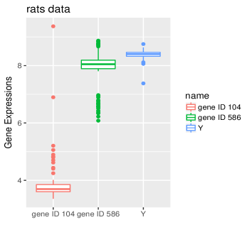
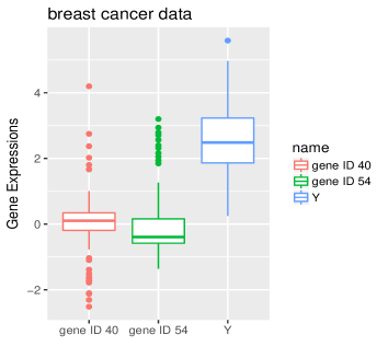
Figure 1: Box-plots for the response and two randomly selected genes for the two datasets. The left panel is for the rats data and the right panel is for the breast cancer data.

We illustrate the CC-SIS and CPC-SIS with the gene expression data on 120 male rats of 12 weeks old, including expression measurements of 31,099 gene probes. It has been analysed in Scheetz et al. (2006) for investigation of the gene regulation in the mammalian and is available at ftp://ftp.ncbi.nlm.nih.gov/geo/series/GSE5nnn/GSE5680/matrix. We follow Ma et al. (2017) and consider the expression of gene TRIM32 (probe 1389163_at) as the response variable $Y$ since it was identified to cause Bardet-Biedl syndrome, closely associated with the human hereditary disease of the retina Chiang et al. (2006). The other gene probes are treated as the covariates ${\bf X}$. We first apply Iglewicz and Hoaglin (1993)’s (IH) approach to check outliers. IH constructs a Z-score $Z_{i}=0.6745(x_{i}-\tilde{x})/\mathrm{MAD}$, where $\mathrm{MAD}$ denotes the median absolute deviation and $\tilde{x}$ stands for the median, and recommends that any $i$ such that $Z_{i}>3.5$ be labeled as outliers. IH method is quite popular in real applications such as engineering. Consequently we find that there are over $60\%$ gene probes having one or more outliers. Figure 1 displays the box-plots for two selected genes and the the response. If one only employs the conventional screening method ignoring the outliers, it would lead to inappropriate results. The copula-based methods may thus be more robust in this situation. In this data analysis, we have the sample $\{(Y_{i},\mathbf{X}_{i}\in\mathbb{R}^{p_{n}}),1\leq i\leq n\}$ with $n=120$ and $p_{n}=31098$.

We report the overlaps of the top $\lfloor n/\log n\rfloor=25$ selected genes by various methods in Table 7. We can see that different methods select quite different genes and such low level of agreement should not be overlooked in practice. Robust and joint screening methods like what we propose in this paper lead to entirely different set of genes which are otherwise screened out by the conventional non-robust and marginal screening approaches. We notice that the CPC-SIS and QPC-SIS have a couple of overlaps, partly because both are conditional screening procedures and able to adjust the confounder effects.

Table 8 gives a summary of top 10 gene probes by different methods along with the p-value resulted from a marginal Wald-test. We then use these 10 genes as regressors and build a joint statistical models to predict $Y$. Linear regression and quantile regression are both considered for this purpose and we display the mean of their prediction errors (PE1 and PE2) over 500 random partitions, where the partition ratio of training sample to test sample is $4:1$ for each partition. The PE is computed as the average of $\{(Y_{i}-\widehat{Y}_{i})^{2},i\in\text{testing set}\}$ and $\widehat{Y}_{i}$ is the predicted value at the $i$th test data point using the model constructed by the training sample with the 10 genes in Table 8. We can see that our proposed copula-based partial correlation screening performs the best with the smallest prediction error. Such a nice prediction result may be attributed to the fact that CPC selects appropriate markers for joint modelling after addressing the distribution heterogeneity and the conditional effects. The heterogeneity problem typically inflates the variance while a purely marginal screener could introduce bias. The prediction error, consists of the variance and the bias components, is thus much smaller after employing the CPC screening method.

5.2.2 Breast Cancer Data

The second data we use to illustrate our proposal is breast cancer data. Breast cancer has become the second most common cancer in the world and the most leading cause in women. There were nearly 1.7 million new cases diagnosed in 2012, according to the worldwide statistics. Meanwhile, approximately 252,710 new cases of invasive breast cancer and 40,610 breast cancer deaths are expected to occur among US women in 2017 as reported in DeSantis et al. (2017). Although major progresses in breast cancer treatment were made, there is also limited ability to predict the metastatic behavior of tumor. Van’t Veer et al. (2002) was the first to study the breast cancer study involving 97 lymph node-negative breast cancer patients 55 years old or younger, of which 46 developed distant metastases within 5 years (metastatic outcome coded as 1) and 51 remained metastases free for at least 5 years (metastatic outcome coded as 0). This expression data set with clinical variables has been well analysed in many papers for classification (Boulesteix et al. (2008), Yu et al. (2012), among others).

In this study, after removing the genes with missing values, there are expression levels of 24,188 gene probes entering into the next analysis. In addition to gene expression measurements, the data for several clinical factors are available as well. Our interest is to identify which gene probes affect the tumor size given other clinical factors $(\mathbf{W})$ including age, histological grade, angioinvasion, lymphocytic infiltration, estrogen receptor and progesterone receiptor status. Therefore, we have the data $\{(Y_{i},\mathbf{X}_{i}\in\mathbb{R}^{p_{n}},\mathbf{W}_{i}\in\mathbb{R}^{r}),1\leq i\leq n\}$ with $n=97$, $p_{n}=24,188$ and $r=6$ for further analysis.

Using the IH method on outlier detection, we find that 18,098 gene probes have at least 1 and at most 29 outliers, suggesting that approximately three quarters of overall gene probes contain extremely large values. The right panel of Figure 1 displays the empirical distribution of the response and two typical covariates. Thus, it is more suitable to apply robust joint screening approach such as the proposed CPC-SIS. We consider the three cases discussed in Section 4 and denote the methods as CPC-SISa₁, CPC-SISa₂ and CPC-SISa₃, respectively). Table 9 gives the overlaps of the selected genes by various methods. A similar conclusion to that in the rats data analysis can be made. Furthermore, Table 10 presents a summary of top 10 gene probes selected by various methods. The results on PE1 and PE2 in Table 10 empirically verifies that our proposed CPC-SIS in Case 3 has the most satisfactory performance in out-of-sample prediction.

6 Conclusion and Discussion

We propose a copula-based correlation and partial correlation to facilitate robust marginal and joint screening for ultrahigh dimensional data sets. Large sample properties for the estimated correlation and sure screening properties for CC and CPC screeners were provided. Empirical studies including simulations and two data applications show that our proposed CC-SIS and CPC-SIS outperform the existing variable screening approaches, when outliers are present in both covariates and response. Therefore, our current proposals are more applicable to the ultrahigh dimensional heterogeneous data. We provide a guideline to carry out variable screening as follows. If the response and predictors are all normal without heteroscedastic variance and the predictors have low correlation, any marginal screening methods (SIS, SIRS, DC-SIS) can be applied. If the response contains outliers or follows a heavy tail distribution and the covariates are normal, robust screening methods (Kendall SIS, QC-SIS, CQC-SIS, CC-SIS) can be employed. If the covariates are highly correlated and conditional variables are available, conditional screening procedures (CSIS, QPC-SIS) can be used. If the data is heteroscedastic for both the response and covariates and the covariates may be highly correlated, then only CPC-SIS can be recommended.

The copula formulation may suggest many possible extensions of our methodology. Firstly, we may consider censored survival time outcome in this framework. See Yue and Li (2018); Hong and Li (2018); Huang et al. (2019) for recent reviews on feature selection and screening for survival analysis. The estimation of copula-based correlation and partial correlation needs to incorporate the random censoring for such data and we need to invoke more complicated empirical process theories to argue the weak convergence results. Secondly, we may even allow the predictors to be censored. See Cheng and Fine (2008) and Cheng and Li (2015) for some earlier discussion. Thirdly, we may consider more pairs of $(\tau,\iota)$ over a candidate set or an interval to incorporate more information on quantile of response and covariates. The relevant theoretical results in this paper can be further generalised. Such extensions to ultrahigh-dimensional data is non-trivial and requires a further development in the future work.

Acknowledgement We thank the Associate Editor and two anonymous referees for constructive comments on our manuscript. This work was partially supported by National Natural Science Foundation of China (Grant No. 11801202), Academic Research Fundings from Ministry of Eduction (MOE) in Singapore: R-155-000-197-112, R-155-000-195-114 and R-155-000-205-114.

Supplementary Materials The supplementary materials consists of two parts: Appendix A and Appendix B. The proofs of all theoretical results stated in the manuscript are given in the Appendix A. Some additional simulations are considered in the Appendix B, which includes the empirical performance of CC and CPC estimators and some discussion on the choice of quantile levels $(\tau,\iota)$ involved in the proposed approaches.

Table 1: Empirical size and power for testing $H_{0}:\varrho_{Y,X_{1}}(\tau,\iota)=\varrho_{Y,X_{2}}(\tau,\iota)$ using CC across $(\tau,\iota)=(0.25,0.25)$, $(0.5,0.5)$ and $(0.75,0.75)$ for Example 1.

			Model (a1)				Model (a2)
$\rho$	Method$(\tau,\iota)$	$n$	$c_{0}=0$	1	2	4	$c_{0}=0$	1	2	4
$0$	CC(0.25,0.25)	200	0.056	0.07	0.07	0.08	0.051	0.48	0.90	1.00
		400	0.051	0.07	0.09	0.08	0.055	0.78	1.00	1.00
	CC(0.5,0.5)	200	0.059	0.33	0.69	0.94	0.057	0.56	0.95	1.00
		400	0.054	0.57	0.93	1.00	0.048	0.85	1.00	1.00
	CC(0.75,0.75)	200	0.057	0.77	0.99	1.00	0.053	0.49	0.90	1.00
		400	0.055	0.96	1.00	1.00	0.050	0.78	1.00	1.00
$0.5$	CC(0.25,0.25)	200	0.055	0.06	0.08	0.14	0.048	0.27	0.62	0.94
		400	0.056	0.06	0.08	0.18	0.052	0.45	0.90	1.00
	CC(0.5,0.5)	200	0.057	0.26	0.56	0.85	0.050	0.29	0.68	0.96
		400	0.053	0.44	0.83	0.98	0.049	0.51	0.93	1.00
	CC(0.75,0.75)	200	0.054	0.71	0.99	1.00	0.052	0.26	0.63	0.93
		400	0.052	0.95	1.00	1.00	0.043	0.47	0.89	1.00
$0.9$	CC(0.25,0.25)	200	0.055	0.08	0.17	0.47	0.048	0.10	0.19	0.43
		400	0.052	0.09	0.29	0.75	0.052	0.14	0.35	0.73
	CC(0.5,0.5)	200	0.061	0.17	0.36	0.63	0.048	0.09	0.20	0.45
		400	0.050	0.27	0.59	0.87	0.048	0.15	0.36	0.75
	CC(0.75,0.75)	200	0.045	0.52	0.91	0.99	0.053	0.09	0.20	0.43
		400	0.047	0.85	1.00	1.00	0.049	0.14	0.36	0.72

Table 2: Empirical size and power for testing $H_{0}:\varrho_{Y,X_{1}|\mathbf{Z}}(\tau,\iota)=\varrho_{Y,X_{2}|\mathbf{Z}}(\tau,\iota)$ using CPC with $(\tau,\iota)=(0.5,0.5)$ in Example 2.

		$\varepsilon\sim N(0,1)$				$\varepsilon\sim\frac{1}{3}Cauchy(0,1)$
$\rho$	$n$	$c_{0}=0$	1	2	4	$c_{0}=0$	1	2	4
$0$	$200$	0.074	0.40	0.84	1.00	0.084	0.45	0.87	1.00
	$400$	0.067	0.65	0.98	1.00	0.073	0.72	0.99	1.00
$0.5$	$200$	0.073	0.40	0.83	1.00	0.081	0.46	0.86	1.00
	$400$	0.066	0.65	0.98	1.00	0.068	0.72	0.99	1.00
$0.9$	$200$	0.077	0.40	0.84	1.00	0.080	0.46	0.86	1.00
	$400$	0.069	0.65	0.98	1.00	0.070	0.72	0.99	1.00

Table 3: Simulation results for Example 3, where MMS stands for the median of the minimum model size and its robust standard deviations (RSD) are given in parenthesis, $\mathcal{P}$ is the proportion of screened sets that cover all active predictors with screening parameter $d_{n}=\lfloor n/\log n\rfloor$.

	$\rho=0.4$				$\rho=0.8$
	$\varepsilon\sim N(0,1)$		$\varepsilon\sim Cauchy(0,1)$		$\varepsilon\sim N(0,1)$		$\varepsilon\sim Cauchy(0,1)$
Method$(\tau,\iota)$	MMS(RSD)	$\mathcal{P}$	MMS(RSD)	$\mathcal{P}$	MMS(RSD)	$\mathcal{P}$	MMS(RSD)	$\mathcal{P}$
Model (b1)
SIS	655 (396)	0.03	790 (227)	0.00	522 (431)	0.12	608 (389)	0.03
SIRS	615 (176)	0.00	669 (158)	0.00	513 (149)	0.00	547 (138)	0.00
DC-SIS	634 (441)	0.09	725 (350)	0.04	460 (527)	0.20	615 (489)	0.13
Kendall-SIS	5 (0)	0.99	5 (1)	0.96	5 (0)	1.00	5 (0)	1.00
CC-SIS(0.25,0.25)	9 (18)	0.80	20 (41)	0.70	5 (0)	1.00	5 (0)	1.00
CC-SIS(0.5,0.5)	6 (7)	0.93	9 (14)	0.84	5 (0)	1.00	5 (0)	1.00
CC-SIS(0.75,0.75)	9 (15)	0.85	14 (40)	0.70	5 (0)	1.00	5 (0)	1.00
QC-SIS(0.25)	710 (315)	0.01	782 (271)	0.00	649 (444)	0.06	678 (406)	0.03
QC-SIS(0.5)	716 (334)	0.01	790 (250)	0.02	665 (438)	0.07	693 (398)	0.06
QC-SIS(0.75)	711 (297)	0.01	751 (314)	0.01	599 (379)	0.04	670 (408)	0.02
CQC-SIS	573 (156)	0.00	614 (149)	0.00	442 (118)	0.00	474 (104)	0.00
Model (b2)
SIS	482 (408)	0.13	638 (376)	0.01	351 (414)	0.15	686 (331)	0.03
SIRS	551 (161)	0.00	589 (195)	0.00	523 (173)	0.00	543 (158)	0.00
DC-SIS	284 (585)	0.30	607 (493)	0.12	230 (569)	0.35	506 (514)	0.17
Kendall-SIS	3 (0)	1.00	3 (0)	1.00	4 (1)	1.00	4 (1)	1.00
CC-SIS(0.25,0.25)	6 (20)	0.78	13 (45)	0.68	5 (2)	0.99	7 (4)	0.94
CC-SIS(0.5,0.5)	3 (1)	0.98	4 (3)	0.95	4 (2)	1.00	5 (1)	1.00
CC-SIS(0.75,0.75)	7 (15)	0.85	14 (43)	0.66	6 (3)	0.99	7 (3)	0.96
QC-SIS(0.25)	615 (356)	0.06	588 (391)	0.05	411 (418)	0.07	598 (411)	0.05
QC-SIS(0.5)	584 (460)	0.07	640 (373)	0.05	539 (474)	0.13	592 (425)	0.10
QC-SIS(0.75)	588 (414)	0.03	579 (353)	0.02	486 (374)	0.09	604 (401)	0.06
CQC-SIS	512 (153)	0.00	562 (155)	0.00	441 (122)	0.00	481 (150)	0.00
Model (b3)
SIS	737 (296)	0.00	768 (204)	0.00	524 (399)	0.01	619 (368)	0.01
SIRS	767 (215)	0.00	745 (182)	0.00	664 (240)	0.00	703 (203)	0.00
DC-SIS	790 (245)	0.00	789 (213)	0.01	722 (276)	0.02	719 (309)	0.01
Kendall-SIS	504 (467)	0.12	475 (442)	0.10	5 (192)	0.65	16 (377)	0.60
CC-SIS(0.25,0.25)	475 (234)	0.02	679 (317)	0.02	252 (365)	0.21	279 (455)	0.14
CC-SIS(0.5,0.5)	483 (357)	0.09	478 (337)	0.07	18 (341)	0.56	53 (357)	0.47
CC-SIS(0.75,0.75)	426 (419)	0.17	281 (460)	0.19	12 (309)	0.59	113 (349)	0.47
QC-SIS(0.25)	791 (199)	0.00	795 (191)	0.00	794 (222)	0.01	781 (225)	0.01
QC-SIS(0.5)	785 (210)	0.00	810 (209)	0.01	750 (266)	0.02	796 (219)	0.04
QC-SIS(0.75)	762 (257)	0.00	793 (240)	0.00	698 (408)	0.01	714 (311)	0.02
CQC-SIS	743 (216)	0.00	749 (177)	0.00	623 (210)	0.00	628 (260)	0.00

Table 4: Simulation results for Example 4 (d1), where $R_{j}$ indicates the median of the rank of the relevant predictors and MMS stands for the median of the minimum model size and its robust standard deviations (RSD) are given in parenthesis.

		$\varepsilon\sim N(0,1)$					$\varepsilon\sim\frac{1}{3}Cauchy(0,1)$
$\rho$	Method$(\tau,\iota)$	$R_{1}$	$R_{2}$	$R_{3}$	$R_{4}$	MMS (RSD)	$R_{1}$	$R_{2}$	$R_{3}$	$R_{4}$	MMS (RSD)
Model (d1)
0.5	SIS	2	2	2	450	450 (235)	3	3	3	411	476 (270)
	SIRS	3	3	3	469	501 (243)	3	3	4	432	466 (258)
	DC-SIS	2	2	2	497	497 (280)	2	2	2	464	464 (220)
	Kendall-SIS	2	2	2	454	454 (228)	2	2	2	467	468 (280)
	CC-SIS(0.25,0.25)	2	2	2	367	372 (331)	2	3	2	382	390 (311)
	CC-SIS(0.5,0.5)	2	2	2	415	425 (272)	2	2	2	396	408 (275)
	CC-SIS(0.75,0.75)	2	2	2	371	387 (324)	2	3	2	378	388 (311)
	QC-SIS(0.25)	2	2	2	478	493 (270)	2	2	2	473	477 (245)
	QC-SIS(0.5)	2	2	2	437	437 (236)	2	2	2	461	463 (331)
	QC-SIS(0.75)	2	2	2	437	438 (227)	2	2	2	408	421 (247)
	QPC-SIS(0.25)	2	2	2	4	4 (0)	2	2	2	4	4 (0)
	QPC-SIS(0.5)	2	2	2	4	4 (0)	2	2	2	4	4 (0)
	QPC-SIS(0.75)	2	2	2	4	4 (0)	2	2	2	4	4 (0)
	CPC-SIS(0.25,0.25)	2	2	2	4	4 (0)	2	2	2	4	4 (0)
	CPC-SIS(0.5,0.5)	2	2	2	4	4 (0)	2	2	2	4	4 (0)
	CPC-SIS(0.75,0.75)	2	2	2	4	4 (0)	2	2	2	4	4 (0)
0.95	SIS	3	3	3	470	498 (306)	214	269	262	466	735 (353)
	SIRS	28	52	45	474	541 (331)	24	26	43	473	584 (376)
	DC-SIS	3	3	3	506	556 (220)	10	12	15	495	610 (240)
	Kendall-SIS	3	3	3	482	529 (296)	3	3	3	486	557 (325)
	CC-SIS(0.25,0.25)	91	95	104	303	481 (276)	88	99	88	318	485 (292)
	CC-SIS(0.5,0.5)	56	49	67	365	499 (383)	53	68	47	354	610 (377)
	CC-SIS(0.75,0.75)	114	92	94	297	470 (301)	125	63	138	318	492 (289)
	QC-SIS(0.25)	3	3	3	470	512 (387)	3	3	3	467	522 (375)
	QC-SIS(0.5)	3	3	3	465	499 (346)	3	3	3	467	506 (382)
	QC-SIS(0.75)	3	3	3	468	520 (379)	3	3	3	469	508 (329)
	QPC-SIS(0.25)	2	2	2	4	4 (0)	2	2	2	4	4 (0)
	QPC-SIS(0.5)	2	2	2	4	4 (0)	2	2	2	4	4 (0)
	QPC-SIS(0.75)	2	2	2	4	4 (0)	2	2	2	4	4 (0)
	CPC-SIS(0.25,0.25)	2	2	2	4	4 (1)	2	2	2	5	5 (1)
	CPC-SIS(0.5,0.5)	2	2	2	4	4 (0)	2	2	2	4	4 (0)
	CPC-SIS(0.75,0.75)	2	2	2	4	4 (1)	2	2	2	4	4 (1)

Table 5: Simulation results for Example 4 (d2), where $R_{j}$ indicates the median of the rank of the relevant predictors and MMS stands for the median of the minimum model size and its robust standard deviations (RSD) are given in parenthesis.

		$\varepsilon\sim N(0,1)$					$\varepsilon\sim\frac{1}{3}Cauchy(0,1)$
$\rho$	Method$(\tau,\iota)$	$R_{1}$	$R_{2}$	$R_{3}$	$R_{4}$	MMS (RSD)	$R_{1}$	$R_{2}$	$R_{3}$	$R_{4}$	MMS (RSD)
Model (d2)
0.5	SIS	2	2	2	530	566 (359)	10	12	14	535	667 (351)
	SIRS	99	93	100	453	485 (304)	107	110	112	478	507 (356)
	DC-SIS	2	2	2	558	629 (393)	2	2	2	554	638 (322)
	Kendall-SIS	2	2	2	514	514 (362)	2	2	2	578	578 (381)
	CC-SIS(0.25,0.25)	3	3	3	437	442 (362)	4	4	4	453	456 (333)
	CC-SIS(0.5,0.5)	3	3	3	339	348 (358)	2	3	3	459	463 (343)
	CC-SIS(0.75,0.75)	3	3	3	440	446 (315)	3	4	5	449	451 (333)
	QC-SIS(0.25)	3	3	3	499	594 (352)	3	3	2	531	618 (363)
	QC-SIS(0.5)	2	2	2	514	583 (377)	2	3	2	501	533 (322)
	QC-SIS(0.75)	3	3	3	532	588 (345)	3	3	3	460	537 (337)
	QPC-SIS(0.25)	3	3	3	2	4 (1)	3	3	3	2	4 (1)
	QPC-SIS(0.5)	2	3	3	2	4 (0)	3	3	3	2	4 (0)
	QPC-SIS(0.75)	3	3	3	2	4 (1)	3	3	3	2	4 (3)
	CPC-SIS(0.25,0.25)	2	2	2	4	4 (2)	2	2	2	4	5 (3)
	CPC-SIS(0.5,0.5)	3	3	3	1	4 (0)	3	3	3	2	4 (0)
	CPC-SIS(0.75,0.75)	2	2	2	4	4 (1)	2	2	3	4	5 (3)
0.95	SIS	182	169	200	557	712 (285)	518	434	435	496	770 (282)
	SIRS	355	388	375	507	729 (290)	450	401	403	507	720 (305)
	DC-SIS	238	191	236	540	762 (335)	347	329	365	507	825 (262)
	Kendall-SIS	192	154	181	534	675 (274)	224	222	196	482	734 (309)
	CC-SIS(0.25,0.25)	266	281	268	443	695 (197)	254	260	255	438	688 (205)
	CC-SIS(0.5,0.5)	292	224	303	473	672 (305)	318	305	213	462	666 (300)
	CC-SIS(0.75,0.75)	262	265	265	441	694 (199)	268	423	284	431	693 (195)
	QC-SIS(0.25)	313	295	338	595	791 (259)	393	394	357	480	755 (280)
	QC-SIS(0.5)	274	304	308	529	795 (283)	291	282	290	480	753 (258)
	QC-SIS(0.75)	259	341	279	529	746 (276)	362	374	376	459	806 (268)
	QPC-SIS(0.25)	112	150	158	4	530 (465)	163	186	162	5	583 (475)
	QPC-SIS(0.5)	106	147	103	3	518 (524)	148	102	96	3	514 (535)
	QPC-SIS(0.75)	148	164	214	3	574 (437)	146	196	126	6	591 (483)
	CPC-SIS(0.25,0.25)	14	11	11	3	270 (478)	13	16	34	6	311 (591)
	CPC-SIS(0.5,0.5)	5	5	6	1	110 (404)	4	4	4	1	24 (371)
	CPC-SIS(0.75,0.75)	11	13	15	3	225 (453)	13	39	14	5	299 (537)

Table 6: Simulation results for Example 5, where $R_{j}$ indicates the median of the rank of the relevant predictors and MMS stands for the median of the minimum model size and its robust standard deviations (RSD) are given in parenthesis.

		$\varepsilon\sim N(0,1)$					$\varepsilon\sim\frac{1}{3}Cauchy(0,1)$
$\rho$	Method$(\tau,\iota)$	$R_{1}$	$R_{2}$	$R_{3}$	$R_{4}$	MMS (RSD)	$R_{1}$	$R_{2}$	$R_{3}$	$R_{4}$	MMS (RSD)
0.5	SIS	12	12	377	4	488 (518)	14	14	396	5	532 (494)
	SIRS	192	215	910	188	910 (96)	236	222	938	193	938 (98)
	DC-SIS	336	305	511	320	744 (162)	305	272	546	324	746 (154)
	Kendall-SIS	2	2	997	1	997 (15)	2	2	998	1	998 (10)
	CC-SIS(0.25,0.25)	3	3	841	2	841 (235)	5	3	830	2	830 (263)
	CC-SIS(0.5,0.5)	3	4	886	2	886 (175)	3	3	895	2	895 (207)
	CC-SIS(0.75,0.75)	3	3	817	2	817 (240)	4	5	865	2	865 (184)
	QC-SIS(0.25)	183	249	713	208	796 (172)	178	148	748	212	806 (170)
	QC-SIS(0.5)	269	241	672	307	823 (160)	232	231	687	296	824 (172)
	QC-SIS(0.75)	223	174	701	259	829 (179)	154	191	731	209	822 (174)
	QPC-SIS(0.25)	6	7	3	3	107 (167)	7	9	3	4	109 (187)
	QPC-SIS(0.5)	4	5	2	3	53 (95)	5	5	3	5	77 (118)
	QPC-SIS(0.75)	5	7	3	3	75 (148)	8	6	3	4	94 (165)
	CPC-SIS(0.25,0.25)	5	4	5	1	28 (58)	7	8	8	2	62 (110)
	CPC-SIS(0.5,0.5)	5	6	1	2	14 (27)	6	6	1	2	19 (34)
	CPC-SIS(0.75,0.75)	5	8	6	1	41 (88)	7	9	7	2	57 (75)
0.95	SIS	5	9	538	4	581 (378)	17	11	525	4	586 (445)
	SIRS	190	231	894	199	894 (95)	246	220	895	186	895 (103)
	DC-SIS	441	303	508	239	771 (171)	189	273	558	348	776 (174)
	Kendall-SIS	2	3	991	1	991 (32)	2	2	990	1	990 (46)
	CC-SIS(0.25,0.25)	3	4	806	2	806 (247)	4	3	825	2	825 (254)
	CC-SIS(0.5,0.5)	3	4	831	2	831 (250)	3	4	836	2	836 (257)
	CC-SIS(0.75,0.75)	3	4	804	2	804 (314)	4	5	758	2	758 (315)
	QC-SIS(0.25)	326	225	624	157	795 (188)	95	202	682	252	805 (192)
	QC-SIS(0.5)	400	244	597	226	804 (189)	135	235	661	318	812 (193)
	QC-SIS(0.75)	312	168	650	143	785 (185)	73	154	695	272	815 (178)
	QPC-SIS(0.25)	5	6	3	3	73 (165)	12	6	3	4	128 (214)
	QPC-SIS(0.5)	4	5	3	3	47 (112)	4	8	3	3	78 (115)
	QPC-SIS(0.75)	5	5	2	3	52 (146)	8	6	3	4	105 (182)
	CPC-SIS(0.25,0.25)	6	5	6	1	31 (47)	6	5	7	2	55 (90)
	CPC-SIS(0.5,0.5)	5	6	1	2	20 (40)	6	5	1	2	18 (42)
	CPC-SIS(0.75,0.75)	6	6	5	1	41 (80)	6	7	7	2	46 (89)

Table 7: The overlaps of selected genes using various approaches for the rats data, where the screening threshold parameter is set as $\lfloor n/\log n\rfloor=25$ for each method and the CPC-SIS applies the algorithm in Case 1.

					QC-SIS$(\tau)$			QPC-SIS$(\tau)$			CC-SIS$(\tau,\iota)$			CPC-SIS$(\tau,\iota)$
	SIS	SIRS	DC-SIS	Kendall-SIS	0.25	0.5	0.75	0.25	0.5	0.75	(0.25,0.25)	(0.5,0.5)	(0.75,0.75)	(0.25,0.25)	(0.5,0.5)	(0.75,0.75)
SIS	25	0	1	3	1	1	0	0	0	0	1	3	3	0	0	0
SIRS	0	25	0	0	0	0	0	0	0	0	0	0	0	0	0	0
DC-SIS	1	0	25	1	2	2	1	0	0	0	0	0	1	0	0	0
Kendall	3	0	1	25	5	12	3	0	0	0	2	5	3	0	0	0
QC-SIS(0.25)	1	0	2	5	25	5	0	0	0	0	3	2	1	0	0	0
QC-SIS(0.5)	1	0	2	12	5	25	3	0	0	0	1	7	1	0	0	0
QC-SIS(0.75)	0	0	1	3	0	3	25	0	0	0	0	1	1	0	0	0
QPC-SIS(0.25)	0	0	0	0	0	0	0	25	3	2	0	0	1	2	1	0
QPC-SIS(0.5)	0	0	0	0	0	0	0	3	25	0	0	0	0	1	1	0
QPC-SIS(0.75)	0	0	0	0	0	0	0	2	0	25	0	0	0	0	1	0
CC-SIS(0.25,0.25)	1	0	0	2	3	1	0	0	0	0	25	1	0	0	0	0
CC-SIS(0.5,0.5)	3	0	0	5	2	7	1	0	0	0	1	25	1	0	0	0
CC-SIS(0.75,0.75)	3	0	1	3	1	1	1	1	0	0	0	1	25	0	0	0
CPC-SIS(0.25,0.25)	0	0	0	0	0	0	0	2	1	0	0	0	0	25	0	0
CPC-SIS(0.5,0.5)	0	0	0	0	0	0	0	1	1	1	0	0	0	0	25	1
CPC-SIS(0.75,0.75)	0	0	0	0	0	0	0	0	0	0	0	0	0	0	1	25

Table 8: Summary of top 10 gene probes selected by different screening methods for the rats data. ID means the selected gene ID and $p$-values are computed as $2(1-\Phi(|\sqrt{n}\widehat{\Omega}_{1}^{-1/2}\widehat{\varrho}_{Y,X}(0.5,0.5)|))$, where $\Phi$ is the cumulative distribution function of standard normal random variable. PE is the mean of prediction errors over 500 random partitions with the partition ratio of training sample to testing sample being $4:1$, where prediction error is defined as the average of $\{(Y_{i}-\widehat{Y}_{i})^{2},i\in\text{testing set}\}$. PE1 and PE2 indicate that $\widehat{Y}_{i}$ is the predicted value via fitting a median regression model and linear model, respectively, using the top 10 genes selected.

	SIS		SIRS		DC-SIS		Kendall-SIS		QC-SIS(0.5)		CC-SIS(0.5,0.5)		QPC-SIS(0.5)		CPC-SIS(0.5, 0.5)
Rank	ID	$p$-value	ID	$p$-value	ID	$p$-value	ID	$p$-value	ID	$p$-value	ID	$p$-value	ID	$p$-value	ID	$p$-value
1	14770	2.1E-05	2828	1.000	146	6.4E-04	6083	8.3E-10	22641	5.2E-11	14726	4.4E-16	18602	0.473	1621	0.469
2	21977	1.8E-05	20503	0.480	260	7.2E-04	5002	4.5E-10	14810	6.4E-12	6889	6.6E-14	4101	0.003	11288	0.001
3	6436	2.0E-08	233	0.152	30768	2.3E-06	14726	4.4E-16	22339	8.0E-13	14701	6.2E-14	12365	0.141	12480	1.000
4	4797	1.7E-08	3962	0.716	30745	1.6E-05	14810	6.4E-12	5002	4.5E-10	20898	7.2E-14	8399	1.000	4398	0.271
5	21150	2.3E-07	7656	0.063	285	1.2E-04	25297	1.5E-11	20898	7.2E-14	22339	8.0E-13	5063	0.026	29604	0.467
6	25573	4.5E-10	20453	0.468	30791	1.6E-07	5259	6.5E-12	31008	1.5E-07	23278	6.2E-13	9223	0.467	22679	1.000
7	12127	9.4E-09	22023	0.047	3849	1.1E-04	5223	2.9E-10	26828	1.8E-08	25117	8.8E-14	21746	0.716	22267	0.065
8	9235	1.6E-07	157	0.208	4626	1.1E-04	31008	1.5E-07	24529	4.2E-10	30548	6.9E-14	14019	0.717	17039	0.148
9	3682	2.5E-06	2575	0.153	4490	2.8E-10	22339	8.0E-13	14414	1.5E-07	4512	8.0E-12	30361	0.277	11796	0.720
10	8670	4.5E-11	2841	0.284	3967	2.1E-07	6021	1.7E-07	20724	2.8E-10	4712	8.4E-12	24759	0.010	20967	0.026
PE1	0.0394		0.0252		0.0290		0.0310		0.0283		0.0330		0.0269		0.0247
PE2	0.0377		0.0269		0.0349		0.0342		0.0344		0.0360		0.0307		0.0257

Table 9: The overlaps of selected genes probes using various approaches for the breast cancer data, where the screening threshold parameter is set as $d_{n}=\lfloor n/\log n\rfloor=21$ for each method. The CPC-SISa₁ means the CPC-SIS in Case 1, the CPC-SISa₂ indicates the CPC-SIS in Case 2 and the CPC-SISa₃ stands for the CPC-SIS in Case 3.

					QC-SIS$(\tau)$			QPC-SIS$(\tau)$			CC-SIS$(\tau,\iota)$			CPC-SISa1	CPC-SISa2	CPC-SISa3
	SIS	SIRS	DC-SIS	Kendall-SIS	0.25	0.5	0.75	0.25	0.5	0.75	(0.25,0.25)	(0.5,0.5)	(0.75,0.75)	(0.5,0.5)	(0.5,0.5)	(0.5,0.5)
SIS	21	8	7	4	1	7	5	1	1	0	2	1	1	0	1	0
SIRS	8	21	13	9	1	15	2	1	0	0	3	5	0	0	1	0
DC-SIS	7	13	21	11	0	8	3	0	0	0	1	6	0	0	1	0
Kendall	4	9	11	21	0	3	4	0	0	0	0	3	0	0	0	0
QC-SIS(0.25)	1	1	0	0	21	1	0	0	0	0	1	0	0	0	0	0
QC-SIS(0.5)	7	15	8	3	1	21	0	1	0	0	3	7	0	0	1	0
QC-SIS(0.75)	5	2	3	4	0	0	21	0	1	0	0	0	5	0	0	0
QPC-SIS(0.25)	1	1	0	0	0	1	0	21	0	0	0	0	0	0	0	0
QPC-SIS(0.5)	1	0	0	0	0	0	1	0	21	0	0	0	0	0	0	0
QPC-SIS(0.75)	0	0	0	0	0	0	0	0	0	21	0	0	0	0	0	0
CC-SIS(0.25,0.25)	2	3	1	0	1	3	0	0	0	0	21	1	0	0	0	0
CC-SIS(0.5,0.5)	1	5	6	3	0	7	0	0	0	0	1	21	0	0	1	0
CC-SIS(0.75,0.75)	1	0	0	0	0	0	5	0	0	0	0	0	21	0	1	0
CPC-SISa1(0.5,0.5)	0	0	0	0	0	0	0	0	0	0	0	0	0	21	0	0
CPC-SISa2(0.5,0.5)	1	1	1	0	0	1	0	0	0	0	0	1	1	0	21	0
CPC-SISa3(0.5,0.5)	0	0	0	0	0	0	0	0	0	0	0	0	0	0	0	21

Table 10: Summary of top 10 gene probes selected by different screening methods for the breast cancer data. ID means the selected gene ID and $p$-values are computed as $2(1-\Phi(|\sqrt{n}\widehat{\Omega}_{1}^{-1/2}\widehat{\varrho}_{Y,X}(0.5,0.5)|))$, where $\Phi$ is the cumulative distribution function of standard normal random variable. PE is the mean of prediction errors over 500 random partitions with the partition ratio of training sample to testing sample being $4:1$, where prediction error is defined as the average of $\{(Y_{i}-\widehat{Y}_{i})^{2},i\in\text{testing set}\}$. PE1 and PE2 indicate that $\widehat{Y}_{i}$ is the predicted value via fitting a median regression model and linear model, respectively, using the top 10 genes selected.

	SIS		SIRS		DC-SIS		Kendall-SIS		QC-SIS(0.5)
Rank	ID	$p$-value	ID	$p$-value	ID	$p$-value	ID	$p$-value	ID	$p$-value
1	24032	3.0E-06	24032	0.000	8349	3.1E-05	17679	6.2E-02	24032	3.0E-06
2	11913	1.2E-07	6841	0.000	24032	3.0E-06	20238	2.3E-02	22705	2.8E-02
3	11870	2.9E-06	9164	0.001	13025	6.7E-04	10408	1.9E-03	6841	6.8E-08
4	17439	6.9E-06	13025	0.001	23670	5.9E-03	1644	6.9E-06	14466	1.8E-03
5	6841	6.8E-08	2172	0.013	20121	1.2E-07	8339	2.6E-03	4767	1.2E-05
6	20938	2.3E-02	17439	0.000	6841	6.8E-08	14028	8.9E-05	5644	2.2E-04
7	10692	2.0E-01	20121	0.000	15674	1.2E-06	23670	5.9E-03	20121	1.2E-07
8	19897	1.5E-03	11870	0.000	1644	6.9E-06	12305	7.3E-04	23670	5.9E-03
9	9164	1.5E-03	22705	0.028	5644	2.2E-04	3929	1.8E-03	13742	1.5E-05
10	17050	2.2E-02	10408	0.002	20238	2.3E-02	14466	1.8E-03	17439	6.9E-06
PE1	1.566		1.483		1.419		1.399		1.409
PE2	1.550		1.398		1.378		1.366		1.367
	CC-SIS(0.5,0.5)		QPC-SIS(0.5)		CPC-SISa1(0.5, 0.5)		CPC-SISa2(0.5, 0.5)		CPC-SISa3(0.5, 0.5)
Rank	ID	$p$-value	ID	$p$-value	ID	$p$-value	ID	$p$-value	ID	$p$-value
1	12801	1.5E-06	11696	0.001	301	0.005	20121	0.000	4132	0.136
2	13742	1.5E-05	672	0.005	18678	0.000	4356	0.001	17568	0.620
3	402	6.2E-05	21944	0.021	3524	0.603	13084	0.008	5459	0.482
4	4862	3.4E-04	6466	0.024	5422	0.021	13191	0.035	1079	0.352
5	8349	3.1E-05	518	0.758	14782	0.023	6436	0.299	23942	0.002
6	9158	1.9E-03	12635	0.022	21431	0.922	10179	0.192	14	0.922
7	12074	6.8E-06	12567	0.609	5239	0.295	20102	0.185	1847	0.169
8	14466	1.8E-03	7160	0.483	777	0.352	1299	0.179	3392	0.505
9	18903	2.5E-02	21188	0.007	20958	0.132	1830	0.381	20369	0.367
10	19774	8.1E-06	11916	0.495	4849	0.460	6025	0.467	390	0.920
PE1	1.404		1.466		1.399		1.436		1.372
PE2	1.290		1.437		1.345		1.304		1.289

References

- Bahadur (1966) Bahadur R.R. (1966). A note on quantiles in large samples. Annals of Mathematical Statistics, 37, 577-580.
- Barut et al. (2016) Barut E., Fan J. and Verhasselt A. (2016). Conditional sure independence screening. Journal of American Statistical Association, 111, 1266-1277.
- Boulesteix et al. (2008) Boulesteix A.L., Porzelius C. and Daumer M. (2008). Microarray-based classification and clinical predictors: on combined classifiers and additional predictive value. Bioinformatics, 24, 1698-1706.
- Chang et al. (2013) Chang J., Tang C.Y. and Wu Y. (2013). Marginal empirical likelihood and sure independence feature screening. Annals of Statistics, 41, 2123-2148.
- Chang et al. (2016) Chang J., Tang C.Y. and Wu Y. (2016). Local independence feature screening for nonparametric and semiparametric models by marginal empirical likelihood. Annals of Statistics, 44, 515-539.
- Cheng and Fine (2008) Cheng Y. and Fine J.P. (2008). Nonparametric estimation of cause-specific cross hazard ratio with bivariate competing risks data. Biometrika, 95, 233-240.
- Cheng and Li (2015) Cheng Y. and Li J. (2015). Time-dependent diagnostic accuracy analysis with censored outcome and censored predictor. Journal of Statistical Planning and Inference, 156, 90-102.
- Cheng et al. (2014) Cheng M., Honda T., Li J. and Peng H. (2014) Nonparametric independence screening and structure identification for ultra-high dimensional longitudinal data. Annals of Statistics, 42, 1819-1849.
- Chiang et al. (2006) Chiang A.P., Beck J.S., Yan H.J., et al. (2006). Homozygosity mapping with SNP arrays identifies TRIM32, an E3 ubiquitin ligase, as a Bardet Biedl syndrome gene (BBS11). Proceedings of the National Academy of Sciences, 103, 6287-6292.
- Chu et al. (2016) Chu W., Li R. and Reimherr M. (2016). Feature screening for time-varying coefficient models with ultrahigh dimensional longitudinal data. Annals of Applied Statistics, 10, 596-617.
- DeSantis et al. (2017) DeSantis C.E., Ma J., Sauer A.G., Newman L. A. and Jemal A. (2017). Breast cancer statistics, 2017, racial disparity in mortality by state. CA: A Cancer Journal for Clinicians, 67, 439-448. Harvard
- Fan and Lv (2008) Fan J. and Lv J. (2008). Sure independence screening for ultrahigh dimensional feature space. Journal of the Royal Statistical Society, Series B, 70, 849-911.
- Fan et al. (2011) Fan J., Feng Y. and Song R. (2011). Nonparametric independence screening in sparse ultra-high-dimensional additive models. Journal of the American Statistical Association, 106, 544-557.
- Fan et al. (2014) Fan J., Ma Y., Dai W. (2014) Nonparametric independent screening in sparse ultra-high dimensional varying coefficient models. Journal of the American Statistical Association, 109, 1270-1284.
- Fan and Song (2010) Fan J. and Song R. (2010). Sure independence screening in generalized linear models with NP-dimensionality. Annals of Statistics, 38, 3567-3604.
- He et al. (2013) He X., Wang, L. and Hong H. (2013). Quantile-adaptive model-free variable screening for high-dimensional heterogeneous data. Annals of Statistics, 41, 342-369.
- Huang et al. (2019) Huang, T., McKeague, I., Qian, M. (2018). Marginal screening for high-dimensional predictors of survival outcomes. Statistica Sinica, in press.
- Hong and Li (2018) Hong, H. and Li Y. (2018). Feature selection of ultrahigh-dimensional covariates with survival outcomes: a selective review. Applied Mathematics-A Journal of Chinese Universities, 32: 379-396.
- Iglewicz and Hoaglin (1993) Iglewicz B. and Hoaglin D. (1993), Volume 16: How to detect and handle outliers, The ASQC Basic References in Quality Control: Statistical Techniques, Edward F. Mykytka, Ph.D., Editor.
- Koenker (2005) Koenker R. (2005). Quantile Regression, New York: Cambridge University Press.
- Li et al. (2015) Li G., Li Y. and Tsai C.L. (2015). Quantile correlations and quantile autoregressive modeling. Journal of the American Statistical Association, 110, 246-261.
- Li et al. (2012a) Li G., Peng H., Zhang J. and Zhu L. (2012). Robust rank correlation based screening. Annals of Statistics, 40, 1846-1877.
- Li et al. (2016) Li J., Zheng Q., Peng L. and Huang Z. (2016). Survival impact index and ultrahigh-dimensional model-free screening with survival outcomes. Biometrics, 72, 1145-1154.
- Li et al. (2012b) Li R., Zhong W. and Zhu L. (2012). Feature screening via distance correlation learning. Journal of the American Statistical Association, 107, 1129-1139.
- Liu et al. (2014) Liu J., Li R. and Wu R. (2014). Feature selection for varying coefficient models with ultrahigh-dimensional covariates. Journal of the American Statistical Association, 109, 266-274.
- Ma and Zhang (2016) Ma X. and Zhang J. (2016). Robust model-free feature screening via quantile correlation. Journal of Multivariate Analysis, 143, 472-480.
- Ma et al. (2017) Ma S., Li R. and Tsai C. (2017). Variable screening via quantile partial correlation. Journal of the American Statistical Association, 112, 650-663.
- Nadaraya (1964) Nadaraya E. A. (1964). On estimating regression. Theory of Probability and Its Applications, 9, 141-142.
- Nelsen (2007) Nelsen R. B. (2007). An Introduction to Copulas. Springer Science & Business Media.
- Scheetz et al. (2006) Scheetz T. E., Kim K.Y. A., Swiderski R. E., et al.(2006). Regulation of gene expression in the mammalian eye and its relevance to eye disease. Proceedings of the National Academy of Sciences of the United States of America, 103, 14429-14434.
- Song et al. (2014) Song R., Lu W., Ma S. and Jeng X.J. (2014). Censored rank independence screening for high-dimensional survival data. Biometrika, 101, 799-814.
- Van’t Veer et al. (2002) Vant Veer L.J., Dai H., van de Vijver M.J., et al. (2002). Gene expression profiling predicts clinical outcome of breast cancer. Nature, 415, 530-536.
- Watson (1964) Watson G. S. (1964). Smooth regression analysis. Sankhya: The Indian Journal of Statistics, Series A, 26, 359-372.
- Wu and Yin (2015) Wu Y. and Yin G. (2015). Conditional qunatile screening in ultrahigh-dimensional heterogeneous data. Biometrika, 102, 65-76.
- Xia et al. (2018) Xia X., Li J. and Fu B. (2018). Conditional quantile correlation learning for ultrahigh dimensional varying coefficient models and its application in survival analysis. Statistica Sinica, Accepted.
- Xia et al. (2016a) Xia X., Jiang B., Li J. and Zhang W. (2016). Low-dimensional Confounder Adjustment and High-dimensional Penalized Estimation for Survival Analysis. Lifetime Data Analysis, 22(4), 547-569.
- Xia et al. (2016b) Xia X., Yang H., and Li J. (2016). Feature screening for generalized varying coefficient models with application to dichotomous responses. Computational Statistics and Data Analysis. 102, 85-97.
- Yu et al. (2012) Yu T., Li J. and Ma S. (2012). Adjusting confounders in ranking biomarkers: a model-based ROC approach. Briefings in Bioinformatics, 13, 513-523.
- Yue and Li (2018) Yue M. and Li J. (2018). Improvement Screening for Ultra-High Dimensional Data with Censored Survival Outcomes and Varying Coefficients. International Journal of Biostatistics. 13(1): 16.
- Zhao and Li (2012) Zhao D.S. and Li Y. (2012). Principled sure independence screening for Cox models with ultra-high-dimensional covariates. Journal of Multivariate Analysis, 105, 397-411.
- Zhu et al. (2011) Zhu L., Li L., Li R. and Zhu L.X. (2011). Model-Free feature screening for ultrahigh dimensional data. Journal of the American Statistical Association, 106, 1464-1475.