Decays $A\to Z\gamma\gamma$ and $\phi\to Z\gamma\gamma$ ($\phi=h,H$) in two-Higgs doublet models

Abstract

The one-loop contributions to the decays of the $CP$-odd and $CP$-even scalar bosons $A\to Z\gamma\gamma$ and $\phi\to Z\gamma\gamma$ ($\phi=h,H$) are calculated within the framework of $CP$-conserving THDMs, where they are induced by box and reducible Feynman diagrams. The behavior of the corresponding branching ratios are then analyzed within the type-II THDM in a region of the parameter space around the alignment limit and still consistent with experimental data. It is found that the $A\to Z\gamma\gamma$ branching ratio is only relevant when $m_{A}>m_{H}+m_{Z}$, but it is negligible otherwise. For $m_{A}>600$ GeV and $t_{\beta}\simeq O(1)$, $BR(A\to Z\gamma\gamma)$ can reach values of the order of $10^{-5}-10^{-4}$, but it decreases by about one order of magnitude as $t_{\beta}$ increases up to 10. A similar behavior is followed by the $H\to Z\gamma\gamma$ decay, which only has a non-negligible branching ratio when $m_{H}>m_{A}+m_{Z}$ and can reach the level of $10^{-4}-10^{-3}$ for $m_{H}>600$ GeV and $t_{\beta}\simeq O(1)$. We also estimated the branching ratios of these rare decays in the type-I THDM, where they can be about one order of magnitude larger than in type-II THDM. As far as the $h\to Z\gamma\gamma$ decay is concerned, since the properties of this scalar boson must be nearly identical to those of the SM Higgs boson, the $h\to Z\gamma\gamma$ branching ratio does not deviates significantly from the SM prediction, where it is negligibly small, of the order of $10^{-9}$. This result is in agreement with previous calculations.

I Introduction

The standard model (SM) has provided a successful description of the observed electroweak phenomena at the energy scales explored until now, as confirmed recently with the discovery of the Higgs boson by the ATLAS and CMS experiments at the CERN LHC Aad et al. (2012); Chatrchyan et al. (2012). Nonetheless, it is worth to explore whether there is a unique Higgs boson, as predicted by the SM, or the electroweak symmetry breaking (EWSB) mechanism requires additional Higgs bosons. To address some SM flaws, a plethora of extension models have been proposed, several of which contain a scalar sector with more than one Higgs multiplet, thereby predicting more than one physical Higgs boson. If experimental data reveal the existence of any additional Higgs bosons, it will be crucial to test what extension model is consistent with such particles. The simplest of such theories are two-Higgs doublet models (THDMs) Gunion et al. (2000); Branco et al. (2012), which are obtained by adding a second complex $SU(2)_{L}$ Higgs doublet to the SM one. These models respect the $\rho=1$ relation at the tree-level, contrary to other higher-dimensional Higgs-multiplet models. Also, in spite of its simplicity, THDMs can predict several new phenomena absent in the SM, such as new sources of $CP$ violation, tree-level scalar-mediated flavor changing neutral currents (FCNCs), a dark matter candidate, etc. After EWSB, three of the eight degrees of freedom are removed from the spectrum to provide the longitudinal modes of the $W^{\pm}$ and $Z$ gauge bosons. Five physical Higgs bosons remain as remnant: a charged Higgs boson pair $H^{\pm}$ and three neutral Higgs bosons $h$, $H$, and $A$. If the scalar sector respects $CP$ invariance, the neutral scalar bosons are $CP$-eigenstates: $h$ and $H$ are $CP$-even, whereas $A$ is $CP$-odd. It is usually assumed that one of the neutral $CP$-even scalar bosons is the one observed at the LHC. The most general $CP$-conserving THDMs have tree-level FCNCs Atwood et al. (1997), which can be removed by imposing a $Z_{2}$ discrete symmetry that forbids such interactions at the tree-level Glashow and Weinberg (1977). In this scenario, there are four THDM types, which are typically known as type-I, type-II, lepton-specific Cao et al. (2009) and flipped THDM Aoki et al. (2009). It turns out that type-II THDM is the most studied in the literature as it has the same Yukawa couplings as the minimal supersymmetric standard model (MSSM), therefore its still-allowed region of parameter space has been considerably studied.

Since the proposal of the Higgs mechanism, the phenomenology of the Higgs bosons has been the focus of considerable attention. As for the dominant tree-level decay modes of a $CP$-even Higgs boson $h\to\bar{f}f$ and $h\to VV$ ($V=W,Z$), they have been long studied in the literature both in the SM and several of its extensions, along with the one-loop induced decays $h\to\gamma\gamma$, $h\to\gamma Z$, and $h\to gg$. Although the $h\to\gamma\gamma$ decay has a tiny branching ratio for a $125$ GeV Higgs boson, it was very helpful for the detection of the SM Higgs boson. This decay mode has the advantage of a relatively low background, so it was fundamental in the design of the ATLAS and CMS detectors. As for the $h\to gg$ decay, it is undetectable but it is fundamental to compute the cross section for Higgs production via gluon fusion.

It is expected that the data collected at the LHC may allow us to search for any other rare decays of the Higgs boson Kling et al. (2016), such as lepton flavor changing Higgs decays $h\to\bar{\ell}_{i}\ell_{j}$ ($i\neq j$) or invisible Higgs decays $h\to\cancel{E}_{T}$, which are forbidden in the SM and can shed light on any new physics effect. Even more, with the prospect of a future Higgs boson factory, other exotic decays of the Higgs boson could be at the reach of experimental detection. In particular, the rare decay $h\to Z\gamma\gamma$ is very suppressed in the SM as it arises at the one-loop level via the exchange of charged particles, so it can offer a relatively clean signal of new physics: two energetic photons plus a back to back lepton anti-lepton pair. This process can also provide a test for the couplings of the Higgs boson to the particles running into the loops, which can be SM particles or any new charged particle predicted by other extension models. A similar decay is $h\to Zgg$, which at the leading order can be straightforwardly calculated from the $h\to Z\gamma\gamma$ one. In addition, the study of the $hZ\gamma\gamma$ and $hZgg$ vertices would allow us to obtain the leading order contributions to the cross section of $hZ$ pair production via photon fusion $\gamma\gamma\to hZ$ and gluon fusion $gg\to hZ$ Kniehl (1990a); Gounaris et al. (2001).

On the other hand, a $CP$-odd scalar boson has fewer decay channels and so it is worth studying some one-loop induced decays of such a particle. At tree level, its dominant decay channels are $A\to\bar{f}f$, $A\to Zh(H)$ and $A\to W^{\pm}H^{\mp}$, when kinematically allowed, whereas at the one-loop level a $CP$-odd scalar boson can decay as $A\to gg$, $A\to\gamma\gamma$ and $A\to Z\gamma$ Gunion et al. (2000). These decay channels can have significant branching ratios in some regions of the parameter space. Other one-loop induced decay modes such as $A\to WW$ and $A\to ZZ$ have already been studied in Mendez and Pomarol (1991); Diaz-Cruz et al. (2014), though they are more suppressed than the aforementioned decay channels.

In this work we are interested in studying the $A\to Z\gamma\gamma$ and $\phi\to Z\gamma\gamma$ ($\phi=h,H$) decay modes in the context of THDMs, which induce these processes at the one-loop level via box and reducible Feynman diagrams, with contributions from charged fermions, mainly from the top and bottom quarks. The $W$ gauge boson and the charged scalar boson $H^{\pm}$ can only contribute through reducible diagrams to the $A\to Z\gamma\gamma$ decay . The respective decay of the SM Higgs boson has already been studied: the decay $h\to Z\gamma\gamma$ was studied in Ref. Abbasabadi and Repko (2005) and the analogue decay $h\to Zgg$ was studied in Kniehl (1990b); Abbasabadi and Repko (2008). To our knowledge, the $A\to Z\gamma\gamma$ decay has not been studied until now.

The organization of this paper is as follows. Section II is devoted to a brief discussion of the general THDM, focusing on the $CP$-conserving THDMs. In Sec. III we present the details of the calculation of the decays $A\to Z\gamma\gamma$ and $\phi\to Z\gamma\gamma$ ($\phi=h,H$) by the Passarino-Veltman reduction scheme. We present the analytical expressions for the invariant amplitudes, the decay widths, as well as the kinematic distributions of the invariant mass of the photons and the energy of the $Z$ gauge boson, which can be useful to disentangle the decay signal from its potential background. The numerical analysis of the branching ratios within type-II THDM is presented in Sec. IV, whereas the conclusions and outlook are presented in Sec. V. The Feynman rules necessary for the calculations and some lengthy formulas are presented in the appendices.

II Two-Higgs doublet models

THDMs have been largely studied in the literature Gunion et al. (2000). We will present here a brief outline of $CP$-conserving THDMs, including only those details relevant for our calculation. For the interested reader, a comprehensive review of these models can be found in Branco et al. (2012).

II.1 THDM Lagrangian

In THDMs, two complex $SU(2)_{L}$ Higgs doublets $\Phi_{i}$ are introduced in the scalar sector:

$$\Phi_{i}=\left(\begin{array}[]{c}\phi_{i}^{+}\\ {\dfrac{v_{i}+\phi_{i}^{0}+i\phi_{i}}{\sqrt{2}}}\end{array}\right)\;\;\;(i=1,2),$$ (1)

where $v_{i}$ are the vacuum expectation values (VEVs) of the neutral components, which satisfy $v_{1}^{2}+v_{2}^{2}=v^{2}$, with $v=246$ GeV. A well known parameter of this model is the VEVs ratio $\tan\beta\equiv t_{\beta}=v_{2}/v_{1}$. The EWSB mechanism is achieved by the most general $SU(2)_{L}\times U(1)_{Y}$ gauge invariant Lagrangian

$$\mathcal{L}=\sum_{i}|D_{\mu}\Phi_{i}|^{2}-V(\Phi_{1},\Phi_{2})+\mathcal{L}_{Yuk}+\mathcal{L}_{SM},$$ (2)

where $|D_{\mu}\Phi_{i}|^{2}$ is the kinetic term for the two-Higgs doublets, with $D_{\mu}$ the SM covariant derivative, $V(\Phi_{1},\Phi_{2})$ is the Higgs potential, $\mathcal{L}_{Yuk}$ denotes the Yukawa interactions between $\Phi_{i}$ and the SM fermions, and $\mathcal{L}_{SM}$ describes the $SU(2)_{L}\times U(1)_{Y}$ interactions of fermions and gauge bosons.

The most general gauge-invariant renormalizable potential $V(\Phi_{1},\Phi_{2})$ for THDMs is a hermitian combination of electroweak invariant combinations. It contains 14 parameters and can give rise to new sources of $CP$ violation Ginzburg and Krawczyk (2005). However, as long as $CP$ is conserved in the Higgs sector, the scalar potential for the two doublets $\Phi_{1}$ and $\Phi_{2}$ with hypercharge $+1$ can be written in terms of 8 parameters as follows Gunion et al. (2000); Branco et al. (2012)

$$\begin{split}V(\Phi_{1},\Phi_{2})&=m_{11}^{2}\Phi_{1}^{\dagger}\Phi_{1}+m_{22}^{2}\Phi_{2}^{\dagger}\Phi_{2}-m_{12}^{2}(\Phi_{1}^{\dagger}\Phi_{2}+\mbox{h.c.})+\dfrac{\lambda_{1}}{2}(\Phi_{1}^{\dagger}\Phi_{1})^{2}+\dfrac{\lambda_{2}}{2}(\Phi_{2}^{\dagger}\Phi_{2})^{2}\\ &+\lambda_{3}(\Phi_{1}^{\dagger}\Phi_{1})(\Phi_{2}^{\dagger}\Phi_{2})+\lambda_{4}(\Phi_{1}^{\dagger}\Phi_{2})(\Phi_{2}^{\dagger}\Phi_{1})+\dfrac{\lambda_{5}}{2}\Bigl{[}(\Phi_{1}^{\dagger}\Phi_{2})^{2}+\mbox{h.c.}\Bigr{]}\end{split}$$ (3)

After EWSB, three of the eight degrees of freedom of the two Higgs doublets are the Goldstone bosons $(G^{\pm},\xi)$, which are absorbed as longitudinal components of the $W^{\pm}$ and $Z$ gauge bosons, whereas the remaining five degrees of freedom become the physical Higgs bosons: there is a pair of charged scalar bosons $H^{\pm}$, two neutral $CP$-even scalar bosons $h$ and $H$, where $m_{h}<m_{H}$ by convention, and one neutral $CP$-odd scalar $A$. Since all the parameters appearing in the potential are real, there are no bilinear mixing terms, which is why the neutral mass eigenstates are also $CP$ eigenstates. In the neutral sector the following mass term appears

$$\mathcal{L}_{\mbox{mass}}^{A}=(\phi_{1}\;,\;\phi_{2})V_{A}^{2}\left(\begin{array}[]{c}\phi_{1}\\ \phi_{2}\end{array}\right),$$ (4)

with

$$V_{A}^{2}=\dfrac{1}{2}\left(\frac{m_{12}^{2}}{v_{1}v_{2}}-\lambda_{5}\right)\left(\begin{array}[]{cc}\;\;v_{2}^{2}&-v_{1}v_{2}\\ -v_{1}v_{2}&\;\;v_{1}^{2}\end{array}\right).$$ (5)

Once $V_{A}^{2}$ is diagonalized, one obtains the neutral Goldstone boson $\xi$ and the physical $CP$-odd Higgs boson via the rotation

$$\left(\begin{array}[]{c}\xi\\ A\end{array}\right)=\left(\begin{array}[]{rc}\cos\beta&\sin\beta\\ -\sin\beta&\cos\beta\end{array}\right)\left(\begin{array}[]{c}\phi_{1}\\ \phi_{2}\end{array}\right),$$ (6)

with $m_{A}^{2}=\left(\dfrac{m_{12}^{2}}{v_{1}v_{2}}-\lambda_{5}\right)v^{2}$.

In the case of the $CP$-even scalar bosons we have

$$\mathcal{L}_{\mbox{mass}}^{H}=\dfrac{1}{2}(\phi_{1}^{0}\;\;\phi_{2}^{0})V_{H}^{2}\left(\begin{array}[]{c}\phi_{1}^{0}\\ {\phi_{2}^{0}}\end{array}\right),$$ (7)

where

$$V_{H}^{2}=\left(\begin{array}[]{cc}A_{s}&B_{s}\\ B_{s}&C_{s}\end{array}\right),$$ (8)

with $A_{s}=\lambda_{1}v_{1}^{2}+\dfrac{v_{2}}{v_{1}}m_{12}^{2}$, $B_{s}=m_{12}^{2}-\dfrac{v_{1}}{v_{2}}(v_{1}^{2}\lambda_{1}-2m_{11}^{2})$, and $C_{s}=\lambda_{2}v_{2}^{2}+\dfrac{v_{1}}{v_{2}}m_{12}^{2}$. The physical $CP$-even Higgs bosons with masses $m_{H}$ y $m_{h}$ are obtained by rotating the original basis by an angle $\alpha$

$$\left(\begin{array}[]{c}H\\ h\end{array}\right)=\left(\begin{array}[]{rc}\cos\alpha&\sin\alpha\\ -\sin\alpha&\cos\alpha\end{array}\right)\left(\begin{array}[]{c}\phi_{1}^{0}\\ {\phi_{2}^{0}}\end{array}\right),$$ (9)

with $m_{H,h}^{2}=\dfrac{1}{2}\left((A_{s}+C_{s})\pm\sqrt{(A_{s}-C_{s})^{2}+B_{s}^{2}}\right)$ and the mixing angle given as

$$\sin 2\alpha=\frac{2B_{s}}{\sqrt{(A_{s}-C_{s})^{2}+4B_{s}^{2}}}.$$ (10)

II.2 Flavor-conserving THDMs

As far as the Yukawa Lagrangian $\mathcal{L}_{Yuk}$ is concerned, the scalar-to-fermion couplings are not univocally determined by the gauge structure of the model. The most general Yukawa Lagrangian for THDMs is Branco et al. (2012)

$$-\mathcal{L}_{Yuk}=\sum_{k=1}^{2}\left[\bar{L}_{L}\Phi_{k}Y^{\ell}_{k}\ell_{R}+\bar{Q}_{L}\left(\Phi_{k}Y^{d}_{k}d_{R}+\tilde{\Phi}_{k}Y^{u}_{k}u_{R}\right)\right]+{\rm H.c.},$$ (11)

where $\tilde{\Phi}_{j}=i\tau_{2}\Phi_{j}$, $Y^{f}$ are $3\times 3$ complex matrices, and the left- and right-handed fermion fields are tree-vectors in flavor space.

To prevent tree-level FCNCs it is usual to introduce a discrete $Z_{2}$ symmetry respected by the $\Phi_{i}$ doublets and the fermions. Under this symmetry one of the scalar doublets is even $\Phi_{2}\rightarrow\Phi_{2}$ and the other one is odd $\Phi_{1}\rightarrow-\Phi_{1}$. This gives rise to four types of THDMs, which are usually known as type-I THDM, type-II THDM, lepton-specific THDM and flipped THDM. The way in which each Higgs doublet couples to the fermions in these models is summarized in Table 1. On the other hand, if no $Z_{2}$ discrete symmetry is imposed, there will be tree-level FCNCs. In such a scenario both doublets couple to the charged leptons and quarks. This model is known as type-III THDM Cheng and Sher (1987); Braeuninger (2010). In this work, however, we are not interested in this realization of THDMs.

Table 1: Couplings of quarks and leptons to the Higgs doublets $\Phi_{i}$ in THDMs with natural flavor conservation. The superscript $i$ stands for the generation index. There is another version of THDMs, known as type-III THDM, in which both Higgs doublets couple to the leptons and quarks simultaneously, thereby giving rise to tree-level FCNCs Gunion et al. (2000); Branco et al. (2012).

THDM	$u^{i}$	$d^{i}$	$e^{i}$
type-I	$\Phi_{2}$	$\Phi_{2}$	$\Phi_{2}$
type-II	$\Phi_{2}$	$\Phi_{1}$	$\Phi_{1}$
lepton-specific	$\Phi_{2}$	$\Phi_{2}$	$\Phi_{1}$
flipped	$\Phi_{2}$	$\Phi_{1}$	$\Phi_{2}$

Although we will present a rather general calculation within flavor-conserving THDMs, the numerical analysis will be carried out in the context of the type-II THDM, which is by far the most studied THDM since it shares the same Yukawa interactions as the MSSM. The most distinctive difference between the type-II THDM and the MSSM is that the former does not have a strict upper bound on the mass of the lightest Higgs boson, which is an important feature of the latter. In addition, in THDMs the scalar boson self couplings are arbitrary and so is the mixing parameter $\alpha$, which in the MSSM is given in terms of $\tan\beta$ and the scalar boson masses.

Our calculation is to be performed in the unitary gauge. The Feynman rules for THDMs can be obtained once the Lagrangian is expanded in terms of mass eigenstantes and can be found for instance in Refs. Branco et al. (2012); Gunion et al. (2000). We present those Feynman rules required by our calculation in Appendix A.

III $A\to Z\gamma\gamma$ and $\phi\to Z\gamma\gamma$ ($\phi=h,H,$) decay widths

III.1 Kinematic conditions

We now turn to present the $A\to Z\gamma\gamma$ and $\phi\to Z\gamma\gamma$ ($\phi=h,H,$) decay widths. We first present the kinematics conditions, which are defined according to the following notation for the external 4-momenta

$$\phi(p)\to\gamma_{\mu}(k_{1})+\gamma_{\nu}(k_{2})+Z_{\alpha}(k_{3}).$$ (12)

The mass-shell conditions thus read $p^{2}=m_{\phi}^{2}$, $k_{3}^{2}=m_{Z}^{2}$ and $k_{1}^{2}=k_{2}^{2}=0$. We now introduce the following Lorentz invariant quantities:

$$s_{1} =(k_{1}+k_{3})^{2},$$ (13)

$$s_{2} =(k_{2}+k_{3})^{2},$$ (14)

$$s =(k_{1}+k_{2})^{2}.$$ (15)

These variables are not all independent as $s_{1}+s_{2}+s=m_{\phi}^{2}+m_{Z}^{2}$ by four-momentum conservation. In our calculation, we express all the scalar products between the four-momenta $k_{1}$, $k_{2}$ and $k_{3}$ in terms of the Lorentz invariant variables $s_{1}$, $s_{2}$ and $s$ as well as the scaled variable $\mu_{Z}=m_{Z}^{2}/m_{\phi}^{2}$.

In addition, because of the transversality conditions obeyed by the gauge bosons, i.e., $k_{1}\cdot\epsilon^{\mu}(k_{1})=k_{2}\cdot\epsilon^{\nu}(k_{2})=k_{3}\cdot\epsilon^{\alpha}(k_{3})=0$, we drop from the invariant amplitudes any terms proportional to $k_{1}^{\mu}$, $k_{2}^{\nu}$, and $k_{3}^{\alpha}$.

All the above kinematic conditions probe useful to simplify the calculation. We now present the invariant amplitudes for the $A\to Z\gamma\gamma$ and $\phi\to Z\gamma\gamma$ ($\phi=h,H$) decays, which are induced at the one-loop level at the lowest order in perturbation theory.

III.2 $A\to Z\gamma\gamma$ decay invariant amplitude

There are two sets of Feynman diagrams that induce this decay: box diagrams and reducible diagrams. Once the invariant amplitude for each Feynman diagram was written down in the unitary gauge, we used the Passarino-Veltman reduction scheme to solve the loop integrals Passarino and Veltman (1979), which were reduced down to a combination of two-, three- and four-point scalar functions. The algebra was carried out with the aid of the Mathematica package FeynCalc Mertig et al. (1991). We first present the invariant amplitude arising from the box diagrams.

III.2.1 Box diagram contribution

In Fig. 1 we show the box diagrams that contribute to the $A\to Z\gamma\gamma$ decay. The dynamical content is rather simple in the sense that there is only one kind of particles circulating into the loop, namely, SM charged fermions. Other charged particles do not contribute to this decay at the one-loop level in THDMs: due to $CP$ invariance in the scalar sector, the $CP$-odd scalar $A$ does not couple to a pair of $W$ gauge bosons or charged scalars $H^{\mp}$, though it can couple to a $W^{\pm}H^{\mp}$ pair. However, the $VW^{\mp}H^{\pm}$ vertex ($V=\gamma,Z$) is absent at the tree-level and so the $A\to Z\gamma\gamma$ decay cannot proceed via box diagrams with both $W^{\mp}$ and $H^{\mp}$ particles. The main contributions of box diagrams are thus expected to arise from the heaviest fermions. For small $t_{\beta}$, the top quark contribution would dominate, whereas for large $t_{\beta}$ the bottom quark contribution would become relevant. This is due to the presence of the factors $1/t_{\beta}$ and $t_{\beta}$ appearing in the Yukawa couplings for the top and bottom quarks, respectively, as will be shown below.

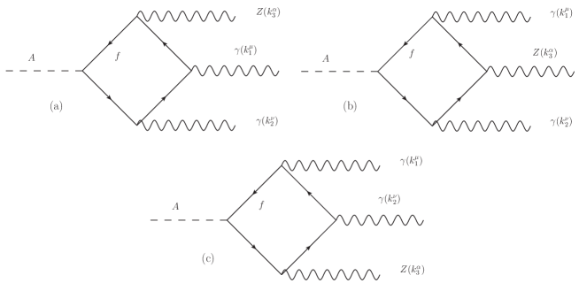
Figure 1: Box diagrams that contribute to the $A\to Z\gamma\gamma$ decay in the THDM. There are three additional diagrams that are obtained by exchanging the photons. Similar diagrams also contribute to the $\phi\to Z\gamma\gamma$ ($\phi=h,H$) decay, after the replacement $A\to\phi$.

Once the Passarino-Veltman reduction scheme was applied, we performed several test on our results. First, we verified that the invariant amplitude for all the box diagrams is gauge invariant under $U(1)_{\mbox{em}}$, i.e. it vanishes when the photon four-momenta are replaced by their polarization vectors. We also verified that Bose symmetry is respected and that ultraviolet divergences cancel out. The invariant amplitude for the $A\to Z\gamma\gamma$ decay can be cast in the following gauge-invariant manifest form

$$\mathcal{M}(A\to Z\gamma\gamma)=\mathcal{M}^{\alpha\mu\nu}(A\to Z\gamma\gamma)\;\epsilon_{\alpha}^{*}(k_{3})\epsilon_{\mu}^{*}(k_{1})\epsilon_{\nu}^{*}(k_{2}),$$ (16)

with the Lorentz structures given as follows

$$\begin{split}\mathcal{M}^{\alpha\mu\nu}(A\to Z\gamma\gamma)&=\mathcal{F}_{1}\;k_{1}^{\alpha}\Bigl{(}k_{1}^{\nu}k_{2}^{\mu}-k_{1}\cdot k_{2}\;g^{\mu\nu}\Bigr{)}+\mathcal{F}_{2}\Bigl{(}k_{3}^{\nu}(k_{1}^{\alpha}k_{2}^{\mu}-k_{1}\cdot k_{2}\;g^{\alpha\mu})+k_{2}\cdot k_{3}(k_{1}^{\nu}g^{\alpha\mu}-k_{1}^{\alpha}g^{\mu\nu})\Bigr{)}\\ &+\frac{\mathcal{F}_{3}}{m_{A}^{2}}\;k_{2}^{\alpha}\Bigl{(}k_{3}^{\mu}(k_{2}\cdot k_{3}\;k_{1}^{\nu}-k_{1}\cdot k_{2}\;k^{\nu})+k_{1}\cdot k(k_{3}^{\nu}k_{2}^{\mu}-k_{2}\cdot k_{3}\;g^{\mu\nu})\Bigr{)}+\Bigl{(}k_{1}^{\mu}\leftrightarrow k_{2}^{\nu}\Bigr{)},\end{split}$$ (17)

where the form factors $\mathcal{F}_{i}$ depend on $s_{1}$, $s_{2}$, $s$, and $\mu_{Z}$, though we will refrain from writing out such a dependency explicitly. These form factors will receive contributions from both box and reducible diagrams, which means that the latter will not generate additional Lorentz structures. We can thus write $\mathcal{F}_{i}=\mathcal{F}_{i}^{Box}+\mathcal{F}_{i}^{RD}$, where the notation is self-explanatory. The expressions for the box diagram contributions are too lengthy and they are presented in Appendix B in terms of Passarino-Veltman scalar functions.

III.2.2 Reducible diagram contribution

There are also reducible diagrams in which the $A\to Z\gamma\gamma$ decay proceeds as $A\to Z\phi^{*}\to Z\gamma\gamma$ ($\phi=h,H$), as depicted in Fig. 2, with the two photons emerging from the intermediate scalar boson via loops carrying charged fermions, the $W$ gauge boson, and the charged scalar boson $H^{\pm}$.

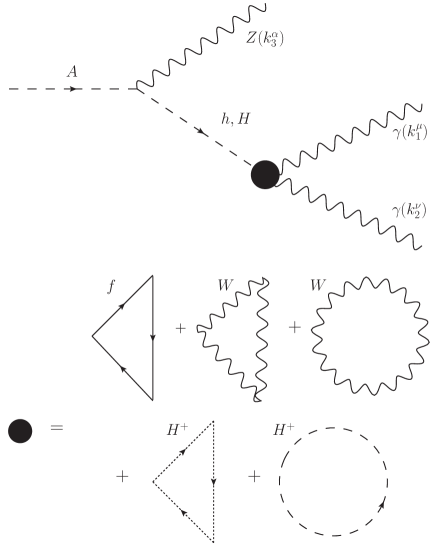
Figure 2: Reducible Feynman diagrams for the $A\to Z\gamma\gamma$ decay in the THDM. For the triangle diagrams there are additional diagrams that are obtained by exchanging the photons. Similar diagrams also contribute to the $\phi\to Z\gamma\gamma$ ($\phi=h,H$) decay, except that the intermediate particle is now the $CP$-odd scalar boson $A$ and there is only contribution from charged fermions in the triangle loop.

As was the case for the box diagram contribution, the reducible diagram contribution is gauge invariant and ultraviolet-finite by its own. It turns out that these diagrams contribute to the gauge-invariant amplitude of Eq. (17) only through the form factor ${\cal F}_{1}$, which includes the contributions of charged fermions, the $W$ gauge boson, and the charged scalar boson $H^{\pm}$

$$\mathcal{F}_{1}^{RD}=\mathcal{F}_{1}^{f}+\mathcal{F}_{1}^{W}+\mathcal{F}_{1}^{H^{\pm}},$$ (18)

with $\mathcal{F}_{1}^{\chi}$ ($\chi=f,{W},{H^{\pm}}$) defined in Appendix A in term of Passarino-Veltman scalar functions.

III.3 $\phi\to Z\gamma\gamma$ ($\phi=h,H$) decay

III.3.1 Box diagram contribution

As for the $\phi\to Z\gamma\gamma$ ($\phi=h,H$) decay, at the one-loop level it also receives the contributions of the fermion box diagrams of Fig. 1 with $A$ replaced by $\phi$. It is worth noting that although a $CP$-even scalar boson does couple to charged $W^{\mp}$ gauge bosons and charged scalar bosons $H^{\mp}$, the corresponding box diagram contributions exactly cancel out due to $CP$ invariance. Notice that the amplitude of this vertex must include the Levi-Civita tensor due to $CP$ invariance, but it cannot arise via box diagrams with charged particles other than charged fermions, whose coupling with the $Z$ gauge boson includes a $\gamma^{5}$ matrix. As the invariant amplitude of a fermion loop includes the trace of a chain of Dirac matrices, the term involving the $\gamma^{5}$ matrix would give rise to the required Levi-Civita tensor.

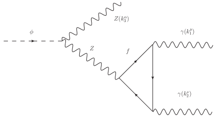
Figure 3: Feynman diagram that also contributes to the $\phi\to Z\gamma\gamma$ ($\phi=h,H$) decay in the THDM, in addition to Feynman diagrams analogue to those of Figs. 1 and 2. The diagram obtained by exchanging the photons is not shown.

The most general Lorentz structure for the $\phi\to Z\gamma\gamma$ ($\phi=h,H$) decay can be written in the following gauge-invariant manifest form

$$\begin{split}\mathcal{M}^{\alpha\mu\nu}(\phi\to Z\gamma\gamma)&=\mathcal{G}_{1}\Big{(}k_{1}\cdot k_{2}\;\epsilon^{\alpha\mu\nu k_{3}}+g^{\mu\nu}\epsilon^{\alpha k_{3}k_{1}k_{2}}-k_{2}^{\mu}\epsilon^{\alpha\nu k_{3}k_{1}}+k_{1}^{\nu}\epsilon^{\alpha\mu k_{3}k_{2}}\Big{)}\\ &+\frac{\mathcal{G}_{2}}{m_{\phi}^{2}}\;\epsilon^{\alpha\mu k_{3}k_{1}}\Big{(}k_{3}\cdot k_{2}\;k_{1}^{\nu}-k_{1}\cdot k_{2}\;k_{3}^{\nu}\Big{)}+\mathcal{G}_{3}\Big{(}k_{1}\cdot k_{2}\;\epsilon^{\alpha\mu\nu k_{1}}+k_{1}^{\nu}\epsilon^{\alpha\mu k_{1}k_{2}}\Big{)}\\ &+\mathcal{G}_{4}\Big{(}k_{3}\cdot k_{2}\;\epsilon^{\alpha\mu\nu k_{1}}+k_{3}^{\nu}\epsilon^{\alpha\mu k_{1}k_{2}}\Big{)}+\Big{(}k_{1}^{\nu}\leftrightarrow k_{2}^{\mu}\Big{)},\end{split}$$ (19)

where we use the shorthand notation $\epsilon^{\alpha kpq}=\epsilon^{\alpha\beta\lambda\rho}k_{\beta}p_{\lambda}q_{\rho}$, etc. Again the form factors $\mathcal{G}_{i}$ depend on $s$, $s_{1}$, $s_{2}$, and $\mu_{Z}$. To arrive to the above equation, we used Schouten’s identity. These form factors receive contributions from both box diagrams and reducible diagrams: $\mathcal{G}_{i}=\mathcal{G}_{i}^{Box}+\mathcal{G}_{i}^{RD}$. As far as the contributions from the box diagrams are concerned, they are reported in Appendix B in terms of Passarino-Veltman scalar functions.

III.3.2 Reducible diagram contribution

There are also contributions from reducible diagrams that are analogue to those depicted in Fig. 2, but with the photons emerging from the intermediate $CP$-odd scalar boson $A$ via loops of charged fermions only. There are also extra reducible diagrams arising from the process $\phi\to ZZ^{*}\to Z\gamma\gamma$, as shown in Fig. 3. This diagram involves the well-known triangle anomaly $Z^{*}\gamma\gamma$, which receives contributions from charged fermions only. This is due to $CP$ invariance as the amplitude for this vertex must be proportional to the Levi-Civita tensor, which can only arise via the trace of a chain of Dirac matrices including $\gamma^{5}$, which in turn only is present in a fermion loop. Therefore loops of the charged $W$ gauge boson or the charged scalar boson do not contribute to this vertex. Also, due to the Landau-Yang theorem, the $Z^{*}\gamma\gamma$ vertex vanishes for real $Z$, so this diagram does not contribute to the $\phi\to Z\gamma\gamma$ decay when the $\phi$ scalar boson is kinematically allowed to decay into a pair of real $Z$ gauge bosons. These reducible Feynman diagrams only contribute to the invariant amplitude of the $\phi\to Z\gamma\gamma$ ($\phi=h,H$) decay via the form factor $\mathcal{G}_{3}$:

$$\mathcal{G}_{3}^{RD}=\mathcal{G}_{3}^{Z}+\mathcal{G}_{3}^{A},$$ (20)

where $\mathcal{G}_{3}^{Z}$ and $\mathcal{G}_{3}^{A}$ are the form factors arising from the diagrams with the vertices $Z^{*}\gamma\gamma$ and $A^{*}\gamma\gamma$, respectively. Explicit expressions in terms of Passarino-Veltman scalar functions are given in Appendix B. Note that we must include the contribution of all fermion families in order to cancel the $Z^{*}\gamma\gamma$ anomaly.

III.4 $A\to Z\gamma\gamma$ and $\phi\to Z\gamma\gamma$ ($\phi=h,H$) decay widths

There are two scenarios for the $\phi_{i}\to Z\gamma\gamma$ ($\phi=h,H,A$) decays, which depend on the value of the mass of the incoming scalar boson $\phi_{i}$ as compared to the mass of the exchanged scalar boson, which we denote by $\phi_{e}$: $\phi_{e}=h,H$ for $\phi_{i}=A$ or $\phi_{e}=A$ for $\phi_{i}=h,H$. We will present the expression for the resulting decay width in both scenarios.

III.4.1 $m_{\phi_{i}}<m_{\phi_{e}}+m_{Z}$

In this scenario, the incoming scalar boson $\phi_{i}$ will not be heavy enough to produce an on-shell $\phi_{e}$ in addition to the on-shell $Z$ gauge boson. Therefore we will have a pure three-body decay induced by both box and reducible diagrams. The corresponding decay width can be written as

$$\Gamma(\phi_{i}\rightarrow Z\gamma\gamma)=\dfrac{m_{\phi_{i}}}{256\;\pi^{3}}\int_{x_{1i}}^{x_{1f}}\int_{x_{2i}}^{x_{2f}}|\overline{\mathcal{M}}(\phi_{i}\rightarrow Z\gamma\gamma)|^{2}dx_{2}\;dx_{1},$$ (21)

where we introduced the following scaled variables

$$x_{1} =\frac{2p\cdot k_{3}}{m_{\phi_{i}}^{2}}=1+\mu_{Z}-\hat{s},$$ (22)

$$x_{2} =\frac{2p\cdot k_{1}}{m_{\phi_{i}}^{2}}=1-\hat{s}_{2},$$ (23)

$$x_{3} =\frac{2p\cdot k_{2}}{m_{\phi_{i}}^{2}}=1-\hat{s}_{1},$$ (24)

with $\hat{s}=s/m_{\phi_{i}}^{2}$ and $\hat{s}_{i}=s_{i}/m_{\phi_{i}}^{2}$. In the center-of-mass frame of the decaying $\phi_{i}$ we have $x_{1}=2E_{Z}/m_{\phi_{i}}$, $x_{2}=2E_{\gamma}/m_{\phi_{i}}$, and $x_{3}=2E_{\gamma^{\prime}}/m_{\phi_{i}}$, where $E_{\gamma}$ ($E_{\gamma^{\prime}}$) stands for the energy of the photon with four-momentum $k_{1}$ ($k_{2}$). From energy conservation, these variables obey $x_{1}+x_{2}+x_{3}=2$.

The kinematic limits in Eq. (21) are as follows

$$\begin{split}x_{1i}&=2\sqrt{\mu_{Z}},\\ x_{1f}&=1+\mu_{Z},\\ x_{2i,2f}&=\dfrac{1}{2}\left(2-x_{1}\mp\sqrt{x_{1}^{2}-4\mu_{Z}}\right).\end{split}$$ (25)

The squared average amplitudes for both decays $A\to Z\gamma\gamma$ and $\phi\to Z\gamma\gamma$ ($\phi=h,H$) are presented in Appendix C.

III.4.2 $m_{\phi_{i}}>m_{\phi_{e}}+m_{Z}$

In this scenario the incoming scalar boson $\phi_{i}$ is heavy enough to produce an on-shell scalar boson $\phi_{e}$. Therefore the $\phi_{i}\to Z\gamma\gamma$ decay proceeds as the pure two-body decay $\phi_{i}\to Z\phi_{e}$, followed by the decay $\phi_{e}\to\gamma\gamma$. Note that in the case of the decay of a $CP$-even Higgs boson, although the decay into a pair of real $Z$ gauge bosons will now be kinematically allowed, the $Z\to\gamma\gamma$ decay is forbidden by the Landau-Yang theorem, which means that the contribution of the intermediary $Z$ gauge boson will thus vanish. In this scenario, using the Breit-Wigner propagator for the exchanged scalar boson, Eq. (21) can be integrated and the $\phi_{i}\to Z\gamma\gamma$ decay width can be written as

$$\Gamma(\phi_{i}\to Z\gamma\gamma)=\Gamma(\phi_{i}\to Z\phi_{e})\mbox{BR}(\phi_{e}\to\gamma\gamma),$$ (26)

with the decay width $\Gamma(\phi_{e}\to\gamma\gamma)$ given by

$$\Gamma(\phi_{e}\to\gamma\gamma)=\frac{\alpha^{2}g^{2}m_{\phi}^{3}}{1024\pi^{3}m_{W}^{2}}\left|\mathcal{F}^{\phi_{e}\gamma\gamma}\right|^{2}.$$ (27)

For a $CP$-even scalar boson $\phi_{e}=h,H$, $F^{\phi_{e}\gamma\gamma}$ receive contributions from charged fermions, the charged $W$ gauge boson, and the charged scalar boson $H^{\pm}$:

$$\mathcal{F}^{\phi_{e}\gamma\gamma}=\mathcal{F}^{\phi_{e}\gamma\gamma}_{f}(\tau_{f})+\mathcal{F}^{\phi_{e}\gamma\gamma}_{W}(\tau_{W})+\mathcal{F}^{\phi_{e}\gamma\gamma}_{H^{\pm}}(\tau_{H^{\pm}})\,\quad{\rm for}\quad\phi_{e}=h,H,$$ (28)

with $\tau_{\chi}=4m_{\chi}^{2}/m_{\phi_{e}}^{2}$. The $\mathcal{F}^{\phi_{e}\gamma\gamma}_{\chi}(x)$ functions can be obtained from the results for the reducible diagrams presented in Appendix B by setting $s=m_{\phi_{e}}^{2}$. They are given by

$$\mathcal{F}^{\phi_{e}\gamma\gamma}_{\chi}(\tau_{\chi})=\left\{\begin{array}[]{cl}\sum_{f}g_{\phi_{e}\bar{f}f}N_{c}^{f}Q_{f}^{2}\left[-2\tau_{f}(1+(1-\tau_{f})f(\tau_{f}))\right]&\quad\chi=f,\\ \\ g_{\phi_{e}WW}\left[2+3\tau_{W}+3\tau_{W}(2-\tau_{W})f(\tau_{W})\right]&\quad\chi=W,\\ \\ \dfrac{m_{W}^{2}(1-2s_{W}^{2})g_{\phi_{e}H^{-}H^{+}}}{c_{W}^{2}m_{H^{\pm}}^{2}}\left[\tau_{H^{\pm}}(1-\tau_{H^{\pm}}f(\tau_{H^{\pm}}))\right]&\quad\chi=H^{\pm},\end{array}\right.$$ (29)

for $\phi_{e}=h,H$ $f(x)$ is given by

$$f(x)=\left\{\begin{array}[]{cr}\left[\arcsin\left(\frac{1}{\sqrt{x}}\right)\right]^{2}&x\geq 1,\\ -\frac{1}{4}\left[\log\left(\frac{1+\sqrt{1-x}}{1-\sqrt{1-x}}\right)-i\pi\right]^{2}&x<1.\end{array}\right.$$ (30)

On the other hand, when the intermediary scalar boson is the $CP$-odd one $A$, we only have the contributions of charged fermions

$$\mathcal{F}^{A\gamma\gamma}=\mathcal{F}^{A\gamma\gamma}_{f}(\tau_{f})=\sum_{f}g_{A\bar{f}f}Q_{f}^{2}N_{c}^{f}\left[-2\tau_{f}f(\tau_{f})\right].$$ (31)

As for the $\phi_{i}\to\phi_{e}Z$ decay width, it is given as follows

$$\Gamma(\phi_{i}\to Z\phi_{e})=\frac{g_{\phi Z\phi_{e}}^{2}\,\alpha\,m_{\phi_{i}}^{3}}{256s_{W}^{2}}\Bigl{(}(4-(\sqrt{\tau_{\phi_{e}}}-\sqrt{\tau_{Z}})^{2})(4-(\sqrt{\tau_{\phi_{e}}}+\sqrt{\tau_{Z}})^{2})\Bigr{)}^{\frac{3}{2}}.$$ (32)

Note that $\tau_{\phi_{e}}=4m_{\phi_{e}}^{2}/m_{\phi_{i}}^{2}$, thus $\tau_{\phi_{e}}=4m_{\phi}^{2}/m_{A}^{2}$ for $A\to Z\gamma\gamma$ and $\tau_{\phi_{e}}=4m_{A}^{2}/m_{\phi}^{2}$ for $\phi\to Z\gamma\gamma$ ($\phi=h,H$). A similar expression with the corresponding replacements is obeyed by the $\phi_{e}\to W^{\pm}H^{\mp}$ decays if kinematically allowed.

All the necessary coupling constants $g_{\phi\bar{f}f}$, $g_{\phi WW}$, $g_{\phi ZZ}$, $g_{\phi AZ}$, $g_{\phi W^{\pm}H^{\mp}}$, $g_{\phi H^{-}H^{+}}$ $(\phi=h,H)$, along with $g_{A\bar{f}f}$ and $g_{AW^{\pm}H^{\mp}}$ are shown in Table 2 of Appendix A. Other coupling constants involved in decays such as $H\to hh$ and $\phi\to AA$ can be found in Ref. Branco et al. (2012); Gunion et al. (2000) for instance. To obtain the branching ratio $BR(\phi_{e}\to\gamma\gamma)$, we need the main decay widths of both $CP$-even and $CP$-odd scalar bosons, which have already been studied in the literature considerably Gunion et al. (2000). For completeness we present in Appendix D all the necessary formulas, which can also be helpful to obtain the branching ratio for the $\phi_{i}\to Z\gamma\gamma$ decay in type-II THDM and make a comparison with that of other decay channels.

IV Numerical Analysis and Results

We now turn to the numerical analysis. To begin with, we will analyze the current constraints on the parameter space of type-II THDM.

IV.1 Allowed parameter space of type-II THDM

After the Higgs boson discovery, several studies have been devoted to explore the implications on the parameter space of THDMs Grinstein and Uttayarat (2013); Dumont et al. (2014); Dorsch et al. (2016); Wang et al. (2017); Eberhardt et al. (2013). From the recent analyses of the ATLAS and CMS collaborations Aad et al. (2016), it is inferred that the properties of the $125$ GeV scalar boson found at the LHC are highly consistent with the SM predictions, thereby imposing strong constraints on the scalar sector of SM extensions. If one of such theories predicts several $CP$-even physical Higgs bosons, one of them must correspond to the SM one and reproduce its couplings to fermions and gauge bosons. In type-II THDM, the scalar boson $h$ is usually assumed to be the lightest one and so is identified with the SM Higgs boson, which constrains the parameter space of the model to a region very close to the alignment limit $\sin(\beta-\alpha)=1$, where the heavy Higgs $H$ does not couple to the gauge bosons and the coupling $hZA$ is absent at tree-level Aad et al. (2015); Eberhardt et al. (2013); Pich and Tuzon (2009). The couplings of the $h$ Higgs boson to the fermions involve the mixing angles $\alpha$ and $\beta$. Therefore, the LHC data can impose strong constraints on both parameters. Other constraints can be obtained from theoretical requirements such as vacuum stability and unitarity of the scalar potential as well as perturbativity of the Higgs couplings. Also, the oblique parameters $S,T$ and $U$ can impose strong constraints on the masses of the new Higgs bosons $A$ and $H$, requiring that at least one of them is very heavy: a $CP$-odd scalar with $m_{A}\sim 200$ GeV requires a heavy $CP$-even scalar with $m_{H}\geq 600$ GeV and viceversa. As for the charged Higgs boson mass, it can be constrained through experimental measurements on low energy FCNC processes.

All of the above constraints can be complemented with the direct searches of additional Higgs bosons at LEP and the LHC. Below we present the constraints most relevant for our numerical analysis.

• Mixing angles $\beta$ and $\beta-\alpha$: since the $h$ Higgs boson is identified with the SM Higgs boson, the LHC data restrict $\beta-\alpha$ to lie very close to $\pi/2$, namely, $|\sin(\beta-\alpha)|>0.999$, with a small interval around $t_{\beta}=1$ where such a constraint is less stringent. Furthermore, in type-II THDM, for $\beta-\alpha\simeq\pi/2$, the scalar couplings to the top quark (bottom quark) behaves as $1/t_{\beta}$ ($t_{\beta}$), thus FCNCs process are very sensitive to small and large values of $t_{\beta}$, which will impose stringent constraints on this parameter. We can thus consider values of $t_{\beta}$ in the range 1-30.

• Mass of the charged Higgs boson $m_{H^{\pm}}$: while the direct search at LEP imposed the constraint $m_{H^{\pm}}>80$ GeV Abbiendi et al. (2013), the measurement of the $\bar{B}\to X_{s}\gamma$ branching ratio imposes the very stringent bound $m_{H^{\pm}}>570$ GeV, for $t_{\beta}\sim 1.5$ Misiak and Steinhauser (2017).

• Mass of the $CP$-odd scalar $m_{A}$: the authors of Ref. Wang et al. (2017) examine the scenarios where either $m_{A}$ or $m_{H}$ is set to a large value about 600-700 GeV while the other one is bounded via theory constraints and experimental data, with the remaining free parameters set to the values mentioned above. We will follow closely this analysis as it is of interest for the present work. We first examine the case of a light $CP$-odd scalar and a heavy $CP$-even scalar with mass $m_{H}=600$ GeV. In this scenario the searches for the decays $A\to\bar{\tau}\tau$, $A\to\gamma\gamma$, and $A\to hZ$ exclude the region $m_{A}<350$ GeV, whereas the LHC data on the Higgs boson require $m_{A}$ to be larger than $220$ GeV. On the other hand, the search for the channel $b\bar{b}\to A\to\bar{\tau}\tau$ allows for $m_{A}$ values in the range 350-700 GeV and impose the upper limit $t_{\beta}<2$ for $m_{A}\leq 500$ GeV, whereas $t_{\beta}<15$ for $m_{A}\leq$ 500 GeV.

• Mass of the heavy $CP$-even scalar $m_{H}$: we now examine the scenario with a light $CP$-even scalar and a heavy $CP$-odd scalar with $m_{A}=700$ GeV. In this case the whole constraints require $m_{H}>300$ GeV, whereas the $b\bar{b}\to H/A\to\tau\bar{\tau}$ channel imposes an upper bound on $t_{\beta}$ as a function of $m_{H}$. For instance, for $m_{H}=200$ (600) GeV $t_{\beta}<6$ (15). On the other hand, the searches for the $H$ decays into $\bar{\tau}\tau$, $WW$, $ZZ$, $\gamma\gamma$, and $hh$ require $\tan\beta>2.5$ for $m_{H}<380$ GeV. For a lighter $m_{A}=600$ GeV, the search for the $A\to HZ$ channel can exclude the region $m_{H}<270$ GeV.

We now turn to study the behavior of the $A\to Z\gamma\gamma$ and $\phi\to Z\gamma\gamma$ ($\phi=h,H$) branching ratios as functions of the parameters $t_{\beta}$, $\beta-\alpha$, $m_{H^{\pm}}$, $m_{A}$ and $m_{H}$. We stick to the still allowed values for these parameters, whereas for the SM parameters we take the values given in Ref. Patrignani et al. (2016). For our analysis we used the LoopTools package van Oldenborgh and Vermaseren (1990); Hahn and Perez-Victoria (1999) for the numerical evaluation of the Passarino-Veltman scalar functions appearing in the decay amplitudes. The dominant decay widths of the $CP$-odd and $CP$-even scalar bosons were evaluated by our own Mathematica code that implements the formulas of Appendix D, including the QCD corrections for the decays into light quarks.

IV.2 $A\to Z\gamma\gamma$ branching ratio

We work in a region close to the alignment limit and use $\sin(\beta-\alpha)=0.999$. In this scenario, the strength of the $hZA$ vertex is negligible and so the contributions to the $A\to Z\gamma\gamma$ decay only arise from box diagrams and reducible diagrams with $H$ exchange, which receive their main contributions from the top and bottom quarks. The contribution of the loops with $W$ gauge bosons turns out to be negligibly small as it is proportional to $\cos^{2}(\beta-\alpha)$, whereas the charged scalar boson also gives a very small contribution for $m_{H^{\pm}}$ of the order of a few hundred GeVs.

We can distinguish two scenarios of interest: $m_{A}<m_{H}+m_{Z}$ and $m_{A}>m_{H}+m_{Z}$. Below we examine the behavior of the $A\to Z\gamma\gamma$ branching ratio in such scenarios.

IV.2.1 Scenario with $m_{A}<m_{H}+m_{Z}$

We consider the scenario with $m_{H}=600$ GeV and analyze the behavior of $BR(A\to Z\gamma\gamma)$ as a function of $m_{A}$ in the range $350-650$ GeV. For the mixing angle $\beta$ we consider two values: $t_{\beta}=2$ and $t_{\beta}=10$, which are allowed for $m_{A}<500$ GeV and 500 GeV $\leq m_{A}\leq 700$ GeV, respectively. In the upper plots of Fig. 4 we show the behavior of the $A\to Z\gamma\gamma$ branching ratio as function of $m_{A}$ for the two chosen values of $t_{\beta}$. We also show the main decay modes of the $CP$-odd scalar boson: $A\to b\bar{b}$, $A\to W^{-}H^{+}$, $t\bar{t}$, $gg$, $\gamma\gamma$, and $Z\gamma$. The decay $A\to Zh$ has a negligible branching ratio in the region close to the alignment limit and is not shown in the plots. We note that the main contribution to $BR(A\to Z\gamma\gamma)$ arises from the reducible diagrams with top quarks, whereas the contribution of the loops with charged scalar bosons is negligible. Since in this scenario the intermediary scalar boson $H$ is far from the resonance, the reducible diagram contribution is very small, though it is larger than the box diagram contribution by almost two orders of magnitude. Therefore, the $Z\to A\gamma\gamma$ branching ratio is thus very small. For instance, for $t_{\beta}=2$, $BR(A\to Z\gamma\gamma)$ is of the order of $10^{-11}$ for $m_{A}=300$ GeV with a small increase as $m_{A}$ increases. When $t_{\beta}$ increases up to $10$, $BR(A\to Z\gamma\gamma)$ decreases about one order of magnitude as the top quark contribution is suppressed by a factor of $1/t_{\beta}$. In this region of the parameter space of the type-II THDM, the $A\to Z\gamma\gamma$ branching ratio is considerably smaller than those of the one-loop induced decays $A\to\gamma\gamma$ and $A\to Z\gamma$.

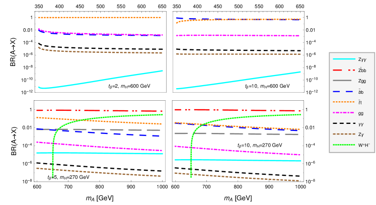
Figure 4: Branching ratio for the $A\to Z\gamma\gamma$ decay in type-II THDM as a function of $m_{A}$ for $m_{H^{\pm}}=570$ GeV, $\sin(\beta-\alpha)=0.999$, and two values of $t_{\beta}$ allowed by theory and experimental constraints. In the upper (lower) plots we use $m_{H}=600$ (270) GeV. The branching ratios for the main $A$ decay channels are also shown.

IV.2.2 Scenario with $m_{A}>m_{H}+m_{Z}$

We now turn to analyze the scenario where the $CP$-even scalar is relatively light, with a mass $m_{H}=270$ GeV along with a heavier $CP$-odd scalar with a mass in the range 600-1000 GeV. We use $t_{\beta}=5$ and $t_{\beta}=10$, which are allowed for $m_{A}=600$ GeV and $m_{A}=700$ GeV, respectively. In this scenario the intermediate scalar boson $H$ is on resonance and the $CP$-odd scalar can decay as $A\to ZH$ with a large branching ratio. The decay $A\to Z\gamma\gamma$ would then proceed in two stages: after the $CP$-odd scalar boson decays as $A\to ZH$, the on-shell $CP$-even scalar boson decays into a photon pair $H\to\gamma\gamma$, namely, $A\to HZ\to Z\gamma\gamma$. The enhancement of $BR(A\to Z\gamma\gamma)$ becomes evident in the lower plots of Fig. 4, where we show its behavior as a function of $m_{A}$, along with that of the branching ratios of other decay modes of the $CP$-odd scalar boson. We observe that $BR(A\to Z\gamma\gamma)$ increases up to four orders of magnitude with respect to the result obtained in the scenario with $m_{A}<m_{H}+m_{Z}$ and can reach values of the order of $10^{-6}-10^{-5}$ when $m_{A}$ is in the 600-800 GeV range. In this mass regime, the main decay is $A\to HZ$, which explains why the $A\to Z\gamma\gamma$ decay has such an enhanced branching ratio. For illustrative purpose we also show the branching ratios for the decays $A\to Z\bar{b}b$ and $A\to Zgg$, which arise from the decay $A\to HZ$ followed by the decays $H\to\bar{b}b$ and $H\to gg$. We note that the dominant decay channel is $A\to Z\bar{b}b$.

The above-described behavior of $BR(A\to Z\gamma\gamma)$ is best illustrated in the contour plot on the $m_{A}$ vs $m_{H}$ plane shown in Fig. 5 for two values of $t_{\beta}$. We observe that $BR(A\to Z\gamma\gamma)$ can reach its largest values, of the order of $10^{-5}$, in the region where $m_{A}>m_{A}+m_{Z}$, whereas it is negligible when $m_{A}<m_{A}+m_{Z}$. Since the $A\to Z\gamma\gamma$ decay receives its main contribution from the loops with top quark, it decreases as $t_{\beta}$ increases.

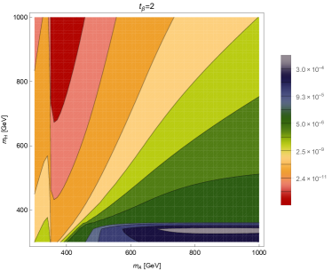
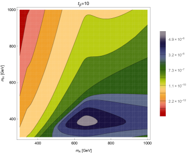
Figure 5: Contour plot of $BR(A\to Z\gamma\gamma)$ in the $m_{A}$ vs $m_{H}$ plane for $\sin(\beta-\alpha)=0.999$, $m_{H^{\pm}}>m_{A}$ and two values of $t_{\beta}$.

IV.3 $H\to Z\gamma\gamma$ branching ratio

We now analyze the behavior of the $H\to Z\gamma\gamma$ branching ratio as a function of $m_{H}$ in scenarios analogue to those discussed for the $CP$-odd scalar boson. For $\sin(\beta-\alpha)=0.999$, apart from the box diagram contribution, the only contribution from reducible diagrams is that with an intermediary $CP$-odd scalar boson $A$, which receives contributions mainly from the top and bottom quarks. The diagram mediated by the $Z$ gauge boson gives a negligible contribution since the $HZZ$ vertex is proportional to $\cos(\beta-\alpha)$.

IV.3.1 Scenario with $m_{H}<m_{A}+m_{Z}$

We consider a heavy $CP$-odd scalar with a mass $m_{A}=600$ GeV and take $m_{H}$ in the range 300-600 GeV. For $t_{\beta}$ we use the values 3 and 10. In the upper plots of Fig. 6 we show the branching ratios for the main decay channels of the $H$ scalar boson. We note that the $H\to Z\gamma\gamma$ decay has a very suppressed branching ratio up to five orders of magnitude smaller than the branching ratios of the one-loop induced decays $H\to\gamma\gamma$ and $H\to Z\gamma$. It increases for smaller $t_{\beta}$ but it seems still beyond the reach of detection.

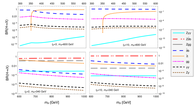
Figure 6: Branching ratio for the $H\to Z\gamma\gamma$ decay in type-II THDM as a function of $m_{H}$ for $m_{H^{\pm}}=570$ GeV, $\sin(\beta-\alpha)=0.999$, and two values of $t_{\beta}$ allowed by theory and experimental constraints. In the upper (lower) plots we use $m_{A}=600$ (350) GeV. The branching ratios for the main $H$ decay channels are also shown.

IV.3.2 Scenario with $m_{H}>m_{A}+m_{Z}$

In this scenario we consider $m_{A}=350$ GeV and take $m_{H}$ in the range 600-1000 GeV. We also use $t_{\beta}=2$ and $t_{\beta}=10$. For the mass of the charged scalar boson we use $m_{H^{\pm}}=575$ GeV as we do not need to assume that $m_{H^{\pm}}>m_{H}$ since the $H\to W^{-}H^{+}$ decay channel has a negligible branching ratio proportional to $\cos(\beta-\alpha)^{2}$. In the lower plots of Fig. 6 we show the $H\to Z\gamma\gamma$ branching ratio along with those of the main decay channels. We note that there is a considerable enhancement of $BR(H\to Z\gamma\gamma)$, up to 5 orders of magnitude, now that the $H\to ZA$ decay is allowed, thus $BR(H\to Z\gamma\gamma)$ can be as large as $10^{-3}$ for $t_{\beta}=2$. Again we include the decays $H\to ZA\to Z\bar{b}b$ and $H\to ZA\to Zgg$, with the dominant decay being the $H\to ZA\to Z\bar{b}b$.

In Fig. 7, we also show the contour plot of $BR(H\to Z\gamma\gamma)$ in the $m_{H}$ vs $m_{A}$ plane for two values of $t_{\beta}$. Again it is evident that $BR(H\to Z\gamma\gamma)$ can reach its largest values when $m_{H}>m_{A}+m_{Z}$ and it is negligible when $m_{H}<m_{A}+m_{Z}$. It also decreases when $t_{\beta}$ increases as it receives the main contribution from loops with the top quark.

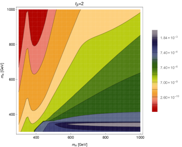
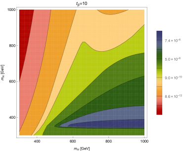
Figure 7: Contour plot of $BR(H\to Z\gamma\gamma)$ in the $m_{H}$ vs $m_{A}$ plane for $\sin(\beta-\alpha)=0.999$, $m_{H^{\pm}}=570$ GeV and two values of $t_{\beta}$.

Finally, we would like to comment shortly on the potential detection of the $A\to Z\gamma\gamma$ and $\phi\to Z\gamma\gamma$ ($\phi=h,H$) decays in the scenario we are considering in type-II THDM. Although there is a considerable enhancement of the corresponding branching ratios, it still seems not enough to put these decays at the reach of experimental detection at the LHC in the near future. In Fig. 8 we show the leading order production cross section for the $CP$-even and $CP$-odd scalar bosons via gluon fusion at the LHC at $\sqrt{s}=$ 14 TeV as a function of the scalar boson mass. It turns out that with an integrated luminosity of 300 fb^-1, to be achieved in LHC run 3, we would have about $1.64\times 10^{5}$ ($3.2\times 10^{5}$) $CP$-even ($CP$-odd) scalar bosons with a mass $m_{\phi}=500$ GeV produced per year, but these numbers drop by one order of magnitude when $m_{\phi}=700$ GeV. For $BR(H\to Z\gamma\gamma)\simeq O(10^{-3})$, we would only have about 164 $H\to Z\gamma\gamma$ events prior to imposing the kinematic cuts, which would render this decay hard to detect. The situation might be more promising at a future high-luminosity 100 TeV $pp$ collider, where we could have thousands of $H\to Z\gamma\gamma$ events prior to imposing the kinematic cuts. As discussed below, this event number would increase in type-I THDM by one order of magnitude as the respective branching ratios would have such an enhancement in that model.

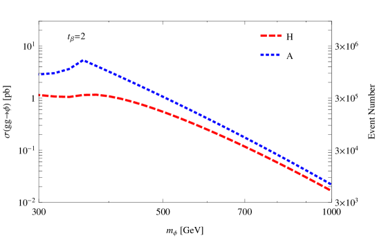
Figure 8: $CP$-even and $CP$-odd scalar boson production cross section via gluon fusion as a function of the scalar boson mass at the LHC at $\sqrt{s}=$ 14 TeV in type-II THDM. We use $\sin(\alpha-\beta)\simeq 0.999$ and $t_{\beta}=2$. The right axis shows the annual event number achieved with an integrated luminosity of 300 fb^-1.

IV.4 $h\to Z\gamma\gamma$ branching ratio

We now briefly discuss the lightest $CP$-even scalar boson decay $h\to Z\gamma\gamma$. Since $h$ must mimic the properties of the SM Higgs boson, it is expected that the $h\to Z\gamma\gamma$ branching ratio does not deviate considerably from its SM value. For $\sin(\beta-\alpha)\simeq 1$, the only contributions arise from box diagrams and the reducible diagram mediated by the $Z$ gauge boson. As mentioned before, the $hZA$ vertex is considerably suppressed, whereas the $hHZ$ one is forbidden due to $CP$ invariance. Even more, there is no enhancement due to the $Z$-mediated reducible diagram since $m_{h}<2m_{Z}$. For $m_{h}=125$ GeV and $t_{\beta}=10$ GeV we obtain $BR(h\to Z\gamma\gamma)\simeq 10^{-9}$, which does not deviate significantly from the SM value Abbasabadi and Repko (2008). Therefore the new physics effects provided by the THDM does not give a significant enhancement to this decay and seem very far from the reach of detection.

IV.5 Kinematic distributions

In the scenario in which the intermediary scalar boson is off-shell, the analysis of the behavior of some kinematic distributions could be helpful to disentangle the decay signal from the potential background. The $Z$ gauge boson energy distribution $d\Gamma(\phi_{i}\to Z\gamma\gamma)/dE_{Z}$ and the photon invariant mass distribution $d\Gamma(\phi_{i}\to Z\gamma\gamma)/dm_{m_{\gamma\gamma^{\prime}}}$ could be useful for this task. To obtain the former, one can plug the relation $dx_{1}=(2/m_{\phi_{i}})dE_{Z}$ into Eq. (21) to obtain

$$\dfrac{d\Gamma(\phi_{i}\to Z\gamma\gamma)}{dE_{Z}}=\dfrac{1}{128\pi^{3}}\int_{x_{2i}}^{x_{2f}}|\overline{\mathcal{M}}(\phi_{i}\to Z\gamma\gamma)|^{2}dx_{2},$$ (33)

where the $Z$ gauge boson energy is defined in the interval $(m_{Z},(m_{\phi_{i}}^{2}+m_{Z}^{2})/(2m_{\phi_{i}}))$.

On the other hand, the expression for the photon invariant mass distribution $d\Gamma(\phi_{i}\to Z\gamma\gamma)/dm_{m_{\gamma\gamma^{\prime}}}$ is obtained using the relation $dm_{\gamma\gamma^{\prime}}=dE_{Z}/\sqrt{\mu_{Z}-x_{1}+1}$, which leads to

$$\dfrac{d\Gamma(\phi_{i}\to Z\gamma\gamma)}{dm_{\gamma\gamma^{\prime}}}=\dfrac{\sqrt{\mu_{Z}-x_{1}+1}}{128\pi^{3}}\int_{x_{2i}}^{x_{2f}}|\overline{\mathcal{M}}(\phi_{i}\to Z\gamma\gamma)|^{2}dx_{2},$$ (34)

where $m_{\gamma\gamma^{\prime}}$ is defined in the interval $(0,m_{\phi_{i}}-m_{Z})$.

For illustrative purpose we show in Fig. 9 the energy distribution $d\Gamma(A\to Z\gamma\gamma)/dE_{Z}$ and the photon invariant mass distribution $d\Gamma(A\to Z\gamma\gamma)/dm_{\gamma\gamma}$ in the alignment limit for $m_{H}=700$ GeV, $m_{H^{\pm}}=750$ GeV, $t_{\beta}=15$, and a few values of $m_{A}$. We observe that in the rest frame of the $CP$-odd scalar, the $Z$ gauge boson energy is peaked at about one half of $m_{A}$. A similar situation is observed for the invariant mass $m_{\gamma\gamma}$.

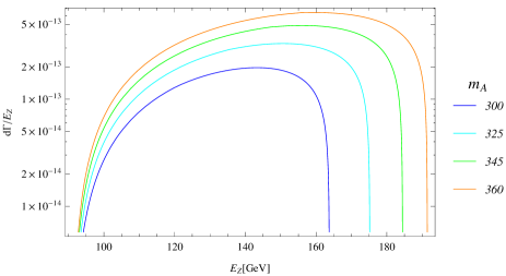
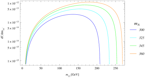
Figure 9: Energy (left plot) and photon invariant mass (right plot) distributions $\Gamma(A\to Z\gamma\gamma)/dE_{Z}$ and $d\Gamma(A\to Z\gamma\gamma)/dm_{\gamma\gamma^{\prime}}$, for several masses of the $CP$-odd scalar boson in type-II THDM. We use $m_{H}=700$ GeV and $t_{\beta}=15$.

IV.6 $A\to Z\gamma\gamma$ and $H\to Z\gamma\gamma$ decays in type-I THDM

We now briefly analyze these decays in the framework of type-I THDM, where the charged scalar boson mass has a lower bound. Since the main contribution to the decays $A\to\gamma\gamma$ and $H\to\gamma\gamma$ arises from the top quark, the effect of a charged Higgs scalar boson with a mass less than $570$ GeV would not have a considerably effect on the decays we are interested in. However, in type-I THDM the couplings of the $CP$-odd scalar boson to both quark types are now proportional to $\cot\beta$, and the same is true for the couplings of $CP$-even scalar bosons in the $\cos(\alpha-\beta)\to 0$ limit . Therefore, the decay widths of the scalar bosons into the $\bar{b}b$ pair would be suppressed for large $t_{\beta}$, which can do have an effect on our decays indeed. Consider for instance the decay $A\to Z\gamma\gamma$ in the scenario where $m_{A}>m_{H}+m_{Z}$. In type-II THDM the main decay channel is $A\to ZH\to Z\bar{b}b$, but for large $t_{\beta}$ this decay would get suppressed in type-I THDM as the $H\to\bar{b}b$ decay gets suppressed. This can translate into an enhancement of the $A\to ZH\to Z\gamma\gamma$ decay width. To analyze this scenario we have performed the explicit calculation of the $A\to Z\gamma\gamma$ and $H\to Z\gamma\gamma$ decay widths in type-I THDM in the same scenarios considered in type-II THDM. The results for the respective branching ratios and those of the main decay channels are shown in Fig. 10, where we observe that the $A\to Z\gamma\gamma$ and $H\to Z\gamma\gamma$ decays can have an enhancement of about one order of magnitude with respect to the values obtained on type-II THDM.

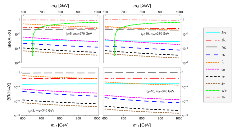
Figure 10: Branching ratios for the $A\to Z\gamma\gamma$ and $H\to Z\gamma\gamma$ decays in type-I THDM as a function of the scalar boson masses for $m_{H^{\pm}}=570$ GeV, $\sin(\beta-\alpha)=0.999$, and two values of $t_{\beta}$ allowed by theory and experimental constraints. The branching ratios for the main decay channels are also shown.

V Conclusions

In this work we have calculated the one-loop contributions to the decays of the $CP$-odd and $CP$-even scalar bosons $A\to Z\gamma\gamma$ and $\phi\to Z\gamma\gamma$ ($\phi=h,H$) in the framework of THDMs. We have presented analytical expressions for both box and reducible diagrams in terms of Passarino-Veltman scalar functions, though the main contributions arise from reducible diagrams. We first discuss the $A\to Z\gamma\gamma$ decay, which has not been discussed previously in the literature to our knowledge. For the numerical analysis we worked within the type-II THDM and considered a region of the parameter space still consistent with experimental data, with $\sin(\beta-\alpha)\simeq 1$, where the lightest $CP$-even scalar boson $h$ is identified with the SM Higgs boson, the $hZA$ vertex has a negligibly small strenght, and the heavy $CP$-even scalar does not couple to the weak gauge bosons. It was found that the $A\to Z\gamma\gamma$ branching ratio is only relevant in the scenario where $m_{A}>m_{H}+m_{Z}$, when the intermediary $H$ boson is on-shell. For $m_{A}>600$ GeV and $t_{\beta}$ close to 1, $BR(A\to Z\gamma\gamma)$ can reach values of the order of $10^{-5}-10^{-4}$, but it decreases by about one order of magnitude as $t_{\beta}$ increases up to 10, which stems from the fact that the dominant contribution arises from the loops with the top quark, which couples to the scalar boson with a strength proportional to $1/t_{\beta}$. On the other hand, when $m_{A}<m_{H}+m_{Z}$, $BR(A\to Z\gamma\gamma)$ is negligibly small, of the order of $10^{-10}$. As far as the $H\to Z\gamma\gamma$ decay is concerned, it exhibits a similar behavior and its branching ratio is non-negligible only in the scenario where $m_{H}>m_{A}+m_{Z}$, when the $CP$-odd scalar is now on-shell. In this region of the parameter space, $BR(H\to Z\gamma\gamma)$ can reach the level of $10^{-4}-10^{-3}$ for $m_{H}>600$ GeV and $t_{\beta}\simeq 1$, but it decreases for larger $t_{\beta}$. We also discussed the $h\to Z\gamma\gamma$ decay, which receives contribution from box diagrams and a reducible diagram mediated by the $Z$ gauge boson. Since the properties of the $h$ scalar boson are nearly identical to the SM Higgs boson, it is found that the $h\to Z\gamma\gamma$ branching ratio does not deviates significantly from the SM prediction and it is of the order of $10^{-9}$. Our calculation is in agreement with previous evaluations. The new physics effects of THDMs are thus not relevant for this decay. Finally we also estimated these rare decays in the framework of type-I THDM, where we find that the respective branching ratios can be enhanced buy about one order of magnitude with respect to those of type-II THDM.

Appendix A Feynman rules

In this appendix we present the Feynman rules necessary for our calculation, which was performed in the unitary gauge. We first present the Feynman rules for the vertices $VW^{-}W^{+}$, $\gamma\gamma W^{-}W^{+}$, and $V\bar{f}f$ ($V=\gamma,Z$), which are identical to the SM ones and are shown in Fig. 11.

Figure 11: SM Feynman rules necessary for our calculation. All the 4-momenta are incoming. $g_{VWW}=1$ ($-\frac{c_{W}}{s_{W}}$) for $V=\gamma$ $(Z)$. In addition $\Gamma^{\alpha\mu\nu}(k_{1},k_{2},k_{3})=(k_{1}-k_{2})^{\nu}g^{\alpha\mu}+(k_{2}-k_{3})^{\alpha}g^{\mu\nu}+(k_{3}-k_{1})^{\mu}g^{\alpha\nu}$ and $\Sigma^{\alpha\beta\mu\nu}=2g^{\alpha\beta}g^{\mu\nu}-g^{\alpha\mu}g^{\beta\nu}-g^{\alpha\nu}g^{\beta\mu}$. We also need the Feynman rules for the interactions of the photon and the $Z$ gauge boson with a fermion pair, which are as follows: $-ieQ_{f}\gamma^{\mu}$ and $-i\frac{g}{2c_{W}}(g_{V}^{f}-g_{A}^{f}\gamma^{5})\gamma^{\mu}$, respectively, where $g_{A}^{f}=\frac{1}{2}T^{3}_{f}$ and $g_{V}^{f}=\frac{1}{2}T_{3}^{f}-Q_{f}s_{W}^{2}$, with $Q_{f}$ the fermion charge and $T^{3}_{f}=1$ ($-1$) for up quarks (down quarks and charged leptons) . 

We also need the couplings of the neutral Higgs bosons to the fermions, the gauge bosons, and the charged scalar bosons. The Feynman rules for the couplings of the neutral Higgs bosons to fermion pairs in THDMs are shown in Fig. 12, and the corresponding coupling constants for type-II THDM are presented and Table 2 Branco et al. (2012).

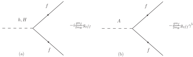
Figure 12: Feynman rules for the couplings of the scalar bosons to fermions in THDMs. The corresponding coupling constants for type-II THDM are shown in Table 2.

Table 2: Constants for the couplings of the scalar bosons to fermions and gauge bosons in type-II THDM as described in Figs. 12 and 13. We have used the short-hand notation $s_{a}=\sin a$ and $c_{a}=\cos a$. The $g_{\phi ZZ}$ couplings obey $g_{\phi ZZ}=\frac{1}{c_{W}^{2}}g_{\phi WW}$ Branco et al. (2012).

$\phi$	$g_{\phi uu}$	$g_{\phi dd}$ ($g_{\phi ll}$)	$g_{\phi WW}$	$g_{\phi ZA}$	$g_{\phi H^{-}H^{+}}$	$g_{\phi W^{-}H^{+}}$
$h$	$-\left(s_{\beta-\alpha}+\dfrac{c_{\beta-\alpha}}{t_{\beta}}\right)$	$-\left(s_{\beta-\alpha}-t_{\beta}c_{\beta-\alpha}\right)$	$s_{\beta-\alpha}$	$c_{\beta-\alpha}$	$\left(c_{W}c_{\beta-\alpha}-\frac{1}{2c_{W}}c_{2\beta}c_{\beta+\alpha}\right)$	$c_{W}s_{\beta-\alpha}$
$H$	$-\left(c_{\beta-\alpha}-\dfrac{s_{\beta-\alpha}}{t_{\beta}}\right)$	$-\left(c_{\beta-\alpha}+t_{\beta}s_{\beta-\alpha}\right)$	$c_{\beta-\alpha}$	$-s_{\beta-\alpha}$	$\left(c_{W}s_{\beta-\alpha}+\frac{1}{2c_{W}}c_{2\beta}s_{\beta+\alpha}\right)$	$c_{W}c_{\beta-\alpha}$
$A$	$\dfrac{1}{t_{\beta}}$	$t_{\beta}$	$0$	$0$	$0$	$-ic_{W}$

As far as the couplings of scalar bosons to gauge bosons, we must expand the covariant derivative of Eq. (2) in terms of the physical fields. It is straightforward to obtain the Feynman rules shown in Fig. 13 for the couplings $\phi VV$ ($V=W,Z$) and $Z\phi A$ ($\phi=h,H$). Note that the $AVV$ ($V=W,Z$) and $HhZ$ couplings are absent due to $CP$ conservation. Other Feynman rules such as those for the vertices $\gamma H^{-}H^{+}$, $ZH^{-}H^{+}$, and $\gamma\gamma H^{-}H^{+}$ are also obtained from the Higgs kinetic sector and are shown in Fig. 13, and so is the Feynman rule for the couplings of the $CP$-even scalar bosons to a pair of charged scalar boson $\phi H^{-}H^{+}$, which emerge from the Higgs potential (3) once it is diagonalized.

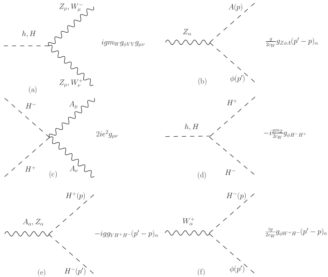
Figure 13: Feynman rules necessary for our calculation in THDMs. All the four-momenta are incoming. Here $\phi=h,H$ in diagram (b) but $\phi=h,H,A$ in diagram (f). Also, in diagram (e) $g_{AH^{+}H^{-}}=s_{W}$ and $g_{ZH^{+}H^{-}}=c_{2W}/{2c_{W}}$. The remaining coupling constants for type-II THDM are presented in Table 2.

Appendix B $A\to Z\gamma\gamma$ and $\phi\to Z\gamma\gamma$ ($\phi=h,H)$ decay amplitudes

We now present the form factors of Eqs. (17) and (19) in terms of Passarino-Veltman scalar functions.

B.1 $A\to Z\gamma\gamma$ decay

B.1.1 Box diagrams

Box diagrams give the following contributions to the form factors of Eq. (17)

$$\mathcal{F}_{i}^{Box}=\sum_{f}\frac{16g^{f}_{A}g_{A\bar{f}f}g^{2}\alpha m_{f}^{2}Q_{f}^{2}N_{c}^{f}}{m_{W}c_{W}sX_{A}^{2}}f_{i}^{Box},$$ (35)

with

$$\begin{split}f_{1}^{Box}&=s\Bigl{[}X_{A}\Delta_{2Z}+sm_{Z}^{2}(s_{1}+s_{2})\Bigr{]}C_{1}(s)+{\frac{\Delta_{2A}}{s}}\Delta_{2Z}\Bigl{[}s_{2}\Delta_{1Z}^{2}-m_{Z}^{2}\Delta_{2A}^{2}\Bigr{]}C_{2}(s_{2})+{\frac{\Delta_{1A}}{s}}\Bigl{[}s_{1}(s_{1}+s)\Delta_{2Z}^{2}\\ &+[m_{A}^{2}(2s_{1}+s)(s_{1}-\Delta_{2Z})+(m_{Z}\Delta_{1A})^{2}-(s_{1}s+(s_{1}+s)^{2})s_{1}]m_{Z}^{2}\Bigr{]}C_{2}(s_{1})-\Delta_{1Z}^{2}\Bigl{[}\Delta_{2Z}\Bigl{(}m_{Z}^{2}-{\frac{X_{A}}{s}}\Bigr{)}\\ &+sm_{Z}^{2}\Bigr{]}C_{3}(s_{1})+\Delta_{2A}\Delta_{2Z}^{2}\Bigl{[}m_{Z}^{2}-{\frac{X_{A}}{s}}\Bigr{]}C_{3}(s_{2})+sm_{Z}^{2}\Bigl{[}(s_{1}-s_{2})^{2}+X_{A}\Bigr{]}C_{4}(s)+{\frac{s}{2}}\Bigl{[}m_{A}^{2}m_{Z}^{2}(s_{1}(\Delta_{1Z}\\ &+s_{1}-s_{2})-2X_{A})+s_{1}^{2}(2m_{Z}^{4}-(2s_{1}+s_{2})m_{Z}^{2}+s_{2}^{2})+\Bigl{(}m_{Z}^{2}-{\frac{X_{A}}{s}}\Bigl{)}4m_{f}^{2}X_{A}\Bigr{]}D_{1}(s_{1})-{\frac{s}{2}}\Bigl{[}s_{1}s_{2}^{3}\\ &-s_{2}m_{Z}^{2}(s_{2}(\Delta_{2Z}+s_{1}+3s)+X_{A})-4Xm_{f}^{2}\Bigl{(}m_{Z}^{2}-{\frac{X_{A}}{s}}\Bigr{)}\Bigr{]}D_{1}(s_{2})+{\frac{1}{2}}\Bigl{[}s_{2}s^{2}(s_{2}-4m_{f}^{2})(m_{Z}^{2}+s_{2})\\ &+\Delta_{2A}\Delta_{2Z}\Bigl{(}{\frac{2\Delta_{2A}^{2}}{s}}\Delta_{2Z}^{2}-\Delta_{2A}(4m_{f}^{2}-m_{Z}^{2}-5s_{2})\Delta_{2Z}+2(s_{2}-2m_{f}^{2})(m_{Z}^{2}+2s_{2})s\Bigr{)}\Bigr{]}D_{2}(s_{2}),\end{split}$$ (36)

$$\begin{split}f_{2}^{Box}&=\frac{X_{A}}{2}\Bigl{(}2\Delta_{2A}\Bigl{(}sC_{1}(s)+\Delta_{1A}C_{2}(s_{1})+{\frac{\Delta_{2Z}}{2}}C_{3}(s_{2})\Bigr{)}+sm_{A}^{2}\Delta_{1Z}D_{1}(s_{1})\\ &+\Delta_{1Z}X_{A}D_{2}(s_{2})-s\Big{[}X_{A}+s_{2}\Delta_{2A}\Big{]}D_{1}(s_{2})\Bigr{)},\end{split}$$ (37)

and

$$\begin{split}f_{3}^{Box}&=2sm_{A}^{2}\Big{[}X_{A}+s(s_{1}+s_{2})\Big{]}C_{1}(s)+2ss_{1}\Delta_{1A}C_{2}(s_{1})-2\Delta_{2A}^{2}\Delta_{2Z}C_{2}(s_{2})\\ &-2\Delta_{1Z}^{2}\Delta_{1A}C_{3}(s_{1})+2ss_{2}\Delta_{2Z}C_{3}(s_{2})-2s\Bigl{[}X_{A}+(s_{1}-s_{2})^{2}\Bigr{]}C_{4}(s)-X_{A}\Bigl{[}X_{A}+4sm_{f}^{2}\Bigr{]}D_{2}(s_{2})\\ &-s\Big{[}s_{1}(X_{A}+2s_{1}s)+4X_{A}m_{f}^{2}\Big{]}D_{1}(s_{1})-s\Big{[}s_{2}(X_{A}+2s_{2}s)+4X_{A}m_{f}^{2}\Bigr{]}D_{1}(s_{2}),\end{split}$$ (38)

where the kinematical invariant variables $s_{1}$, $s_{2}$ and $s$ were defined in Eqs. (13)-(15). In addition, we use the following auxiliary variables:

$$\Delta_{ij} = s_{i}-m_{j}^{2},$$ (39a)

$$X_{\chi} = s_{1}s_{2}-m_{Z}^{2}m_{\chi}^{2},$$ (39b)

for $i=1,2$ and $j=A,Z$. As for the three- and four-point Passarino-Veltman scalar functions $C_{i}$ and $D_{i}$, they are defined as

$$\begin{split}C_{1}(p^{2})&=C_{0}(0,0,p^{2},m_{f}^{2},m_{f}^{2},m_{f}^{2}),\\ C_{2}(p^{2})&=C_{0}(0,p^{2},m_{A}^{2},m_{f}^{2},m_{f}^{2},m_{f}^{2}),\\ C_{3}(p^{2})&=C_{0}(m_{Z}^{2},0,p^{2},m_{f}^{2},m_{f}^{2},m_{f}^{2}),\\ C_{4}(p^{2})&=C_{0}(m_{Z}^{2},p^{2},m_{A}^{2},m_{f}^{2},m_{f}^{2},m_{f}^{2}),\\ D_{1}(p^{2})&=D_{0}(m_{Z}^{2},0,0,m_{A}^{2},p^{2},s,m_{f}^{2},m_{f}^{2},m_{f}^{2},m_{f}^{2}),\\ D_{2}(p^{2})&=D_{0}(m_{Z}^{2},0,m_{A}^{2},0,s_{1},p^{2},m_{f}^{2},m_{f}^{2},m_{f}^{2},m_{f}^{2}).\end{split}$$ (40)

As we can see for Eq. (36)-(38) the box diagrams amplitudes are free of ultraviolet divergences since are free of two-point Passarino-Veltman scalar functions.

B.1.2 Reducible diagram contribution

The reducible diagram of Fig. 2 only contribute to the form factor $\mathcal{F}_{1}$ of Eq. (17). The Passarino-Veltman technique allowed us to obtain the following results for the fermion and $W$ gauge boson contributions

$$\mathcal{F}_{1}^{\chi}=\dfrac{2g^{2}\alpha g_{\phi ZA}}{c_{W}\;s(m_{\phi}^{2}-s)}\left\{\begin{array}[]{llll}\sum_{f}\dfrac{g_{\phi\bar{f}f}m_{f}^{2}Q_{f}^{2}N_{c}^{f}}{m_{W}}\Bigl{[}1+\Bigl{(}2m_{f}^{2}-\dfrac{s}{2}\Bigr{)}C(s,m_{\chi}^{2})\Bigr{]}&&\chi=f,\\ -\dfrac{g_{\phi WW}}{4m_{W}}\Bigl{[}\dfrac{s}{2}+3m_{W}^{2}(1+(2m_{W}^{2}-s)C(s,m_{W}^{2}))\Bigr{]}&&\chi=W,\\ \dfrac{g_{\phi H^{\pm}H^{\pm}}m_{Z}}{4}\Bigr{[}2m_{H^{\pm}}^{2}C(s,m_{H^{\pm}}^{2})+1\Bigr{]}&&\chi=H^{\pm}.\end{array}\right.,$$ (41)

where the three-point scalar function $C(s,m_{\chi}^{2})$ can be written in terms of elementary functions as follows

$$C(s,m_{\chi}^{2})=C_{0}(0,0,s,m_{\chi}^{2},m_{\chi}^{2},m_{\chi}^{2})=-\frac{2}{s}f\left(\frac{4m_{\chi}^{2}}{s}\right),$$ (42)

where $f(x)$ is given in Eq. (30).

B.2 $\phi\to Z\gamma\gamma$ ($\phi=h,H$) decay

B.2.1 Box diagram contribution

The box diagram contributions to the form factors of Eq. (19) are given as follows

$$\mathcal{G}_{i}^{Box}=\sum_{\phi=h,H}\sum_{f}\dfrac{16g^{f}_{A}g_{\phi\bar{f}f}g^{2}\alpha m_{f}^{2}Q_{f}^{2}N_{c}^{f}}{m_{W}c_{W}X_{\phi}^{2}}{g}_{i}^{Box},$$ (43)

with

$$\begin{split}g_{1}^{Box}&=\frac{X_{\phi}}{32}\Big{(}2\Delta_{2{\phi}}C_{2}(s_{2})-2\Delta_{1{\phi}}C_{2}(s_{1})+2(s_{1}-s_{2})C_{4}(s)+\Delta_{2{\phi}}\Delta_{2Z}D_{1}(s_{2})-\Delta_{1Z}\Delta_{1{\phi}}D_{1}(s_{1})\Big{)},\end{split}$$ (44)

$$\begin{split}g_{2}^{Box}&=m_{\phi}^{2}\Biggl{(}-2\Big{[}X_{\phi}+s(s_{1}+s_{2})\Big{]}C_{1}(s)+\dfrac{2}{s}\Delta_{1Z}\Delta_{1{\phi}}^{2}C_{2}(s_{1})+2s_{2}\Delta_{2{\phi}}C_{2}(s_{2})-2\Delta_{1Z}sC_{3}(s_{1})-\dfrac{2}{s}\Delta_{2Z}^{2}\Delta_{2{\phi}}C_{3}(s_{2})\\ &+2\Big{[}2X_{\phi}+(s_{1}-s_{2})^{2}\Big{]}C_{4}(s)+\Big{[}4m_{f}^{2}X_{\phi}+s_{1}(X_{\phi}+2s_{1}s)\Big{]}D_{1}(s_{1})-\Big{[}4m_{f}^{2}X_{\phi}+s_{2}(X_{\phi}+2s_{2}s)\Big{]}D_{1}(s_{2})\\ &+\dfrac{1}{s}\Big{[}X_{\phi}(X_{\phi}+4sm_{f}^{2})\Big{]}D_{2}(s_{2})\Biggr{)},\end{split}$$ (45)

$$\begin{split}g_{3}^{Box}&=\dfrac{1}{s^{2}}\Big{(}-s^{2}\Big{[}s_{1}s_{2}^{2}+m_{Z}^{2}(m_{\phi}^{2}(m_{Z}^{2}+2s_{2})+\Delta_{2Z}s_{2})\Big{]}C_{1}(s)-\Delta_{1{\phi}}\Big{[}m_{Z}^{8}-(3s+2(s_{1}+s_{2}))m_{Z}^{6}\\ &+(2s^{2}+3s_{1}s+s_{1}^{2}+s_{2}^{2}+4(s+s_{1})s_{2})m_{Z}^{4}-((s_{1}+s_{2})s^{2}+s_{2}(4s_{1}+s_{2})s+2s_{1}s_{2}(s_{1}+s_{2}))m_{Z}^{2}\\ &+s_{1}(s+s_{1})s_{2}^{2}\Big{]}C_{2}(s_{1})+\Delta_{2{\phi}}\Delta_{2Z}\Big{[}m_{Z}^{2}\Delta_{2{\phi}}^{2}-\Delta_{1Z}^{2}s_{2}\Big{]}C_{2}(s_{2})+\Delta_{2{\phi}}\Delta_{2Z}^{2}\Big{[}X_{\phi}-sm_{Z}^{2}\Big{]}C_{3}(s_{2})\\ &+\Delta_{1Z}^{2}\Big{[}sm_{Z}^{2}(s+2s_{2}-m_{Z}^{2})-\Delta_{1Z}\Delta_{2Z}^{2}\Big{]}C_{3}(s_{1})-s^{2}m_{Z}^{2}\Big{[}2X_{\phi}+(s_{1}-s_{2})^{2}\Big{]}C_{4}(s)+\frac{1}{2}s\Big{[}4X_{\phi}(X_{\phi}\\ &-sm_{Z}^{2})m_{f}^{2}+s(-2m_{Z}^{8}+(4s+3s_{1}+4s_{2})m_{Z}^{6}-(2s^{2}+3s_{1}s+4s_{2}s+s_{1}^{2}+2s_{2}^{2}+6s_{1}s_{2})m_{Z}^{4}\\ &+s_{1}(3s_{2}^{2}+3ss_{2}+2s_{1}s_{2}-2ss_{1})m_{Z}^{2}-s_{1}^{2}s_{2}^{2})\Big{]}D_{1}(s_{1})+\frac{1}{2}s\Big{[}4X_{\phi}(X_{\phi}-sm_{Z}^{2})m_{f}^{2}+ss_{2}(m_{Z}^{4}(s_{2}+m_{\phi}^{2})\\ &-s_{2}(3s+2s_{1}+s_{2})m_{Z}^{2}+s_{1}s_{2}^{2})\Big{]}D_{1}(s_{2})+\frac{1}{2}X_{\phi}\Big{[}2m_{Z}^{8}-(5s+4(s_{1}+s_{2}))m_{Z}^{6}+(3s^{2}+4m_{f}^{2}s+5s_{1}s\\ &+6s_{2}s+2s_{1}^{2}+2s_{2}^{2}+8s_{1}s_{2})m_{Z}^{4}-(4s(2s+s_{1}+s_{2})m_{f}^{2}+s_{2}(s^{2}+(6s_{1}+s_{2})s+4s_{1}(s_{1}+s_{2})))m_{Z}^{2}\\ &+s_{1}s_{2}(4sm_{f}^{2}+(s+2s_{1})s_{2})\Big{]}D_{2}(s_{2})\Big{)},\end{split}$$ (46)

and

$$\begin{split}g_{4}^{Box}&=\dfrac{1}{8\Delta_{1Z}\Delta_{2Z}}\Big{(}4m_{Z}^{2}X_{\phi}[\Delta_{1Z}\Delta B(m_{Z}^{2},s_{2})+\Delta_{2Z}\Delta B(m_{Z}^{2},s_{1})]+4\Delta_{1Z}\Delta_{2Z}X_{\phi}\Delta B(s,m_{A}^{2})\\ &+2s\Delta_{1Z}\Delta_{2Z}\Big{[}2X_{\phi}+m_{Z}^{2}(m_{Z}^{2}-s)-s_{1}(s_{2}+s_{1})+s_{2}^{2}\Big{]}C_{1}(s)+\Delta_{1Z}\Delta_{2Z}(s+\Delta_{2Z})\Big{[}2s_{1}\Delta_{1Z}\\ &-X_{\phi}\Big{]}C_{2}(s_{1})-\Delta_{1Z}\Delta_{2Z}(s+\Delta_{1Z})\Big{[}5X_{\phi}-2s_{2}(\Delta_{1Z}+s_{1})+2s_{2}^{2}\Big{]}C_{2}(s_{2})-\Delta_{1Z}^{2}\Delta_{2Z}\Big{[}2s_{1}\Delta_{1Z}\\ &-X_{\phi}\Big{]}C_{3}(s_{1})+\Delta_{1Z}\Delta_{2Z}^{2}\Big{[}5X_{\phi}-2s_{2}(\Delta_{1Z}+s_{1})+2s_{2}^{2}\Big{]}C_{3}(s_{2})+2\Delta_{1Z}\Delta_{2Z}\Big{[}2m_{Z}^{4}(m_{\phi}^{2}+2(s_{1}+s_{2}))\\ &-(5s_{1}^{2}-3s_{2}^{2}+4s(s_{1}-s_{2}))m_{Z}^{2}+(s_{1}-s_{2})(s_{1}+s_{2})^{2}\Big{]}C_{4}(s)+\Delta_{1Z}\Delta_{2Z}\Big{[}-2m_{Z}^{6}(m_{Z}^{2}+2m_{\phi}^{2})\\ &+(2s^{2}+(5s_{1}+4s_{2})s+2(s_{1}^{2}+4s_{2}s_{1}+s_{2}^{2}))m_{Z}^{4}-s_{1}(s^{2}-(s_{1}-5s_{2})s+4s_{2}(s_{1}+s_{2}))m_{Z}^{2}+s_{1}^{2}(2s_{2}^{2}\\ &+s(s_{2}-2s_{1}))-4m_{f}^{2}\Delta_{1Z}X_{\phi}\Big{]}D_{1}(s_{1})-\Delta_{1Z}\Delta_{2Z}\Big{[}-2m_{Z}^{6}(m_{Z}^{2}+2m_{\phi}^{2})+(2(s+s_{1})^{2}+2s_{2}^{2}\\ &+(9s+8s_{1})s_{2})m_{Z}^{4}-s_{2}(5s^{2}+3(3s_{1}+s_{2})s+4s_{1}(s_{1}+s_{2}))m_{Z}^{2}+s_{2}^{2}(s_{1}(s+2s_{1})+2ss_{2})+4m_{f}^{2}(m_{Z}^{2}\\ &-2s_{1}+s_{2})X_{\phi}\Big{]}D_{1}(s_{2})+4m_{f}^{2}\Delta_{1Z}\Delta_{2Z}(s_{1}-s_{2})X_{\phi}D_{2}(s_{2})\Big{)},\end{split}$$ (47)

with the two-point Passarino-Veltman scalar functions defined as $\Delta B(r_{1}^{2},r_{2}^{2})=B_{0}(r_{1}^{2},m_{f}^{2},m_{f}^{2})-B_{0}(r_{2}^{2},m_{f}^{2},m_{f}^{2})$. It is also evident that ultraviolet divergence cancel out.

B.2.2 Reducible diagram contribution

The reducible diagrams related to the processes $\phi\to Z\chi^{*}\to Z\gamma\gamma$, with $\chi=A,Z$, yield the following contribution to the form factor of Eq. (20)

$$\mathcal{G}_{3}^{\chi}=\sum_{f}\dfrac{g^{2}\alpha Q_{f}^{2}m_{f}^{2}N_{c}^{f}}{2c_{W}m_{Z}\pi}\left\{\begin{array}[]{lcr}-\dfrac{g_{A\bar{f}f}g_{\phi ZA}}{c_{W}(m_{A}^{2}-s)}\;C(s,m_{f}^{2})&&\chi=A,\\ \dfrac{2g^{f}_{A}g_{\phi ZZ}}{s}\;C(s,m_{f}^{2})&&\chi=Z.\end{array}\right.$$ (48)

Appendix C Squared average amplitudes

From the general form of the invariant amplitudes for the $A\to Z\gamma\gamma$ and $\phi\to Z\gamma\gamma$ ($\phi=h,H$) decays presented in Eqs. (17) and (19), respectively, we can readily obtain the square amplitudes averaged over photon and $Z$ polarizations, which are required for the calculation of the decay width (21). The results can be written as follows.

C.1 $A\to Z\gamma\gamma$ decay

$$|\overline{\mathcal{M}}(A\to Z\gamma\gamma)|^{2} =\frac{m_{A}^{6}}{4}\Biggl{(}\frac{\hat{s}^{2}\hat{\Delta}_{1Z}^{2}}{2\mu_{Z}}\left|\mathcal{F}_{1}\right|^{2}+\frac{1}{2\mu_{Z}}\zeta_{3}\left|\mathcal{F}_{2}\right|^{2}+\frac{1}{8\mu_{Z}}\hat{\Delta}_{2Z}^{2}\zeta_{2}\left|\mathcal{F}_{3}\right|^{2}+\frac{\hat{s}^{2}\zeta_{1}}{2\mu_{Z}}{\rm Re}\left[\mathcal{F}_{1}\,\tilde{\mathcal{F}}_{1}^{*}\right]$$

$$-\frac{1}{2\mu_{Z}}\hat{\Delta}_{1Z}\hat{\Delta}_{2Z}\left(2\hat{s}\mu_{Z}-\hat{\Delta}_{1Z}\hat{\Delta}_{2Z}\right){\rm Re}\left[\mathcal{F}_{2}\,\tilde{\mathcal{F}}_{2}^{*}\right]+\frac{1}{8\mu_{Z}}\zeta_{1}\zeta_{2}{\rm Re}\left[\mathcal{F}_{3}\,\tilde{\mathcal{F}}_{3}^{*}\right]$$

$$+\hat{s}^{2}\hat{\Delta}_{1Z}{\rm Re}\left[\mathcal{F}_{1}\mathcal{F}_{2}^{*}\right]+\frac{1}{2}\hat{s}^{2}\zeta_{1}\zeta_{2}{\rm Re}\left[\mathcal{F}_{1}\mathcal{F}_{3}^{*}\right]+\frac{1}{2\mu_{Z}}\hat{\Delta}_{1Z}\hat{\Delta}_{2Z}^{2}\zeta_{1}\zeta_{2}{\rm Re}\left[\mathcal{F}_{2}\mathcal{F}_{3}^{*}\right]$$

$$-\hat{s}^{2}\hat{\Delta}_{1Z}{\rm Re}\left[\mathcal{F}_{1}\,\tilde{\mathcal{F}}_{2}^{*}\right]+\frac{1}{2}\hat{s}^{2}\hat{\Delta}_{1Z}^{2}{\rm Re}\left[\mathcal{F}_{1}\,\tilde{\mathcal{F}}_{3}^{*}\right]+\frac{1}{2\mu_{Z}}\hat{\Delta}_{1Z}{\rm Re}\left[\mathcal{F}_{2}\,\tilde{\mathcal{F}}_{3}^{*}\right]\Biggl{)}+\left(\hat{s}_{1}\leftrightarrow\hat{s}_{2}\right),$$ (49)

where $\hat{s}_{i}=s_{i}/m_{A}^{2}$, $\hat{s}=s/m_{A}^{2}$, $\hat{\Delta}_{ij}={\Delta}_{ij}/m_{A}^{2}$, $\tilde{\mathcal{F}}_{i}(s,s_{1},s_{2})=\mathcal{F}_{i}(s,s_{2},s_{1})$. Also

$$\zeta_{1}=\mu_{Z}^{2}-\left(2\hat{s}+s_{1}+\hat{s}_{2}\right)\mu_{Z}+\hat{s}_{1}\hat{s}_{2},$$ (50)

$$\zeta_{2}=\left(\mu_{Z}^{4}-2\left(\hat{s}+\hat{s}_{1}+\hat{s}_{2}\right)\mu_{Z}^{3}+\left(2\hat{s}^{2}+2\left(\hat{s}_{1}+\hat{s}_{2}\right)\hat{s}+\hat{s}_{1}^{2}+\hat{s}_{2}^{2}+4\hat{s}_{1}\hat{s}_{2}\right)\mu_{Z}^{2}-2\hat{s}_{1}\hat{s}_{2}\left(\hat{s}+\hat{s}_{1}+\hat{s}_{2}\right)\mu_{Z}+\hat{s}_{1}^{2}\hat{s}_{2}^{2}\right),$$ (51)

and

$$\zeta_{3}=\hat{s}_{1}^{2}\hat{\Delta}_{2Z}^{2}+2\hat{s}_{1}\left(\hat{s}-\hat{\Delta}_{2Z}\right)\mu_{Z}\hat{\Delta}_{2Z}+\mu_{Z}^{2}\left(-2\hat{s}^{2}+2\mu_{Z}\hat{s}+\hat{s}_{2}^{2}+\mu_{Z}^{2}-2\hat{s}_{2}\left(\hat{s}+\mu_{Z}\right)\right).$$ (52)

C.2 $\phi\to Z\gamma\gamma$ ($\phi=h,H$) decay

From Eq. (19) we obtain

$$|\overline{\mathcal{M}}(\phi\to Z\gamma\gamma)|^{2} =\frac{\hat{s}m_{\phi}^{6}}{2}\Bigl{(}\eta_{2}\left|\mathcal{G}_{1}\right|^{2}-\frac{1}{4}\hat{\Delta}_{1Z}^{2}\eta_{1}\left|\mathcal{G}_{2}\right|^{2}+\frac{\hat{s}\hat{\Delta}_{1Z}^{2}}{4\mu_{Z}}\left|\mathcal{G}_{3}\right|^{2}+\frac{1}{4\hat{s}\mu_{Z}}\eta_{3}\left|\mathcal{G}_{4}\right|^{2}-\eta_{2}{\rm Re}\left[\mathcal{G}_{1}\tilde{\mathcal{G}}_{1}^{*}\right]$$

$$+\hat{\Delta}_{2Z}\eta_{1}{\rm Re}\left[\mathcal{G}_{1}\tilde{\mathcal{G}}_{2}^{*}\right]-\hat{s}\hat{\Delta}_{2Z}{\rm Re}\left[\mathcal{G}_{1}\tilde{\mathcal{G}}_{3}^{*}\right]-\eta_{2}{\rm Re}\left[\mathcal{G}_{1}\tilde{\mathcal{G}}_{4}^{*}\right]+\frac{1}{8}\hat{\Delta}_{1Z}\hat{\Delta}_{2Z}\eta_{1}{\rm Re}\left[\mathcal{G}_{2}\tilde{\mathcal{G}}_{2}^{*}\right]+\frac{1}{2}\hat{s}\eta_{1}{\rm Re}\left[\mathcal{G}_{2}\tilde{\mathcal{G}}_{3}^{*}\right]$$

$$+\hat{\Delta}_{1Z}\eta_{1}\frac{1}{2}\hat{s}{\rm Re}\left[\mathcal{G}_{2}\tilde{\mathcal{G}}_{4}^{*}\right]+\frac{1}{2\mu_{Z}}\left[\hat{\Delta}_{1Z}\hat{\Delta}_{2Z}-2\hat{s}\mu_{Z}\right]{\rm Re}\left[\mathcal{G}_{3}\tilde{\mathcal{G}}_{3}^{*}\right]-\hat{\Delta}_{1Z}{\rm Re}\left[\mathcal{G}_{3}\tilde{\mathcal{G}}_{4}^{*}\right]$$

$$-\frac{1}{4\hat{s}\mu_{Z}}\eta_{3}{\rm Re}\left[\mathcal{G}_{4}\tilde{\mathcal{G}}_{4}^{*}\right]-\hat{\Delta}_{1Z}\eta_{1}{\rm Re}\left[\mathcal{G}_{1}\mathcal{G}_{2}^{*}\right]+\hat{s}\hat{\Delta}_{1Z}{\rm Re}\left[\mathcal{G}_{1}\mathcal{G}_{3}^{*}\right]+\eta_{2}{\rm Re}\left[\mathcal{G}_{1}\mathcal{G}_{4}^{*}\right]$$

$$-\hat{\Delta}_{1Z}\eta_{1}{\rm Re}\left[\mathcal{G}_{2}\mathcal{G}_{4}^{*}\right]+\frac{1}{2}\hat{s}\hat{\Delta}_{1Z}{\rm Re}\left[\mathcal{G}_{3}\mathcal{G}_{4}^{*}\right]\Bigr{)}+\left(\hat{s}_{1}\leftrightarrow\hat{s}_{2}\right)$$ (53)

with $\tilde{\mathcal{G}}_{i}(s,s_{1},s_{2})=\mathcal{G}_{i}(s,s_{2},s_{1})$ and

$$\eta_{1}=\hat{s}\mu_{Z}-\hat{\Delta}_{1Z}\hat{\Delta}_{2Z},$$ (54)

$$\eta_{2}=2\hat{\Delta}_{1Z}\hat{\Delta}_{2Z}-\hat{s}\mu_{Z},$$ (55)

$$\eta_{3}=\left(\hat{s}_{1}^{2}\hat{\Delta}_{2Z}^{2}-2\hat{s}_{1}\left(\hat{\Delta}_{2Z}-\hat{s}\right)\mu_{Z}\hat{\Delta}_{2Z}+\mu_{Z}^{2}\left(\hat{\Delta}_{2Z}^{2}-2\hat{s}(\hat{\Delta}_{2Z}+\hat{s})\right)\right).$$ (56)

Appendix D Decay widths of $CP$-even and $CP$-odd scalar bosons

For completeness, we present the expressions for the most relevant $A\to X$ and $\phi\to X$ ($\phi=h,H$) decays, with $X$ a final multiparticle state. These formulas have been summarized for instance in Gunion et al. (2000); Djouadi (2008a, b). We use the notation introduced in the Feynman rules shown in Figs. 12 and 13.

D.1 $CP$-even scalar boson decays

The tree-level two-body decay width into fermion pairs is

$$\Gamma(\phi\to\bar{f}f)=\frac{f_{\phi\bar{f}f}^{2}N_{c}^{f}m_{\phi}}{8\pi}\left(1-\tau_{f}\right)^{3/2},$$ (57)

with $f_{\phi\bar{f}f}=gm_{f}g_{\phi\bar{f}f}/(2m_{W})$, where the $g_{\phi\bar{f}f}$ constants are shown in Table 2 for type-II THDM. Also, we use the definition $\tau_{a}=4m_{a}^{2}/m_{\phi}^{2}$ and $N_{c}^{f}$ stands for the fermion color number.

The widths of the decays into a pair of on-shell gauge bosons $V=W\;Z$, when kinematically allowed, are given by

$$\Gamma(\phi\to VV)=\frac{f_{\phi VV}^{2}m_{\phi}^{3}}{64n_{V}\pi m_{V}^{4}}\sqrt{1-\tau_{V}}\left(1-\tau_{V}+\frac{3}{4}\tau_{V}^{2}\right),$$ (58)

with $n_{V}=1\;(2)$ for $V=W\;(Z)$. Here $f_{\phi WW}=gm_{W}g_{\phi WW}$ and $f_{\phi ZZ}=gm_{W}g_{\phi WW}/c_{W}^{2}$, where again the $g_{\phi VV}$ constants are shown in Table 2 for type-II THDM.

For the present work another relevant decay is $\phi\to ZA$, whose decay width was already presented in Eq. (32), which can also be useful to compute the $\phi\to W^{\mp}H^{\pm}$ decay when kinematically allowed. On the other hand, we will assume that other tree-level decays such as $\phi\to AA$ and $\phi\to H^{-}H^{+}$ are not kinematically allowed and we refrain from presenting the respective decay widths here.

One-loop decays can also be important for Higgs boson phenomenology: while the decay $\phi\to\gamma\gamma$ has a clean signature, the decay $\phi\to gg$ is important for the cross section of Higgs boson production via gluon fusion. As for the $\phi\to\gamma\gamma$ decay width, it is given in Eqs. (27)-(29), which can also used for the two-gluon decay width by taking the quark contribution only and making the replacements $\alpha^{2}\to 2\alpha^{2}_{S}$ and $N_{c}^{f}Q_{f}^{2}\to 1$.

The $\phi\to Z\gamma$ decay has also been largely studied in the literature. The decay width can be written as

$$\Gamma(\phi\to Z\gamma)=\frac{\alpha^{2}m_{\phi}^{3}}{512s_{W}^{2}m_{W}^{2}\pi^{3}}\left(1-\frac{\tau_{Z}}{4}\right)^{3}\left|{\mathcal{F}}^{\phi Z\gamma}\right|^{2},$$ (59)

with ${\mathcal{F}}^{\phi Z\gamma}={\mathcal{F}}^{\phi Z\gamma}_{f}(\tau_{f},\xi_{f})+{\mathcal{F}}^{\phi Z\gamma}_{W}(\tau_{f},\xi_{W})+{\mathcal{F}}^{\phi Z\gamma}_{H^{\pm}}(\tau_{H^{\pm}},\xi_{H^{\pm}})$. The contributions of charged fermions, the $W$ gauge boson, and the charged scalar are given by

$${\mathcal{F}}^{\phi Z\gamma}_{\chi}(\tau_{\chi},\xi_{\chi})=\left\{\begin{array}[]{lll}\sum_{f}\dfrac{2g_{\phi\bar{f}f}Q_{f}N_{c}^{f}g_{V}^{f}}{c_{W}}\left(I_{1}(\tau_{f},\xi_{f})-I_{2}(\tau_{f},\xi_{f})\right)&&\chi=f,\\ g_{\phi WW}c_{W}\left(\left(\left(\frac{2}{\tau_{W}}+1\right)t_{W}^{2}-\frac{2}{\tau_{W}}-5\right)I_{1}(\tau_{W},\xi_{W})+4\left(3-t_{W}^{2}\right)I_{2}(\tau_{W},\xi_{W})\right)&&\chi=W,\\ \dfrac{2c_{W}m_{W}g_{\phi H^{-}H^{+}}}{m_{H^{\pm}}^{2}}I_{1}(\tau_{H^{\pm}},\xi_{H^{\pm}})&&\chi=H^{\pm},\end{array}\right.$$ (60)

where we introduced the definition $\xi_{i}=4m_{i}^{2}/m_{Z}^{2}$.

D.2 $CP$-odd scalar boson decays

The decay of a $CP$-odd scalar boson $A$ into a pair of fermions of distinct flavor is given by

$$\Gamma(A\to\bar{f}f)=\frac{f_{A\bar{f}f}^{2}N_{c}^{f}m_{A}}{8\pi}\sqrt{1-\tau_{f}},$$ (61)

where now we use the definition $\tau_{a}=4m_{a}^{2}/m_{A}^{2}$.

There are no decays into pairs of electroweak gauge bosons at the tree-level, but the $A\to\phi Z$ ($\phi=h,H$) decay can be kinematically allowed. Its decay width is given in Eq. (32) and a similar expression with the corresponding replacements is obeyed by the $A\to W^{\pm}H^{\mp}$ decay if kinematically allowed.

As far as one-loop decays are concerned, the two-photon decay proceeds via charged fermion loops and its decay width is presented in Eqs. (27) and (31), whereas the two-gluon decay width can be obtained from these equations by summing over quarks only and making the additional replacements $\alpha^{2}\to 2\alpha^{2}_{S}$ and $N_{c}^{f}Q_{f}^{2}\to 1$.

The $A\to Z\gamma$ decay also receives contribution from charged fermions only and its decay width is given by Eq. (59), with $\phi\to A$ and

$$\mathcal{F}^{AZ\gamma}=\mathcal{F}^{AZ\gamma}_{f}(\tau_{f},\xi_{f})=\sum_{f}\frac{2g_{A\bar{f}f}Q_{f}N_{c}^{f}g_{V}^{f}}{c_{W}}I_{2}(\tau_{f},\xi_{f}).$$ (62)

D.3 QCD radiative corrrections for the decays $\phi\to\bar{q}q$

For light quarks, the running mass $\bar{m}_{q}$ at the scale $m_{\phi}$ must be used in Eqs (57) and (61) to take into account the next-to-leading order QCD corrections. As for higher order QCD corrections, they are important and must be also included. They are summarized in Djouadi (2008b) and we include them here for completeness. For light quarks we have

$$\Gamma({\phi\to\bar{q}q})=\frac{3g^{2}g_{\phi\bar{q}q}^{2}\bar{m}_{q}m_{\phi}}{32\pi m_{W}^{2}}\left(1-\tau_{q}\right)^{p/2}\left(1+\Delta_{qq}+\Delta_{\phi}^{2}\right),$$ (63)

where $p=1$ (3) for $CP$-even ($CP$-odd) scalar boson and the running quark mass $\bar{m}_{q}$ is defined at the scale $m_{\phi}$. As for $\Delta_{qq}$, it is the same for both $CP$-even and $CP$-odd scalar bosons for $m_{\phi}\gg m_{q}$. In the $\bar{\rm{MS}}$ renormalization scheme it is given by

$$\Delta_{qq}=5.67\frac{\bar{\alpha}_{s}}{\pi}+(35.94-1.36N_{f})\frac{\bar{\alpha}_{s}^{2}}{\pi^{2}}+\ldots,$$ (64)

where $N_{f}$ is the number of flavors of light quarks and $\bar{\alpha}_{s}$ is the strong coupling constant defined at $m_{\phi}$ scale. As for $\Delta_{\phi}$, it differs for $CP$-even or $CP$-odd scalar bosons and it is given at order $\bar{\alpha}_{s}^{2}$ as

$$\Delta_{\phi}=\frac{\bar{\alpha}_{s}}{\pi^{2}}\left\{\begin{array}[]{lcr}\left(1.57-\frac{2}{3}\log\left(\frac{m_{\phi}^{2}}{m_{t}^{2}}\right)+\frac{1}{9}\log^{2}\left(\frac{\bar{m}_{q}^{2}}{m_{\phi}^{2}}\right)\right)&&\phi=h,H,\\ \left(3.83-\log\left(\frac{m_{\phi}^{2}}{m_{t}^{2}}\right)+\frac{1}{6}\log^{2}\left(\frac{\bar{m}_{q}^{2}}{m_{\phi}^{2}}\right)\right)&&\phi=A.\end{array}\right..$$ (65)

For the top quark, the leading order QCD corrections are give by Djouadi (2008b)

$$\Gamma({\phi\to\bar{t}t})=\frac{3g^{2}g_{\phi\bar{t}t}^{2}m_{t}m_{\phi}}{32\pi m_{W}^{2}}\left(1-\tau_{t}\right)^{p/2}\left(1+\frac{4}{3}\frac{\alpha_{s}}{\phi}\Delta^{t}_{\phi}(\beta_{t})\right),$$ (66)

with $\beta_{t}=1-\tau_{t}$, whereas $\Delta^{t}_{\phi}(\beta)$ is given in Ref. Djouadi (2008b). However, these corrections are small compared to the case of the $b$ and $c$ quarks.

References

- Aad et al. (2012) G. Aad et al. (ATLAS), Phys. Lett. B716, 1 (2012), eprint 1207.7214.
- Chatrchyan et al. (2012) S. Chatrchyan et al. (CMS), Phys. Lett. B716, 30 (2012), eprint 1207.7235.
- Gunion et al. (2000) J. F. Gunion, H. E. Haber, G. L. Kane, and S. Dawson, Front. Phys. 80, 1 (2000).
- Branco et al. (2012) G. C. Branco, P. M. Ferreira, L. Lavoura, M. N. Rebelo, M. Sher, and J. P. Silva, Phys. Rept. 516, 1 (2012), eprint 1106.0034.
- Atwood et al. (1997) D. Atwood, L. Reina, and A. Soni, Phys. Rev. D55, 3156 (1997), eprint hep-ph/9609279.
- Glashow and Weinberg (1977) S. L. Glashow and S. Weinberg, Phys. Rev. D 15, 1958 (1977), URL https://link.aps.org/doi/10.1103/PhysRevD.15.1958.
- Cao et al. (2009) J. Cao, P. Wan, L. Wu, and J. M. Yang, Phys. Rev. D80, 071701 (2009), eprint 0909.5148.
- Aoki et al. (2009) M. Aoki, S. Kanemura, K. Tsumura, and K. Yagyu, Phys. Rev. D80, 015017 (2009), eprint 0902.4665.
- Kling et al. (2016) F. Kling, J. M. No, and S. Su, JHEP 09, 093 (2016), eprint 1604.01406.
- Kniehl (1990a) B. A. Kniehl, Phys. Rev. D42, 2253 (1990a).
- Gounaris et al. (2001) G. J. Gounaris, P. I. Porfyriadis, and F. M. Renard, Eur. Phys. J. C20, 659 (2001), eprint hep-ph/0103135.
- Mendez and Pomarol (1991) A. Mendez and A. Pomarol, Phys. Lett. B272, 313 (1991).
- Diaz-Cruz et al. (2014) J. L. Diaz-Cruz, C. G. Honorato, J. A. Orduz-Ducuara, and M. A. Perez, Phys. Rev. D90, 095019 (2014), eprint 1403.7541.
- Abbasabadi and Repko (2005) A. Abbasabadi and W. W. Repko, Phys. Rev. D71, 017304 (2005), eprint hep-ph/0411152.
- Kniehl (1990b) B. A. Kniehl, Phys. Lett. B244, 537 (1990b).
- Abbasabadi and Repko (2008) A. Abbasabadi and W. W. Repko, Int. J. Theor. Phys. 47, 1490 (2008).
- Ginzburg and Krawczyk (2005) I. F. Ginzburg and M. Krawczyk, Phys. Rev. D72, 115013 (2005), eprint hep-ph/0408011.
- Cheng and Sher (1987) T. P. Cheng and M. Sher, Phys. Rev. D35, 3484 (1987).
- Braeuninger (2010) C. B. Braeuninger, Journal of Physics: Conference Series 259, 012073 (2010), URL http://stacks.iop.org/1742-6596/259/i=1/a=012073.
- Passarino and Veltman (1979) G. Passarino and M. J. G. Veltman, Nucl. Phys. B160, 151 (1979).
- Mertig et al. (1991) R. Mertig, M. Bohm, and A. Denner, Comput. Phys. Commun. 64, 345 (1991).
- Grinstein and Uttayarat (2013) B. Grinstein and P. Uttayarat, JHEP 06, 094 (2013), [Erratum: JHEP09,110(2013)], eprint 1304.0028.
- Dumont et al. (2014) B. Dumont, J. F. Gunion, Y. Jiang, and S. Kraml, Phys. Rev. D90, 035021 (2014), eprint 1405.3584.
- Dorsch et al. (2016) G. C. Dorsch, S. J. Huber, K. Mimasu, and J. M. No, Phys. Rev. D93, 115033 (2016), eprint 1601.04545.
- Wang et al. (2017) L. Wang, F. Zhang, and X.-F. Han, Phys. Rev. D95, 115014 (2017), eprint 1701.02678.
- Eberhardt et al. (2013) O. Eberhardt, U. Nierste, and M. Wiebusch, JHEP 07, 118 (2013), eprint 1305.1649.
- Aad et al. (2016) G. Aad et al. (ATLAS, CMS), JHEP 08, 045 (2016), eprint 1606.02266.
- Aad et al. (2015) G. Aad et al. (ATLAS), JHEP 11, 206 (2015), eprint 1509.00672.
- Pich and Tuzon (2009) A. Pich and P. Tuzon, Phys. Rev. D80, 091702 (2009), eprint 0908.1554.
- Abbiendi et al. (2013) G. Abbiendi et al. (LEP, DELPHI, OPAL, ALEPH, L3), Eur. Phys. J. C73, 2463 (2013), eprint 1301.6065.
- Misiak and Steinhauser (2017) M. Misiak and M. Steinhauser, Eur. Phys. J. C77, 201 (2017), eprint 1702.04571.
- Patrignani et al. (2016) C. Patrignani et al. (Particle Data Group), Chin. Phys. C40, 100001 (2016).
- van Oldenborgh and Vermaseren (1990) G. J. van Oldenborgh and J. A. M. Vermaseren, Z. Phys. C46, 425 (1990).
- Hahn and Perez-Victoria (1999) T. Hahn and M. Perez-Victoria, Comput. Phys. Commun. 118, 153 (1999), eprint hep-ph/9807565.
- Djouadi (2008a) A. Djouadi, Phys. Rept. 457, 1 (2008a), eprint hep-ph/0503172.
- Djouadi (2008b) A. Djouadi, Phys. Rept. 459, 1 (2008b), eprint hep-ph/0503173.