On Quadratic Embedding Constants of Star Product Graphs

Abstract A connected graph $G$ is of QE class if it admits a quadratic embedding in a Hilbert space, or equivalently if the distance matrix is conditionally negative definite, or equivalently if the quadratic embedding constant $\mathrm{QEC}(G)$ is non-positive. For a finite star product of (finite or infinite) graphs $G=G_{1}\star\dotsb\star G_{r}$ an estimate of $\mathrm{QEC}(G)$ is obtained after a detailed analysis of the minimal solution of a certain algebraic equation. For the path graph $P_{n}$ an implicit formula for $\mathrm{QEC}(P_{n})$ is derived, and by limit argument $\mathrm{QEC}(\mathbb{Z})=\mathrm{QEC}(\mathbb{Z}_{+})=-1/2$ is shown. During the discussion a new integer sequence is found.

Key words conditionally negative definite matrix, distance matrix, quadratic embedding, QE constant star product graph

MSC primary:05C50    secondary:05C12 05C76

1 Introduction

Let $G=(V,E)$ be a (finite or infinite) connected graph. A map $\varphi$ from $V$ into a Hilbert space $\mathcal{H}$ (of finite or infinite dimension) is called a quadratic embedding if it fulfills

$$\|\varphi(x)-\varphi(y)\|^{2}=d(x,y),\qquad x,y\in V,$$ (1.1)

where $\|\cdot\|$ stands for the norm of $\mathcal{H}$, and $d(x,y)$ the graph distance between two vertices $x,y\in V$, i.e., the length of a shortest walk (or path) connecting $x$ and $y$. A graph $G$ is said to be of QE class if it admits a quadratic embedding. Graphs of QE class have been studied along with graph theory [2], [3], [12], Euclidean distance geometry [8], [9], [10], [11], and so forth. They have appeared also in quantum probability and non-commutative harmonic analysis [4], [5], [6], [7], [13], [14].

It follows from the result of Schoenberg [17], [18] (also Young–Householder [19]). that $G$ is of QE class if and only if the distance matrix $D=[d(x,y)]$ is conditionally negative definite. It is then natural to consider, as a quantitative approach, the QE constant of a graph $G$ defined by

$$\mathrm{QEC}(G)=\sup\{\langle f,Df\rangle\,;\,f\in C_{0}(V),\,\langle f,f\rangle=1,\langle{\bm{1}},f\rangle=0\},$$ (1.2)

where $C_{0}(V)$ is the space of $\mathbb{R}$-valued functions on $V$ with finite supports, and $\langle\cdot,\cdot\rangle$ is the canonical inner product on $C_{0}(V)$. Moreover, $\langle{\bm{1}},f\rangle=\sum_{x\in V}f(x)$ by overuse of symbols, where ${\bm{1}}(x)=1$ for all $x\in V$. Obviously, $G$ is of QE class if and only if $\mathrm{QEC}(G)\leq 0$. The QE constant has been introduced in the recent paper [15], where graph operations preserving the property of QE class are discussed and the QE constants of graphs on $n\leq 5$ vertices are listed. Moreover, for a particular class of graphs distance spectrum (for generalities see [1]) is useful for calculating the QE constants, but the relation is not clear in general.

In this paper, we focus on the star product as one of the most elementary graph operations. Given graphs $G_{j}=(V_{j},E_{j})$ with distinguished vertices $o_{j}\in V_{j}$, $1\leq j\leq r$, the star product

$$G_{1}\star\dotsb\star G_{r}=(G_{1},o_{1})\star\dotsb\star(G_{r},o_{r})$$

is by definition a graph obtained by glueing graphs $G_{j}$ at the vertices $o_{j}$. It is known (see e.g., [15] for an explicit statement) that a star product of two graphs of QE class is again of QE class. An equivalent property appears in the study of length functions on Cayley graphs, of which the root traces back to Haagerup [6], see also Bożejko–Januszkiewicz–Spatzier [4] and Bożejko [5]. However, a concise formula for the QE constant of a star product is not known. Our goal of this paper is to derive an implicit description of $\mathrm{QEC}(G_{1}\star\dotsb\star G_{r})$ and obtain a sufficiently good estimate of it in terms of $Q_{j}=\mathrm{QEC}(G_{j})$. The main results are stated in Theorems 4.4, 4.5 and their corollaries.

This paper is organized as follows. In Section 2 we derive some estimates of the minimal solution of an algebraic equation of the following type:

$$\sum_{j=1}^{r}\frac{d_{j}}{a_{j}d_{j}+a_{j}-\lambda}=\frac{1}{\lambda}\,.$$ (1.3)

In Section 3 we study the conditional minimum of a quadratic function of the following type:

$$\phi(x_{0},\bm{x}_{1},\dots,\bm{x}_{r})=\sum_{j=1}^{r}a_{j}\left(\langle\bm{x}_{j},\bm{x}_{j}\rangle+\langle\mathbf{1}_{j},\bm{x}_{j}\rangle^{2}\right)$$ (1.4)

subject to conditions:

$$x_{0}^{2}+\sum_{j=1}^{r}\langle\bm{x}_{j},\bm{x}_{j}\rangle=1,\qquad x_{0}+\sum_{j=1}^{r}\langle\bm{1}_{j},\bm{x}_{j}\rangle=0.$$ (1.5)

We show that the conditional minimum of (1.4) coincides with the minimal solution of (1.3). With these results we prove the main theorem in Section 4 and mention some relevant results and problems. In Section 5 we discuss infinite graphs, in particular, infinite path graphs $\mathbb{Z}_{+}$ and $\mathbb{Z}$. The QE constant of a finite path $P_{n}$ for a general $n$ is not known explicitly. We derive an indirect formula for $\mathrm{QEC}(P_{n})$ and by taking limit we obtain $\mathrm{QEC}(\mathbb{Z}_{+})=\mathrm{QEC}(\mathbb{Z})=-1/2$. Finally, in Section 6 we study some combinatorial identities used in the estimate of $\mathrm{QEC}(P_{n})$ and find a new integer sequence which is interesting for itself.

Acknowledgements: WM is supported by NCN grant 2016/21/B/ST1/00628. NO is supported by JSPS Grant-in-Aid for Scientific Research No. 16H03939. He thanks the Institute of Mathematics, University of Wrocław for their kind hospitality.

2 Preliminaries

Given a natural number $r\geq 1$ and a pair of parameter vectors

$$\bm{a}=(a_{1},a_{2},\dots,a_{r}),\qquad\bm{d}=(d_{1},d_{2},\dots,d_{r}),$$

we consider an algebraic equation of the following type:

$$\sum_{j=1}^{r}\frac{d_{j}}{a_{j}d_{j}+a_{j}-\lambda}=\frac{1}{\lambda}\,.$$ (2.1)

The parameters $\bm{a}$ and $\bm{d}$ are always assumed to fulfill the following conditions:

1. $a_{1},\dots,a_{r}$ are positive real numbers,

2. $d_{1},\dots,d_{r}$ are positive real numbers or $\infty$. If $d_{j}=\infty$, we understand that

   $$\frac{d_{j}}{a_{j}d_{j}+a_{j}-\lambda}=\frac{\infty}{a_{j}\cdot\infty+a_{j}-\lambda}=\frac{1}{a_{j}}.$$

2.1 Separation of solutions

Given $\bm{a}=(a_{1},a_{2},\dots,a_{r})$ and $\bm{d}=(d_{1},d_{2},\dots,d_{r})$, arranging $a_{j}d_{j}+a_{j}$ in order, we write

$$\{a_{1}d_{1}+a_{1},\dots,a_{r}d_{r}+a_{r}\}=\{c_{1}<\dots<c_{s}\}$$

and set $c_{0}=0$. It may happen that $c_{s}=\infty$.

Proposition 2.1.

Every open interval $(c_{i-1},c_{i})$, $1\leq i\leq s$, contains exactly one solution $\lambda_{i}$ of (2.1). Moreover, these $\lambda_{1},\dots,\lambda_{s}$ are all the solutions of (2.1).

Proof.

We set

$$f(\lambda)=\sum_{j=1}^{r}\frac{d_{j}}{a_{j}d_{j}+a_{j}-\lambda}-\frac{1}{\lambda}\,,$$ (2.2)

which becomes

$$f(\lambda)=\sum_{i=1}^{s}\frac{d_{i}^{\prime}}{c_{i}-\lambda}-\frac{1}{\lambda}$$ (2.3)

with some $d_{i}^{\prime}>0$. If $c_{s}=\infty$, then $d_{s}^{\prime}/(c_{s}-\lambda)$ becomes a positive constant. Hence, for any $1\leq i\leq s$, the function $f(\lambda)$ is strictly increasing on the interval $(c_{i-1},c_{i})$ as a sum of increasing functions. Moreover, for any $1\leq i\leq s$ with $c_{i}<\infty$ we have

$$\lim_{\lambda\to c_{i-1}+0}f(\lambda)=-\infty,\qquad\lim_{\lambda\to c_{i}-0}f(\lambda)=+\infty.$$

If $c_{s}=\infty$, we have $\lim_{\lambda\to\infty}f(\lambda)>0$. While, if $c_{s}<\infty$, we have $f(\lambda)<0$ for all $\lambda>c_{s}$. Hence every interval $(c_{i-1},c_{i})$, $1\leq i\leq s$, contains exactly one solution $\lambda_{i}$ of (2.1). Since the equation (2.1) is equivalent to an algebraic equation of degree $s$ as is seen from (2.3), $\{\lambda_{1},\dots,\lambda_{s}\}$ exhaust its solutions. ∎

2.2 Estimate of the minimal solution

Let $\lambda_{1}(\bm{d},\bm{a})$ denote the minimal solution of (2.1), which verifies $\lambda_{1}(\bm{d},\bm{a})>0$ by Proposition 2.1. In fact, for $r=1$ we have

$$\lambda_{1}(\bm{d},\bm{a})=a_{1}$$ (2.4)

and for $r=2$,

$$\lambda_{1}(\bm{d},\bm{a}) =\frac{2a_{1}a_{2}}{a_{1}+a_{2}+\sqrt{(a_{1}+a_{2})^{2}-\dfrac{4(d_{1}+d_{2}+1)}{(d_{1}+1)(d_{2}+1)}\,a_{1}a_{2}}}$$

$$=\frac{2a_{1}a_{2}}{a_{1}+a_{2}+\sqrt{(a_{1}-a_{2})^{2}+\dfrac{4d_{1}d_{2}}{(d_{1}+1)(d_{2}+1)}\,a_{1}a_{2}}}\,.$$ (2.5)

It is difficult to obtain a concise description of $\lambda_{1}(\bm{d},\bm{a})$ for $r\geq 3$ in general. Instead, we will obtain good estimates for $\lambda_{1}(\bm{d},\bm{a})$ useful in applications.

Proposition 2.2.

Let $r\geq 2$. The minimal solution $\lambda_{1}(\bm{d},\bm{a})$ of (2.1) satisfies

$$\left(\dfrac{1}{a_{1}}+\dots+\dfrac{1}{a_{r}}\right)^{-1}\leq\lambda_{1}(\bm{d},\bm{a})<\min\{a_{1},\dots,a_{r}\},$$ (2.6)

where the equality holds if and only if $d_{1}=\dots=d_{r}=\infty$.

Proof.

We first show the right-half of (2.6). Let $a_{j_{0}}=\min\{a_{1},\dots,a_{r}\}$. Since $a_{j_{0}}\leq a_{j}<a_{j}d_{j}+a_{j}$ for all $j$, we have $0=c_{0}<a_{j_{0}}<c_{1}$. Moreover, letting $f(\lambda)$ be as in (2.2), we have

$$f(a_{j_{0}}) =\frac{d_{j_{0}}}{a_{j_{0}}d_{j_{0}}+a_{j_{0}}-a_{j_{0}}}+\sum_{\begin{subarray}{c}j=1,\\ j\neq j_{0}\end{subarray}}^{r}\frac{d_{j}}{a_{j}d_{j}+a_{j}-a_{j_{0}}}-\frac{1}{a_{j_{0}}}$$

$$=\sum_{\begin{subarray}{c}j=1,\\ j\neq j_{0}\end{subarray}}^{r}\frac{d_{j}}{a_{j}d_{j}+a_{j}-a_{j_{0}}}>0.$$

Since $f(\lambda)$ is increasing on the interval $(0,c_{1})$, we see that $\lambda_{1}(\bm{d},\bm{a})<a_{j_{0}}$.

Now we are going to prove the left-half of (2.6). For simplicity we set

$$\lambda_{0}=\left(\dfrac{1}{a_{1}}+\dots+\dfrac{1}{a_{r}}\right)^{-1}.$$

Obviously, for $1\leq j\leq r$ we have $0<\lambda_{0}<a_{j}$ and hence

$$\frac{d_{j}}{a_{j}d_{j}+a_{j}-\lambda_{0}}\leq\frac{1}{a_{j}},$$

where the equality holds if and only if $d_{j}=\infty$. Taking the sum over $1\leq j\leq r$ we get

$$\sum_{j=1}^{r}\frac{d_{j}}{a_{j}d_{j}+a_{j}-\lambda_{0}}\leq\sum_{j=1}^{r}\frac{1}{a_{j}}=\frac{1}{\lambda_{0}}\,,$$

from which we see that $f(\lambda_{0})\leq 0$ and the equality holds if and only if $d_{1}=\dots=d_{r}=\infty$. Since $0<\lambda_{0}<a_{j_{0}}<c_{1}$ and $f(\lambda)$ is increasing on the interval $(0,c_{1})$, we have $\lambda_{0}\leq\lambda_{1}(\bm{d},\bm{a})$, which shows the left-half of (2.6). ∎

2.3 Sharper estimates

We will sharpen the estimate (2.6). For $\bm{a}=(a_{1},\dots,a_{r})$ and $\bm{a}^{\prime}=(a_{1}^{\prime},\dots,a_{r}^{\prime})$ we write $\bm{a}\leq\bm{a}^{\prime}$ if $a_{j}\leq a_{j}^{\prime}$ for all $1\leq j\leq r$. Similarly, we define $\bm{d}\leq\bm{d}^{\prime}$. The following comparison is useful.

Proposition 2.3.

If $\bm{d}\geq\bm{d}^{\prime}$ and $\bm{a}\leq\bm{a}^{\prime}$, then $\lambda_{1}(\bm{d},\bm{a})\leq\lambda_{1}(\bm{d}^{\prime},\bm{a}^{\prime})$. Moreover, if $\bm{d}\neq\bm{d}^{\prime}$ or $\bm{a}\neq\bm{a}^{\prime}$ in addition, we have $\lambda_{1}(\bm{d},\bm{a})<\lambda_{1}(\bm{d}^{\prime},\bm{a}^{\prime})$.

Proof.

Suppose that $0<d_{j}^{\prime}\leq d_{j}\leq\infty$ and $0<a_{j}\leq a_{j}^{\prime}$. Then, by elementary algebra we obtain

$$\frac{d_{j}}{a_{j}d_{j}+a_{j}-\lambda}\geq\frac{d^{\prime}_{j}}{a_{j}^{\prime}d_{j}^{\prime}+a^{\prime}_{j}-\lambda},\qquad 0<\lambda<a_{j}.$$ (2.7)

Moreover, the strict inequality holds if $0<d_{j}^{\prime}<d_{j}\leq\infty$ or $0<a_{j}<a_{j}^{\prime}$. Put

$$f(\lambda)=\sum_{j=1}^{r}\frac{d_{j}}{a_{j}d_{j}+a_{j}-\lambda}-\frac{1}{\lambda},\qquad g(\lambda)=\sum_{j=1}^{r}\frac{d^{\prime}_{j}}{a_{j}^{\prime}d_{j}^{\prime}+a_{j}^{\prime}-\lambda}-\frac{1}{\lambda}.$$

Now suppose that $\bm{d}\geq\bm{d}^{\prime}$ and $\bm{a}\leq\bm{a}^{\prime}$. It then follows from (2.7) that $f(\lambda)\geq g(\lambda)$ for $0<\lambda<\min\{a_{1},\dots,a_{r}\}$, and hence for $0<\lambda\leq\lambda_{1}(\bm{d},\bm{a})$. Therefore, $\lambda_{1}(\bm{d},\bm{a})\leq\lambda_{1}(\bm{d}^{\prime},\bm{a}^{\prime})$. If $\bm{d}\neq\bm{d}^{\prime}$ or $\bm{a}\neq\bm{a}^{\prime}$, we have $f(\lambda)>g(\lambda)$ for $0<\lambda\leq\lambda_{1}(\bm{d},\bm{a})$, which yields $\lambda_{1}(\bm{d},\bm{a})<\lambda_{1}(\bm{d}^{\prime},\bm{a}^{\prime})$. ∎

As an immediate consequence of Proposition 2.3, we have

$$\left(\frac{1}{a_{1}}+\dots+\frac{1}{a_{r}}\right)^{-1}=\lambda_{1}(\bm{\infty},\bm{a})<\lambda_{1}(\bm{d},\bm{a})$$ (2.8)

for any $\bm{d}\neq\bm{\infty}=(\infty,\dots,\infty)$. Note that (2.8) is reproduction of Proposition 2.2.

Proposition 2.4.

We have

$$\lambda_{1}(\bm{d},\bm{a})=\inf\left\{\lambda_{1}(\bm{e},\bm{a})\,;\,\begin{array}[]{l}\bm{e}=(e_{1},\dots,e_{r})\leq\bm{d},\\ e_{1}<\infty,\dots,e_{r}<\infty\end{array}\right\},$$

or equivalently,

$$\lambda_{1}(\bm{d},\bm{a})=\lim_{n\to\infty}\lambda_{1}(\bm{d}\wedge\bm{n},\bm{a}),$$

where $\bm{d}\wedge\bm{n}=(d_{1}\wedge n,\dots,d_{r}\wedge n)$.

Proof.

Here $\bm{a}=(a_{1},\dots,a_{r})$ is fixed. Substituting $d_{j}\mapsto 1/u_{j}$ we define

$$F(u_{1},\dots,u_{r},\lambda)=\sum_{j=1}^{r}\frac{1}{a_{j}u_{j}+a_{j}-\lambda u_{j}}-\frac{1}{\lambda}\,.$$

Then the equation $F(u_{1},\dots,u_{r},\lambda)=0$ gives rise to an implicit function $\lambda=g(u_{1},\dots,u_{r})$ with the initial condition $g(0,\dots,0)=\lambda_{0}=(1/a_{1}+\dots+1/a_{r})^{-1}$. It suffices to show that $g$ is well-defined and is continuous on $[0,\infty)^{r}$. We know that the minimal solution

$$\lambda=g(u_{1},\dots,u_{r})=\lambda_{1}\bigg{(}\frac{1}{u_{1}},\dots,\frac{1}{u_{r}},\bm{a}\bigg{)}$$

exists for all $\bm{u}\in[0,\infty)^{r}$. On the other hand for such $\bm{u}$ and $\lambda$ we have

$$\frac{\partial F}{\partial\lambda}=\sum_{j=1}^{r}\frac{u_{j}}{(a_{j}u_{j}+a_{j}-\lambda u_{j})^{2}}+\frac{1}{\lambda^{2}}>0,$$

which implies that $g$ is continuous on $[0,\infty)^{r}$. ∎

Hereafter in this subsection we assume that $\bm{d}\neq\bm{\infty}$, namely, $\bm{d}=(d_{1},\dots,d_{r})$ with $d_{j}<\infty$ for some $j$. As before, we put

$$c_{1}=\min\{a_{1}d_{1}+a_{1},\dots,a_{r}d_{r}+a_{r}\}.$$

Proposition 2.5.

We have

$$\left(\frac{1}{c_{1}}+\sum_{j=1}^{r}\frac{d_{j}}{d_{j}a_{j}+a_{j}}\right)^{-1}\leq\lambda_{1}(\bm{d},\bm{a})<\left(\sum_{j=1}^{r}\frac{d_{j}}{d_{j}a_{j}+a_{j}}\right)^{-1}$$ (2.9)

and the equality holds if and only if $d_{1}a_{1}+a_{1}=\dots=d_{r}a_{r}+a_{r}$.

Proof.

Let $\lambda^{\prime}$ and $\lambda^{\prime\prime}$ denote the left- and right-hand sides of (2.9), respectively. First we note that for $0<\lambda<c_{1}$ we have

$$\frac{d_{j}}{d_{j}a_{j}+a_{j}-\lambda}\leq\frac{d_{j}c_{1}}{(c_{1}-\lambda)(d_{j}+1)a_{j}},$$

where the equality holds if and only if $c_{1}=d_{j}a_{j}+a_{j}$. Therefore the solution of (2.1) in the interval $(0,c_{1})$ is greater than the solution of

$$\sum_{j=1}^{r}\frac{d_{j}c_{1}}{(c_{1}-\lambda)(d_{j}+1)a_{j}}=\frac{1}{\lambda},$$

which is exactly $\lambda^{\prime}$. For the second inequality in (2.9) we can assume that $\lambda^{\prime\prime}<c_{1}$ (for otherwise $\lambda_{1}(\bm{d},\bm{a})<\min\{a_{1},\dots,a_{r}\}<c_{1}\leq\lambda^{\prime\prime}$). Then we have

$$\frac{d_{j}}{d_{j}a_{j}+a_{j}-\lambda^{\prime\prime}}\geq\frac{d_{j}}{d_{j}a_{j}+a_{j}},$$

with equality only when $d_{j}=\infty$. Taking the sum over $j=1,\dots,r$ we get

$$\sum_{j=1}^{r}\frac{d_{j}}{d_{j}a_{j}+a_{j}-\lambda^{\prime\prime}}>\frac{1}{\lambda^{\prime\prime}},$$

which implies $\lambda_{1}(\bm{d},\bm{a})<\lambda^{\prime\prime}$ ∎

Here is slightly more precise estimation from below.

Proposition 2.6.

We have

$$c_{1}\left(1+\sum_{j=1}^{r}\frac{d_{j}(c_{1}-\lambda_{0})}{d_{j}a_{j}+a_{j}-\lambda_{0}}\right)^{-1}\leq\lambda_{1}(\bm{d},\bm{a}),$$ (2.10)

where

$$\lambda_{0}=\bigg{(}\frac{1}{a_{1}}+\dots+\frac{1}{a_{r}}\bigg{)}^{-1}$$

and the equality holds if and only if $d_{1}a_{1}+a_{1}=\dots=d_{r}a_{r}+a_{r}$.

Proof.

For $1\leq j\leq r$ and $\lambda_{0}<\lambda<c_{1}$ we have

$$\frac{d_{j}}{d_{j}a_{j}+a_{j}-\lambda}\leq\frac{d_{j}(c_{1}-\lambda_{0})}{(d_{j}a_{j}+a_{j}-\lambda_{0})(c_{1}-\lambda)},$$

where the equality holds if and only if $c_{1}=d_{j}a_{j}+a_{j}$. Therefore the minimal solution of (2.1) is greater (or equal if $d_{1}a_{1}+a_{1}=\dots=d_{r}a_{r}+a_{r}$) than the solution of

$$\sum_{j=1}^{r}\frac{d_{j}(c_{1}-\lambda_{0})}{(d_{j}a_{j}+a_{j}-\lambda_{0})(c_{1}-\lambda)}=\frac{1}{\lambda},$$

which is the left hand side of (2.10). ∎

One can check that (2.10) gives a more precise estimate of $\lambda_{1}(\bm{d},\bm{a})$ from below than (2.9), which is still better than (2.8), i.e.,

$$\left(\sum_{j=1}^{r}\frac{1}{a_{j}}\right)^{-1} <\left(\frac{1}{c_{1}}+\sum_{j=1}^{r}\frac{d_{j}}{d_{j}a_{j}+a_{j}}\right)^{-1}$$

$$\leq c_{1}\left(1+\sum_{j=1}^{r}\frac{d_{j}(c_{1}-\lambda_{0})}{d_{j}a_{j}+a_{j}-\lambda_{0}}\right)^{-1}\leq\lambda_{1}(\bm{d},\bm{a}),$$

with equalities if and only if $d_{1}a_{1}+a_{1}=\dots=d_{r}a_{r}+a_{r}$.

3 Conditional Minimum of a Quadratic Function

Given a natural number $r\geq 1$, and a pair of parameter vectors

$$\bm{a}=(a_{1},a_{2},\dots,a_{r}),\qquad\bm{d}=(d_{1},d_{2},\dots,d_{r}),$$

satisfying conditions:

1. $a_{1},\dots,a_{r}\geq 0$ are non-negative real numbers,

2. $d_{1},\dots,d_{r}\geq 1$ are natural numbers or $\infty$,

we consider a quadratic function in $1+d_{1}+\dots+d_{r}$ variables of the following form:

$$\phi(x_{0},\bm{x})=\phi(x_{0},\bm{x}_{1},\dots,\bm{x}_{r})=\sum_{j=1}^{r}a_{j}\left(\langle\bm{x}_{j},\bm{x}_{j}\rangle+\langle\mathbf{1}_{j},\bm{x}_{j}\rangle^{2}\right),$$ (3.1)

where $x_{0}\in\mathbb{R}$, $\bm{x}_{j}\in\mathbb{R}^{d_{j}}$, $\mathbf{1}_{j}=[1\,\,\dots\,\,1]^{\mathrm{T}}\in\mathbb{R}^{d_{j}}$, and $\langle\cdot,\cdot\rangle$ stands for the canonical inner product. In case of $d_{j}=\infty$ we always assume that vectors $\bm{x}_{j}\in\mathbb{R}^{d_{j}}$ have finite supports, that is, the entries of $\bm{x}_{j}$ vanish except finitely many ones. For such vectors $\langle\bm{x}_{j},\bm{x}_{j}\rangle$ and $\langle\mathbf{1}_{j},\bm{x}_{j}\rangle$ are defined as finite sums and $\phi(x_{0},\bm{x})$ is defined on the set of vectors with finite supports. Note also that the right-hand side of (3.1) is free from the variable $x_{0}$.

Let $M(\bm{d},\bm{a})$ denote the conditional infimum:

$$M(\bm{d},\bm{a})=\inf\phi(x_{0},\bm{x}),$$

where the infimum is taken over the vectors $(x_{0},\bm{x})$ with finite supports, fulfilling the conditions:

$$x_{0}^{2}+\sum_{j=1}^{r}\langle\bm{x}_{j},\bm{x}_{j}\rangle=1,$$ (3.2)

$$x_{0}+\sum_{j=1}^{r}\langle\bm{1}_{j},\bm{x}_{j}\rangle=0.$$ (3.3)

If $d_{j}<\infty$ for all $1\leq j\leq r$, we prefer to call $M(\bm{d},\bm{a})$ the conditional mimimum rather than infimum.

Although $M(\bm{d},\bm{a})$ itself is defined for any choice of real numbers $\bm{a}=(a_{1},\dots,a_{r})$, the condition (i) above is posed for our application.

3.1 Elementary properties of $M(\bm{d},\bm{a})$

Proposition 3.1.

We have $0\leq M(\bm{d},\bm{a})\leq\min\{a_{1},\dots,a_{r}\}$.

Proof.

It is obvious from definition that $\phi(x_{0},\bm{x})\geq 0$ for all $x_{0}$ and $\bm{x}$, so that $M(\bm{d},\bm{a})\geq 0$. Setting $\bm{x}_{2}=\dots=\bm{x}_{r}=\bm{0}$ and taking $x_{0}$ and $\bm{x}_{1}$ in such a way that

$$x_{0}^{2}+\langle\bm{x}_{1},\bm{x}_{1}\rangle=1,\qquad x_{0}+\langle\bm{1}_{1},\bm{x}_{1}\rangle=0,$$

we see that $\phi(x_{0},\bm{x})$ becomes

$$a_{1}\left(\langle\bm{x}_{1},\bm{x}_{1}\rangle+\langle\mathbf{1}_{1},\bm{x}_{1}\rangle^{2}\right)=a_{1}\left((1-x_{0}^{2})+(-x_{0})^{2}\right)=a_{1}\,.$$

Hence the function $\phi(x_{0},\bm{x})$ attains the value $a_{1}$ under conditions (3.2) and (3.3). Similarly, it attains the value $a_{j}$ for $1\leq j\leq r$. Therefore, the conditional infimum verifies $M(\bm{d},\bm{a})\leq\min\{a_{1},\dots,a_{r}\}$. ∎

Proposition 3.2.

If $\bm{a}\leq\bm{b}$ and $\bm{d}\leq\bm{e}$, we have

$$M(\bm{e},\bm{a})\leq M(\bm{d},\bm{a})\leq M(\bm{d},\bm{b}).$$

Proof.

Straightforward by definition. ∎

Proposition 3.3.

If $a_{j}=0$ for some $1\leq j\leq r$, we have $M(\bm{d},\bm{a})=0$.

Proof.

Immediate from Proposition 3.1. ∎

Proposition 3.4.

For $r=1$ we have $M(\bm{d},\bm{a})=a_{1}$.

Proof.

In fact, $\phi(x_{0},\bm{x})$ is constant under (3.2) and (3.3) as

$$\phi(x_{0},\bm{x})=a_{1}\left(\langle\bm{x}_{1},\bm{x}_{1}\rangle+\langle\mathbf{1}_{1},\bm{x}_{1}\rangle^{2}\right)=a_{1}\left((1-x_{0}^{2})+(-x_{0})^{2}\right)=a_{1}.$$

Therefore, $M(\bm{d},\bm{a})=a_{1}$. ∎

3.2 A Characterization of $M(\bm{d},\bm{a})$

Theorem 3.5.

Let $r\geq 1$. Assume that $a_{j}>0$ and $1\leq d_{j}\leq\infty$ for all $1\leq j\leq r$. Then $M(\bm{d},\bm{a})$ coincides with the minimal solution of

$$\sum_{j=1}^{r}\frac{d_{j}}{a_{j}d_{j}+a_{j}-\lambda}=\frac{1}{\lambda}\,.$$ (3.4)

In other words, with the notations introduced in Section 2, we have

$$M(\bm{d},\bm{a})=\lambda_{1}(\bm{d},\bm{a}).$$ (3.5)

For $r=1$ the assertion in Theorem 3.5 is immediate. In fact, the unique solution of

$$\frac{d_{1}}{a_{1}d_{1}+a_{1}-\lambda}=\frac{1}{\lambda}$$

is $\lambda=a_{1}$. On the other hand, we have $M(\bm{d},\bm{a})=a_{1}$ by Proposition 3.4.

In the rest of this subsection, we will prove Theorem 3.5 under the condition that $r\geq 2$, $a_{j}>0$ and $1\leq d_{j}<\infty$ for all $1\leq j\leq r$. The limit case will be treated in the next subsection.

Employing the method of Lagrange multipliers, we set

$$F(x_{0},\bm{x},\lambda,\mu)=\phi(x_{0},\bm{x})-\lambda(g(x_{0},\bm{x})-1)-\mu h(x_{0},\bm{x}),$$

where

$$g(x_{0},\bm{x}) =x_{0}^{2}+\sum_{j=1}^{r}\langle\bm{x}_{j},\bm{x}_{j}\rangle,$$ (3.6)

$$h(x_{0},\bm{x}) =x_{0}+\sum_{j=1}^{r}\langle\mathbf{1}_{j},\bm{x}_{j}\rangle.$$ (3.7)

Let $\mathcal{S}$ be the set of stationary points of $F(x_{0},\bm{x},\lambda,\mu)$, namely, the set of solutions of the system of equations:

$$\frac{\partial F}{\partial x_{0}}=0,$$ (3.8)

$$\frac{\partial F}{\partial\bm{x}_{j}}=\bm{0},\quad 1\leq j\leq r,$$ (3.9)

$$\frac{\partial F}{\partial\lambda}=\frac{\partial F}{\partial\mu}=0,$$ (3.10)

where

$$\frac{\partial}{\partial\bm{x}_{j}}=\left[\frac{\partial}{\partial x_{j1}}\,\,\dots\,\,\frac{\partial}{\partial x_{jd_{j}}}\right]^{\mathrm{T}},\qquad\bm{x}_{j}=\Big{[}x_{j1}\,\,\dots\,\,x_{jd_{j}}\Big{]}^{\mathrm{T}}.$$

Since conditions (3.2) and (3.3) determine a smooth compact manifold (in fact, a sphere of dimension $d_{1}+\dots+d_{r}-1\geq 1$), the conditional minimum of $\phi(x_{0},\bm{x})$ is found from the stationary points of $F(x_{0},\bm{x},\lambda,\mu)$ in such a way that

$$M(\bm{d},\bm{a})=\min\{\phi(x_{0},\bm{x})\,;\,(x_{0},\bm{x},\lambda,\mu)\in\mathcal{S}\}.$$ (3.11)

We will first obtain explicit forms of (3.8) and (3.9). Applying elementary calculus to (3.1), we come to

$$\frac{\partial}{\partial x_{0}}\phi(x_{0},\bm{x})=0,\qquad\frac{\partial}{\partial\bm{x}_{j}}\phi(x_{0},\bm{x})=2a_{j}\bm{x}_{j}+2a_{j}\langle\bm{1}_{j},\bm{x}_{j}\rangle\bm{1}_{j}\,.$$

Similarly, from (3.6) and (3.7) we obtain

$$\frac{\partial}{\partial x_{0}}g(x_{0},\bm{x})=2x_{0},\qquad\frac{\partial}{\partial\bm{x}_{j}}g(x_{0},\bm{x})=2\bm{x}_{j},$$

$$\frac{\partial}{\partial x_{0}}h(x_{0},\bm{x})=1,\qquad\frac{\partial}{\partial\bm{x}_{j}}h(x_{0},\bm{x})=\bm{1}_{j}\,.$$

Thus, (3.8) and (3.9) are respectively equivalent to

$$2\lambda x_{0}+\mu=0,$$ (3.12)

and

$$2a_{j}\bm{x}_{j}+2a_{j}\langle\bm{1}_{j},\bm{x}_{j}\rangle\bm{1}_{j}=2\lambda\bm{x}_{j}+\mu\bm{1}_{j}\,,\qquad 1\leq j\leq r.$$ (3.13)

We now employ matrix-notation for (3.13). The matrix whose entries are all one is denoted by $J$ without explicitly mentioning its size. Similarly, the identity matrix is denoted by $I$. Using the obvious relation

$$\langle\bm{1}_{j},\bm{x}_{j}\rangle\bm{1}_{j}=J\bm{x}_{j}\,,$$

(3.13) becomes

$$(2a_{j}J+(2a_{j}-2\lambda)I)\bm{x}_{j}=\mu\bm{1}_{j}\,,$$

or equivalently,

$$\left(J-\left(\frac{\lambda}{a_{j}}-1\right)I\right)\bm{x}_{j}=\frac{\mu}{2a_{j}}\,\bm{1}_{j}\,,\qquad 1\leq j\leq r.$$ (3.14)

On the other hand, (3.10) is equivalent to conditions (3.2) and (3.3). Consequently, we have

$$\mathcal{S}=\{(x_{0},\bm{x},\lambda,\mu)\,\,\text{satisfying \eqref{03eqn:condition (1)}, \eqref{03eqn:condition (2)}, \eqref{vectorequation0} and \eqref{02eqn:key equation}}\}.$$

Lemma 3.6.

If $(x_{0},\bm{x},\lambda,\mu)\in\mathcal{S}$, then $\phi(x_{0},\bm{x})=\lambda$. In particular,

$$M(\bm{d},\bm{a})=\min\{\lambda\,;\,(x_{0},\bm{x},\lambda,\mu)\in\mathcal{S}\}.$$ (3.15)

Proof.

Taking the inner product of (3.13) with $\bm{x}_{j}$, we get

$$2a_{j}\langle\bm{x}_{j},\bm{x}_{j}\rangle+2a_{j}\langle\bm{1}_{j},\bm{x}_{j}\rangle^{2}=2\lambda\langle\bm{x}_{j},\bm{x}_{j}\rangle+\mu\langle\bm{1}_{j},\bm{x}_{j}\rangle.$$

Taking the sum over $j$ and applying conditions (3.2) and (3.3), we obtain

$$2\phi(x_{0},\bm{x})=2\lambda(1-x_{0}^{2})+\mu(-x_{0})=2\lambda-2\lambda x_{0}^{2}-\mu x_{0}$$

and hence $\phi(x_{0},\bm{x})=\lambda$ by (3.12). Then (3.15) is immediate from (3.11). ∎

Upon solving the linear equation (3.14) the following elementary result is useful.

Lemma 3.7.

Let $m\geq 1$. Let $J$ denote the $m\times m$ matrix whose entries are all one, and $I$ the $m\times m$ identity matrix. For $\alpha,\beta\in\mathbb{R}$ we consider the linear equation:

$$(J-\alpha I)\bm{x}=\beta\bm{1}.$$

1. If $\alpha=0$, then the solution is given by

   $$\bm{x}=\dfrac{\beta}{m}\,{\bm{1}}+\bm{y},\qquad\bm{y}\in\mathrm{Ker\,}J.$$

   Moreover, $\dim\mathrm{Ker\,}J=m-1$. In particular, the solution is unique when $m=1$.

2. If $\alpha=m$ and $\beta=0$, the solution is given by $\bm{x}=c\bm{1}$ with $c\in\mathbb{R}$. In this case, $m$ is an eigenvalue of $J$ and $\bm{x}$ is an associated eigenvector.

3. If $\alpha=m$ and $\beta\neq 0$, there is no solution.

4. If $\alpha\neq 0$ and $\alpha\neq m$, the solution is unique and given by

   $$\bm{x}=\frac{\beta}{m-\alpha}\,\bm{1}.$$

Suppose that a real number $\lambda$ appears in $\mathcal{S}$, i.e., $(x_{0},\bm{x},\lambda,\mu)\in\mathcal{S}$ for some $x_{0},\bm{x},\mu$, and that $\lambda\not\in\{a_{j}\,,a_{j}d_{j}+a_{j}\,;\,1\leq j\leq r\}$. It then follows from Lemma 3.7 (iv) that (3.14) admits a unique solution

$$\bm{x}_{j}=\frac{\mu}{2(a_{j}d_{j}+a_{j}-\lambda)}\,\bm{1}_{j},\qquad 1\leq j\leq r.$$ (3.16)

Since $\lambda\neq 0$, which is directly verified or by Proposition 3.1, (3.12) becomes

$$x_{0}=-\frac{\mu}{2\lambda}\,.$$ (3.17)

Inserting (3.16) and (3.17) into condition (3.3), we have

$$\sum_{j=1}^{r}\frac{d_{j}\mu}{2(a_{j}d_{j}+a_{j}-\lambda)}-\frac{\mu}{2\lambda}=0.$$ (3.18)

We see from (3.16) and (3.17) together with (3.2) that $\mu\neq 0$. Hence (3.18) is equivalent to

$$\sum_{j=1}^{r}\frac{d_{j}}{a_{j}d_{j}+a_{j}-\lambda}=\frac{1}{\lambda}\,.$$ (3.19)

Thus, $\lambda$ is a solution of (3.19).

Conversely, with any solution $\lambda$ of (3.19) we may associate $\mu$ in such a way that (3.16) and (3.17) satisfy condition (3.2). In other words, every solution $\lambda$ of (3.19) appears in $\mathcal{S}$. Consequently,

$$\{\lambda_{1},\dots,\lambda_{s}\} \subset\{\lambda\,;\,(x_{0},\bm{x},\lambda,\mu)\in\mathcal{S}\}$$

$$\subset\{\lambda_{1},\dots,\lambda_{s}\}\cup\{a_{j}\,,\,a_{j}d_{j}+a_{j}\,;\,1\leq j\leq r\},$$ (3.20)

where $\lambda_{1}<\dotsb<\lambda_{s}$ are the solutions of (3.19), see Proposition 2.1.

We are now in a position to determine

$$M(\bm{d},\bm{a})=\min\{\lambda\,;\,(x_{0},\bm{x},\lambda,\mu)\in\mathcal{S}\},$$

see Lemma 3.6. Since

$$M(\bm{d},\bm{a})\leq\min\{a_{1},\dots,a_{r}\}$$

by Proposition 3.1, it follows from (3.20) that

$$\min\{\lambda\,;\,(x_{0},\bm{x},\lambda,\mu)\in\mathcal{S}\}=\min\{\lambda_{1},\dots,\lambda_{s}\}=\lambda_{1}\,,$$

where $\lambda_{1}$ is the minimal solution of (3.19). Consequently, $M(\bm{d},\bm{a})=\lambda_{1}$ as desired.

3.3 An infinite case

Proposition 3.8.

Let $r\geq 2$. Assume that $a_{j}>0$ and $1\leq d_{j}\leq\infty$ for all $1\leq j\leq r$. Then

$$M(\bm{d},\bm{a})=\inf\left\{M(\bm{e},\bm{a})\,;\,\begin{array}[]{l}\bm{e}=(e_{1},\dots,e_{r})\leq\bm{d},\\ e_{1}<\infty,\dots e_{r}<\infty\end{array}\right\}$$ (3.21)

Moreover,

$$M(\bm{d},\bm{a})=\lim_{n\to\infty}M(\bm{d}\wedge\bm{n},\bm{a}),$$ (3.22)

where $\bm{d}\wedge\bm{n}=(d_{1}\wedge n,\dots,d_{r}\wedge n)$.

Proof.

Denote by $\mu$ the right-hand side of (3.21). If $\bm{e}=(e_{1},\dots,e_{r})$ satisfies $e_{j}<\infty$ and $e_{j}\leq d_{j}$ for all $1\leq j\leq r$, by definition we have $M(\bm{d},\bm{a})\leq M(\bm{e},\bm{a})$. Therefore, the inequality $M(\bm{d},\bm{a})\leq\mu$ holds. On the other hand, for any $\epsilon>0$ there exists a vector $(x_{0},\bm{x})$ with finite supports such that $\phi(x_{0},\bm{x})\leq M(\bm{d},\bm{a})+\epsilon$. Choosing $\bm{e}=(e_{1},\dots,e_{r})$ with $e_{j}<\infty$ and $e_{j}\leq d_{j}$ for all $1\leq j\leq r$ such that $\bm{x}\in\mathbb{R}^{e_{1}}\times\dots\times\mathbb{R}^{e_{r}}$, we have $M(\bm{e},\bm{a})\leq\phi(x_{0},\bm{x})$. Hence $\mu\leq M(\bm{e},\bm{a})\leq M(\bm{d},\bm{a})+\epsilon$ so that $\mu\leq M(\bm{d},\bm{a})$. Consequently, $\mu=M(\bm{d},\bm{a})$ and (3.21) is proved. Then (3.22) is now immediate. ∎

We now complete the proof of Theorem 3.5. Let $r\geq 2$ and suppose that $a_{j}>0$ and $1\leq d_{j}\leq\infty$ for all $1\leq j\leq r$. It follows from the proved part of Theorem 3.5 that

$$M(\bm{d}\wedge\bm{n},\bm{a})=\lambda_{1}(\bm{d}\wedge\bm{n},\bm{a}).$$

Letting $n\rightarrow\infty$ with the help of Propositions 2.4 and 3.8 we obtain

$$M(\bm{d},\bm{a})=\lambda_{1}(\bm{d},\bm{a}),$$

as desired.

3.4 Estimates of $M(\bm{d},\bm{a})$

Having established in Theorem 3.5 the relation $M(\bm{d},\bm{a})=\lambda_{1}(\bm{d},\bm{a})$, we may apply the results in Section 2 to obtain various estimates of $M(\bm{d},\bm{a})$. Here we only mention the most basic result, which follows directly from Proposition 2.2.

Theorem 3.9.

Let $r\geq 2$. Assume that $a_{j}>0$ and $1\leq d_{j}\leq\infty$ for all $1\leq j\leq r$. Then we have

$$\left(\dfrac{1}{a_{1}}+\dots+\dfrac{1}{a_{r}}\right)^{-1}\leq M(\bm{d},\bm{a})<\min\{a_{1},\dots,a_{r}\},$$ (3.23)

where the equality holds if and only if $d_{1}=\dots=d_{r}=\infty$.

4 Star product graphs

Let $r\geq 1$ be a natural number. For each $1\leq j\leq r$ let $G_{j}=(V_{j},E_{j})$ be a connected graph with distinguished vertex $o_{j}\in V_{j}$. The star product

$$(G_{1},o_{1})\star\dotsb\star(G_{r},o_{r})$$ (4.1)

is by definition a graph $G=(V,E)$ obtained by glueing graphs $G_{j}$ at the vertices $o_{j}$. Although the star product depends on the choice of the distinguished vertices, we write

$$G=G_{1}\star\dotsb\star G_{r}$$

whenever there is no danger of confusion. It is convenient to understand the set $V$ of vertices of $G=G_{1}\star\dotsb\star G_{r}$ as a disjoint union:

$$V=\{o\}\cup\bigcup_{j=1}^{r}V_{j}\backslash\{o_{j}\},$$

where $o$ is identified with the glued vertices $o_{j}\in V_{j}$. Let $D_{j}=[d_{j}(x,y)]$ and $D=[d(x,y)]$ be the distance matrices of $G_{j}$ and $G$, respectively. Apparently,

$$d(x,y)=\begin{cases}d_{j}(x,y),&\text{if $x,y\in V_{j}$},\\ d_{i}(x,o)+d_{j}(o,y),&\text{if $x\in V_{i}$ and $y\in V_{j}$, $i\neq j$}.\end{cases}$$ (4.2)

We are interested in a good estimate of $\mathrm{QEC}(G_{1}\star\dotsb\star G_{r})$ in terms of $Q_{j}=\mathrm{QEC}(G_{j})$.

We need a general notion. Let $G=(V,E)$ be a connected graph and $H=(W,F)$ a connected subgraph. Let $D$ and $D_{H}$ be the distance matrices of $G$ and $H$, respectively. We say that $H$ is isometrically embedded in $G$ if $D_{H}(x,y)=D(x,y)$ for any $x.y\in W$. In that case, $H$ is the induced subgraph of $G$ spanned by $W$, but the converse assertion is not true.

Proposition 4.1.

Let $G$ be a connected graph and $H$ a connected subgraph. If $H$ is isometrically embedded in $G$, we have $\mathrm{QEC}(H)\leq\mathrm{QEC}(G)$.

Proof.

Straightforward from definition, see also [15]. ∎

Proposition 4.2.

Let $r\geq 1$. For $1\leq j\leq r$ let $G_{j}=(V_{j},E_{j})$ be a (finite or infinite) connected graph. Then we have

$$\max\{Q_{1},\dots,Q_{r}\}\leq\mathrm{QEC}(G_{1}\star\dots\star G_{r}).$$

Proof.

It is obvious by definition of star product each $G_{j}$ is isometrically embedded in $G=G_{1}\star\dotsb\star G_{r}$, see also (4.2). Then by Proposition 4.1, we have $Q_{j}\leq\mathrm{QEC}(G)$ for all $1\leq j\leq r$ and hence $\max\{Q_{1},\dots,Q_{r}\}\leq\mathrm{QEC}(G)$. ∎

An estimate $\mathrm{QEC}(G_{1}\star\dots\star G_{r})$ from above is much harder to obtain. We start with the case where all factors $G_{j}$ are finite graphs.

Proposition 4.3.

Let $r\geq 1$. For $1\leq j\leq r$ let $G_{j}=(V_{j},E_{j})$ be a connected graph on $n_{j}+1=|V_{j}|\geq 2$ vertices ($n_{j}=\infty$ may happen) with QE constant $Q_{j}=\mathrm{QEC}(G_{j})$. Let $M=M(n_{1},\dots,n_{r};-Q_{1},\dots,-Q_{r})$ be the conditional infimum of

$$\phi(x_{0},\bm{x})=\sum_{j=1}^{r}(-Q_{j})\,\Big{\{}\langle\bm{x}_{j},\bm{x_{j}}\rangle+\langle\bm{1},\bm{x}_{j}\rangle^{2}\Big{\}},\qquad x_{0}\in\mathbb{R},\quad\bm{x}_{j}\in\mathbb{R}^{n_{j}},$$ (4.3)

subject to

$$x_{0}^{2}+\sum_{j=1}^{r}\langle\bm{x}_{j},\bm{x}_{j}\rangle=1,$$ (4.4)

$$x_{0}+\sum_{j=1}^{r}\langle\bm{1}_{j},\bm{x}_{j}\rangle=0.$$ (4.5)

Then we have

$$\mathrm{QEC}(G_{1}\star\dotsb\star G_{r})\leq-M.$$ (4.6)

Proof.

Set $G=G_{1}\star\dotsb\star G_{r}$ and $Q=\mathrm{QEC}(G)$ for simplicity. We keep the notations introduced in the first paragraph of this section. Given $f\in C_{0}(V)$ satisfying

$$\langle f,f\rangle=1,\qquad\langle\bm{1},f\rangle=0,$$ (4.7)

we define $f_{j}\in C_{0}(V)$ by

$$f_{j}(x)=\begin{cases}f(x),&x\in V_{j}\backslash\{o_{j}\},\\ -\displaystyle\sum_{x\in V_{j}\backslash\{o_{j}\}}^{\mathstrut}f(x),&x=o,\\ 0,&\text{otherwise}.\end{cases}$$ (4.8)

Using $\langle{\bm{1}},f\rangle=0$ we obtain easily

$$f(x)=\sum_{j=1}^{r}f_{j}(x),\qquad x\in V.$$ (4.9)

We show that

$$\langle f,Df\rangle=\sum_{j=1}^{r}\langle f_{j},D_{j}f_{j}\rangle_{V_{j}}\,.$$ (4.10)

In fact, using (4.9) we have

$$\langle f,Df\rangle=\sum_{i,j=1}^{r}\langle f_{i},Df_{j}\rangle=\sum_{j=1}^{r}\langle f_{j},Df_{j}\rangle+\sum_{i\neq j}\langle f_{i},Df_{j}\rangle$$ (4.11)

Since $f_{j}$ vanishes outside $V_{j}$, we have

$$\langle f_{j},Df_{j}\rangle =\sum_{x,y\in V_{j}}d(x,y)f_{j}(x)f_{j}(y)$$

$$=\sum_{x,y\in V_{j}}d_{j}(x,y)f_{j}(x)f_{j}(y)=\langle f_{j},D_{j}f_{j}\rangle_{V_{j}}\,.$$ (4.12)

On the other hand, for $i\neq j$ using (4.2) and (4.14) we obtain

$$\langle f_{i},Df_{j}\rangle =\sum_{x,y\in V}d(x,y)f_{i}(x)f_{j}(y)$$

$$=\sum_{x\in V_{i}}\sum_{y\in V_{j}}(d_{i}(x,o)+d_{j}(o,y))f_{i}(x)f_{j}(y)$$

$$=\sum_{x\in V_{i}}d_{i}(x,o)f_{i}(x)\sum_{y\in V_{j}}f_{j}(y)+\sum_{x\in V_{i}}f_{i}(x)\sum_{y\in V_{j}}d_{j}(o,y)f_{j}(y)$$

$$=\langle{\bm{1}}_{j},f_{j}\rangle_{V_{j}}\sum_{x\in V_{i}}d_{i}(x,o)f_{i}(x)+\langle{\bm{1}}_{i},f_{i}\rangle_{V_{i}}\sum_{y\in V_{j}}d_{j}(o,y))f_{j}(y)$$

$$=0.$$ (4.13)

Inserting (4.12) and (4.13) into (4.11), we obtain (4.10).

Each $f_{j}$ defined by (4.8) being regarded as a function in $C_{0}(V_{j})$, we have

$$\langle{\bm{1}}_{j},f_{j}\rangle_{V_{j}}=\sum_{x\in V_{j}}f_{j}(x)=0.$$ (4.14)

Then we have

$$\langle f_{j},D_{j}f_{j}\rangle_{V_{j}}\leq Q_{j}\langle f_{j},f_{j}\rangle_{V_{j}}.$$

and by (4.10),

$$\langle f,Df\rangle\leq\sum_{j=1}^{r}Q_{j}\langle f_{j},f_{j}\rangle_{V_{j}}.$$ (4.15)

Employing vector-notation, we associate $(x_{0},\bm{x}_{1},\dots,\bm{x}_{r})$ with each $f\in C_{0}(V)$ in such a way that

$$x_{0}=f(o),\qquad\bm{x}_{j}=\big{[}f(x)\,;\,x\in V_{j}\backslash\{o\}\big{]}\in\mathbb{R}^{n_{j}}.$$

Then every $\bm{x}_{j}$ has a finite support, and we come to

$$\langle f_{j},f_{j}\rangle_{V_{j}} =\langle\bm{x}_{j},\bm{x_{j}}\rangle+f_{j}(o)^{2}$$

$$=\langle\bm{x}_{j},\bm{x_{j}}\rangle+\Bigg{(}-\sum_{x\in V_{j}\backslash\{o_{j}\}}f(x)\Bigg{)}^{2}$$

$$=\langle\bm{x}_{j},\bm{x_{j}}\rangle+\langle\bm{1}_{j},\bm{x}_{j}\rangle^{2}.$$

Then (4.15) becomes

$$\langle f,Df\rangle\leq\sum_{j=1}^{r}Q_{j}\Big{\{}\langle\bm{x}_{j},\bm{x_{j}}\rangle+\langle\bm{1},\bm{x}_{j}\rangle^{2}\Big{\}},$$ (4.16)

or equivalently,

$$\langle f,Df\rangle\leq-\phi(x_{0},\bm{x}),$$ (4.17)

for any $f\in C_{0}(V)$ satisfying (4.7), which is equivalent to (4.4) and (4.5). By definition of the QE constant, for any $\epsilon>0$ there exists $f\in C_{0}(V)$ satisfying (4.7) such that

$$Q-\epsilon\leq\langle f,Df\rangle.$$

In view of (4.17) we obtain

$$Q-\epsilon\leq-\phi(x_{0},\bm{x})\leq-M,$$

where we used the obvious inequality $\phi(x_{0},\bm{x})\geq M$ for any $(x_{0},\bm{x})$ satisfying (4.4) and (4.5). Consequently, $Q\leq-M$ as desired. ∎

We are now in a position to state the main results.

Theorem 4.4.

Let $r\geq 1$. For $1\leq j\leq r$ let $G_{j}=(V_{j},E_{j})$ be a connected graph on $|V_{j}|\geq 2$ vertices ($|V_{j}|=\infty$ may happen). Assume that every $G_{j}$ is of QE class with QE constant $Q_{j}=\mathrm{QEC}(G_{j})\leq 0$. If $Q_{j}=0$ for some $j$, we have $\mathrm{QEC}(G_{1}\star\dots\star G_{r})=0$.

Proof.

We apply Proposition 4.3. By assumption the coefficients $-Q_{j}$ in the right-hand side of (4.3) are all non-negative, and at least one $-Q_{j}$ vanishes. It then follows from Proposition 3.3 that the conditional infimum is zero, that is, $M=0$. Hence by (4.6) we have $\mathrm{QEC}(G_{1}\star\dotsb\star G_{r})\leq 0$. On the other hand, it follows from Proposition 4.2 that

$$0=\max\{Q_{1},\dots,Q_{r}\}\leq\mathrm{QEC}(G_{1}\star\dotsb\star G_{r}).$$

Hence $\mathrm{QEC}(G_{1}\star\dotsb\star G_{r})=0$. ∎

Theorem 4.5.

Let $r\geq 1$. For $1\leq j\leq r$ let $G_{j}=(V_{j},E_{j})$ be a connected graph on $n_{j}+1=|V_{j}|\geq 2$ vertices ($n_{j}=\infty$ may happen). Assume that every $G_{j}$ is of QE class with QE constant $Q_{j}=\mathrm{QEC}(G_{j})<0$. Then we have

$$\max\{Q_{1},\dots,Q_{r}\}\leq\mathrm{QEC}(G_{1}\star\dots\star G_{r})\leq-\Lambda,$$ (4.18)

where $\Lambda$ is the minimal solution of

$$\sum_{j=1}^{r}\frac{n_{j}}{-Q_{j}n_{j}-Q_{j}-\lambda}=\frac{1}{\lambda}\,.$$ (4.19)

Proof.

The left half of (4.18) is already shown in Proposition 4.2. We will show the right half. We first see from Proposition 4.3 that

$$\mathrm{QEC}(G_{1}\star\dotsb\star G_{r})\leq-M,$$

where $M=M(n_{1},\dots,n_{r};-Q_{1},\dots,-Q_{r})$ is the conditional infimum of (4.3) subject to (4.4) and (4.5). On the other hand, in case where $Q_{j}<0$ for all $1\leq j\leq r$, $M$ coincides with the minimal solution of (4.19) by Theorem 3.5. Thus, (4.18) follows. ∎

Corollary 4.6.

We keep the notations and assumptions as in Theorem 4.5. If $r\geq 2$, we have

$$\mathrm{QEC}(G_{1}\star\dots\star G_{r})\leq\left(\frac{1}{Q_{1}}+\dotsb+\frac{1}{Q_{r}}\right)^{-1}<0.$$ (4.20)

Proof.

Immediate from Theorems 3.9 and 4.5. ∎

Corollary 4.7.

For $j=1,2$ let $G_{j}=(V_{j},E_{j})$ be a (finite or infinite) connected graph on $n_{j}+1=|V_{j}|\geq 2$ vertices. Assume that each $G_{j}$ is of QE class with QE constant $Q_{j}=\mathrm{QEC}(G_{j})<0$. Then we have

$$\max\{Q_{1},Q_{2}\}\leq\mathrm{QEC}(G_{1}\star G_{2})\leq Q_{12},$$ (4.21)

where $Q_{12}$ is defined by

$$Q_{12}=\frac{2Q_{1}Q_{2}}{Q_{1}+Q_{2}-\sqrt{(Q_{1}+Q_{2})^{2}-\dfrac{4(n_{1}+n_{2}+1)}{(n_{1}+1)(n_{2}+1)}\,Q_{1}Q_{2}}}\,.$$ (4.22)

Moreover,

$$\max\{Q_{1},Q_{2}\}<Q_{12}<0.$$ (4.23)

Proof.

(4.21) is a direct consequence of Theorem 4.5 and (4.23) is verified directly. ∎

Remark 4.8.

If $n_{1}<n_{2}=\infty$, the right-hand side of (4.22) is replaced with the limit as $n_{2}\rightarrow\infty$. If $n_{1}=n_{2}=\infty$, (4.22) is understood as

$$Q_{12}=\frac{Q_{1}Q_{2}}{Q_{1}+Q_{2}}\,.$$

We give some examples in connection with inequality (4.21).

Example 4.9.

Let $K_{3}$ be the complete graph on three vertices. The star product $K_{3}\star K_{3}$ is illustrated in Figure 1. It is known that $\mathrm{QEC}(K_{3})=-1$. Inserting $Q_{1}=Q_{2}=-1$ and $n_{1}+1=n_{2}+1=3$ into (4.22), we have

$$Q_{12}=-\frac{3}{5}\,.$$

On the other hand, by a direct verification we have

$$\mathrm{QEC}(K_{3}\star K_{3})=-\frac{3}{5}\,,$$

see also [15, Sect. 5.2, No. 11]. In this case we have

$$\max\{Q_{1},Q_{2}\}<\mathrm{QEC}(K_{3}\star K_{3})=Q_{12}<0.$$

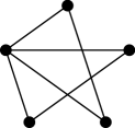
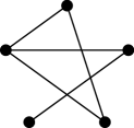
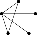
Figure 1: $K_{3}\star K_{3}$ (left), $G_{1}$ (middle) and $G_{2}$ (right)

Example 4.10.

We consider $K_{3}\star P_{3}$, where $P_{3}$ is the path on three vertices. There are two non-isomorphic star products in this case, say, $G_{1}$ and $G_{2}$ as shown in Figure 1. It is known that $\mathrm{QEC}(K_{3})=-1$ and $\mathrm{QEC}(P_{3})=-2/3$. Inserting $Q_{1}=-1$, $Q_{2}=-2/3$, $n_{1}+1=n_{2}+1=3$ into (4.22), we have

$$Q_{12}=\frac{-15+\sqrt{105}}{10}=-\frac{12}{15+\sqrt{105}}\approx-0.4753.$$

On the other hand, it follows by a direct calculation (see also [15, Sect. 5.2, No. 4 and No. 7]) that

$$\mathrm{QEC}(G_{1})=-\frac{6}{6+\sqrt{21}}\approx-0.5670,\qquad\mathrm{QEC}(G_{2})=-\frac{12}{15+\sqrt{105}}\,.$$

Thus, we obtain an interesting contrast:

$$\max\{Q_{1},Q_{2}\}<\mathrm{QEC}(G_{1})<Q_{12}<0,$$

$$\max\{Q_{1},Q_{2}\}<\mathrm{QEC}(G_{2})=Q_{12}<0.$$

Example 4.11.

It is known that $\mathrm{QEC}(K_{2})=-1$ and $\mathrm{QEC}(C_{4})=0$, where $C_{4}$ is the cycle on four vertices. It follows from Theorem 4.4 that $\mathrm{QEC}(K_{2}\star C_{4})=0$. On the other had, inserting $Q_{1}=-1$, $Q_{2}=0$, $n_{1}+1=2$ and $n_{2}+1=4$ into (4.22), we have $Q_{12}=0$. Thus we have

$$\max\{Q_{1},Q_{2}\}=\mathrm{QEC}(K_{2}\star C_{4})=Q_{12}=0.$$

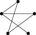
Figure 2: $K_{2}\star C_{4}$

Along with the above observation, a natural question arises to determine the extremal classes of star products $G_{1}\star G_{2}$ such that

$$\mathrm{QEC}(G_{1}\star G_{2})=Q_{12}$$

and

$$\mathrm{QEC}(G_{1}\star G_{2})=\max\{Q_{1},Q_{2}\}.$$

Remind that the star product depends also on the choice of distinguished vertices $o_{1}$ and $o_{2}$, as is illustrated in Example 4.10.

5 Infinite graphs

5.1 A limit formula

Proposition 5.1.

Let $G=(V,E)$ be a connected graph. Let $H_{n}=(W_{n},F_{n})$ be a sequence of connected subgraphs of $G$ such that $W_{1}\subset W_{2}\subset\dotsb$ and $V=\bigcup_{n=1}^{\infty}W_{n}$. If each $H_{n}$ is isometrically embedded in $G$, we have

$$\mathrm{QEC}(G)=\lim_{n\rightarrow\infty}\mathrm{QEC}(H_{n}).$$ (5.1)

Proof.

Let $D$ denote the distance matrix of $G$. By definition, for any $\epsilon>0$ there exists $f\in C_{0}(V)$ such that $\langle f,f\rangle=1$, $\langle\bm{1},f\rangle=0$ and $\langle f,Df\rangle\geq\mathrm{QEC}(G)-\epsilon$. By assumption we may choose $n_{0}$ such that $f(x)=0$ outside of $W_{n}$ for all $n\geq n_{0}$. Then $\mathrm{QEC}(H_{n})\geq\langle f,Df\rangle$ for all $n\geq n_{0}$ and we have

$$\mathrm{QEC}(G)-\epsilon\leq\mathrm{QEC}(H_{n}),\qquad n\geq n_{0}.$$

On the other hand, it follows from Proposition 4.1 that

$$\mathrm{QEC}(H_{n})\leq\mathrm{QEC}(G)$$

Consequently, (5.1) holds. ∎

Proposition 5.2.

Any (finite or infinite) tree is of QE class.

Proof.

For any tree we may choose a sequence of finite subtrees of which the union covers the whole tree. Note that any subtree of a tree is isometrically embedded. Then, in view of Proposition 5.1 it is sufficient to show that every finite tree is of QE class. More precisely, for a finite tree $G=(V,E)$ on $|V|\geq 3$ vertices we have

$$\mathrm{QEC}(G)<-\frac{1}{|V|-1}\,.$$ (5.2)

In fact, a tree on $n$ vertices is represented as $G=G_{1}\star\dots\star G_{n-1}$, where each $G_{j}$ is isomorphic to $K_{2}$. Note that $Q_{j}=\mathrm{QEC}(G_{j})=\mathrm{QEC}(K_{2})=-1$. Then by Corollary 4.6 we obtain

$$\mathrm{QEC}(G)=\mathrm{QEC}(G_{1}\star\dots\star G_{n-1})<\left(\frac{1}{Q_{1}}+\dots+\frac{1}{Q_{n-1}}\right)^{-1}=-\frac{1}{n-1}\,,$$

as desired. ∎

The above result is a reproduction of Haagerup [6]. The estimate (5.2) is far from best possible. It is an interesting question to determine the QE constant of a tree.

Proposition 5.3.

Let $K_{\infty}$ be the infinite complete graph, that is, the graph on a countably infinite set such that any pair of distinct vertices are connected by an edge. Then $\mathrm{QEC}(K_{\infty})=-1$.

Proof.

Every finite subgraph of $K_{\infty}$ is of the form $K_{n}$ and $\mathrm{QEC}(K_{n})=-1$. Now we apply Proposition 5.1. ∎

5.2 The path graphs $P_{n}$

For $n\geq 1$ let $P_{n}$ be the path graph on the vertex set $V=\{0,1,2,\dots,n-1\}$ and edge set $E=\{\{0,1\},\{1,2\},\dots,\{n-2,n-1\}\}$. Let $D=[d(i,j)]$ be the distance matrix as usual. Note that $d(i,j)=|i-j|$ for $i,j\in V$. We start with the following

Proposition 5.4.

For $n\geq 1$ let $c_{n}$ be the maximal number $c$ such that the $n\times n$ matrix

$$\left[2\min\{i,j\}-c-c\cdot\delta_{ij}\right]_{i,j=1}^{n}$$ (5.3)

is positive definite. Then $\mathrm{QEC}(P_{n+1})=-c_{n}$.

Proof.

Suppose $f\in C(V)$ satisfies $\langle\bm{1},f\rangle=0$. Then we have

$$\langle f,Df\rangle =\sum_{i,j=0}^{n}|i-j|f(i)f(j)$$

$$=\sum_{i=1}^{n}if(i)f(0)+\sum_{j=1}^{n}jf(0)f(j)+\sum_{i,j=1}^{n}|i-j|f(i)f(j).$$ (5.4)

For $1\leq i\leq n$ we set $x_{i}=f(i)$. Since $f(0)=-x_{1}-\dots-x_{n}$, (5.4) becomes

$$\langle f,Df\rangle=\sum_{i,j=1}^{n}(-i-j+|i-j|)x_{i}x_{j}=-\sum_{i,j=1}^{n}2\min\{i,j\}\,x_{i}x_{j}$$ (5.5)

On the other hand, we have

$$\langle f,f\rangle=\sum_{i=0}^{n}f(i)^{2}=\left(\sum_{i=1}^{n}x_{i}\right)^{2}+\sum_{i=1}^{n}x_{i}^{2}=\sum_{i,j=1}^{n}(1+\delta_{ij})x_{i}x_{j}.$$ (5.6)

The QE constant is the minimal constant $Q\in\mathbb{R}$ such that $\langle f,Df\rangle\leq Q\langle f,f\rangle$ for all $f\in C(V)$ with $\langle\bm{1},f\rangle=0$, or using (5.5) and (5.6),

$$-\sum_{i,j=1}^{n}2\min\{i,j\}x_{i}x_{j}\leq Q\sum_{i,j=1}^{n}(1+\delta_{ij})x_{i}x_{j}$$

holds for every choice of $x_{1},\dots,x_{n}\in\mathbb{R}$, In other words, $Q$ coincides with $-c$, where $c\in\mathbb{R}$ is the maximal constant such that

$$\sum_{i,j=1}^{n}(2\min\{i,j\}-c(1+\delta_{ij}))x_{i}x_{j}\geq 0$$

for every choice of $x_{1},\dots,x_{n}\in\mathbb{R}$. This completes the proof. ∎

By direct application of Proposition 5.4 we obtain

$$-\mathrm{QEC}(P_{2}) =1,$$

$$-\mathrm{QEC}(P_{3}) =2/3,$$

$$-\mathrm{QEC}(P_{4}) =2-\sqrt{2}=0.585786\ldots,$$

$$-\mathrm{QEC}(P_{5}) =(5-\sqrt{5})/5=0.552786\ldots,$$

$$-\mathrm{QEC}(P_{6}) =4-2\sqrt{3}=0.535898\ldots,$$

$$-\mathrm{QEC}(P_{7}) =0.526048\ldots,$$

$$-\mathrm{QEC}(P_{8}) =4+2\sqrt{2}-\sqrt{20+14\sqrt{2}}=0.519783\ldots,$$

$$-\mathrm{QEC}(P_{9}) =0.515546\ldots,$$

$$-\mathrm{QEC}(P_{10}) =6+2\sqrt{5}-\sqrt{50+22\sqrt{5}}=0.512543\ldots.$$

The numbers $-\mathrm{QEC}(P_{7})$ and $-\mathrm{QEC}(P_{9})$ are the smallest real roots of the cubic equations

$$7c^{3}-28c^{2}+28c-8=0,\qquad 3c^{3}-18c^{2}+24c-8=0,$$

respectively.

Now define a family of matrices: $A_{n}=\left[4\min\{i,j\}-1-\delta_{ij}\right]_{i,j=1}^{n}$, where $1\leq n\leq\infty$. In particular

$$A_{\infty}=\begin{bmatrix}2&3&3&3&3&\cdots\\ 3&6&7&7&7&\cdots\\ 3&7&10&11&11&\cdots\\ 3&7&11&14&15&\cdots\\ 3&7&11&15&18&\cdots\\ \vdots&\vdots&\vdots&\vdots&\vdots&\ddots\end{bmatrix}.$$

Proposition 5.5.

For $n\geq 1$,

$$\det A_{n}=n+1.$$

Consequently, $A_{\infty}$ is positive definite as well as $A_{n}$ for all $n\geq 1$.

Proof.

We are going to prove a slightly more general statement. For $n\geq 1$ and $u\in\mathbb{R}$ we define an auxiliary matrix $A_{n}(u)=[u_{ij}]_{i,j=1}^{n}$, where

$$u_{ij}=\begin{cases}4\min\{i,j\}-1-\delta_{ij}\,,&(i,j)\neq(n,n),\\ u,&(i,j)=(n,n).\end{cases}$$

Then $A_{n}=A_{n}(4n-2)$. We will prove that

$$\det A_{n}(u)=nu-(n-1)(4n+1).$$ (5.7)

This is true for $n=1$. Assume that (5.7) holds for $n-1$. Let $\bm{k}_{j}$ denote the $j$th column of $A_{n}(u)$. Then

$$\det A_{n}(u)=\det[\bm{k}_{1}\,,\dots,\bm{k}_{n}]=\det[\bm{k}_{1}\,,\dots,\bm{k}_{n-1}\,,\bm{k}_{n}-\bm{k}_{n-1}].$$

Now we observe that

$$\bm{k}_{n}-\bm{k}_{n-1}=[0,\dots,0,1,u-4n+5]^{\mathrm{T}},$$

so expanding the determinant over the last column and applying the inductive assumption we get

$$\det A_{n}(u) =(u-4n+5)\det A_{n-1}-\det A_{n-1}(4n-5)$$

$$=(u-4n+5)n-(n-1)(4n-5)+(n-2)(4n-3)$$

$$=nu-(n-1)(4n+1),$$

hence (5.7) holds for $n$. ∎

Theorem 5.6.

For $n\geq 2$ we have

$$-\frac{2n^{4}+20n^{2}-7+15(-1)^{n}}{4n^{4}-4+15n+15n(-1)^{n}}\leq\mathrm{QEC}(P_{n})\leq-\frac{1}{2}.$$ (5.8)

Proof.

For the right half of (5.8) it suffices to note that for $c=1/2$ the matrix $A_{n}$ is a multiple by $2$ of the matrix given by (5.3).

We will prove the left half of (5.8). Suppose that the matrix

$$\left[2\min\{i,j\}-c-c\cdot\delta_{ij}\right]_{i,j=1}^{n-1}$$

is positive definite. Then for $a_{i}^{(n)}=i(n-i)(-1)^{i}$ we have

$$\sum_{i,j=1}^{n-1}\left(2\min\{i,j\}-c-c\cdot\delta_{ij}\right)a_{i}^{(n)}a_{j}^{(n)}\geq 0.$$ (5.9)

The above sum is calculated with the help of Lemma 6.1 in the Appendix as follows:

$$\sum_{i,j=1}^{n-1}\left(2\min\{i,j\}-c-c\cdot\delta_{ij}\right)a_{i}^{(n)}a_{j}^{(n)}$$

$$=2\sum_{i,j=1}^{n-1}\min\{i,j\}\,i(n-i)j(n-j)(-1)^{i+j}$$

$$\qquad-c\sum_{i,j=1}^{n-1}i(n-i)j(n-j)(-1)^{i+j}-c\sum_{i=1}^{n-1}i^{2}(n-i)^{2}$$

$$=\frac{n}{120}\left\{2n^{4}+20n^{2}-7+15(-1)^{n}\right\}-\frac{c}{8}\left\{1+(-1)^{n}\right\}n^{2}-c\,\frac{n^{5}-n}{30}.$$

Then, (5.9) yields

$$c\leq\frac{2n^{4}+20n^{2}-7+15(-1)^{n}}{4n^{4}-4+15n+15n(-1)^{n}}\,,$$

which, in view of Proposition 5.4, proves (5.8). ∎

Let $\mathbb{Z}$ be the one-dimensional integer lattice, i.e., the two-sided infinite path on the integers, and $\mathbb{Z}_{+}$ be the one-sided infinite path on $\{0,1,2,\dots\}$.

Theorem 5.7.

$\mathrm{QEC}(\mathbb{Z}_{+})=\mathrm{QEC}(\mathbb{Z})=-\dfrac{1}{2}$ .

Proof.

Every finite connected subgraph of $\mathbb{Z}_{+}$ and $\mathbb{Z}$ is of the form $P_{n}$ and $n$ can be arbitrarily large. Therefore our statement is a consequence of Theorem 5.6 and Proposition 5.1. ∎

6 Appendix

6.1 Some combinatorial identities

In this part we are going to prove three identities which were used in the proof of Theorem 5.6.

Lemma 6.1.

For $n\geq 1$ we have

$$\sum_{i,j=1}^{n}\min\{i,j\}\,i(n-j)j(n-j)(-1)^{i+j}=\frac{n}{240}\left\{2n^{4}+20n^{2}-7+15(-1)^{n}\right\},$$ (6.1)

$$\sum_{i,j=1}^{n}i(n-i)j(n-j)(-1)^{i+j}=\frac{1}{8}\left(1+(-1)^{n}\right)n^{2},$$ (6.2)

$$\sum_{i=1}^{n}i^{2}(n-i)^{2}=\frac{n^{5}-n}{30}\,.$$ (6.3)

Proof.

For $n=0$ the identities remain true understanding that the left-hand sides are zero. The above three identities are used in the proof of Theorem 5.6. For the proofs we will apply well-known formulas for the sums:

$$\sum_{i=1}^{n}i =\frac{1}{2}n(n+1), \sum_{i=1}^{n}i^{2} =\frac{1}{6}n(n+1)(2n+1),$$

$$\sum_{i=1}^{n}i^{3} =\frac{1}{4}n^{2}(n+1)^{2}, \sum_{i=1}^{n}i^{4} =\frac{1}{30}(n+1)(2n+1)(3n^{2}+3n-1),$$

and also the following elementary identities:

$$\sum_{i=1}^{n}i(-1)^{i} =\frac{1}{4}\left(2n(-1)^{n}+(-1)^{n}-1\right),$$

$$\sum_{i=1}^{n}i^{2}(-1)^{i} =\frac{1}{2}n(n+1)(-1)^{n},$$

$$\sum_{i=1}^{n}i^{3}(-1)^{i} =\frac{1}{8}\left\{4n^{3}(-1)^{n}+6n^{2}(-1)^{n}-(-1)^{j}+1\right\}.$$

Now we prove (6.1). Put

$$A_{j} =\sum_{i=1}^{j}i^{2}(n-i)j(n-j)(-1)^{i+j},$$

$$B_{j} =\sum_{i=j+1}^{n}i(n-i)j^{2}(n-j)(-1)^{i+j}.$$

By elementary calculations we find that

$$A_{j} =\frac{j(n-j)}{8}\left\{4j^{2}n+4jn-4j^{3}-6j^{2}+1-(-1)^{j}\right\},$$

$$B_{j} =\frac{j^{2}(n-j)}{4}\left\{2j^{2}+2j-n-2jn-(-1)^{j+n}n\right\}.$$

Then we have

$$A_{j}+B_{j} =\sum_{i=1}^{n}\min\{i,j\}\,i(n-i)j(n-j)(-1)^{i+j}$$

$$=\frac{1}{8}j(n-j)\left\{2jn-2j^{2}+1-2(-1)^{j+n}jn-(-1)^{j}\right\}.$$

Summing up both sides over $j=1,2,\dots,n$, we get (6.1).

Relation (6.2) follows from

$$\sum_{i,j=1}^{n}i(n-i)j(n-j)(-1)^{i+j} =\left(\sum_{i=1}^{n}i(n-i)(-1)^{i}\right)^{2}$$

$$=\left(\frac{-\left(1+(-1)^{n}\right)n}{4}\right)^{2}=\frac{\left(1+(-1)^{n}\right)n^{2}}{8}.$$

Relation (6.3) can be shown in a similar manner. ∎

6.2 A new integer sequence

For $n\geq 0$ let $a_{n}$ be the number given by (6.1), i.e.,

$$a_{n} =\sum_{i,j=1}^{n}\min\{i,j\}\,i(n-j)j(n-j)(-1)^{i+j}$$

$$=\frac{n}{240}\left\{2n^{4}+20n^{2}-7+15(-1)^{n}\right\}.$$ (6.4)

Then the sequence $\{a_{n}\}_{n=0}^{\infty}$ begins with

$$0,0,1,4,14,36,83,168,316,552,917,1452,2218,3276,4711,6608,\dots$$

and is absent in OEIS [16]. Applying formula

$$\sum_{n=1}^{\infty}n^{N}z^{n}=\frac{zP_{N}(z)}{(1-z)^{N+1}},$$

where $P_{N}(z)$ are the classical Eulerian polynomials, we can compute the generating function:

$$\sum_{n=0}^{\infty}a_{n}z^{n}=\frac{z^{2}(1+z^{2})^{2}}{(1+z)^{2}(1-z)^{6}}.$$ (6.5)

Denote the ceiling of $n^{2}/2$ by $b_{n}=\lceil n^{2}/2\rceil$. This sequence appears in OEIS as A000982. Now we observe that $a_{n}$ is the convolution of the sequence $b_{n}$ with itself.

Proposition 6.2.

For every $n\geq 0$ we have $a_{n}=\sum_{k=0}^{n}b_{k}b_{n-k}$.

Proof.

The generating function for $a_{n}$ is the square of

$$\frac{z(1+z^{2})}{(1+z)(1-z)^{3}},$$

which is the generating function for $b_{n}$, see entry A000982 in OEIS. ∎

References

- [1] M. Aouchiche and P. Hansen: Distance spectra of graphs: a survey, Linear Algebra Appl. 458 (2014), 301–386.
- [2] R. Balaji and R. B. Bapat: On Euclidean distance matrices, Linear Algebra Appl. 424 (2007), 108–117.
- [3] R. B. Bapat: “Graphs and Matrices,” Springer, Hindustan Book Agency, New Delhi, 2010.
- [4] M. Bożejko, T. Januszkiewicz and R. J. Spatzier: Infinite Coxeter groups do not have Kazhdan’s property, J. Operator Theory 19 (1988), 63–67.
- [5] M. Bożejko: Positive-definite kernels, length functions on groups and noncommutative von Neumann inequality, Studia Math. 95 (1989), 107–118.
- [6] U. Haagerup: An example of a nonnuclear C∗-algebra which has the metric approximation property, Invent. Math. 50 (1979), 279–293.
- [7] A. Hora and N. Obata: “Quantum Probability and Spectral Analysis of Graphs,” Springer, 2007.
- [8] G. Jaklič and J. Modic: On properties of cell matrices. Appl. Math. Comput. 216 (2010), 2016–2023.
- [9] G. Jaklič and J. Modic: On Euclidean distance matrices of graphs, Electron. J. Linear Algebra 26 (2013), 574–589.
- [10] G. Jaklič and J. Modic: Euclidean graph distance matrices of generalizations of the star graph, Appl. Math. Comput. 230 (2014), 650–663.
- [11] L. Liberti, G. Lavor, N. Maculan and A. Mucherino: Euclidean distance geometry and applications, SIAM Rev. 56 (2014), 3–69.
- [12] W. Młotkowski: Positive and negative definite kernels on trees, in “Harmonic Analysis and Discrete Potential Theory”, pp. 107–110, Plenum Press, 1992.
- [13] N. Obata: Positive Q-matrices of graphs, Studia Math. 179 (2007), 81–97.
- [14] N. Obata: Markov product of positive definite kernels and applications to Q-matrices of graph products, Colloq. Math. 122 (2011), 177–184.
- [15] N. Obata and A. Y. Zakiyyah: Distance matrices and quadratic embedding of graphs, preprint, 2017.
- [16] The On-Line Encyclopedia of Integer Sequences, https://oeis.org/
- [17] I. J. Schoenberg: Remarks to Maurice Fréchet’s article “Sur la définition axiomatique d’une classe d’espace distanciś vectoriellement applicable sur l’espace de Hilbert”, Ann. of Math. 36 (1935), 724–732.
- [18] I. J. Schoenberg: Metric spaces and positive definite functions, Trans. Amer. Math. Soc. 44 (1938), 522–536.
- [19] G. Young and A. S. Householder: Discussion of a set of points in terms of their mutual distances, Psychometrika 3 (1938), 1–22.