We study charge transport and fluctuations of the (3+1)-dimensional massive free Dirac theory. In particular, we focus on the steady state that emerges following a local quench whereby two independently thermalized halves of the system are connected and let to evolve unitarily for a long time. Based on the two-time von Neumann measurement statistics and exact computations, the scaled cumulant generating function associated with the charge transport is derived. We find that it can be written as a generalization of Levitov-Lesovik formula to the case in three spatial dimensions. In the massless case, we note that only the first four scaled cumulants are nonzero. Our results provide also a direct confirmation for the validity of the extended fluctuation relation in higher dimensions. An application of our approach to Lifshitz fermions is also briefly discussed.

1 Introduction

Our understanding on transport phenomena in quantum many-body systems has been significantly advanced by fruitful interactions between theory and experiment over the past decades. There are many possible situations to study transport phenomena, and one of the simplest protocols would be a local quench where a non-equilibrium steady state (NESS) is generated upon gluing two systems, which are initially prepared at different parameters (say chemical potentials or temperatures). This so-called partitioning protocol has gained a surge of interest in recent years [1, 2] leading to studies on a variety of models in the protocol, from one-dimensional integrable systems to higher dimensional quantum critical systems [3, 4, 5, 6, 7, 8, 9, 10, 11, 12]. That being said, it is important to note that these studies have focused mainly on one-dimensional systems due to the abundance of available analytical approaches and simulability by powerful numerical methods such as tDMRG in one dimension. This is in stark contrast with the case in higher dimensions where relatively less is known. This case also applies to the study of charge fluctuation (a.k.a. full counting statistics) in which a significant amount of works have been done on one-dimensional electron (impurity) systems [13, 14, 15, 16, 17, 18, 19], initiated by a seminal work by Levitov and Lesovik [20, 21] in 90s. In view of these situations, it is urgent to reinforce our understanding on the non-equilibrium dynamics and fluctuations in higher dimensions. In this work, we present a first detailed analysis on the full counting statistics in the (3+1)-D Dirac theory using the partitioning protocol. On the experimental side, for the last decade, a surprising ubiquity of Dirac fermions in nature, such as graphene [22] and Dirac semimetal [23] has been realized. It is therefore paramount to understand its transport nature in one of the simplest and cleanest situations which could serve as a benchmark.

It is worth recalling what has been done concerning the studies on non-equilibrium transport in higher dimensions. Being initiated by the work [5], studies on NESS in higher dimensions have been addressed by AdS/CFT correspondence (for quantum critical systems) [5], exact computations (for free models) [6, 7], and hydrodynamics [8, 9], which, in general, plays a pivotal role in studying transport phenomena. In particular, while the quantities of primary interest are the space-time profiles of the local density and current in NESS, the fluctuation in energy transport and the approach of observables towards NESS in the higher-D Klein-Gordon model were also studied in [7] by making use of powerful free field techniques. The techniques developed there will be intensively exploited in this paper as well.

The present paper deals with yet another representative free model, the (3+1)-D free Dirac model, and discusses the charge fluctuation in the NESS generated by a local quench. Since the model possesses two charged particles, Dirac fermions and anti-Dirac fermions, we expect that there occurs a $U(1)$-charge flow when two systems with different global parameters are put in contact. A local quench we consider can be regarded as a simpler version of the protocol used in the study of full counting statistics: the total Hamiltonian that does time-evolution now is without impurities, thus particles are transferred without reflection at the junction (i.e. the transmission coefficient is simply 1). A typical quantity that encodes all the information about the charge fluctuation is the scaled cumulant generating function (SCGF), which is a generating function for the probability distribution of the transferred $U(1)$-charge across the contact surface for the duration of large time $t\to\infty$ (the infinite system size limit $L\to\infty$ is taken first so that the propagation front does not reach the boundary). There are two situations for which we can compute the SCGF. One is to prepare the initial state $\rho_{\rm L}\otimes\rho_{\rm R}$, where $\rho_{\rm L}$ and $\rho_{\rm R}$ are the density operators of the left and right baths, at $t=0$ and focus on the charges transferred between $t=0$ and $t\to\infty$. In this situation, the counted charges are not necessarily carried by the NESS as the NESS is reached only at large time. Another case is where the initial state is prepared at $t=t_{0}\to-\infty$ so that at $t=0$ the NESS emerges across the interface. The system is then fully in the NESS between time $t=0$ and $t\to\infty$ during which the transferred charges are counted, and this is the scenario we shall be interested in. In order to assess the SCGF, we first derive the stationary density operator that describes NESS. This allows us to explicitly evaluate the SCGF based on the two-time von Neumann measurement statistics where computations are carried out by free field techniques [7]. It is found that the so-obtained SCGF is nothing but a straightforward generalization of the Levitov-Lesovik formula for (3+1)-D Dirac theory, implying the universality of the formula regardless of the dimensionality. Interestingly, the SCGF has a particularly simple form in the massless limit, and it turns out that the cumulants exist only up to fourth order. We also check the validity of the extended fluctuation theorem (EFR) proposed in [24] for the SCGF, which is expected to hold in free theories and 2D conformal field theories.

2 Non-equilibrium steady-state of the model

2.1 The Dirac model

In order to introduce our notation, we briefly recall the canonical quantization of the Dirac model. The Hamiltonian of the relativistic Dirac theory is given by

$$H=\int d^{3}x:\psi^{\dagger}(-\mathrm{i}\gamma^{0}\vec{\gamma}\cdot\vec{\nabla}+m\gamma^{0})\psi:,$$ (1)

where the fermionic field operators are defined as

$$\psi(\vec{x},t) =\int Dp\sum_{s}(a_{\vec{p}}^{s}u^{s}(p)e^{-\mathrm{i}p\cdot x}+b_{\vec{p}}^{s\dagger}v^{s}(p)e^{\mathrm{i}p\cdot x})$$ (2)

$$\overline{\psi}(\vec{x},t) =\int Dp\sum_{s}(b_{\vec{p}}^{s}\bar{v}^{s}(p)e^{-\mathrm{i}p\cdot x}+a_{\vec{p}}^{s\dagger}\bar{u}^{s}(p)e^{\mathrm{i}p\cdot x}),$$ (3)

with $p\cdot x=p^{\mu}x_{\mu}$ ($g_{\mu\nu}=\mathrm{diag}(1,-1,-1,-1)$) and $Dp=d^{3}p/(2\pi)^{3}\sqrt{2E_{\vec{p}}}$. Furthermore, spinors $u^{s}(p)$ and $v^{s}(p)$ are expressed as

$$u^{s}(p)=\left(\begin{array}[]{c}\sqrt{p\cdot\sigma}\xi^{s}\\ \sqrt{p\cdot\bar{\sigma}}\xi^{s}\end{array}\right),\ \ v^{s}(p)=\left(\begin{array}[]{c}\sqrt{p\cdot\sigma}\eta^{s}\\ -\sqrt{p\cdot\bar{\sigma}}\eta^{s}\end{array}\right),$$ (4)

where $\xi^{s}$ and $\eta^{s}$ are two different bases of two-component spinors, and $\sigma^{\mu}=(\hat{1},\vec{\sigma})$ and $\bar{\sigma}^{\mu}=(\hat{1},-\vec{\sigma})$. The creation and annihilation operators satisfy the anti-commutation relation rules

$$\{a_{\vec{p}}^{s},a_{\vec{q}}^{r\dagger}\}=\{b_{\vec{p}}^{s},b_{\vec{q}}^{r\dagger}\}=\hat{\delta}^{(3)}(\vec{p}-\vec{q})\delta^{rs}$$ (5)

where we defined $\hat{\delta}^{(3)}(\vec{p}-\vec{q})=(2\pi)^{3}\delta^{(3)}(\vec{p}-\vec{q})$, and with all other anti-commutators being zero. This implies equal-time anti-commutation relations

$$\{\psi_{a}(\vec{x}),\psi_{b}^{\dagger}(\vec{y})\}=\delta^{(3)}(\vec{x}-\vec{y})\delta_{ab},\{\psi_{a}(\vec{x}),\psi_{b}(\vec{y})\}=\{\psi_{a}^{\dagger}(\vec{x}),\psi_{b}^{\dagger}(\vec{y})\}=0.$$ (6)

The initial density matrix is simply defined as a (tensor) product of sub-density matrices representing subsystems in thermal equilibrium with different temperatures and chemical potentials:

$$\rho_{\mathrm{th}}=\exp[-\beta_{\mathrm{L}}(H_{\mathrm{L}}-\mu_{\mathrm{L}}Q_{\mathrm{L}})-\beta_{\mathrm{R}}(H_{\mathrm{R}}-\mu_{\mathrm{R}}Q_{\mathrm{R}})],$$ (7)

where $H_{\mathrm{L},\mathrm{R}}$ and $Q_{\mathrm{L},\mathrm{R}}$ are Hamiltonians and $U(1)$ charges for subsystems defined as

$$H_{\mathrm{L},\mathrm{R}} =\int_{x_{1}\lessgtr 0}d^{3}x:\psi^{\dagger}(-\mathrm{i}\gamma^{0}\vec{\gamma}\cdot\vec{\nabla}+m\gamma^{0})\psi:$$ (8)

$$Q_{\mathrm{L},\mathrm{R}} =\int_{x_{1}\lessgtr 0}d^{3}x\psi^{\dagger}(\vec{x})\psi(\vec{x}),$$ (9)

and with $\mu_{\mathrm{L},\mathrm{R}}$ being chemical potentials for semi-halves. The total $U(1)$ charge can be expressed in terms of creation and annihilation operators

$$Q=\int\frac{d^{3}p}{(2\pi)^{3}}\sum_{s}(a_{\vec{p}}^{s\dagger}a_{\vec{p}}^{s}-b_{\vec{p}}^{s\dagger}b_{\vec{p}}^{s}).$$ (10)

2.2 NESS density operator

In order to analyze the charge fluctuation (large deviation) of the Dirac theory, we need an explicit expression of the NESS density operator $\rho_{\rm s}$, which is defined by, for a generic field $\mathcal{O}$,

$$\mathrm{Tr}(\mathfrak{n}[\rho_{\rm s}]\mathcal{O})=\lim_{t\to\infty}\mathrm{Tr}(\mathfrak{n}[\rho_{\rm th}]e^{\mathrm{i}Ht}\mathcal{O}e^{-\mathrm{i}Ht}),$$ (11)

where $\mathfrak{n}[\rho]=\rho/\mathrm{Tr}\rho$ for $\rho=\rho_{\rm s},\rho_{\rm th}$. In what follows, we will show that the explicit form of $\rho_{\rm s}$ reads

$$\rho_{\mathrm{s}} =\exp[-\beta_{\mathrm{L}}(H_{\mathrm{L}}^{+}-\mu_{\mathrm{L}}Q_{\mathrm{L}}^{+})-\beta_{\mathrm{R}}(H_{\mathrm{R}}^{+}-\mu_{\mathrm{R}}Q_{\mathrm{R}}^{+})]$$

$$=\exp\Bigl{[}-\int\frac{d^{3}p}{(2\pi)^{3}}\sum_{s}(V_{+}(\vec{p})a_{\vec{p}}^{s\dagger}a_{\vec{p}}^{s}+V_{-}(\vec{p})b_{\vec{p}}^{s\dagger}b_{\vec{p}}^{s})\Bigr{]},$$ (12)

with

$$H_{\mathrm{L},\mathrm{R}}^{+} =\int_{p^{1}\gtrless 0}\frac{d^{3}p}{(2\pi)^{3}}E_{{\bf p}}\sum_{s}(a_{\vec{p}}^{s\dagger}a_{\vec{p}}^{s}+b_{\vec{p}}^{s\dagger}b_{\vec{p}}^{s})$$ (13)

$$Q_{\mathrm{L},\mathrm{R}}^{+} =\int_{p^{1}\gtrless 0}\frac{d^{3}p}{(2\pi)^{3}}\sum_{s}(a_{\vec{p}}^{s\dagger}a_{\vec{p}}^{s}-b_{\vec{p}}^{s\dagger}b_{\vec{p}}^{s}),$$ (14)

and where

$$V_{+}(\vec{p})=\begin{cases}\beta_{\mathrm{L}}(E_{\vec{p}}-\mu_{\mathrm{L}})&\text{$p^{1}>0$}\\ \beta_{\mathrm{R}}(E_{\vec{p}}-\mu_{\mathrm{R}})&\text{$p^{1}<0$}\end{cases},\ \ V_{-}(\vec{p})=\begin{cases}\beta_{\mathrm{L}}(E_{\vec{p}}+\mu_{\mathrm{L}})&\text{$p^{1}>0$}\\ \beta_{\mathrm{R}}(E_{\vec{p}}+\mu_{\mathrm{R}})&\text{$p^{1}<0$}\end{cases}.$$ (15)

For later convenience, we note that the NESS density operator $\rho_{\rm s}$ satisfies the following contraction relations

$$\begin{split}\mathrm{Tr}(\mathfrak{n}[\rho_{\mathrm{s}}]a_{\vec{p}}^{s\dagger}a_{\vec{q}}^{r})&=\frac{\hat{\delta}^{(3)}(\vec{p}-\vec{q})\delta^{rs}}{1+e^{V_{+}(\vec{p})}},\quad\mathrm{Tr}(\mathfrak{n}[\rho_{\mathrm{s}}]b_{\vec{p}}^{s\dagger}b_{\vec{q}}^{r})=\frac{\hat{\delta}^{(3)}(\vec{p}-\vec{q})\delta^{rs}}{1+e^{V_{-}(\vec{p})}}\\ \mathrm{Tr}(\mathfrak{n}[\rho_{\mathrm{s}}]a_{\vec{p}}^{s}a_{\vec{q}}^{r\dagger})&=\frac{\hat{\delta}^{(3)}(\vec{p}-\vec{q})\delta^{rs}}{1+e^{-V_{+}(\vec{p})}},\quad\mathrm{Tr}(\mathfrak{n}[\rho_{\mathrm{s}}]b_{\vec{p}}^{s}b_{\vec{q}}^{r\dagger})=\frac{\hat{\delta}^{(3)}(\vec{p}-\vec{q})\delta^{rs}}{1+e^{-V_{-}(\vec{p})}}.\end{split}$$ (16)

The following derivation will closely parallel the argument employed in [7]. First let us introduce the “B-representation” of the fundamental fields. Recall that the representation (2) with (5), which we call the “A-representation” as in [7], diagonalizes the total Hamiltonian (1). The B-representation instead diagonalizes Hamiltonians of each half (8). With a natural choice of a boundary condition $\psi_{\rm B}(x^{1}=0,\tilde{x})=0$, where $\tilde{x}=(x^{2},x^{3})$, the Dirac fields in the B-representation read

$$\psi_{\rm B}(\vec{x}) =\int Dp\sum_{s}(A_{\vec{p}}^{s}u^{s}(p)e^{-i\vec{p}\cdot\vec{x}}+B_{\vec{p}}^{s\dagger}v^{s}(p)e^{ip\cdot x})(\vartheta(p^{1}x^{1})-\vartheta(-p^{1}x^{1}))$$ (17)

$$\overline{\psi}_{\rm B}(\vec{x}) =\int Dp\sum_{s}(B_{\vec{p}}^{s}\bar{v}^{s}(p)e^{-ip\cdot x}+A_{\vec{p}}^{s\dagger}\bar{u}^{s}(p)e^{ip\cdot x})(\vartheta(p^{1}x^{1})-\vartheta(-p^{1}x^{1})),$$ (18)

where $A_{\vec{p}}^{s},A_{\vec{p}}^{s\dagger},B_{\vec{p}}^{s}$, and $B_{\vec{p}}^{s\dagger}$ satisfy the same anti-commutation relation (5) and

$$H_{\mathrm{L},\mathrm{R}} =\int_{p^{1}\gtrless 0}\frac{d^{3}p}{(2\pi)^{3}}E_{{\bf p}}\sum_{s}(A_{\vec{p}}^{s\dagger}A_{\vec{p}}^{s}+B_{\vec{p}}^{s\dagger}B_{\vec{p}}^{s})$$ (19)

$$Q_{\mathrm{L},\mathrm{R}} =\int_{p^{1}\gtrless 0}\frac{d^{3}p}{(2\pi)^{3}}\sum_{s}(A_{\vec{p}}^{s\dagger}A_{\vec{p}}^{s}-B_{\vec{p}}^{s\dagger}B_{\vec{p}}^{s}).$$ (20)

This implies the following contraction rules

$$\begin{split}\mathrm{Tr}(\mathfrak{n}[\rho_{\rm th}]A_{\vec{p}}^{s\dagger}A_{\vec{q}}^{r})&=\frac{\hat{\delta}^{(3)}(\vec{p}-\vec{q})\delta^{rs}}{1+e^{V_{+}(\vec{p})}},\quad\mathrm{Tr}(\mathfrak{n}[\rho_{\rm th}]B_{\vec{p}}^{s\dagger}B_{\vec{q}}^{r})=\frac{\hat{\delta}^{(3)}(\vec{p}-\vec{q})\delta^{rs}}{1+e^{V_{-}(\vec{p})}}\\ \mathrm{Tr}(\mathfrak{n}[\rho_{\rm th}]A_{\vec{p}}^{s}A_{\vec{q}}^{r\dagger})&=\frac{\hat{\delta}^{(3)}(\vec{p}-\vec{q})\delta^{rs}}{1+e^{-V_{+}(\vec{p})}},\quad\mathrm{Tr}(\mathfrak{n}[\rho_{\rm th}]B_{\vec{p}}^{s}B_{\vec{q}}^{r\dagger})=\frac{\hat{\delta}^{(3)}(\vec{p}-\vec{q})\delta^{rs}}{1+e^{-V_{-}(\vec{p})}},\end{split}$$ (21)

which are nothing but the rules (16) replacing $\rho_{\rm s}$, $a_{\vec{p}}^{s}$ (resp. $b_{\vec{p}}^{s}$) and $a_{\vec{p}}^{s\dagger}$ (resp. $b_{\vec{p}}^{s\dagger}$) with $\rho_{\rm s}$, $A_{\vec{p}}^{s}$ (resp. $B_{\vec{p}}^{s}$) and $A_{\vec{p}}^{s\dagger}$ (resp. $B_{\vec{p}}^{s\dagger}$). In fact, we will observe that, for any operator $\mathcal{O}_{\rm A}$ in the A-representation,

$$\lim_{t\to\infty}\mathrm{Tr}(\mathfrak{n}[\rho_{\rm th}]e^{\mathrm{i}Ht}\mathcal{O}_{\rm A}e^{-\mathrm{i}Ht})=\mathrm{Tr}(\mathfrak{n}[\rho_{\rm th}]S(\mathcal{O}_{\rm A})).$$ (22)

Here $S$ is the scattering isomorphism operator that satisfies

$$S(a_{\vec{p}}^{s})=A_{\vec{p}}^{s},\quad S(a_{\vec{p}}^{s\dagger})=A_{\vec{p}}^{s\dagger},\quad S\Bigl{(}\prod_{p,s}(a_{\vec{p}}^{s})^{\eta_{p,s}}\Bigr{)}=\prod_{p,s}S((a_{\vec{p}}^{s})^{\eta_{p,s}}),$$ (23)

where analogous relations hold for $b_{\vec{p}}^{s}$ and $B_{\vec{p}}^{s}$ (and their hermite conjugates) as well. To demonstrate (22), it is sufficient to show that

$$\psi_{\rm B}(\vec{x},t)=\lim_{t\to\infty}S(\psi_{\rm A}(\vec{x},t))+\Psi(\vec{x},t),$$ (24)

where the correction $\Psi(\vec{x},t)$ has no contribution in evaluating averages of any physical operator at $t\to\infty$. A proof of this equality is provided in Appendix A.

On a physical basis, essentially, the relation between $\rho_{\mathrm{s}}$ and $\rho_{\mathrm{th}}$ can be attributed to the existence of the Møller operator [25] $S_{+}=\lim_{t\to\infty}e^{-itH}e^{itH_{0}}$ that intertwines $|\phi\rangle_{0}$ and $|\phi\rangle$ as $|\phi\rangle=S_{+}|\phi\rangle_{0}$, where $|\phi\rangle_{0}$ and $|\phi\rangle$ are eigenstates of Hamiltonians $H_{0}=H_{\mathrm{L}}+H_{\mathrm{R}}$ and $H$ respectively. Assuming that the spectra of those Hamiltonians are same, we can obtain $\rho_{\mathrm{s}}$ from $\rho_{\mathrm{th}}$. More intuitively, we can argue using the wave packet language: wave packets carrying positive momenta must, in the far past, come from the left half so that they can have information only about left side. The same argument holds for wave packets going towards left side. Notice that this reasoning is true only when the traveling wave packets are not affecting each other in the course of time-evolution [26].

3 Charge fluctuations

3.1 Measurement statistics

Of primary interest in this paper is the statistics of transferred charges $Q_{\rm tra}=\frac{1}{2}(Q_{R}-Q_{L})$ in the NESS reached after a long time. We shall consider a von Neumann measurement of this quantity in the NESS regime: let the system be prepared at $t=t_{0}<0$ with the density matrix $\rho_{\mathrm{th}}=\rho_{\rm L}\otimes\rho_{\rm R}$ with the initial Hilbert space $\mathcal{H}_{0}=\mathcal{H}_{\rm L}\otimes\mathcal{H}_{\rm R}$, and evolve unitarily with the full Hamiltonian $H$ after $t_{0}$. Suppose then we measure $q_{0}$ at $t=0$ and $q_{t}$ at $t$: the system is assumed to support the NESS in between the light-cone even when $t=0$ as we take a limit $t_{0}\to-\infty$ later. A joint probability of those measurements is

$$P(q_{t};q_{0})=\mathrm{Tr}\Bigl{(}P_{q_{t}}U_{t}P_{q_{0}}\rho_{0}P_{q_{0}}U^{\dagger}_{t}P_{q_{t}}\Bigr{)},$$ (25)

where we defined the density matrix at $t=0$ as $\rho_{0}=U_{t_{0}}^{\dagger}\rho_{\mathrm{th}}U_{t_{0}}$ with $U_{t}=e^{-\mathrm{i}Ht}$, and $P_{a}=|a\rangle\langle a|$ are projection operators. Furthermore, the generating function for the charge transfer associated with this probability is defined as

$$P_{t_{0}}(\lambda;t)=\sum_{q_{t},q_{0}=-\infty}^{\infty}e^{\mathrm{i}\lambda(q_{t}-q_{0})}P(q_{t};q_{0}).$$ (26)

Noting that the eigenvalues of $Q_{\rm tra}$ are either half integers or integers, one can rewrite the generating function with introducing a dummy variable $\gamma$ [27]:

$$P_{t_{0}}(\lambda;t) =\int_{0}^{4\pi}\frac{d\gamma}{4\pi}\mathrm{Tr}_{\mathcal{H}_{0}}\Bigl{(}\rho_{0}e^{\mathrm{i}(\gamma-\lambda/2)Q_{\rm tra}}e^{\mathrm{i}\lambda Q_{\rm tra}(t)}e^{-\mathrm{i}(\gamma+\lambda/2)Q_{\rm tra}}\Bigr{)}$$

$$=\int\frac{d\gamma}{4\pi}\mathrm{Tr}_{\mathcal{H}_{0}}(\rho_{0}e^{\Theta_{\gamma,\lambda}(t)}),$$ (27)

where $Q_{\rm tra}(t)=e^{\mathrm{i}Ht}Q_{\rm tra}e^{-\mathrm{i}Ht}$, and

$$e^{\Theta_{\lambda,\gamma}(t)}:=e^{\mathrm{i}(\gamma-\lambda/2)Q_{\rm tra}}e^{\mathrm{i}\lambda Q_{\rm tra}(t)}e^{-\mathrm{i}(\gamma+\lambda/2)Q_{\rm tra}}.$$ (28)

The generating function in a stationary regime, which is obtained by the limit $t_{0}\to-\infty$, is then

$$P_{\mathrm{s}}(\lambda;t)=\lim_{t_{0}\to-\infty}P_{t_{0}}(\lambda;t)=\int\frac{d\gamma}{4\pi}\mathrm{Tr}(\rho_{\mathrm{s}}e^{\Theta_{\lambda,\gamma}(t)}).$$ (29)

In fact, we have to ‘scale’ it in order to have a finite charge transfer as we are dealing with the infinite system. Hence assuming transverse directions (i.e. $x^{2}$ and $x^{3}$) have a linear size $L$, we shall evaluate the following instead of the above:

$$F(\lambda)=\lim_{t,L\to\infty}\frac{1}{tL^{2}}P_{\mathrm{s}}(\lambda;t),$$ (30)

where the limit is taken with $t\ll L$ (the speed of light is set to $c=1$). Note further that, since $Q_{\rm tra}$ and $Q_{\rm tra}(t)$ are bilinears in fermion operators, we can focus on the one-particle sector of each operator. Thus we only need to deal with

$$e^{\theta_{\lambda,\gamma}(t)}=e^{\mathrm{i}(\gamma-\lambda/2)q_{\rm tra}}e^{\mathrm{i}\lambda q_{\rm tra}(t)}e^{-\mathrm{i}(\gamma+\lambda/2)q_{\rm tra}},$$ (31)

where $\theta_{\lambda,\gamma}(t),q_{\rm tra}$ and $q_{\rm tra}(t)$ are one-particle operators corresponding to $\Theta_{\lambda,\gamma}(t),Q_{\rm tra}$ and $Q_{\rm tra}(t)$. This fact has been well appreciated in many works in the literature where only one species of fermion appears, but it still holds in our situation where both fermion and antifermion exist. This is because creation and annihilation operators for fermions anticommute with those for antifermions. We will see that the above expression can be computed exactly thanks to nice properties of $q_{\rm tra}$ as explained below.

In order to see how the one-particle operator (31) acts on a one-particle state, we first recall that the one-particle Hilbert space of the Dirac theory is spanned by states $|\vec{p},c,s\rangle$ labeled by three-momentum $\vec{p}$, charge $c$ and spin $s$. Operators $Q_{\mathrm{L},\mathrm{R}}^{+}$ act on these states as

$$Q_{\mathrm{L}}^{+}|\vec{p},c,s\rangle=\mathrm{sgn}(c)\theta(p^{1})|\vec{p},c,s\rangle,\ \ Q_{\mathrm{R}}^{+}|\vec{p},c,s\rangle=\mathrm{sgn}(c)\theta(-p^{1})|\vec{p},c,s\rangle.$$ (32)

where $\mathrm{sgn}(x)$ and $\theta(x)$ are the sign function and the step function respectively. Thus $|\vec{p},c,s\rangle$ are eigenstates of $Q_{\rm tra}^{+}=\frac{1}{2}(Q_{\mathrm{R}}^{+}-Q_{\mathrm{L}}^{+})$ with eigenvalues $-\frac{1}{2}\mathrm{sgn}(c)\mathrm{sgn}(p^{1})$, and consequently $(Q_{\rm tra}^{+})^{2}$ acts as $\frac{1}{4}$ on $|\vec{p},c,s\rangle$. Moreover the Møller operator $S_{+}=\lim_{t\to\infty}e^{-\mathrm{i}tH}e^{\mathrm{i}tH_{0}}$ that intertwines $Q_{\rm tra}$ and $Q_{\rm tra}^{+}$ as $S_{+}^{-1}Q_{\rm tra}^{+}S_{+}=Q_{\rm tra}$ allows $Q_{\rm tra}^{2}$ to act on $|\vec{p},c,s\rangle$ in the same manner as $(Q_{\rm tra}^{+})^{2}$: $Q_{\rm tra}^{2}=S_{+}^{-1}(Q_{\rm tra}^{+})^{2}S_{+}=\frac{1}{4}$. This follows from the fact that the Møller operator preserves the one-particle space, i.e.

$$(Q_{\rm tra})^{2}|\vec{p},c,s\rangle =S_{+}^{-1}(Q_{\rm tra}^{+})^{2}\sum_{\vec{q},c^{\prime},s^{\prime}}|\vec{q},c^{\prime},s^{\prime}\rangle\langle\vec{q},c^{\prime},s^{\prime}|S_{+}|\vec{p},c,s\rangle$$

$$=\frac{1}{4}\sum_{\vec{q},c^{\prime},s^{\prime}}|\vec{q},c^{\prime},s^{\prime}\rangle\langle\vec{q},c^{\prime},s^{\prime}|S_{+}|\vec{p},c,s\rangle$$

$$=\frac{1}{4}|\vec{p},c,s\rangle,$$ (33)

where the summation over $\vec{q}$ is understood as an integration over $\vec{q}$ with appropriate normalization. This is best seen by representing the one-particle space as a space spanned by $\psi^{\dagger}_{1}|0\rangle$ and $\psi^{\dagger}_{2}|0\rangle$, where $\psi_{1}^{\dagger}(\vec{x})=\int Dp\sum_{s}a_{\vec{p}}^{s\dagger}u^{\dagger s}(p)e^{\mathrm{i}p\cdot x}$ and $\psi_{2}^{\dagger}(\vec{x})=\int Dp\sum_{s}b_{\vec{p}}^{s\dagger}v^{\dagger s}(p)e^{-\mathrm{i}p\cdot x}$. Since $\psi^{\dagger}_{i}$ is a four-components spinor, the basis consists of 8 states that are not linearly-independent but can span the one-particle space. Both $H$ and $H_{0}$ act on this basis diagonally, thus the Møller operator preserves the space. Notice that this is also the case for $Q_{\rm tra}(t)^{2}$. In what follows we shall denote one-particle operators associated to $\Sigma(t)=Q_{\rm tra}(t)-Q_{\rm tra}(0)$, to $[Q_{\rm tra},\Sigma(t)]$ and to $[Q_{\rm tra},[Q_{\rm tra},\Sigma(t)]]$ as $\sigma(t),\sigma^{\prime}(t)$ and $\sigma^{\prime\prime}(t)$ respectively.
 Following [18], those properties enable us to obtain

$$e^{\theta_{\lambda,\gamma}(t)}=1+\mathrm{i}\sin\lambda\sigma(t)-2\sin^{2}\frac{\lambda}{2}\sigma(t)^{2}+2\sin\frac{\lambda}{2}\sin\gamma\sigma^{\prime}(t)+4\mathrm{i}\sin\frac{\lambda}{2}\sin\Bigl{(}\frac{\lambda}{4}-\frac{\gamma}{2}\Bigr{)}\sin\Bigl{(}\frac{\lambda}{4}+\frac{\gamma}{2}\Bigr{)}\sigma^{\prime\prime}(t).$$ (34)

3.2 One-particle matrix elements

In this section we compute matrix elements of those one-particle operators as they are essential in evaluating the generating function. We first note that $\Sigma(t)$ can be expressed as follows:

$$\Sigma(t)=\mathrm{i}\int_{0}^{t}dt^{\prime}[H,Q_{\rm tra}](t^{\prime})=\int d\tilde{x}\int_{0}^{t}dt^{\prime}\mathcal{J}^{1}(0,\tilde{x},t^{\prime}),$$ (35)

where $\tilde{x}=(x^{2},x^{3})$ and $\mathcal{J}^{1}(\vec{x})=\bar{\psi}(\vec{x})\gamma^{1}\psi(\vec{x})$ is a $U(1)$ current along the $x^{1}$ direction. In terms of mode operators, as long as it is evaluated on the one-particle sector, it becomes

$$\Sigma(t)=\int d^{2}\tilde{x}\int DpDq\sum_{s,r}(a_{\vec{p}}^{s\dagger}a_{\vec{q}}^{r}\bar{u}^{s}(p)\gamma^{1}u^{r}(q)-b_{\vec{p}}^{s\dagger}b_{\vec{q}}^{r}\bar{v}^{s}(q)\gamma^{1}v^{r}(p))e^{-\mathrm{i}(\tilde{p}-\tilde{q})\cdot\tilde{x}},$$ (36)

where $\tilde{p}=(p^{2},p^{3})$ and $\tilde{q}=(q^{2},q^{3})$. The resulting matrix element for $\Sigma(t)$, i.e. for $\sigma(t)$ is then

$$\langle\vec{p},c^{\prime},s^{\prime}|\sigma(t)|\vec{q},c,s\rangle=\begin{cases}\bar{u}^{s^{\prime}}(p)\gamma^{1}u^{s}(q)\hat{\delta}_{t}^{(3)}(\vec{p}-\vec{q})\delta_{c,c^{\prime}}&\text{$c=+1$}\\ -\bar{v}^{s^{\prime}}(q)\gamma^{1}v^{s}(p)\hat{\delta}_{t}^{(3)}(\vec{p}-\vec{q})\delta_{c,c^{\prime}}&\text{$c=-1$}\end{cases},$$ (37)

where we defined $\hat{\delta}_{t}^{(3)}(\vec{p}-\vec{q})=(2\pi)^{3}\delta^{(2)}(\tilde{p}-\tilde{q})\delta_{t}(E_{\vec{p}}-E_{\vec{q}})$ with

$$\delta_{t}(p)=\frac{e^{\mathrm{i}pt}-1}{2\pi\mathrm{i}p}.$$ (38)

Next we compute $\langle\vec{p},c^{\prime},s^{\prime}|\sigma^{\prime}(t)|\vec{q},c,s\rangle=\langle\vec{p},c^{\prime},s^{\prime}|[Q_{\rm tra},\Sigma(t)]|\vec{q},c,s\rangle=\langle\vec{p},c^{\prime},s^{\prime}|[Q_{\rm tra},Q_{\rm tra}(t)]|\vec{q},c,s\rangle$. Noticing that the equation of motion $d\Sigma(t)/dt=\mathrm{i}[H,Q_{\rm tra}(t)]$ gives

$$\langle\vec{p},c^{\prime},s^{\prime}|Q_{\rm tra}(t)|\vec{p},c,s\rangle=\frac{1}{\mathrm{i}(E_{\vec{p}}-E_{\vec{q}})}\frac{d}{dt}\langle\vec{p},c^{\prime},s^{\prime}|\sigma(t)|\vec{q},c,s\rangle$$ (39)

we can expand $\langle\vec{p},c^{\prime},s^{\prime}|\sigma^{\prime}(t)|\vec{q},c,s\rangle$ as

$$\langle\vec{p},c^{\prime},s^{\prime}|\sigma^{\prime}(t)|\vec{q},c,s\rangle =\sum_{c^{\prime\prime},s^{\prime\prime}}\int Dr\Big{[}\langle\vec{p},c^{\prime},s^{\prime}|Q_{\rm tra}|\vec{r},c^{\prime\prime},s^{\prime\prime}\rangle\langle\vec{r},c^{\prime\prime},s^{\prime\prime}|Q_{\rm tra}(t)|\vec{q},c,s\rangle$$

$$\quad-\langle\vec{p},c^{\prime},s^{\prime}|Q_{\rm tra}(t)|\vec{r},c^{\prime\prime},s^{\prime\prime}\rangle\langle\vec{r},c^{\prime\prime},s^{\prime\prime}|Q_{\rm tra}|\vec{q},c,s\rangle\Big{]}$$

$$=-\int\frac{dr^{1}}{2\pi 2E_{\vec{r}}}\frac{\bar{u}^{s^{\prime}}(p)\gamma^{1}(r_{\mu}\gamma^{\mu}+m)\gamma^{1}u^{s}(q)\delta_{c,1}+\bar{v}^{s^{\prime}}(q)\gamma^{1}(r_{\mu}\gamma^{\mu}-m)\gamma^{1}v^{s}(p^{\prime})\delta_{c,-1}}{(E_{\vec{r}}-E_{\vec{p}})(E_{\vec{r}}-E_{\vec{q}})}$$

$$\quad\left.\times(e^{\mathrm{i}t(E_{\vec{p}}-E_{\vec{r}})}-e^{\mathrm{i}t(E_{\vec{r}}-E_{\vec{q}})})(2\pi)^{2}(\tilde{p}-\tilde{q})\delta_{c,c^{\prime}}\right|_{\tilde{r}=\tilde{p}=\tilde{q}}.$$ (40)

The equality $\tilde{r}=\tilde{p}=\tilde{q}$ will be implied for integrals over $r^{1}$ henceforth. The numerator of this expression is in fact simplified using the Dirac algebra:

$$\bar{u}^{s^{\prime}}(p)\gamma^{1}(r_{\mu}\gamma^{\mu}+m)\gamma^{1}u^{s}(q) =(E_{\vec{r}}-E_{\vec{q}})\bar{u}^{s^{\prime}}(p)u^{s}(q)+(r^{1}+q^{1})\bar{u}^{s^{\prime}}(p)\gamma^{1}u^{s}(q)$$ (41)

$$\bar{v}^{s^{\prime}}(q)\gamma^{1}(r_{\mu}\gamma^{\mu}+m)\gamma^{1}v^{s}(p) =(E_{\vec{r}}-E_{\vec{p}})\bar{v}^{s^{\prime}}(q)v^{s}(p)+(r^{1}+p^{1})\bar{v}^{s^{\prime}}(q)\gamma^{1}v^{s}(p).$$ (42)

Analogously, we also have

$$(E_{\vec{p}}-E_{\vec{q}})\bar{u}^{s^{\prime}}(p)u^{s}(q) =(p^{1}-q^{1})\bar{u}^{s^{\prime}}(p)\gamma^{1}u^{s}(q)$$ (43)

$$(E_{\vec{p}}-E_{\vec{q}})\bar{v}^{s^{\prime}}(q)v^{s}(p) =(p^{1}-q^{1})\bar{v}^{s^{\prime}}(q)\gamma^{1}v^{s}(p).$$ (44)

Putting these relations into (40) then gives

$$\langle\vec{p},c^{\prime},s^{\prime}|\sigma^{\prime}(t)|\vec{q},c,s\rangle =A_{1}(l^{\prime};l)+A_{2}(l^{\prime};l)+\tilde{A}_{1}(l^{\prime};l)+\tilde{A}_{2}(l^{\prime};l)$$

$$\quad+B_{1}(l^{\prime};l)+B_{2}(l^{\prime};l)+\tilde{B}_{1}(l^{\prime};l)+\tilde{B}_{2}(l^{\prime};l),$$ (45)

where $l$ and $l^{\prime}$ label triplets $(\vec{q},c,s)$ and $(\vec{p},c^{\prime},s^{\prime})$ respectively, and

$$A_{1}(l^{\prime};l) =-\bar{u}^{s^{\prime}}(p)u^{s}(q)\int\frac{dr^{1}}{2\pi 2E_{\vec{r}}}\frac{e^{\mathrm{i}t(E_{\vec{p}}-E_{\vec{r}})}}{E_{\vec{r}}-E_{\vec{p}}}(2\pi)^{2}\delta^{(2)}(\tilde{p}-\tilde{q})\delta_{c,c^{\prime}}\delta_{c,1}$$

$$A_{2}(l^{\prime};l) =-\bar{u}^{s^{\prime}}(p)\gamma^{1}u^{s}(q)\int\frac{dr^{1}}{2\pi 2E_{\vec{r}}}\frac{(r^{1}+q^{1})e^{\mathrm{i}t(E_{\vec{p}}-E_{\vec{r}})}}{(E_{\vec{r}}-E_{\vec{p}})(E_{\vec{r}}-E_{\vec{q}})}(2\pi)^{2}\delta^{(2)}(\tilde{p}-\tilde{q})\delta_{c,c^{\prime}}\delta_{c,1}$$

$$\tilde{A}_{1}(l^{\prime};l) =-\bar{u}^{s^{\prime}}(p)u^{s}(q)\int\frac{dr^{1}}{2\pi 2E_{\vec{r}}}\frac{e^{-\mathrm{i}t(E_{\vec{q}}-E_{\vec{r}})}}{E_{\vec{r}}-E_{\vec{p}}}(2\pi)^{2}\delta^{(2)}(\tilde{p}-\tilde{q})\delta_{c,c^{\prime}}\delta_{c,1}$$

$$\tilde{A}_{2}(l^{\prime};l) =-\bar{u}^{s^{\prime}}(p)\gamma^{1}u^{s}(q)\int\frac{dr^{1}}{2\pi 2E_{\vec{r}}}\frac{(r^{1}+q^{1})e^{-\mathrm{i}t(E_{\vec{q}}-E_{\vec{r}})}}{(E_{\vec{r}}-E_{\vec{p}})(E_{\vec{r}}-E_{\vec{q}})}(2\pi)^{2}\delta^{(2)}(\tilde{p}-\tilde{q})\delta_{c,c^{\prime}}\delta_{c,1}$$

$$B_{1}(l^{\prime};l) =-\bar{v}^{s^{\prime}}(q)v^{s}(p)\int\frac{dr^{1}}{2\pi 2E_{\vec{r}}}\frac{e^{\mathrm{i}t(E_{\vec{p}}-E_{\vec{r}})}}{E_{\vec{r}}-E_{\vec{q}}}(2\pi)^{2}\delta^{(2)}(\tilde{p}-\tilde{q})\delta_{c,c^{\prime}}\delta_{c,-1}$$

$$B_{2}(l^{\prime};l) =-\bar{v}^{s^{\prime}}(q)\gamma^{1}v^{s}(p)\int\frac{dr^{1}}{2\pi 2E_{\vec{r}}}\frac{(r^{1}+p^{1})e^{\mathrm{i}t(E_{\vec{p}}-E_{\vec{r}})}}{(E_{\vec{r}}-E_{\vec{q}})(E_{\vec{r}}-E_{\vec{p}})}(2\pi)^{2}\delta^{(2)}(\tilde{p}-\tilde{q})\delta_{c,c^{\prime}}\delta_{c,-1}.$$

$$\tilde{B}_{1}(l^{\prime};l) =-\bar{v}^{s^{\prime}}(q)v^{s}(p)\int\frac{dr^{1}}{2\pi 2E_{\vec{r}}}\frac{e^{-\mathrm{i}t(E_{\vec{q}}-E_{\vec{r}})}}{E_{\vec{r}}-E_{\vec{q}}}(2\pi)^{2}\delta^{(2)}(\tilde{p}-\tilde{q})\delta_{c,c^{\prime}}\delta_{c,-1}$$

$$\tilde{B}_{2}(l^{\prime};l) =-\bar{v}^{s^{\prime}}(q)\gamma^{1}v^{s}(p)\int\frac{dr^{1}}{2\pi 2E_{\vec{r}}}\frac{(r^{1}+p^{1})e^{-\mathrm{i}t(E_{\vec{q}}-E_{\vec{r}})}}{(E_{\vec{r}}-E_{\vec{q}})(E_{\vec{r}}-E_{\vec{p}})}(2\pi)^{2}\delta^{(2)}(\tilde{p}-\tilde{q})\delta_{c,c^{\prime}}\delta_{c,-1}.$$ (46)

Firstly let us deal with $A_{1}(l^{\prime};l)$. We need to perform the integral only over $r^{1}\geq 0$ as the integral is even under $r^{1}\mapsto-r^{1}$. Furthermore the integrand has branch cuts on the imaginary axis starting at $\pm\mathrm{i}m_{\mathrm{eff}}=\pm\mathrm{i}\sqrt{\vec{r}^{2}+m^{2}}$ . Here we can interpret $m_{\mathrm{eff}}$ as an effective mass taking account for the transverse momenta. Thus we deform the contour towards the negative imaginary direction so that it vanishes under the large $t$ limit (see Fig.1), obtaining

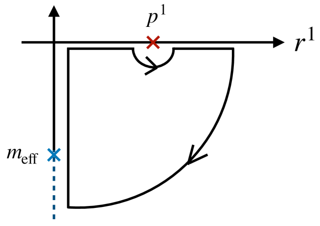
Figure 1: The contour used to evaluate (47) with clockwise orientation, avoiding the pole at $r^{1}=p^{1}$. The dotted blue line shows the brunch cut.

$$2\int_{0}^{\infty}\frac{dr^{1}}{2\pi 2E_{\vec{r}}}\frac{e^{\mathrm{i}t(E_{\vec{p}}-E_{\vec{r}})}}{E_{\vec{r}}-E_{\vec{p}}}=-\frac{\mathrm{i}}{2|p^{1}|}-\frac{\mathrm{i}}{\pi}\int_{0}^{m_{\mathrm{eff}}}\frac{d\rho}{\sqrt{m_{\mathrm{eff}}^{2}-\rho^{2}}}\frac{e^{\mathrm{i}t(E_{\vec{p}^{\prime}}-\sqrt{m_{\mathrm{eff}}^{2}-\rho^{2}})}}{\sqrt{m_{\mathrm{eff}}^{2}-\rho^{2}}-E_{\vec{p}}}+\mathcal{O}(e^{-mt}).$$ (47)

Similarly $A_{2}(l^{\prime};l)$ can be calculated as

$$2p^{1}\int_{0}^{\infty}\frac{dr^{1}}{2\pi 2E_{\vec{r}}}\frac{e^{\mathrm{i}t(E_{\vec{p}}-E_{\vec{r}})}}{(E_{\vec{r}}-E_{\vec{p}})(E_{\vec{r}}-E_{\vec{q}})} =\frac{\mathrm{i}q^{1}}{2(E_{\vec{p}}-E_{\vec{q}})}\Bigl{(}\frac{1}{|q^{1}|}e^{\mathrm{i}t(E_{\vec{p}}-E_{\vec{q}})}-\frac{1}{|p^{1}|}\Bigr{)}$$

$$\quad-\frac{\mathrm{i}p^{1}}{\pi}\int_{0}^{m_{\mathrm{eff}}}\frac{d\rho}{\sqrt{m_{\mathrm{eff}}^{2}-\rho^{2}}}\frac{e^{\mathrm{i}t(\sqrt{m_{\mathrm{eff}}^{2}-\rho^{2}}-E_{\vec{q}})}}{(\sqrt{m_{\mathrm{eff}}^{2}-\rho^{2}}-E_{\vec{p}})(\sqrt{m_{\mathrm{eff}}^{2}-\rho^{2}}-E_{\vec{q}})}$$

$$\quad+\mathcal{O}(e^{-mt}).$$ (48)

With the help of the relation (43), combining everything together yields

$$A_{1}(l^{\prime};l)+A_{2}(l^{\prime};l)=\mathrm{oscillatory\ terms}+\begin{cases}-\pi\bar{u}^{s^{\prime}}(p)\gamma^{1}u^{s}(q)\delta_{t}(E_{\vec{p}}-E_{\vec{q}})\delta_{c,1}&\text{$p^{1},q^{1}>0$}\\ -\pi\bar{u}^{s^{\prime}}(p)\gamma^{1}u^{s}(q)\delta^{\prime}_{t}(E_{\vec{p}}-E_{\vec{q}})\delta_{c,1}&\text{$p^{1}<0<q^{1}$}\\ \pi\bar{u}^{s^{\prime}}(p)\gamma^{1}u^{s}(q)\delta^{\prime}_{t}(E_{\vec{p}}-E_{\vec{q}})\delta_{c,1}&\text{$q^{1}<0<p^{1}$}\\ \pi\bar{u}^{s^{\prime}}(p)\gamma^{1}u^{s}(q)\delta_{t}(E_{\vec{p}}-E_{\vec{q}})\delta_{c,1}&\text{$p^{1},q^{1}<0$}\end{cases},$$ (49)

with $\delta^{\prime}_{t}(p)=(e^{\mathrm{i}tp}+1)/2\pi\mathrm{i}p$. The oscillatory terms in fact vanish as $t$ becomes large: see Appendix B. In the same manner we also find $\tilde{A}_{1}(l^{\prime};l)+\tilde{A}_{2}(l^{\prime};l)=-A_{1}(l^{\prime};l)-A_{2}(l^{\prime};l)$, implying $A_{1}(l^{\prime};l)+A_{2}(l^{\prime};l)+\tilde{A}_{1}(l^{\prime};l)+\tilde{A}_{2}(l^{\prime};l)=0$. The same story holds for $B$’s as well, namely

$$B_{1}(l^{\prime};l)+B_{2}(l^{\prime};l)=\mathrm{oscillatory\ terms}+\begin{cases}\pi\bar{v}^{s^{\prime}}(q)\gamma^{1}v^{s}(p)\delta_{t}(E_{\vec{p}}-E_{\vec{q}})\delta_{c,1}&\text{$p^{1},q^{1}>0$}\\ \pi\bar{v}^{s^{\prime}}(q)\gamma^{1}v^{s}(p)\delta^{\prime}_{t}(E_{\vec{p}}-E_{\vec{q}})\delta_{c,1}&\text{$p^{1}<0<q^{1}$}\\ -\pi\bar{v}^{s^{\prime}}(q)\gamma^{1}v^{s}(p)\delta^{\prime}_{t}(E_{\vec{p}}-E_{\vec{q}})\delta_{c,1}&\text{$q^{1}<0<p^{1}$}\\ -\pi\bar{v}^{s^{\prime}}(q)\gamma^{1}v^{s}(p)\delta_{t}(E_{\vec{p}}-E_{\vec{q}})\delta_{c,1}&\text{$p^{1},q^{1}<0$}\end{cases},$$ (50)

and $B_{1}(l^{\prime};l)+B_{2}(l^{\prime};l)+\tilde{B}_{1}(l^{\prime};l)+\tilde{B}_{2}(l^{\prime};l)=0$. Hence merging everything together, upon taking the large $t$ limit, we obtain

$$\langle\vec{p},c^{\prime},s^{\prime}|\sigma^{\prime}(t)|\vec{q},c,s\rangle=0,$$ (51)

and automatically $\langle\vec{p},c^{\prime},s^{\prime}|\sigma^{\prime\prime}(t)|\vec{q},c,s\rangle=0$. Moreover utilizing the building blocks we computed above, we find

$$\langle\vec{p},c^{\prime},s^{\prime}|\sigma(t)^{2}|\vec{q},c,s\rangle =\begin{cases}\bar{u}^{s^{\prime}}(p)\gamma^{1}u^{s}(q)W_{\vec{p},\vec{q}}&\text{$c=+1$}\\ \bar{v}^{s^{\prime}}(q)\gamma^{1}v^{s}(p)W_{\vec{p},\vec{q}}&\text{$c=-1$}\end{cases},$$ (52)

where

$$W_{\vec{p},\vec{q}}=\begin{cases}\hat{\delta}_{t}^{(3)}(\vec{p}-\vec{q})&\text{$p^{1},q^{1}>0$}\\ \hat{\delta}_{t}^{\prime(3)}(\vec{p}-\vec{q})&\text{$p^{1}<0<q^{1}$}\\ -\hat{\delta}_{t}^{\prime(3)}(\vec{p}-\vec{q})&\text{$q^{1}<0<p^{1}$}\\ -\hat{\delta}_{t}^{(3)}(\vec{p}-\vec{q})&\text{$p^{1},q^{1}<0$}\end{cases},$$ (53)

with $\hat{\delta}_{t}^{\prime(3)}(\vec{p}-\vec{q})=(2\pi)^{3}\delta^{(2)}(\tilde{p}^{\prime}-\tilde{q})\delta^{\prime}_{t}(E_{\vec{p}}-E_{\vec{q}})$. We now put everything into (34) and obtain, for fermions ($c=1$)

$$\langle\vec{p},c^{\prime},s^{\prime}|e^{\theta_{\lambda,\gamma}(t)}-1|\vec{q},c,s\rangle =\begin{cases}(e^{\mathrm{i}\lambda}-1)\bar{u}^{s^{\prime}}(p)\gamma^{1}u^{s}(q)\hat{\delta}_{t}^{(3)}(\vec{p}-\vec{q})\delta_{c^{\prime},c}&\text{$p^{1},q^{1}>0$}\\ (e^{\mathrm{i}\lambda}-1)\bar{u}^{s^{\prime}}(p)\gamma^{1}u^{s}(q)\hat{\delta}_{t}^{\prime(3)}(\vec{p}-\vec{q})\delta_{c^{\prime},c}&\text{$p^{1}<0<q^{1}$}\\ (1-e^{-\mathrm{i}\lambda})\bar{u}^{s^{\prime}}(p)\gamma^{1}u^{s}(q)\hat{\delta}_{t}^{\prime(3)}(\vec{p}-\vec{q})\delta_{c^{\prime},c}&\text{$q^{1}<0<p^{1}$}\\ (1-e^{-\mathrm{i}\lambda})\bar{u}^{s^{\prime}}(p)\gamma^{1}u^{s}(q)\hat{\delta}_{t}^{(3)}(\vec{p}-\vec{q})\delta_{c^{\prime},c}&\text{$p^{1},q^{1}<0$},\end{cases}$$ (54)

and for antifermions ($c=-1$)

$$\langle\vec{p},c^{\prime},s^{\prime}|e^{\theta_{\lambda,\gamma}(t)}-1|\vec{q},c,s\rangle =\begin{cases}(e^{-\mathrm{i}\lambda}-1)\bar{v}^{s^{\prime}}(q)\gamma^{1}v^{s}(p)\hat{\delta}_{t}^{(3)}(\vec{p}-\vec{q})\delta_{c^{\prime},c}&\text{$p^{1},q^{1}>0$}\\ (e^{-\mathrm{i}\lambda}-1)\bar{v}^{s^{\prime}}(q)\gamma^{1}v^{s}(p)\hat{\delta}_{t}^{\prime(3)}(\vec{p}-\vec{q})\delta_{c^{\prime},c}&\text{$p^{1}<0<q^{1}$}\\ (1-e^{\mathrm{i}\lambda})\bar{v}^{s^{\prime}}(q)\gamma^{1}v^{s}(p)\hat{\delta}_{t}^{\prime(3)}(\vec{p}-\vec{q})\delta_{c^{\prime},c}&\text{$q^{1}<0<p^{1}$}\\ (1-e^{\mathrm{i}\lambda})\bar{v}^{s^{\prime}}(q)\gamma^{1}v^{s}(p)\hat{\delta}_{t}^{(3)}(\vec{p}-\vec{q})\delta_{c^{\prime},c}&\text{$p^{1},q^{1}<0$}.\end{cases}$$ (55)

3.3 Levitov-Lesovik formula in 3+1 dimensions

The quantity we are initially interested in is the long-time limit of the cumulant generating function (29). By means of Klich’s trace formula [13], it was shown in [18] that the generating function can be expressed in the following form:

$$\mathrm{Tr}(\rho_{\mathrm{s}}e^{\Theta_{\lambda,\gamma}(t)})=\det\bigl{(}1+n_{\mathrm{s}}(e^{\theta_{\lambda,\gamma}(t)}-1)\bigr{)},$$ (56)

where

$$\langle\vec{p},c^{\prime},s^{\prime}|n_{\mathrm{s}}|\vec{q},c,s\rangle=\begin{cases}n_{+}(\vec{p})2E_{\vec{p}}(2\pi)^{3}\delta^{(3)}(\vec{p}-\vec{q})\delta_{c^{\prime}c}\delta_{s,s^{\prime}}&\text{$c=1$}\\ n_{-}(\vec{p})2E_{\vec{p}}(2\pi)^{3}\delta^{(3)}(\vec{p}-\vec{q})\delta_{c^{\prime}c}\delta_{s,s^{\prime}}&\text{$c=-1$}\end{cases}$$ (57)

with $n_{\pm}(\vec{p})=1/(e^{V_{\pm}(\vec{p})}-1)$. Note that the trace on the LHS is done over the full Hilbert space, while the determinant on the RHS is over the one-particle Hilbert space.
 It can be readily shown that for $t\to\infty$, contributions from the diagonal matrix elements become dominant, and we find

$$\log\mathrm{Tr}(\rho_{\mathrm{s}}e^{\Theta_{\lambda,\gamma}(t)}) =2tL^{2}\sum_{\epsilon=\pm}\int\frac{d^{2}{\tilde{p}}}{(2\pi)^{2}}$$

$$\quad\times\int_{m_{\mathrm{eff}}(\tilde{p})}^{\infty}\frac{dE}{2\pi}\log\bigl{[}1+n_{\epsilon,\mathrm{L}}(n_{\epsilon,\mathrm{R}}-1)(1-e^{\mathrm{i}\epsilon\lambda})+n_{\epsilon,\mathrm{R}}(n_{\epsilon,\mathrm{L}}-1)(1-e^{-\mathrm{i}\epsilon\lambda})\bigr{]},$$ (58)

where $n_{\epsilon;\mathrm{L},\mathrm{R}}(E)$ are fermionic filling functions defined as

$$n_{\epsilon;\mathrm{L},\mathrm{R}}(E)=\frac{1}{e^{\beta_{\mathrm{L},\mathrm{R}}(E-\epsilon\mu_{\mathrm{L},\mathrm{R}})}+1}.$$ (59)

Hence the desired scaled cumulant generating function is

$$F(\lambda) =2\sum_{\epsilon=\pm}\int\frac{d^{2}{\tilde{p}}}{(2\pi)^{2}}\int_{m_{\mathrm{eff}}(\tilde{p})}^{\infty}\frac{dE}{2\pi}\log\bigl{[}1+n_{\epsilon,\mathrm{L}}(n_{\epsilon,\mathrm{R}}-1)(1-e^{\mathrm{i}\epsilon\lambda})+n_{\epsilon,\mathrm{R}}(n_{\epsilon,\mathrm{L}}-1)(1-e^{-\mathrm{i}\epsilon\lambda})\bigr{]}.$$

$$:=f(\lambda;\beta_{\mathrm{L}},\beta_{\mathrm{L}}\mu_{\mathrm{L}})+f(-\lambda;\beta_{\mathrm{R}},\beta_{\mathrm{R}}\mu_{\mathrm{R}}),$$ (60)

where $f(\lambda;\beta,\beta\mu)$ is given by

$$f(\lambda;\beta,\beta\mu)=2\sum_{\epsilon=\pm}\int\frac{d^{2}{\tilde{p}}}{(2\pi)^{2}}\int_{m_{\mathrm{eff}}(\tilde{p})}^{\infty}\frac{dE}{2\pi}\log\bigl{[}1+n_{\epsilon}(e^{\mathrm{i}\epsilon\lambda}-1)\bigr{]}.$$ (61)

Some comments are in order. We first notice that this can be seen as a simple relativistic generalization of the celebrated Levitov-Lesovik formula [20] in three spatial dimensions. The two possible spins and charges are responsible for a prefactor 2 and a sum over two signs $\epsilon=\pm$ respectively. Note that all transmission coefficients are 1 as this is a free model without impurities. Thanks to this fact the SCGF factorizes as (60), and consequently enables us to have a clear interpretation of it: the SCGF associated with the charge transport is a sum of independent Bernoulli processes. Recall that the Bernoulli process is a time-discrete stochastic process whose possible events at each frame (trial of a jump) are only either success or failure of the jump. For instance a fermion that was initially prepared in the left (resp. right) subsystem with energy $E$ and charge 1 (the value of spin does not matter) is transferred from left to right (resp. from right to left) with a success probability $n_{+,\mathrm{L}}(E)$ (resp. $n_{+,\mathrm{R}}(E)$), thus has a SCGF $\log[1+n_{+,\mathrm{L}}(E)(e^{\mathrm{i}\lambda}-1)]$ (resp. $\log[1+n_{+,\mathrm{R}}(E)(e^{-\mathrm{i}\lambda}-1)]$). The number of fermions that jump successfully during time $t$ has then a Binomial distribution $B(n_{t},p)$ where $n_{t}$ is the number of trials during time $t$, and the probability of obtaining $k$ successes $P(k;n_{t},p)$ is given by

$$P(k;n_{t},p)=\begin{pmatrix}n_{t}\\ p\end{pmatrix}p^{k}(1-p)^{n_{t}-k}.$$ (62)

Since the CGF of independent processes are additive, we can obtain the SCGF (60) by integrating and summing over energy and charge. This interpretation for the charge transport in the Dirac theory would hold in any dimension. It is illuminating to contrast this Bernoullian interpretation for the charge transport with the Poissonian interpretation for the energy transport in higher dimensional free models and 2D conformal field theories [1, 3, 7], which indicates that energy quanta and charge quanta are transferred according to different statistics in those systems.   We also observe that when the two temperatures are equal $T_{\mathrm{L}}=T_{\mathrm{R}}=T$, this formula satisfies the fluctuation theorem: $F(\lambda)=F(-\lambda+\mathrm{i}(\mu_{\mathrm{L}}-\mu_{\mathrm{R}})/T)$ [27]. This is also evident as a consequence of the time-reversal symmetry of the Dirac theory [24]. Performing the integral, we can derive the analytic expression (see Appendix D) of the chiral SCGF (61) which reads

$$f(\lambda;\beta,\beta\mu)= -\sum_{\epsilon=\pm}\sum_{n=1}^{\infty}\frac{(-1)^{n}(1+\beta mn)}{2\pi^{2}\beta^{3}n^{4}}e^{-\beta n(m-\epsilon\mu)}(e^{\mathrm{i}\epsilon\lambda n}-1) |\mu|<m$$ (63a)

$$f(\lambda;\beta,\beta\mu)= f_{0}(\lambda;\beta,\mu)+f_{\mathrm{M}}(\lambda;\beta,\mu) m<\mu$$ (63b)

$$f(\lambda;\beta,\beta\mu)= f_{0}(\lambda;\beta,\mu)+f_{\mathrm{M}}(-\lambda;\beta,-\mu) m<-\mu$$ , (63c)

where we defined $f_{0}(\lambda,\beta,\mu)$, which is the massless limit of (61), and $f_{\mathrm{M}}(\lambda;\beta,\mu)$ as

$$f_{0}(\lambda;\beta,\beta\mu) =\frac{\mathrm{i}\mu^{3}\lambda}{12\pi^{2}}-\frac{1}{2\pi^{2}\beta^{3}}\sum_{\epsilon=\pm}\sum_{n=1}^{\infty}\frac{(-1)^{n}}{n^{4}}\frac{1+(1+\epsilon\mu\beta n)^{2}}{2}(e^{\mathrm{i}\epsilon\lambda n}-1)$$ (64)

$$f_{\mathrm{{M}}}(\lambda;\beta,\beta\mu) =\frac{\mathrm{i}m^{2}}{12\pi^{2}}(2m-3\mu)\lambda+\frac{1}{\pi^{2}\beta^{3}}\sum_{n=1}^{\infty}\frac{(-1)^{n}}{n^{4}}\biggl{[}\frac{\beta^{2}m^{2}n^{2}}{4}(e^{\mathrm{i}\lambda n}-1)$$

$$\ +\Bigl{\{}e^{-\beta\mu n}(\sinh(\beta mn)-\beta mn\cosh(\beta mn))+\frac{\beta^{2}m^{2}n^{2}}{4}\Bigr{\}}(e^{-\mathrm{i}\lambda n}-1)\biggr{]}.$$ (65)

That the SCGFs at $m<\mu$ and $m<-\mu$ have similar forms is due to the charge conjugation symmetry in the Dirac theory. It is worth noting that the parity symmetry, a symmetry under the swapping of left- and right-handed spinors, plays no role here since the distinction between the two spinors does not affect anything in the charge transport. Those SCGFs basically comprise (possibly) a linear term and a sum of Poisson-like terms with coefficients that are not necessarily positive. The linear term in fact represents a perfect transmission [28]: perfect transmission means a transfer with the success probability 1 now, hence the corresponding SCGF is $\log(1+e^{\mathrm{i}\lambda}-1)=\mathrm{i}\lambda$ (modulo $2\pi$).

There is one more thing that deserves to be detailed. For ease of explanation we shall assume $\mu>0$ hereafter. Let us remind that as a consequence of the charge quantization, our SCGF has a periodicity $F(\lambda)=F(\lambda+2\pi)$ as do other CGFs associated with charge transfers. It is then natural to ask how the SCGF looks like in the fundamental domain $(-\pi,\pi)$. Further restricting our attention to the case $m<\mu$, when $\lambda\in(-\pi,\pi)$, the series in (64) and (65) converge, yielding

$$f_{0}(\lambda;\beta,\beta\mu) =\frac{1}{12\pi^{2}\beta^{3}}\Bigl{[}\frac{1}{4}(\beta\mu+\mathrm{i}\lambda)^{4}-\frac{1}{4}(\beta\mu)^{4}+\frac{\pi^{2}}{2}(\beta\mu+\mathrm{i}\lambda)^{2}-\frac{\pi^{2}}{2}(\beta\mu)^{2}\Bigr{]},$$ (66)

$$f_{\mathrm{M}}(\lambda;\beta,\beta\mu) =\frac{\mathrm{i}m^{3}\lambda}{6\pi^{2}}-\frac{m^{2}}{8\pi^{2}\beta}\bigl{[}(\beta\mu+\mathrm{i}\lambda)^{2}-(\beta\mu)^{2}\bigr{]}$$

$$\quad-\frac{1}{\pi^{2}\beta^{3}}\sum_{n=1}^{\infty}\frac{(-1)^{n}}{n^{4}}e^{-\beta\mu n}(\sinh(\beta mn)-\beta mn\cosh(\beta mn))(e^{-\mathrm{i}\lambda n}-1).$$ (67)

In the massless case, the SCGF becomes a finite polynomial of $\lambda$ by virtue of the presence of both fermions and antifermions in this model. Therefore we have cumulants only up to fourth order. Notice, however, that this does not mean that the full SCGF is also a finite polynomial - it is not analytic (not Taylor expandable) in the entire domain. In fact when $m<\mu$, it is not even differentiable, which amounts to a quantitatively different behavior of the charge current depending on $m\gtrless\mu$ as we shall see below.

Before focusing on the charge current, let us introduce the notion of large deviation function (LDF) $I(J)$ defined as the Legendre transform of the SCGF (60)

$$I(J)=\max_{\lambda\in\mathbb{R}}(\lambda J-F(\lambda)).$$ (68)

This function inherits the convexity of $F(\lambda)$ and takes its minimum, which is zero, when $J=\langle J_{Q}\rangle$ where $\langle J_{Q}\rangle$ is the NESS charge current. Thus the function $-I(J)$ bears a similarity with entropy in equilibrium that is maximized by the (generalized) thermal state. As seen in Fig.2, the chiral LDF $\iota(j)\equiv\max_{\lambda\in\mathbb{R}}(\lambda j-f(\lambda))$, hence the full LDF, indeed satisfies the above properties of generic LDFs.

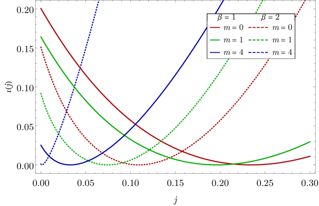
Figure 2: The chiral LDF (CLDF) $\iota(j)$ is depicted with $\mu=2$ varying the mass $m$ and the inverse temperature $\beta$. The value of the mass is chosen so that the lines with different colors correspond to different regimes (red, green and blue lines are for massless $m=0$, small-mass $m<\mu$, and large-mass $m>\mu$ regimes respectively). Solid lines correspond to the CLDF for $\beta=1$ while dashed lines describes that for $\beta=2$. As explained in the main text, $j$’s at which the CLDF takes its minimum is the value of the chiral NESS current $j=\langle j_{Q}\rangle$. We observe that as the temperature decreases, the chiral NESS current in the large-mass phase becomes distinctively small compared to those in other regimes.

Once we obtain the SCGF, its multiple differentiations with respect to $\lambda$ evaluated at $\lambda=0$ yield all the cumulants. In particular, the average of the charge current in the NESS $\langle J_{Q}(\beta_{\mathrm{L}},\beta_{\mathrm{L}}\mu_{\mathrm{L}};\beta_{\mathrm{R}},\beta_{\mathrm{R}}\mu_{\mathrm{R}})\rangle=\left.dF(\lambda)/d(\mathrm{i}\lambda)\right|_{\lambda=0}$ is of great importance in actual experiments. The chiral part $\langle j_{Q}(\beta,\beta\mu)\rangle=\left.df(\lambda;\beta,\beta\mu)/d(\mathrm{i}\lambda)\right|_{\lambda=0}$ reads,

$$\langle j_{Q}(\beta,\beta\mu)\rangle=\begin{dcases*}\mathcal{O}(\beta^{-2})&$\mu<m$\\ \frac{\mu^{3}}{12\pi^{2}}+\frac{m^{3}}{6\pi^{2}}-\frac{m^{2}\mu}{8\pi^{2}}+\frac{\mu}{12\beta^{2}}+\frac{m}{12\beta^{2}}+\mathcal{O}(\beta^{-2})&$m<\mu$.\end{dcases*}$$ (69)

The phase $\mu<m$ can be considered as an insulating phase in the sense that the charge current is effectively zero in the low temperature limit: jumps made by particles are less probable because the occupation function $n(E)$, which is supposed to be the probability of each jump, can take a value only less than one half (see Fig.2). The existence of such phase is a peculiarity in Dirac theory which is forbidden in non-relativistic free fermionic systems (see Appendix F). It is also of particular interest to observe its massless limit since most Dirac fermions that exist as low-energy theories in unconventional matters such as Dirac semimetals are massless. The current in the massless limit is given exactly by

$$\langle J_{Q}(\beta_{\mathrm{L}},\beta_{\mathrm{L}}\mu_{\mathrm{L}};\beta_{\mathrm{R}},\beta_{\mathrm{R}}\mu_{\mathrm{R}})\rangle=\frac{\mu^{3}_{\mathrm{L}}-\mu^{3}_{\mathrm{R}}+\pi^{2}(\mu_{\mathrm{L}}T^{2}_{\mathrm{L}}-\mu_{\mathrm{R}}T^{2}_{\mathrm{R}})}{12\pi^{2}}.$$ (70)

In the zero temperature limit, this reduces to $\langle J_{Q}(T_{\mathrm{L},\mathrm{R}}=0)\rangle=(\mu_{\mathrm{L}}^{3}-\mu_{\mathrm{R}}^{3})/12\pi^{2}$, which can be expected given the chiral separation (60) and on the basis of dimensional analysis. We expect that this is generalized to $\langle J_{Q}(T_{\mathrm{L},\mathrm{R}}=0)\rangle\propto\mu_{\mathrm{L}}^{d}-\mu_{\mathrm{R}}^{d}$ in $d$ spatial dimensional Dirac models.

3.4 Extended fluctuation relation

It was advocated in [24] that if systems whose dynamics satisfy the pure tansmission condition $S\tilde{Q}=-\tilde{Q}S$, the extended fluctuation relation (EFR) holds. Here $S=S_{-}^{-1}S_{+}$ with $S_{-}=\lim_{t\to-\infty}e^{-\mathrm{i}tH}e^{\mathrm{i}tH_{0}}$ is the $S$-matrix, and for the charge transport the EFR reads

$$F(\lambda)=\int_{0}^{\mathrm{i}\lambda}dz\langle J_{Q}(\beta_{\mathrm{L}},\beta_{\mathrm{L}}\mu_{\mathrm{L}}+z;\beta_{\mathrm{R}},\beta_{\mathrm{R}}\mu_{\mathrm{R}}-z)\rangle$$ (71)

or alternatively, due to the factorization (60),

$$f(\lambda;\beta,\beta\mu)=\int_{0}^{\mathrm{i}\lambda}dz\langle j_{Q}(\beta,\beta\mu+z)\rangle.$$ (72)

It is immediate to see that the Dirac theory indeed satisfies it: let us again focus on the massless case where $\langle j_{Q}(\beta,\beta\mu)\rangle=(\beta^{3}\mu^{3}+\pi^{2}\beta\mu)/12\pi^{2}\beta^{3}$. Upon shifting $\beta\mu\mapsto\beta\mu+z$ and an integral over $z$, (66) is reproduced. Once we obtain (66), a representation of the SCGF for the entire domain, (64), is computed as a Fourier series. Thus we need only the average of the current to acquire the SCGF (all other higher cumulants are unnecessary). Notice that in the course of deriving Fourier coefficients, we need to figure out terms associated with perfect transmission. In order to see this, we can take a zero temperature limit $\beta\to\infty$ where thermal fluctuation is negligible: remaining terms, in our case $\mathrm{i}\mu^{3}\lambda/12\pi^{2}$, are the sought ones.

Finally let us emphasize why EFR is useful. The approach we have taken, which is based on the two-point von Neumann measurement, enables us to directly compute the SCGF. In view of that approach, one might find that the EFR is just a curious relation. However, when one knows the average current first rather than having the SCGF first (for instance, this is the case in hydrodynamics), EFR becomes extremely powerful: one can obtain the SCGF just by integrating the current with shifting parameters properly. We demonstrate how we can gain the SCGF for the energy transport in Appendix E as well as reporting the SCGF that combines both charge and energy transports. Furthermore, for a comparison, we briefly examine the charge transport in the Lifshitz fermions (i.e. non-relativistic fermion system with a dispersion relation $E=|p|^{z}/2m$) in Appendix F.

4 Discussion and conclusion

In this manuscript we have studied the non-equilibrium $U(1)$ charge transport of the Dirac theory. We derived the NESS density operator in the same spirit as [7], and computed the SCGF associated with the charge transport. The so-determined SCGF was then interpreted as an extension of the Levitov-Lesovik formula to higher dimensions. Remarkably, in the massless limit, cumulants of the SCGF exist up to fourth order. We expect that, generically, in $D$ space-time dimensions, the cumulants are nonzero only up to $D$-th order. We also found an insulating regime, which does not exist in the non-relativistic free fermion systems, where the NESS current is negligibly small for small temperatures. Finally the validity of the EFR for the charge transfer was confirmed. One of natural extensions of our results would be to consider an impurity at the junction $x^{1}=0$ [29, 30], giving rise to the transmission coefficient $T(p^{1})$ that is not unity. In this case, we still expect that the chiral SCGF takes a similar form as (61):

$$f(\lambda;\beta,\beta\mu)=2\sum_{\epsilon=\pm}\int\frac{d^{2}{\tilde{p}}}{(2\pi)^{2}}\int_{m_{\mathrm{eff}}(\tilde{p})}^{\infty}\frac{dE}{2\pi}\log\bigl{[}1+Tn_{\epsilon}(e^{\mathrm{i}\epsilon\lambda}-1)\bigr{]}.$$ (73)

This would be straightforwardly derived by writing down the NESS density operator with taking accounting of the impurity [31].

Another possible generalization could be extending to generic spacial dimensions $d$. To do so, one should be aware of the different nature of the spinor representation of $SO(d,1)$ in even and odd dimensions: in odd spatial dimensions there exist Weyl spinors, but this is not the case in even spatial dimensions. It would be of course interesting to study the effect of interactions, but for that purpose, our approach might not be the most efficient way. Instead, focusing on the long-wavelength physics, one can study the dynamics of the Dirac fermions as the Dirac fluid [32, 33].

5 Acknowledgements

I thank Benjamin Doyon and Joe Bhaseen for useful discussions, and acknowledge the support of the Takenaka scholarship foundation. This work is also partly supported by the ERC advanced grant NuQFT.

Appendix A Time-evolution in B-representation

In this section, we explicitly demonstrate that $\psi_{\rm B}(\vec{x},t)=\lim_{t\to\infty}S(\psi_{\rm A}(\vec{x},t))$ [7]. By construction, it is immediate to see that

$$\psi_{{\rm B},a}(\vec{x},t)=\sum_{b}\int d^{3}y\{\psi_{{\rm A},a}(\vec{x},t),\psi^{\dagger}_{{\rm A},b}(\vec{y})\}\psi_{{\rm B},b}(\vec{y})$$ (74)

solves the equation motion of the Dirac theory $(i\gamma^{\mu}\partial_{\mu}-m)\psi_{{\rm B},a}(\vec{x},t)=0$. The anticommutator $\{\psi_{{\rm A},a}(\vec{x},t),\psi^{\dagger}_{{\rm A},b}(\vec{y})\}$ is readily evaluated by the direct computation:

$$\{\psi_{{\rm A},a}(\vec{x},t),\psi^{\dagger}_{{\rm A},b}(\vec{y})\} =\int\frac{d^{3}p}{(2\pi)^{3}2E_{\vec{p}}}\sum_{s}\bigl{[}u^{s}_{a}(p)u^{s\dagger}_{b}(p)e^{-\mathrm{i}E_{\vec{p}}t}+v^{s}_{a}(\bar{p})v^{s\dagger}_{b}(\bar{p})e^{\mathrm{i}E_{\vec{p}}t}\bigr{]}e^{\mathrm{i}\vec{p}\cdot(\vec{x}-\vec{y})}$$

$$=\int\frac{d^{3}p}{(2\pi)^{3}2E_{\vec{p}}}\sum_{s}\mathbb{M}_{ab}^{s}(\vec{p},t)e^{\mathrm{i}\vec{p}\cdot(\vec{x}-\vec{y})},$$ (75)

where $\bar{p}=(p^{0},-\vec{p})$ and $\mathbb{M}_{ab}^{s}(\vec{p},t):=u^{s}_{a}(p)u^{s\dagger}_{b}(p)e^{-\mathrm{i}E_{\vec{p}}t}+v^{s}_{a}(\bar{p})v^{s\dagger}_{b}(\bar{p})e^{\mathrm{i}E_{\vec{p}}t}$. Plugging this and (17) into (74), we have

$$\psi_{{\rm B},a}(\vec{x},t) =\sum_{s,s^{\prime},b}\int Dqe^{\mathrm{i}\tilde{q}\cdot\tilde{x}}\int_{0}^{\infty}\frac{dp^{1}}{2\pi}\frac{\mathrm{sgn}(q^{1})}{2E_{p^{1},\tilde{q}}}\bigl{[}\mathbb{M}_{ab}^{s}(p^{1},\tilde{q},t)\mathbb{U}_{1}(p^{1},q^{1})A^{s^{\prime}}_{q}u^{s^{\prime}}(q)e^{\mathrm{i}p^{1}x^{1}}+\{p^{1}\leftrightarrow-p^{1}\}\bigr{]}$$

$$\quad+\sum_{s,s^{\prime},b}\int Dqe^{-\mathrm{i}\tilde{q}\cdot\tilde{x}}\int_{0}^{\infty}\frac{dp^{1}}{2\pi}\frac{\mathrm{sgn}(q^{1})}{2E_{p^{1},-\tilde{q}}}\bigl{[}\mathbb{M}_{ab}^{s}(p^{1},-\tilde{q},t)\mathbb{U}_{2}(p^{1},q^{1})B^{\dagger s^{\prime}}_{q}v^{\dagger s^{\prime}}(q)e^{\mathrm{i}p^{1}x^{1}}+\{p^{1}\leftrightarrow-p^{1}\}\bigr{]},$$ (76)

where $E_{p^{1},\tilde{q}}=\sqrt{(p^{1})^{2}+|\tilde{q}|^{2}+m^{2}}$, and $\mathbb{U}_{1}(p^{1},q^{1})$ and $\mathbb{U}_{2}(p^{1},q^{1})$ are given by

$$\mathbb{U}_{1}(p^{1},q^{1})=\frac{\mathrm{i}}{p^{1}-q^{1}-\mathrm{i}0}+\frac{\mathrm{i}}{p^{1}-q^{1}+\mathrm{i}0},\quad\mathbb{U}_{2}(p^{1},q^{1})=\frac{\mathrm{i}}{p^{1}+q^{1}-\mathrm{i}0}+\frac{\mathrm{i}}{p^{1}+q^{1}+\mathrm{i}0}.$$ (77)

In order to evaluate these integrals, we need to deform the contours of $p^{1}$-integral to either $(0,\mathrm{i}\infty)$ or $(0,-\mathrm{i}\infty)$. To which direction we deform the contours is determined in such a way that there is no contribution at infinity, and depends on the sign of $p^{1}$ and $x^{1}$ in exponentials (see Appendix C in [7] for more detailed expositions). For instance, when we compute the first term of the first line in (A) we have $e^{-\mathrm{i}E_{\vec{p}}t+\mathrm{i}p^{1}x^{1}}$ and $e^{\mathrm{i}E_{\vec{p}}t+\mathrm{i}p^{1}x^{1}}$ for which we deform the contour of the $p^{1}$-integral to $(0,\mathrm{i}\infty)$ and $(0,-\mathrm{i}\infty)$, respectively. Hence we need to evaluate only a single pole at $p^{1}=q^{1}$ which gives rise to the terms that contain $\sum_{b}u^{s}_{a}(q^{1},\tilde{q})u^{s\dagger}_{b}(q^{1},\tilde{q})u^{s^{\prime}}_{b}(q^{1},\tilde{q})=2E_{\vec{q}}u^{s}_{a}(q^{1},\tilde{q})\delta^{ss^{\prime}}$ and $\sum_{b}v^{s}_{a}(-q^{1},-\tilde{q})v^{s\dagger}_{b}(-q^{1},-\tilde{q})u^{s^{\prime}}_{b}(q^{1},\tilde{q})=0$, thanks to the fact that $u$’s and $v$’s are orthogonal: $\sum_{b}v^{s\dagger}_{b}(-\vec{p})u^{s^{\prime}}_{b}(\vec{p})=0$. Likewise, we can extract contributions from poles $p^{1}=\pm q^{1}$ in other terms, and we end up with the following

$$\psi_{{\rm B},a}(\vec{x},t)=\int Dp\sum_{s}(A_{\vec{p}}^{s}u^{s}_{a}(p)e^{-\mathrm{i}p\cdot x}+B_{\vec{p}}^{s\dagger}v^{s}_{a}(p)e^{\mathrm{i}p\cdot x})+{\rm integral\ contribution}.$$ (78)

In the exactly same manner as in [7], we can show that this integral contribution provides no contribution when we take the average of any observable $\mathcal{O}$ that involves $\psi(\vec{x},t),\psi^{\dagger}(\vec{x},t)$, and their derivatives, at $t\to\infty$.

Appendix B Large-$t$ behavior of oscillatory terms

One can explicitly show that the oscillatory that appeared in computing matrix elements terms do not contribute to results, i.e. decay under $t\to\infty$. Following [7], We exemplify it by calculating one of them which appeared in (47):

$$\int_{0}^{m_{\mathrm{eff}}}\frac{d\rho}{\sqrt{m_{\mathrm{eff}}^{2}-\rho^{2}}}\frac{e^{\mathrm{i}t(E_{\vec{p}^{\prime}}-\sqrt{m_{\mathrm{eff}}^{2}-\rho^{2}})}}{\sqrt{m_{\mathrm{eff}}^{2}-\rho^{2}}-E_{\vec{p}^{\prime}}}=\int_{0}^{m_{\mathrm{eff}}}\frac{dr}{\sqrt{m_{\mathrm{eff}}^{2}-r^{2}}}\frac{e^{\mathrm{i}t(r-E_{\vec{p}^{\prime}})}}{r-E_{\vec{p}^{\prime}}}.$$ (79)

Other terms might be treated in a same fashion. We shall use contour deformations again to make the asymptotic analysis feasible. First we start with a rectangular on which the integral is performed in a complex plane parametrized by $z$. Vertical lines of the rectangular are located at, say $r=m_{\mathrm{eff}}+\mathrm{i}\mathrm{Im}(z)$ and $\mathrm{i}\mathrm{Im}(z)$ with $0\leq\mathrm{Im}(z)\leq v$, whereas horizontal lines are $[0,m_{\mathrm{eff}}]$ and $\mathrm{Re}(z)+\mathrm{i}v$ with $\mathrm{Re}(z)\in[0,m_{\mathrm{eff}}]$. Taking $v\to\infty$, the integral along the upper horizontal line vanishes. Thus changing variables properly, we have

$$\int_{0}^{m_{\mathrm{eff}}}\frac{dr}{\sqrt{m_{\mathrm{eff}}^{2}-r^{2}}}\frac{e^{\mathrm{i}tr}}{r-E_{\vec{p}^{\prime}}}=-\mathrm{i}\int_{0}^{\infty}\frac{due^{-ut}}{\sqrt{u^{2}-2\mathrm{i}m_{\mathrm{eff}}u}}\frac{e^{\mathrm{i}m_{\mathrm{eff}}t}}{m_{\mathrm{eff}}+\mathrm{i}u-E_{\vec{p}^{\prime}}}+\mathrm{i}\int_{0}^{\infty}\frac{du}{\sqrt{m_{\mathrm{eff}}^{2}+u^{2}}}\frac{e^{-ut}}{\mathrm{i}u-E_{\vec{p}^{\prime}}}.$$ (80)

For a large $t$, main contributions can be ontained by expanding integrands around $u=0$:

$$\int_{0}^{\infty}\frac{due^{-ut}}{\sqrt{u^{2}-2\mathrm{i}m_{\mathrm{eff}}u}}\frac{e^{\mathrm{i}m_{\mathrm{eff}}t}}{m_{\mathrm{eff}}+\mathrm{i}u-E_{\vec{p}^{\prime}}} \approx\frac{e^{\mathrm{i}m_{\mathrm{eff}}t}}{(m_{\mathrm{eff}}-E_{\vec{p}^{\prime}})\sqrt{2\mathrm{i}m_{\mathrm{eff}}}}\int_{0}^{\infty}du\frac{e^{-ut}}{u}\Bigl{(}1+\frac{u}{4\mathrm{i}m_{\mathrm{eff}}}\Bigr{)}\Bigl{(}1-\frac{\mathrm{i}u}{m_{\mathrm{eff}}-E_{\vec{p}^{\prime}}}\Bigr{)}$$

$$=\frac{e^{\mathrm{i}m_{\mathrm{eff}}t}}{(m_{\mathrm{eff}}-E_{\vec{p}^{\prime}})\sqrt{2\mathrm{i}m_{\mathrm{eff}}}}t^{-\frac{1}{2}}+\mathcal{O}(t^{-1}),$$ (81)

$$\int_{0}^{\infty}\frac{du}{\sqrt{m_{\mathrm{eff}}^{2}+u^{2}}}\frac{e^{-ut}}{\mathrm{i}u-E_{\vec{p}^{\prime}}} \approx-\frac{1}{m_{\mathrm{eff}}E_{\vec{p}^{\prime}}}\int_{0}^{\infty}due^{-ut}\Bigl{(}1-\frac{u^{2}}{2m_{\mathrm{eff}}^{2}}\Bigr{)}\Bigl{(}1+\frac{\mathrm{i}u}{E_{\vec{p}^{\prime}}}\Bigr{)}$$

$$=-\frac{1}{m_{\mathrm{eff}}E_{\vec{p}^{\prime}}}t^{-1}+\mathcal{O}(t^{-2}).$$ (82)

Combining everything together, under $t\to\infty$, we find that the oscillatory term decays algebraically with tails

$$\int_{0}^{m_{\mathrm{eff}}}\frac{d\rho}{\sqrt{m_{\mathrm{eff}}^{2}-\rho^{2}}}\frac{e^{\mathrm{i}t(E_{\vec{p}^{\prime}}-\sqrt{m_{\mathrm{eff}}^{2}-\rho^{2}})}}{\sqrt{m_{\mathrm{eff}}^{2}-\rho^{2}}-E_{\vec{p}^{\prime}}}=-\mathrm{i}\frac{e^{\mathrm{i}m_{\mathrm{eff}}t}}{(m_{\mathrm{eff}}-E_{\vec{p}^{\prime}})\sqrt{2\mathrm{i}m_{\mathrm{eff}}}}t^{-\frac{1}{2}}+\mathcal{O}(t^{-1}).$$ (83)

Appendix C Asymptotics

In this appendix we evaluate a logarithm of the determinant $\log\mathrm{det}_{\mathcal{H}_{1\mathrm{P}}}(1+AB(t))$ where one-particle operators $A$ and $B(t)$ have matrix elements

$$\langle\vec{p}|A|\vec{q}\rangle=A(\vec{p})2E_{\vec{p}}\,\hat{\delta}^{(3)}(\vec{p}-\vec{q}),\ \ \langle\vec{p}|B(t)|\vec{q}\rangle=B(\vec{p},\vec{q})2E_{\vec{p}}\,\hat{\delta}_{t}^{(3)}(\vec{p}-\vec{q}).$$ (84)

Remember that a logarithm of the determinant can be expressed as

$$\log\mathrm{det}_{\mathcal{H}_{1\mathrm{P}}}(1+AB(t)) =\sum_{k=1}^{\infty}\frac{(-1)^{k-1}}{k}\mathrm{Tr}_{\mathcal{H}_{1\mathrm{P}}}\bigl{[}(AB(t))^{k}\bigr{]}$$

$$=\mathrm{tr}\int\frac{d^{3}p}{(2\pi)^{3}2E_{\vec{p}}}\langle\vec{p}|(AB(t))^{k}|\vec{p}\rangle.$$ (85)

where a trace $\mathrm{tr}$ is over the internal space, i.e. spins and charges. Therefore we need to evaluate

$$\int\frac{d^{3}p}{(2\pi)^{3}2E_{\vec{p}}}\langle\vec{p}|(AB(t))^{k}|\vec{p}\rangle =(2\pi)^{2}\delta^{(2)}(0)\int\frac{d^{2}p}{(2\pi)^{2}}\int dp_{1}^{1}\cdots\int dp_{k}^{1}$$

$$\quad\times\prod_{j=1}^{k}\mathbb{A}_{\tilde{p}}(p_{j}^{1})\mathbb{B}_{\tilde{p}}(p_{j}^{1},p_{j+1}^{1})\delta_{t}(E_{\vec{p}_{j}}-E_{\vec{p}_{j+1}}),$$ (86)

where $\mathbb{A}_{\tilde{p}}(p_{j}^{1}):=\left.A(\vec{p}_{j})\right|_{\tilde{p}_{j}=\tilde{p}}$ and $\mathbb{B}_{\tilde{p}}(p_{j}^{1},p_{j+1}^{1}):=\left.B(\vec{p}_{j},\vec{p}_{j+1})\right|_{\tilde{p}_{j}=\tilde{p}=\tilde{p}_{j+1}}$. Notice that the awkward term $(2\pi)^{2}\delta^{(2)}(0)$ is interpreted as a (infinite) transverse area $L^{2}$.

When evaluating the RHS of (C), it is convenient to work with a variable $p_{j}^{0}=E_{\vec{p}_{j}}$ rather than $p^{1}$. However, as a map $p^{1}\mapsto p^{0}$ is not a bijection, we need to decompose the integral region of each $p_{j}^{1}$’s integral into $[-\infty,0]$ and $[0,\infty]$, which gives rise to $2^{k}$ $k$-tuple integrals $\int dp^{1}_{1}\cdots\int dp^{1}_{k}$ where the integral domain of each integral is either $[-\infty,0]$ or $[0,\infty]$. Of course integrals over $[-\infty,0]$ can always be transformed to that over $[0,\infty]$ by $p^{1}_{j}\mapsto-p^{1}_{j}$. Upon doing so, integrands of resulting $k$-tuple integrals can take two possible forms: one is those which consist of only $\mathbb{B}$’s whose two entries have a same sign, i.e. either $\mathbb{B}_{\tilde{p}}(p_{j}^{1},p_{j+1}^{1})$ or $\mathbb{B}_{\tilde{p}}(-p_{j}^{1},-p_{j+1}^{1})$. Notice that there are two such $k$-tuple integrals. Another case is those which contain at least one $B$’s whose two entries have opposite signs like $\mathbb{B}_{\tilde{p}}(-p_{j}^{1},p_{j+1}^{1})$. This is the dominant case that constitutes $2^{k}-2$ $k$-tuple integrals out of $2^{k}$ ($k$-tuple) integrals. Having $p^{1}_{j}$ integrals over $[0,\infty]$, we can change the integration variable to $p^{0}_{j}$, and expand $\mathbb{B}_{\tilde{p}}(\pm p_{j}^{1},\pm p_{j+1}^{1})$ around $p_{j}^{0}=p_{j+1}^{0}$, yielding

$$\mathbb{B}_{\tilde{p}}(\pm p_{j}^{1},\pm p_{j+1}^{1})=\mathbb{B}_{\tilde{p}}(\pm p^{1}_{j},\pm p^{1}_{j})+\sum_{n>0}c_{n}(p_{j}^{0},\tilde{p})(p_{j}^{0}-p_{j+1}^{0})^{n},$$ (87)

with coefficients $c_{n}(p^{0}_{j},\tilde{p})$. As we shall see below, however, terms that contain higher powers of $p^{0}_{j}-p^{0}_{j+1}$ (second term in (87)) do not contribute to the leading order: their contribution is of order $\mathcal{O}(1)$ in time $t$, and suppressed by the ballistic contributions (linear in $t$) by $\mathbb{B}_{\tilde{p}}(\pm p^{1}_{j},\pm p^{1}_{j})$. Furthermore, recalling that, in our application, $\mathbb{B}_{\tilde{p}}(p^{1},q^{1})\propto\bar{u}(p^{1},\tilde{p})\gamma^{\mu}u(q^{1},\tilde{p})$ (or $\bar{v}(p^{1},\tilde{p})\gamma^{\mu}v(q^{1},\tilde{p})$), it follows from the Gordon identity

$$\bar{u}(p)\gamma^{\mu}u(q)=\bar{u}(p)\Bigl{(}\frac{p^{\mu}+q^{\mu}}{2}-\frac{[\gamma^{\mu},\gamma^{\nu}](p-q)_{\nu}}{4m}\Bigr{)}u(q)$$ (88)

that $\mathbb{B}_{\tilde{p}}(p^{1}_{j},-p^{1}_{j})=0=\mathbb{B}_{\tilde{p}}(-p^{1}_{j},p^{1}_{j})$. Therefore in such a situation, it turns out that only 2 out of $2^{k}$ $k$-tuple integrals, which are made of either only $\mathbb{B}_{\tilde{p}}(p_{j}^{1},p_{j+1}^{1})$ or $\mathbb{B}_{\tilde{p}}(-p_{j}^{1},-p_{j+1}^{1})$, have non-vanishing contributions to the leading order. Let us focus on this special case hereafter as the application we have in mind belongs to this situation which makes arguments substantially simplified. We further deal with a $k$-tuple integral in which only $\mathbb{B}_{\tilde{p}}(p_{j}^{1},p_{j+1}^{1})$ appear: another case is completely analogous to this one. Defining $\mathbb{B}^{+}_{\tilde{p}}(p^{0}_{j}):=\mathbb{B}_{\tilde{p}}(p^{1}_{j},p^{1}_{j})$ and $\mathbb{A}^{+}_{\tilde{p}}(p^{0}_{j}):=\mathbb{A}_{\tilde{p}}(p^{1}_{j})$, the main part of (C) can be divided into two parts

$$\int_{0}^{\infty}dp_{1}^{1}\cdots\int_{0}^{\infty}dp_{k}^{1}\prod_{j=1}^{k}\mathbb{A}_{\tilde{p}}(p_{j}^{1},\tilde{p})\mathbb{B}(p_{j}^{1},p_{j+1}^{1},\tilde{p})\delta_{t}(E_{\vec{p}_{j}}-E_{\vec{p}_{j+1}})=V^{+}(m_{\mathrm{eff}})+W^{+}(m_{\mathrm{eff}}),$$ (89)

where

$$V^{+}(m_{\mathrm{eff}}) =\int_{m_{\mathrm{eff}}}^{\infty}dp_{1}^{0}\cdots\int_{m_{\mathrm{eff}}}^{\infty}dp_{k}^{0}\prod_{j=1}^{k}\mathbb{A}^{+}_{\tilde{p}}(p_{j}^{0})\mathbb{B}^{+}_{\tilde{p}}(p_{j}^{0})\frac{p_{j}^{0}}{p_{j}^{1}}\delta_{t}(p_{j}^{0}-p_{j+1}^{0})$$ (90)

$$W^{+}(m_{\mathrm{eff}}) =\sum_{l,m>0}\int_{m_{\mathrm{eff}}}^{\infty}dp_{1}^{0}\cdots\int_{m_{\mathrm{eff}}}^{\infty}dp_{k}^{0}\prod_{j=1}^{k}\mathbb{A}^{+}_{\tilde{p}}(p_{j}^{0})\frac{p_{j}^{0}}{p_{j}^{1}}C_{lm}(p_{1}^{0},\cdots,p_{k}^{0},\tilde{p})(p_{l}^{0}-p_{l+1}^{0})^{m}\delta_{t}(p_{j}^{0}-p_{j+1}^{0}),$$ (91)

with $m_{\mathrm{eff}}=m_{\mathrm{eff}}(\tilde{p})$ satisfying $p^{0}_{j}=\sqrt{(p^{1}_{j})^{2}+m_{\mathrm{eff}}^{2}}$ for any $j=1,\cdots,k$. We emphasize that each term in the summation in (91) can always be expressed as a term like $(p_{l}^{0}-p_{l+1}^{0})^{m}$ with a coefficient depending possibly on all energies $p_{1}^{0},\cdots,p_{k}^{0}$ - the summation can be written in any way as long as this is indicated. Let us recall that the following relation shown in [18]: for any domain $\mathcal{S}\subset\mathbb{R}$ and endomorphism $f$ of $\mathbb{R}$

$$\lim_{t\to\infty}\int_{\mathcal{S}}dp_{1}\cdots\int_{\mathcal{S}}dp_{k}\prod_{j=1}^{k}f(p_{j})\delta_{t}(p_{j}-p_{j+1})=t\int_{\mathcal{S}}\frac{dp}{2\pi}f(p)^{k}+\mathcal{O}(1),$$ (92)

or equivalently, after the Fourier transformation,

$$\lim_{t\to\infty}\int_{\mathcal{S}}dp_{1}\cdots\int_{\mathcal{S}}dp_{k}e^{\mathrm{i}\sum_{j=1}^{k}\alpha_{j}p_{j}}\prod_{j=1}^{k}\delta_{t}(p_{j}-p_{j+1})=t\int_{\mathcal{S}}\frac{dp}{2\pi}e^{\mathrm{i}\sum_{j=1}^{k}\alpha_{j}p}+\mathcal{O}(1).$$ (93)

Applying this to our case, we can readily see that $W(m_{\mathrm{eff}})=0$. Concretely, we first Fourier transform $A^{+}(p_{j}^{0})p_{j}^{0}/p_{j}^{1}$ as $A^{+}(p_{j}^{0})p_{j}^{0}/p_{j}^{1}=\int d\alpha_{j}A^{+}_{\alpha_{j}}e^{\mathrm{i}\alpha_{j}p_{j}^{0}}$, then there exists a linear combination of (products of) differential operators $\mathcal{D}_{lm}(\alpha_{1},\cdots,\alpha_{k})$ which acts on $e^{\mathrm{i}\alpha_{j}p_{j}^{0}}$ and produces a coefficient $C_{lm}$. Furthermore the action of a differential operator $(-\mathrm{i})^{n}(\partial_{l}-\partial_{l+1})^{n}$ on $e^{i\sum_{j=1}^{k}\alpha_{j}p_{j}^{0}}$ results in $e^{\mathrm{i}\alpha_{j}p_{j}^{0}}(p_{l}^{0}-p_{l+1}^{0})^{n}$. Hence now we can use the aforementioned formula:

$$W(m_{\mathrm{eff}}) =\int d\alpha_{1}\cdots\int d\alpha_{k}\sum_{l,m>0}\mathcal{D}_{lm}(-\mathrm{i})^{n}(\partial_{l}-\partial_{l+1})^{n}\int_{m_{\mathrm{eff}}}^{\infty}dp_{1}^{0}\cdots\int_{m_{\mathrm{eff}}}^{\infty}dp_{k}^{0}e^{\mathrm{i}\sum_{j=1}^{k}\alpha_{j}p_{j}^{0}}\delta_{t}(p_{j}^{0}-p_{j+1}^{0})$$

$$=t\int d\alpha_{1}\cdots\int d\alpha_{k}\sum_{l,m>0}\mathcal{D}_{lm}(-\mathrm{i})^{n}(\partial_{l}-\partial_{l+1})^{n}\int_{m_{\mathrm{eff}}}^{\infty}\frac{dp}{2\pi}e^{\mathrm{i}\sum_{j=1}^{k}\alpha_{j}p}$$

$$=t\int d\alpha_{1}\cdots\int d\alpha_{k}\sum_{l,m>0}\mathcal{D}_{lm}\int_{m_{\mathrm{eff}}}^{\infty}\frac{dp}{2\pi}e^{\mathrm{i}\sum_{j=1}^{k}\alpha_{j}p}(p-p)^{n}$$

$$=0.$$ (94)

Thus we find that in fact only $V(m_{\mathrm{eff}})$ contributes to the determinant. A similar argument also holds for a $k$-tuple integral that contains only $\mathbb{B}_{\tilde{p}}(-p^{1}_{j},-p^{1}_{j+1})$, and correspondingly we define $\mathbb{B}^{-}_{\tilde{p}}(p^{0}_{j}):=\mathbb{B}_{\tilde{p}}(-p^{1}_{j},-p^{1}_{j}),\mathbb{A}^{-}_{\tilde{p}}(p^{0}_{j}):=\mathbb{A}_{\tilde{p}}(-p^{1}_{j})$, and $V^{-}(m_{\mathrm{eff}})$ in a same manner as above. We then again employ the formula (92) to these $V^{+}(m_{\mathrm{eff}})$ and $V^{-}(m_{\mathrm{eff}})$, obtaining

$$\int\frac{d^{3}p}{(2\pi)^{3}2E_{\vec{p}}}\langle\vec{p}|(AB(t))^{k}|\vec{p}\rangle =t(2\pi)^{2}\delta^{(2)}(0)\int\frac{d^{2}p}{(2\pi)^{2}}\int_{m_{\mathrm{eff}}}^{\infty}\frac{dp^{0}}{2\pi}\biggl{[}\mathbb{A}^{+}_{\tilde{p}}(p^{0})^{k}\Bigl{(}\mathbb{B}^{+}_{\tilde{p}}(p^{0})\frac{p^{0}}{p^{1}}\Bigr{)}^{k}$$

$$\quad+\mathbb{A}^{-}_{\tilde{p}}(p^{0})^{k}\Bigl{(}B^{-}_{\tilde{p}}(p^{0})\frac{p^{0}}{p^{1}}\Bigr{)}^{k}\biggr{]}+\mathcal{O}(1).$$ (95)

Taking the trace over the internal space into account, the result of the whole trace reads

$$\mathrm{Tr}_{\mathcal{H}_{1\mathrm{P}}}\bigl{[}(AB(t))^{k}\bigr{]} =2t(2\pi)^{2}\delta^{(2)}(0)\sum_{c=\pm}\int\frac{d^{2}p}{(2\pi)^{2}}\int_{m_{\mathrm{eff}}}^{\infty}\frac{dp^{0}}{2\pi}\biggl{[}\mathbb{A}_{\tilde{p},c}^{+}(p^{0})^{k}\Bigl{(}\mathbb{B}_{\tilde{p},c}^{+}(p^{0})\frac{p^{0}}{p^{1}}\Bigr{)}^{k}$$

$$\quad+\mathbb{A}_{\tilde{p},c}^{-}(p^{0})^{k}\Bigl{(}\mathbb{B}_{\tilde{p},c}^{-}(p^{0})\frac{p^{0}}{p^{1}}\Bigr{)}^{k}\biggr{]}+\mathcal{O}(1),$$ (96)

and we finally have the desired asymptotic behavior under $t\to\infty$

$$\log\mathrm{det}_{\mathcal{H}_{1\mathrm{P}}}(1+AB(t)) =2t(2\pi)^{2}\delta^{(2)}(0)\sum_{c=\pm}\int\frac{d^{2}p}{(2\pi)^{2}}\int_{m_{\mathrm{eff}}}^{\infty}\frac{dp^{0}}{2\pi}\Bigl{[}\log(1+\mathbb{A}^{+}_{\tilde{p},c}(p^{0})\mathbb{B}^{+}_{\tilde{p},c}(p^{0})\frac{p^{0}}{p^{1}})$$

$$\quad+\log(1+\mathbb{A}^{-}_{\tilde{p},c}(p^{0})\mathbb{B}^{-}_{\tilde{p},c}(p^{0},\tilde{p})\frac{p^{0}}{p^{1}})\Bigr{]}+\mathcal{O}(1),$$ (97)

where $\langle c^{\prime}|X|c\rangle=X_{c}\delta_{c^{\prime},c}$ for $X=\mathbb{A}^{\pm},\mathbb{B}^{\pm}$.

Appendix D Integration

Here we compute (61). We first note that the following integration formula readily follows after straightforward calculations: for $a,c\in\mathbb{R}$ and $b\geq 0$,

$$\sum_{\epsilon=\pm}\int_{b}^{\infty}\frac{dp\epsilon}{e^{p-\epsilon(a+\mathrm{i}c)}+1}=\begin{dcases*}-2\sum_{n=1}\frac{(-1)^{n}}{n}e^{-bn}\sinh[(a+\mathrm{i}c)n]&$|a|<b$\\ a-b-2\sum_{n=1}^{\infty}\frac{(-1)^{n}}{n}\Bigl{[}\mathrm{i}\sin(cn)+e^{-(a+\mathrm{i}c)n}\sinh(bn)\Bigr{]}&$a>b$\\ a+b-2\sum_{n=1}^{\infty}\frac{(-1)^{n}}{n}\Bigl{[}\mathrm{i}\sin(cn)-e^{(a+\mathrm{i}c)n}\sinh(bn)\Bigr{]}&$a<-b$\end{dcases*}.$$ (98)

Thus defining $\bar{f}(\lambda,\tilde{p}S;\beta,\mu)$ by

$$\bar{f}(\lambda,\tilde{p};\beta,\mu)=\sum_{\epsilon=\pm}\int_{m_{\mathrm{eff}}({\tilde{p}})}^{\infty}\frac{dE}{2\pi}\log\bigl{[}1+n_{\epsilon}(e^{\mathrm{i}\epsilon\lambda}-1)\bigr{]},$$ (99)

we can express $\bar{J}(\lambda,\tilde{p};\beta,\mu):=d\bar{f}(\lambda,\tilde{p};\beta,\mu)/d(\mathrm{i}\lambda)$ as

$$\bar{J}(\lambda,\tilde{p};\beta,\mu) =\beta^{-1}\sum_{\epsilon=\pm}\int_{\beta m_{\mathrm{eff}}({\tilde{p}})}^{\infty}\frac{dp}{2\pi}\frac{\epsilon}{e^{p-\epsilon(\beta\mu+\mathrm{i}\lambda)}+1}$$

$$=\begin{dcases*}-\frac{1}{\pi\beta}\sum_{n=1}^{\infty}\frac{(-1)^{n}}{n}e^{-\beta m_{\mathrm{eff}}(\tilde{p})n}\sinh[(\beta\mu+\mathrm{i}\lambda)n]&$|\mu|<m_{\mathrm{eff}}({\tilde{p}})$\\ \frac{\mu-m_{\mathrm{eff}}(\tilde{p})}{2\pi}-\frac{1}{\pi\beta}\sum_{n=1}^{\infty}\frac{(-1)^{n}}{n}\Bigl{[}\mathrm{i}\sin(\lambda n)+e^{-(\beta\mu+\mathrm{i}\lambda)n}\sinh(\beta m_{\mathrm{eff}}(\tilde{p})n)\Bigl{]}&$\mu>m_{\mathrm{eff}}({\tilde{p}})$\\ \frac{\mu+m_{\mathrm{eff}}(\tilde{p})}{2\pi}-\frac{1}{\pi\beta}\sum_{n=1}^{\infty}\frac{(-1)^{n}}{n}\Bigl{[}\mathrm{i}\sin(\lambda n)-e^{(\beta\mu+\mathrm{i}\lambda)n}\sinh(\beta m_{\mathrm{eff}}(\tilde{p})n)\Bigl{]}&$\mu<-m_{\mathrm{eff}}({\tilde{p}})$\end{dcases*}.$$ (100)

Upon performing integrals first over the transverse momenta $\lambda$, we have (64) and (65).

Appendix E Energy fluctuations

It would be natural to attempt the generalization of the above result to the energy transport as well. Here we assume that the EFR for the energy transport

$$G(\sigma)=\int_{0}^{\mathrm{i}\sigma}dyJ_{E}(\beta_{\mathrm{L}}-y,\beta_{\mathrm{L}}\mu_{\mathrm{L}};\beta_{\mathrm{R}}+y,\beta_{\mathrm{R}}\mu_{\mathrm{R}})$$ (101)

holds as does [7]. We can then readily show that an average of the energy current $J_{E}(\beta_{\mathrm{L}},\beta_{\mathrm{L}}\mu_{\mathrm{L}};\beta_{\mathrm{R}},\beta_{\mathrm{R}}\mu_{\mathrm{R}})$ in the NESS is

$$J_{E}(\beta_{\mathrm{L}},\beta_{\mathrm{L}}\mu_{\mathrm{L}};\beta_{\mathrm{R}},\beta_{\mathrm{R}}\mu_{\mathrm{R}})=\langle T^{01}\rangle_{\mathrm{s}} =2\int\frac{d^{3}p}{(2\pi)^{3}}p^{1}\Bigl{(}\frac{1}{e^{V_{+}({\bf p})}+1}+\frac{1}{e^{V_{-}({\bf p})}+1}\Bigr{)}$$

$$=\frac{3}{2\pi^{2}}\sum_{\epsilon=\pm}\biggl{(}\zeta_{\frac{m}{T_{\mathrm{L}}},\frac{\epsilon\mu_{\mathrm{L}}}{T_{\mathrm{L}}}}(4)T_{\mathrm{L}}^{4}-\zeta_{\frac{m}{T_{\mathrm{R}}},\frac{\epsilon\mu_{\mathrm{R}}}{T_{\mathrm{R}}}}(4)T_{\mathrm{R}}^{4}\biggr{)},$$ (102)

where the stress-energy tensor for the Dirac model is given by

$$T^{\mu\nu}=:\mathrm{i}\overline{\psi}\gamma^{\mu}\partial^{\nu}\psi-\eta^{\mu\nu}[\overline{\psi}(\mathrm{i}\partial_{\sigma}\gamma^{\sigma}-m)\psi]:,$$ (103)

and we defined

$$\zeta_{a,b}(4)=\frac{1}{\Gamma(4)}\int_{0}^{\infty}dp\frac{p^{3}}{e^{\sqrt{p^{2}+a^{2}}-b}+1}.$$ (104)

From now on we shall discuss only the massless case for simplicity: the extension to the massive case is straightforward. In the massless limit $m=0$, the result becomes rather concise. The average energy current and the associated SCGF are simply

$$J_{E}(\beta_{\mathrm{L}},\beta_{\mathrm{L}}\mu_{\mathrm{L}};\beta_{\mathrm{R}},\beta_{\mathrm{R}}\mu_{\mathrm{R}}) =\frac{\mu^{4}_{\mathrm{L}}-\mu^{4}_{\mathrm{R}}+2\pi^{2}(\mu^{2}_{\mathrm{L}}T^{2}_{\mathrm{L}}-\mu^{2}_{\mathrm{R}}T^{2}_{\mathrm{R}})+\frac{7\pi^{2}}{15}(T^{4}_{\mathrm{L}}-T^{4}_{\mathrm{R}})}{16\pi^{2}}$$ (105)

$$G(\sigma) =g(\sigma,\beta_{\mathrm{L}},\beta_{\mathrm{L}}\mu_{\mathrm{L}})+g(-\sigma,\beta_{\mathrm{R}},\beta_{\mathrm{R}}\mu_{\mathrm{R}})$$ (106)

with

$$g(\sigma,\beta,\beta\mu)=\biggl{(}\frac{7}{45}\pi^{2}+\frac{(\mu\beta)^{2}}{24}+\frac{(\mu\beta)^{4}}{48\pi^{2}}\biggr{)}\biggl{(}\frac{1}{(\beta-\mathrm{i}\sigma)^{3}}-\frac{1}{\beta^{3}}\biggr{)}.$$ (107)

If we set $\mu=0$, then this SCGF is similar to that for the Klein-Gordon theory [7] up to its coefficient, and hence can be interpreted via Poisson processes. Unlike the charge transport, this is valid for the entire domain $\sigma\in\mathbb{R}$ since the charge quantization does not affect the energy transfer in a sense that the SCGF has no $2\pi$ periodicity. In a same fashion as [19] it is also possible to derive the SCGF $H(\lambda,\sigma)$ for both transports that satisfies the following set of PDEs

$$\frac{\partial H(\lambda,\sigma)}{\partial(\mathrm{i}\sigma)} =J_{E}(\beta_{\mathrm{L}}-\mathrm{i}\sigma,\beta_{\mathrm{L}}\mu_{\mathrm{L}}+\mathrm{i}\lambda;\beta_{\mathrm{R}}+\mathrm{i}\sigma,\beta_{\mathrm{R}}\mu_{\mathrm{R}}-\mathrm{i}\lambda)$$ (108)

$$\frac{\partial H(\lambda,\sigma)}{\partial(\mathrm{i}\lambda)} =J_{Q}(\beta_{\mathrm{L}}-\mathrm{i}\sigma,\beta_{\mathrm{L}}\mu_{\mathrm{L}}+\mathrm{i}\lambda;\beta_{\mathrm{R}}+\mathrm{i}\sigma,\beta_{\mathrm{R}}\mu_{\mathrm{R}}-\mathrm{i}\lambda).$$ (109)

It is a simple matter to confirm that a consistency condition

$$\frac{\partial^{2}H(\lambda,\sigma)}{\partial(\mathrm{i}\sigma)\partial(\mathrm{i}\lambda)}=\frac{\partial^{2}H(\lambda,\sigma)}{\partial(\mathrm{i}\lambda)\partial(\mathrm{i}\sigma)}$$ (110)

is met. The total SCGF which combines both charge and energy transfers is, for $\lambda\in(-\pi,\pi)$, $H(\lambda,\sigma)=h(\lambda,\sigma;\beta_{\mathrm{L}},\beta_{\mathrm{L}}\mu_{\mathrm{L}})+h(-\lambda,-\sigma;\beta_{\mathrm{R}},\beta_{\mathrm{R}}\mu_{\mathrm{R}})$ where

$$h(\lambda,\sigma;\beta,\beta\mu)=\frac{1}{48\pi^{2}}\biggl{[}\frac{(\beta\mu+\mathrm{i}\lambda)^{4}+2\pi^{2}(\beta\mu+\mathrm{i}\lambda)^{2}+\frac{7}{30}\pi^{4}}{(\beta-\mathrm{i}\sigma)^{3}}-\frac{(\beta\mu)^{4}+2\pi^{2}(\beta\mu)^{2}+\frac{7}{30}\pi^{4}}{\beta^{3}}\biggr{]}.$$ (111)

Appendix F Lifshitz fermions

Non-equilibrium charge transports in non-relativistic free systems might be also treated in the exactly same fashion as in the Dirac theory. Here we generalize our approach to the Lifshitz-type free fermion model whose Hamiltonian reads

$$H=\int\frac{d^{3}p}{(2\pi)^{3}}\sum_{s}\omega_{\vec{p}}c^{\dagger s}_{\vec{p}}c^{s}_{\vec{p}}$$ (112)

where $\omega_{\vec{p}}=|\vec{p}|^{z}/2m$ for $z=1,2,\cdots$. $c^{\dagger s}_{\vec{p}}$ and $c^{s}_{\vec{p}}$ satisfy the previous anticommutation relation (5). For $z=2$, this model is nothing but a non-relativistic free fermion system. Assuming the NESS density matrix for this model has a similar form as (12), the average current in the NESS $\mathcal{J}(\beta_{\mathrm{L}},\beta_{\mathrm{L}}\mu_{\mathrm{L}};\beta_{\mathrm{R}},\beta_{\mathrm{R}}\mu_{\mathrm{R}})$ is then given by

$$\mathcal{J}(\beta_{\mathrm{L}},\beta_{\mathrm{L}}\mu_{\mathrm{L}};\beta_{\mathrm{R}},\beta_{\mathrm{R}}\mu_{\mathrm{R}}) =2\int_{p^{1}>0}\frac{d^{3}p}{(2\pi)^{3}}\frac{d\omega_{\vec{p}}}{dp^{1}}\biggl{(}\frac{1}{e^{\beta_{\mathrm{L}}(\omega_{\vec{p}}-\mu_{\mathrm{L}})}+1}-\frac{1}{e^{\beta_{\mathrm{R}}(\omega_{\vec{p}}-\mu_{\mathrm{R}})}+1}\biggr{)}$$

$$=\frac{z}{8\pi^{2}m}\int_{0}^{\infty}dp\biggl{(}\frac{p^{z+1}}{e^{\beta_{\mathrm{L}}(\omega_{\vec{p}}-\mu_{\mathrm{L}})}+1}-\{\mathrm{L}\leftrightarrow\mathrm{R}\}\biggr{)}$$

$$:=\mathcal{I}(\beta_{\mathrm{L}},\beta_{\mathrm{L}}\mu_{\mathrm{L}})-\mathcal{I}(\beta_{\mathrm{R}},\beta_{\mathrm{R}}\mu_{\mathrm{R}}),$$ (113)

where

$$\mathcal{I}(\beta,\beta\mu)=\frac{1}{8\pi^{2}m}\Bigl{(}\frac{2m}{\beta}\Bigr{)}^{1+\frac{2}{z}}\int_{0}^{\infty}dk\frac{k^{\frac{2}{z}}}{e^{k-\beta\mu}+1}.$$ (114)

One might notice that, in terms of the polylogarithm, this can be expressed as

$$\mathcal{I}(\beta,\beta\mu)=-\frac{1}{8\pi^{2}m}\Bigl{(}\frac{2m}{\beta}\Bigr{)}^{1+\frac{2}{z}}\Gamma\Bigl{(}1+\frac{2}{z}\Bigr{)}\mathrm{Li}_{1+\frac{2}{z}}\bigl{(}-e^{\beta\mu}\bigr{)}.$$ (115)

In the low temperature regime ($\beta\gg 1$), this has an asymptotic expansion

$$\mathcal{I}(\beta,\beta\mu)=\frac{(2m)^{\frac{2}{z}}}{4\pi^{2}}\biggl{[}\frac{z}{2+z}\mu^{1+\frac{2}{z}}+\frac{\pi^{2}}{3z}\beta^{-2}\mu^{-1+\frac{2}{z}}+\mathcal{O}(\beta^{-4})\biggr{]}.$$ (116)

If we set $z=2$, this recovers the result obtained in [6]. Furthermore by means of the EFR we can compute the SCGF for this charge transport $\mathcal{F}(\lambda)=\mathcal{G}(\lambda;\beta_{\mathrm{L}},\beta_{\mathrm{L}}\mu_{\mathrm{L}})+\mathcal{G}(-\lambda;\beta_{\mathrm{R}},\beta_{\mathrm{R}}\mu_{\mathrm{R}})$ immediately as

$$\mathcal{G}(\lambda,\beta,\beta\mu)=-\frac{1}{8\pi^{2}m}\Bigl{(}\frac{2m}{\beta}\Bigr{)}^{1+\frac{2}{z}}\Gamma\Bigl{(}1+\frac{2}{z}\Bigr{)}\biggl{[}\mathrm{Li}_{2+\frac{2}{z}}\bigl{(}-e^{\beta\mu+i\lambda}\bigr{)}-\mathrm{Li}_{2+\frac{2}{z}}\bigl{(}-e^{\beta\mu}\bigr{)}\biggr{]}.$$ (117)

The extension of the above computation to generic dimensions is straightforward.

References

- [1] D. Bernard and B. Doyon, “Conformal field theory out of equilibrium: a review", J. Stat. Mech. 2016, 064005 (2016).
- [2] R. Vasseur and J. E. Moore, “Nonequilibrium quantum dynamics and transport: from integrability to manybody localization", J. Stat. Mech. bf 2016 064010 (2016).
- [3] D. Bernard, B. Doyon, “Energy flow in non-equilibrium conformal field theory.", J. Phys. A 45, 362001 (2012).
- [4] A. De Luca, J. Viti, L. Mazza, D. Rossini, “Energy transport in Heisenberg chains beyond the Luttinger liquid paradigm”, Phys. Rev. B 90, 161101(R) (2014).
- [5] J. Bhaseen, B. Doyon, A. Lucas, K. Schalm, “Far from equilibrium energy flow in quantum critical systems", Nature Physics 11, 509 (2015).
- [6] M. Collura and G. Martelloni, “Non-equilibrium transport in -dimensional non-interacting Fermi gases”, J. Stat. Mech. 2014 P08006 (2014).
- [7] B. Doyon, A. Lucas, K. Schalm, M. J. Bhaseen, “Non-equilibrium steady states in the Klein-Gordon theory", J. Phys. A 48, 095002 (2015).
- [8] A. Lucas, K. Schalm, B. Doyon, M. J. Bhaseen, “Shock waves, rarefaction waves and non-equilibrium steady states in quantum critical systems", Phys. Rev. D 94, 025004 (2016).
- [9] M. Spillane, C. P. Herzog, “Relativistic hydrodynamics and non-equilibrium steady states", J. Stat. Mech. 2016 103208 (2016).
- [10] O. A. Castro-Alvaredo, B. Doyon and T. Yoshimura, “Emergent hydrodynamics in integrable quantum systems out of equilibrium ”, Phys. Rev. X 6, 041065 (2016).
- [11] B. Bertini, M. Collura, J. De Nardis and M. Fagotti, “Transport in out-of-equilibrium XXZ chains: exact profiles of charges and currents”, Phys. Rev. Lett. 117, 207201 (2016).
- [12] M. Ljubotina, M. Znidaric and T. Prosen, “Spin diffusion from an inhomogeneous quench in an integrable system”, Nat. Commun. 8, 16117 (2017).
- [13] I. Klich, “Full counting statistics: an elementary derivation of Levitov’s formula”, preprint arXiv:cond-mat/0209642.
- [14] W. Belzig and Yu. V. Nazarov, “Full Counting Statistics of Electron Transfer between Superconductors", Phys. Rev. Lett. 87, 197006 (2001).
- [15] A. O. Gogolin and A. Komnik, “Full Counting Statistics for the Kondo Dot in the Unitary Limit ”, Phys. Rev. Lett. 97, 016602 (2006).
- [16] K. Schönhammer, “Full counting statistics for noninteracting fermions: Exact results and the Levitov-Lesovik formula”, Phys. Rev. B 75, 205329 (2007).
- [17] D. B. Gutman, Y. Gefen, and A. D. Mirlin, “Full Counting Statistics of a Luttinger Liquid Conductor”, Phys. Rev. Lett. 105, 256802 (2010).
- [18] D. Bernard and B. Doyon, “Full Counting Statistics in the Resonant-Level Model”, J. Math. Phys. 53, 122302 (2012).
- [19] D. Bernard and B. Doyon, “Non-equilibrium steady-states in conformal field theory", Ann. Henri Poincaré 16 (2015) 113-161.
- [20] L. S. Levitov and G. B. Lesovik. “Charge distribution in quantum shot noise”. JETP Letters, 58 230 (1993).
- [21] L. S. Levitov, H.-W. Lee, and G. B. Lesovik, “Electron Counting Statistics and Coherent States of Electric Current”, J. Math. Phys. bf 37, 4845 (1996).
- [22] K. S. Novoselov, A. K. Geim, S. V. Morosov, D. Jiang, M. I. Katsnelson, I. V. Grigorieva, S. V. Dubonos, and A. A. Firsov,“Two-dimensional gas of massless Dirac fermions in graphene”, Nature (London) 438, 197 (2005).
- [23] Z. K. Liu, B. Zhou, Y. Zhang, Z. J. Wang, H. M. Weng, D. Prabhakaran, S.-K. Mo, Z. X. Shen, Z. Fang, X. Dai, Z. Hussain, and Y. L. Chen. “Discovery of a Three-Dimensional Topological Dirac Semimetal, Na3Bi”, Science 343, 864 (2014).
- [24] D. Bernard and B. Doyon. “Time-reversal symmetry and fluctuation relations in non-equilibrium quantum steady states”, J. Phys. A 46, 372001 (2013).
- [25] J.R. Taylor, “Scattering Theory”, Wiley, New York, 1972.
- [26] B. Doyon, “Nonequilibrium density matrix for thermal transport in quantum field theory”, to appear in Strongly Interacting Quantum Systems out of Equilibrium, Lectures of the Les Houches summer school (Frances, 30 July - 24 August 2012), Oxford University Press.
- [27] M. Esposito, U. Harbola, and S. Mukamel. “Nonequilibrium fluctuations, fluctuation theorems, and count- ing statistics in quantum systems”. Rev. Mod. Phys. 81 1665 (2009).
- [28] T. Carr, P. Schmitteckert, and H. Saleur, Physica Scripta 2015, 014009 (2015).
- [29] D. Bernard, B. Doyon, and J. Viti, “Non-Equilibrium Conformal Field Theories with Impurities”, J. Phys. A 48 05FT01 (2015).
- [30] B. Bertini, “Approximate light cone effects in a non-relativistic quantum field theory after a local quench”, Phys. Rev. B 95, 075153 (2017).
- [31] M. Mintchev, “Non-equilibrium Steady States of Quantum Systems on Star Graphs”, J. Phys. A 44 415201, (2011).
- [32] A. Lucas, R. A. Davison, and S. Sachdev, “Hydrodynamic theory of thermoelectric transport and negative magnetoresistance in Weyl semimetals”, Proceedings of the National Academy of Sciences 113, 9463 (2016).
- [33] A. Lucas, K. C. Fong, “Hydrodynamics of electrons in graphene”, Journal of Physics: Condensed Matter 30, 053001 (2018).