Two-dimensional algebra in lattice gauge theory

Abstract

We provide a visual and intuitive introduction to effectively calculating in 2-groups along with explicit examples coming from non-abelian 1- and 2-form gauge theory. In particular, we utilize string diagrams, tools similar to tensor networks, to compute the parallel transport along a surface using approximations on a lattice. Although this work is mainly intended as expository, we prove a convergence theorem for the surface transport in the continuum limit. Locality is used to define infinitesimal parallel transport and two-dimensional algebra is used to derive finite versions along arbitrary surfaces with sufficient orientation data. The correct surface ordering is dictated by two-dimensional algebra and leads to an interesting diagrammatic picture for gauge fields interacting with particles and strings on a lattice. The surface ordering is inherently complicated, but we prove a simplification theorem confirming earlier results of Schreiber and Waldorf. Assuming little background, we present a simple way to understand some abstract concepts of higher category theory. In doing so, we review all the necessary categorical concepts from the tensor network point of view as well as many aspects of higher gauge theory.

1 Introduction

We use string diagrams to express many concepts in gauge theory in the broader context of two-dimensional algebra. By two-dimensional algebra, we mean the manipulation of algebraic quantities along surfaces. Such manipulations are dictated by 2-category theory and we include a thorough and visual introduction to 2-categories based on string diagrams. Such string diagrams, including their close relatives known as tensor networks, have been found to provide exceptionally clear interpretations in areas such as open quantum systems [WBC15], foundations of quantum mechanics [AC04], entanglement entropy [Or14], and braiding statistics in topological condensed matter theory [Bo17] to name a few.

We postulate simple rules for associating algebraic data to surfaces with boundary and use the rules of two-dimensional algebra to derive non-abelian surface transport from infinitesimal pieces arising from a triangulation/cubulation of the surface. One of the novelties in this work is an analytic proof for the convergence of surface transport together with a more direct derivation of the iterated surface integral than what appears in [SW2] for instance. To be as self-contained as possible, we include discussions on gauge transformations, orientation data on surfaces, and a two-dimensional calculation of a Wilson cube deriving the curvature 3-form. We also review ordinary transport for particles to make the transition from one-dimensional algebra to two-dimensional algebra less mysterious.

Ordinary algebra, matrix multiplication, group theory, etc. are special cases of one-dimensional algebra in the sense that they can all be described by ordinary category theory. For example, a group is a type of category that consists of only a single object. Thanks to the advent of higher category theory, beginning with the work of Bénabou on 2-categories [Be], it has been possible to conceive of a general framework for manipulating algebraic quantities in higher dimensions. In particular, monoidal categories and the string diagrams associated with them [JSV] can be viewed as 2-categories with a single object. The special case of this where all algebraic quantities have inverses are known as 2-groups, with a simple review given in [BH] and a more thorough investigation in [BL]. We do not expect the reader is knowledgeable of these definitions and we only assume the reader knows about Lie groups (even a heuristic knowledge will suffice since our formulas will be expressed for matrix groups).

While there already exist several articles [BH], [Pf], [GP], [SW4], introducing the conceptual basic ideas of higher gauge theory and parallel transport for strings in terms of category theory and even a book by Schreiber describing the mathematical framework of higher-form gauge theories [Sc], there are few articles that provide explicit and computationally effective methods for calculating such parallel transport [Pa]. Although Girelli and Pfeiffer explain many ideas, most results useful for computations are infinitesimal and it is not clear how to build local quantities from the infinitesimal ones [GP]. Baez and Schreiber [BS] focus on similar aspects as we do in this article, but our presentation is significantly simplified since we assume certain results on path spaces without further discussion, such as relationships between differential forms on a manifold and smooth functions on its path space, and therefore do not deal with the delicate analytical issues on such path spaces. Our goal is to provide tools and visualizations to perform more intuitive calculations involving mainly calculus and matrix algebra.

1.1 Some background and history

In 1973, Kalb and Ramond first introduced the idea of coupling classical abelian gauge fields to strings in [KR]. Actions for interacting charged strings were written down together with equations of motions for both the fields and the strings themselves. Furthermore, a little bit of the quantization of the theory was discussed. The next big step took place in 1985 with the work of Teitelboim (aka Bunster) and Henneaux, who introduced higher form abelian gauge fields that could couple to higher-dimensional manifolds [Te], [HT]. In [Te], Teitelboim studied the generalization of parallel transport for higher dimensional surfaces and concluded that non-abelian $p$-form gauge fields for $p\geq 2$ cannot be coupled to $p$-dimensional manifolds in order to construct parallel transport. The conclusion was that the only possibilities for string interactions involved abelian gauge fields. As a result, it seemed that only a few tried to get around this in the early 1980’s. For example, the non-abelian Stoke’s theorem came from analyzing these issues in the context of Yang-Mills theories and confinement [Ar] (see also for instance Section 5.3 of [Ma]). Although such calculations led people to believe defining non-abelian surface parallel transport is possible, the expressions were not invariant under reparametrizations and they did not seem well-controlled under gauge transformations. Without a different perspective, interest in it seemed to fade.

The crux of the argument of Teitelboim is related to the fact that higher homotopy groups are abelian. This is sometimes also known as the Eckmann-Hilton argument [BH]. However, J. H. C. Whitehead in 1949 realized that higher relative homotopy groups can be described by non-abelian groups [Wh]. In fact, it was Whitehead who introduced the concept of a crossed module to describe homotopy 2-types. This work was in the area of algebraic topology and the connection between crossed modules and higher groups were not made until much later. A review of this is given in [BH]. Eventually, non-abelian generalizations of parallel transport for surfaces were made using category theory and ideas from homotopy theory stressing that one should also associate differential form data to lower-dimensional submanifolds beginning with the work of Girelli and Pfeiffer [GP]. Before this, most of the work on non-abelian forms associated to higher-dimensional objects did not discuss parallel transport but developed the combinatorial and cocycle data [At],[Pf] building on the foundational work of Breen and Messing [BrMe]. This cocycle perspective eventually led to the field of non-abelian differential cohomology [Sc], [Wo11], [Wal1]. The idea of decorating lower-dimensional manifolds is consistent with the explicit locality exhibited in the extended functorial field theory approach to axiomatizing quantum field theories [Se88], [Ati88], [BD], [Lu]. Recently, in a series of four papers, Schreiber and Waldorf axiomatized parallel transport along curves and surfaces [SW1], [SW2], [SW3], [SW4], building on earlier work of Caetano and Picken [CP].

1.2 Motivation

We have already indicated one of the motivations of pursuing an understanding of parallel transport along surfaces, namely in the context of string theory. Strings can be charged under non-abelian groups and interact via non-abelian differential forms. Just as parallel transport can be used to described non-perturbative effects in ordinary gauge theories for particles, parallel transport along higher-dimensional surfaces might be used to describe non-perturbative effects in string theory and M-theory. Yet another use of parallel transport is in the context of lattice gauge theory where it is used to construct Actions whose continuum limit approaches Yang-Mills type Actions [Wi74].

Higher form symmetries have also been of recent interest in high energy physics and condensed matter in the exploration of surface operators and charges for higher-dimensional excitations [GKSW]. However, the forms in the latter are strictly abelian and the proper mathematical framework for describing them is provided by abelian gerbes (aka higher bundles) [MP02],[TWZ] and Deligne cohomology. Higher non-abelian forms appear in many other contexts in physics, such as in a stack of D-branes in string theory [My], in the ABJM model [PaSa], and in the quantum field theory on the M5-brane [FSS]. In fact, the authors of [PaSa] show how higher gauge theories provide a unified framework for describing certain M-brane models and how the 3-algebras of [BagLam] can be described in this framework. Further work, including an explicit Action for modeling M5-branes, was provided recently in [SS17].

Although a description of the non-abelian forms themselves is described by higher differential cohomology [Sc], parallel transport seems to require additional flatness conditions on these forms [BH], [BS], [GP], [Pf], [Sc], [Wal2]. For example, in the special case of surfaces, this condition is known as the vanishing of the fake curvature. Some argue that this condition should be dropped and the existence of parallel transport is not as important for such theories [Ch]. However, our perspective is to take this condition seriously and work out some of its consequences. Indeed, since higher-dimensional objects can be charged in many physical models besides just string theory, parallel transport might be used to study non-perturbative or effective aspects of these theories, an important tool to understand quantization (see the discussion at the end of [Sctalk]). Because it is not yet known how to avoid these flatness conditions, further investigation is necessary, with some recent progress by Waldorf [Wal1], [Wal2].

Therefore, because of the subject’s infancy, it is a good idea to devote some time to understanding how to calculate surface transport explicitly to better understand how branes of different dimensions can be charged under various gauge groups. Here, we focus on the case of two-dimensional surfaces such as strings, or D1-branes. However, we make no explicit reference to any known physical models. For these, we refer the reader to other works in the literature such as [SS17] and the references therein.

Higher category theory is notoriously, and inaccurately, thought to be too abstract of a theory to be useful for calculations or describing physical phenomenon. We hope to dispel this misconception in our work and show how it can be used to expand our perspectives on algebra, geometry, and analysis.

1.3 Outline

In Section 2, we describe how categorical ideas can be used to express a mix of algebraic and geometric concepts. Namely, in Section 2.1, we review in detail “string diagrams” for ordinary categories and how group theory arises as a special case of ordinary category theory. In Section 2.2, we define 2-categories and other relevant structures providing a two-dimensional visualization of the algebraic quantities in terms of string diagrams. In Section 2.3, we specialize to the case where the algebraic data are invertible. We restrict attention to strict 2-groups, which is sufficient for many interesting applications [GKSW], [GuKa13], [PaSa], [SS17], [Sh15].

In Section 3, we describe how gauge theory for 0-dimensional objects (particles) and 1-dimensional objects (strings) can be expressed conveniently in the language of two-dimensional algebra. In detail, in Section 3.1, we review how classical gauge theory for particles is described categorically. We include a review of the formula for parallel transport describing it in terms of one-dimensional algebra as an iterated integral obtained from a lattice discretization and a limiting procedure. In Section 3.2, we include several crucial calculations for gauge theory for 1-dimensional objects (strings) expressing everything in terms of two-dimensional algebra. In particular, we derive the local infinitesimal data of a higher gauge theory. To our knowledge, these ideas seem to have first been analyzed in [At], [GP], and [BS], though our inspiration for this viewpoint came from [CT]. Furthermore, we use the rules of two-dimensional algebra to derive an explicit formula for the discretized and continuous limit versions of the local parallel transport of non-abelian gauge fields along a surface. Although such a formula appears in the literature [BS], [SW2], we provide a more intuitive derivation as well as a useful expression for lattice computations. We provide a picture for the correct surface ordering needed to describe parallel transport along surfaces with non-abelian gauge fields in Proposition 3.57 and the discussion surrounding this new result. We then proceed to prove that the surface ordering can be dramatically simplified in Theorem 3.78. In Remark 3.87, we show our resulting formula agrees with the one given by Schreiber and Waldorf that was obtained through different means [SW2]. In Section 3.3, we study the gauge covariance of the earlier expressions and derive the infinitesimal counterparts in terms of differential forms. In Section 3.4, we discuss the subtle issue of orientations of surfaces and how our formalism incorporates them. In Section 3.5, we again use two-dimensional algebra to calculate a Wilson cube on a lattice and from it obtain the 3-form curvature. We then study how it changes under gauge transformations showing consistency with the results of Girelli and Pfeiffer [GP].

Finally, in Section 4 we discuss some indication as to how these ideas might be used in physical situations and indicate several open questions.

1.4 Acknowledgements

We express our sincere thanks to Urs Schreiber and Radboud University in Nijmegen, Holland, who hosted us for several productive days in the summer of 2012 during which a preliminary version of some ideas here were prepared and presented there. We also thank Urs for many helpful comments and suggestions. We would like to thank Stefan Andronache, Sebastian Franco, Cheyne Miller, V. P. Nair, Xing Su, Steven Vayl, Scott O. Wilson, and Zhibai Zhang, for discussions, ideas, interest, and insight. Most of this work was done when the author was at the CUNY Graduate Center under the NSF Graduate Research Fellowship Grant No. 40017-01-04 and during a Capelloni Dissertation Fellowship. The present work is an updated version of a part of the author’s Ph.D. thesis [Pa16].

2 Categorical algebra

2.1 Categories as one-dimensional algebra

We do not assume the reader is familiar with categories in this paper. We will present categories in terms of what are known as “string diagrams” since we find that they are simpler to manipulate and compute with when working with 2-categories. Therefore, we will define categories, functors, and natural transformations in terms of string diagrams. Afterwards, we will make a simplification and discuss special examples of categories known as groups.

Definition 2.1.

A category, denoted by $\mathcal{C},$ consists of

1. a collection of 1-d domains (aka objects)

   

   (labelled for now by some color),

2. between any two 1-d domains, a collection (which could be empty) of 0-d defects (aka morphisms)

   

   (labelled by lower-case Roman letters),

3. an “in series” composition rule

   

   

   whenever 1-d domains match,

4. and between every 1-d domain and itself, a specified 0-d defect

   

   called the identity.

These data must satisfy the conditions that

1. the composition rule is associative and

2. the identity 0-d defect is a left and right identity for the composition rule.

Remark 2.2.

For the reader familiar with categories, we are defining them in terms of their Poincaré duals. The relationship can be visualized by the following diagram.

In this article, we may occasionally use the notation

(2.3)

instead and denote the 1-d domains as “objects” and the 0-d defects as “morphisms.” The motivation for using the terminology of domains and defects comes from physics (see Remark 2.13 for more details).

Example 2.4.

Let $G$ be a group. From $G,$ one can construct a category, denoted by ${{\mathbb{B}}}G,$ consisting of only a single domain (say, red) and the collection of 0-d defects from that domain to itself consists of all the elements of $G.$ The composition is group multiplication. The identity at the single domain is the identity of the group.

The previous example of a category is one in which all 0-d defects are invertible.

Definition 2.5.

Let $\mathcal{C}$ and $\mathcal{D}$ be two categories. A functor $F:\mathcal{C}\to\mathcal{D}$ is an assignment sending 1-d domains in $\mathcal{C}$ to 1-d domains in $\mathcal{D}$ and 0-d defects in $\mathcal{C}$ to 0-d defects in $\mathcal{D}$ satisfying

1. the source-target matching condition

   

   

   $\xmapsto{\quad F\quad}$

2. preservation of the identity

   

   

   $\xmapsto{\quad F\quad}$

3. and preservation of the composition in series

   

   

   $=$

This last condition can be expressed by saying that the following triangle of defects commutes

meaning that going left along the top two parts of the triangle and composing in series is the same as going left along the bottom.

There are several ways to think about what functors do. On the one hand, they can be viewed as a construction in the sense that one begins with data and from them constructs new data in a consistent way. Another perspective is that functors are invariants and give a way of associating information that only depends on the isomorphism class of 1-d defects. Another perspective that we will find useful in this article is to think of a functor as attaching algebraic data to geometric data. We will explore this last idea in Section 3.1 and generalize it in Section 3.2. Yet another perspective is to view categories more algebraically and think of a functor as a generalization of a group homomorphism since the third condition in Definition 2.5 resembles this concept. We will explore this last perspective in in the following example.

Example 2.6.

Let $G$ and $H$ be two groups and let ${{\mathbb{B}}}G$ and ${{\mathbb{B}}}H$ be their associated one-object categories as discussed in Example 2.4. Then functors $F:{{\mathbb{B}}}G\to{{\mathbb{B}}}H$ are in one-to-one correspondence with group homomorphisms $f:G\to H.$

Definition 2.7.

Let $\mathcal{C}$ and $\mathcal{D}$ be two categories and $F,G:\mathcal{C}\to\mathcal{D}$ be two functors. A natural transformation $\sigma:F\Rightarrow G$ is an assignment sending 1-d domains of $\mathcal{C}$ to 0-d defects of $\mathcal{D}$ in such a way so that

$\xmapsto{\quad\sigma\quad}$

and to every 0-d defect

the condition

$$=$$

must hold.

The last condition in the definition of a natural transformation can be thought of as saying both ways of composing in the following “square”

are equal (the arrows have been drawn to be clear about the order in which one should multiply), i.e. as an algebraic equation without pictures

$$\sigma(R)F(g)=G(g)\sigma(A).$$ (2.8)

Natural transformations can be composed though we will not need this now and will instead discuss this in greater generality for 2-categories later.

Example 2.9.

Let $G$ be a group and ${{\mathbb{B}}}G$ its associated category. Let $\textbf{Vect}_{{{\mathbb{K}}}}$ be the category of vector spaces over a field $\mathbb{K}.$ Namely, the 1-d domains are vector spaces and the 0-d defects are $\mathbb{K}$-linear operators between vector spaces. Let us analyze what a functor $\rho:{{\mathbb{B}}}G\to\textbf{Vect}_{{{\mathbb{K}}}}$ is. To the single 1-d domain of ${{\mathbb{B}}}G,$ $\rho$ assigns to it some vector space, $V.$ To every group element $g\in G,$ i.e. to every 0-d defect of ${{\mathbb{B}}}G,$ $\rho$ assigns an invertible operator $\rho(g):V\to V.$ This assignment satisfies $\rho(e)=\mathrm{id}_{V}$ and $\rho(gh)=\rho(g)\rho(h).$ Thus, the functor $\rho$ encodes the data of a representation of $G.$ Now, let $\rho$ and $\rho^{\prime}$ be two representations, where the vector space associated to $\rho^{\prime}$ is denoted by $V^{\prime}.$ A natural transformation $\sigma:\rho\Rightarrow\rho^{\prime}$ consists of a single linear operator $\sigma:V\to V^{\prime}$ satisfying the condition that

$$\sigma\rho(g)=\rho^{\prime}(g)\sigma$$ (2.10)

for all $g\in G.$ In other words, a natural transformation encodes the data of a intertwiner of representations of $G.$

2.2 2-categories as two-dimensional algebra

2-categories provide one realization of manipulating algebraic data in two dimensions.

Definition 2.11.

A 2-category, also denoted by $\mathcal{C}$, consists of

1. a collection of 2-d domains (aka objects)

   

   

   

   (labelled for now by some color),

2. between any two 2-d domains, a collection (which could be empty) of 1-d defects (aka 1-morphisms or domain walls)

   

   (labelled by lower-case Roman letters),

3. between any two 1-d defects that are themselves between the same two 2-d domains, a collection (which could be empty) of 0-d defects (aka 2-morphisms or excitations)

   

   (labelled by lower case Greek letters),

4. an “in parallel” composition (aka horizontal composition) rule for 1-d defects

   

   

   $\to$

5. an “in series” composition (aka vertical composition) rule for 0-d defects

   

   $\to$

   

6. an “in parallel” composition (aka horizontal composition) rule for 0-d defects

   

   

   $\to$

7. Every 2-d domain $R$ has both an identity 1-d defect and an identity 0-d defect

   

   

   respectively, and every 1-d defect has an identity 2-d defect

   

   .

These data must satisfy the following conditions.

1. All composition rules are associative.

2. The identities obey rules exhibiting them as identities for the compositions.

3. The composition in series and in parallel must satisfy the “interchange law”

   

   

   meaning that the final diagram is unambiguous, i.e.

   $$\begin{matrix}(\mu\tau)\\ (\lambda\sigma)\end{matrix}=\left(\begin{matrix}\mu\\ \lambda\end{matrix}\right)\left(\begin{matrix}\tau\\ \sigma\end{matrix}\right).$$ (2.12)

These laws guarantee the well-definedness of concatenating defects in all allowed combinations.

Remark 2.13.

The above depiction of 2-categories is related to the usual presentation of 2-categories via

and are called “string diagrams.” We prefer the string diagram approach as opposed to the “globular” approach because they are used in more areas of physics such as in condensed matter [KiKo12] and open quantum systems [WBC15]. The terminology of domains, domain walls, defects, and excitations comes from physics [KiKo12].

Using this definition, we can make sense of combinations of defects such as

interpreting it as the composition in parallel of the top two 1-d defects along the common 2-d domain (drawn in green)

In fact, a 0-d defect can have any valence with respect to 1-d defects

but it is important to keep in mind which 1-d defects are incoming and outgoing. Our convention is that all incoming 1-d defects come from above the 0-d defect and all outgoing 1-d defects go towards the bottom of the page. Occasionally, we will go against this convention, and we will rely on the context to be clear, or to be cautious, we may even include arrows to indicate the direction. For example, this last 4-valence diagram might be drawn as

Furthermore, we can define composition in parallel between a 1-d defect and a 0-d defect as in

by viewing the 1-d defect with an identity 0-d defect and then use the already defined composition of 0-d defects in parallel

A similar idea can be used if the right side was just a 1-d defect. Using these rules, we can make sense of diagrams such as

by extending the left “dangling” 1-d defect to the bottom and the right “dangling” 1-d defect to the top as follows

Then we can compose in parallel to obtain

and finally compose in series

One must be cautious in such an expression. It does not make sense to compose $\sigma$ with $\mathrm{id}_{g}$ alone in series because $k$ is an outgoing 1-d defect from $\sigma.$ Therefore, the expression $\begin{matrix}[0.7]\sigma\mathrm{id}_{i}\\ \mathrm{id}_{g}\tau\end{matrix}$ must be calculated by first composing in parallel and then one can compose the results in series as we have done. It may be less ambiguous to write this expression as $\begin{matrix}[0.7](\sigma\mathrm{id}_{i})\\ (\mathrm{id}_{g}\tau)\end{matrix}.$ More details can be found in Joyal and Street’s seminal paper on the invariance of string diagrams under continuous deformations [JoSt91] or in many introductory accounts of string diagrams in 2-categories. Examples of 2-categories related to groups will be given in Section 2.3.

Example 2.14.

Let Hilb be the category of Hilbert spaces, i.e. 1-d domains are Hilbert spaces and 0-d defects are bounded linear operators. Let $\textbf{Hilb}_{\mathrm{Isom}}$ be the subcategory whose 1-d domains are Hilbert spaces and whose 0-d defects are isometries. Finally, let $\textbf{Hilb}_{\mathrm{Isom}}^{\mathrm{proj}}$ be the 2-category whose 2-d domains are Hilbert spaces, 1-d defects are isometries, and 0-d defects are elements of $U(1).$ More precisely, given two Hilbert spaces ${{\mathcal{H}}}$ and ${{\mathcal{H}}}^{\prime}$ and two isometries $L,K:{{\mathcal{H}}}^{\prime}\to{{\mathcal{H}}}$ a 0-d defect from $L$ to $K$ is an element $\lambda\in U(1)$ such that $K=\lambda L.$ The composition in series is given by the product of elements in $U(1)$

$\to$

and the in parallel composition is also defined by the product of elements in $U(1)$

$\to$

The products $LL^{\prime}$ and $KK^{\prime}$ are given by the composition of linear operators. The reader should check that this is indeed a 2-category.

Example 2.15.

A common 2-category that appears in tensor networks in quantum information theory is $\mathbf{Hilb}^{\otimes}$ [WBC15]. In this 2-category, there is only a single object (2-d domain). The 1-d defects are Hilbert spaces and 0-d defects are bounded linear transformations. The parallel composition of Hilbert spaces and bounded linear transformations is the tensor product. The series composition of linear transformations is the functional composition of these operators. It is a basic property of the tensor product and functional composition that if $\mathcal{H}\xrightarrow{f}\mathcal{K}\xrightarrow{g}\mathcal{J}$ and $\mathcal{H}^{\prime}\xrightarrow{f^{\prime}}\mathcal{K}^{\prime}\xrightarrow{g^{\prime}}\mathcal{J}^{\prime}$ are given, then

$$(g\otimes g^{\prime})\circ(f\otimes f^{\prime})=(g\circ f)\otimes(g^{\prime}\circ f^{\prime}).$$ (2.16)

This equality is precisely the interchange law for the compositions in 2-categories, but writing the composition in two dimensions, namely vertically and horizontally, makes it more clear that these expressions are equal. Note that the identity Hilbert space for the parallel composition, the tensor product, is the Hilbert space of complex numbers ${{\mathbb{C}}}.$ Technically, this is not an identity on the nose, nor is the tensor product strictly associative, but one can safely ignore this issue due to MacLane’s coherence theorem on monoidal categories [Ma63].

Kitaev and Kong provide more examples of 2-categories in their discussion of domains, defects, and excitations in the context of condensed matter [KiKo12]. In their language, we are viewing excitations as generalized defects.

Definition 2.17.

Let $\mathcal{C}$ and $\mathcal{D}$ be two 2-categories. A (normalized) weak functor $F:\mathcal{C}\to\mathcal{D}$ is an assignment sending $d$-dimensional domains/defects of $\mathcal{C}$ to $d$-dimensional domains/defects of $\mathcal{D}$ together with an assignment $c^{F}$ that associates to every pair of parallel composable 1-d defects $f$ and $g$ in $\mathcal{C}$ an invertible 0-d defect in $\mathcal{D}$ interpolating from $F(f)F(g)$ to $F(fg)$ as in

$\to$

These assignments must satisfy the following conditions.

1. The assignment $F$ is such that all sources and targets are respected, i.e.

   

   

   $\xmapsto{\quad F\quad}$

2. All identities are preserved (this is the “normalized” condition).

3. For any 1-d defect $f$

   

   the equalities

   

   

   

   = =

   i.e.

   $$c^{F}_{f,\mathrm{id}_{V}}=\mathrm{id}_{F(f)}=c^{F}_{\mathrm{id}_{R},f}$$ (2.18)

   must hold.

4. To every triple of parallel composable 1-d defects

   

   the equality

   

   i.e.

   $$\begin{matrix}[0.9]c^{F}_{f,g}\mathrm{id}_{F(h)}\\ c^{F}_{fg,h}\end{matrix}=\begin{matrix}[0.9]\mathrm{id}_{F(f)}c^{F}_{g,h}\\ c^{F}_{f,gh}\end{matrix}$$ (2.19)

   must hold.

If $c^{F}_{f,g}$ is the identity for all $f$ and $g$ in $\mathcal{C},$ then $F$ is said to be a strict functor.

Remark 2.20.

For each pair of composable 1-d defects $f$ and $g,$ the 0-d defect $c^{F}_{f,g}$ can be thought of as filling in the triangle from the comments after Definition 2.5 by enlarging the 1-d domains to 2-d domains and enlarging the 0-d defects to 1-d defects. Condition (d) resembles associativity. In fact, it is an example of a cocycle condition and will be discussed more in the following example (in particular, this definition allows one to define higher cocycles for non-abelian groups). Condition (d) can also be re-written as

which illustrates more of a connection to Pachner moves for triangulations of surfaces. However, this latter presentation requires arrows to keep track of incoming versus outgoing directions.

Examples of weak functors abound. For example, projective representations are described by weak functors that are not strict functors as will be explained in the following example. Weak functors can also be used to define the local cocycle data of higher bundles [Wo11]. Since we will be working locally for simplicity, we will make little use of weak functors, but have included their discussion here for completeness and so that the standard definitions of higher bundles may be less mysterious [Pa], [SW4], [Wo11]. Strict functors will be used as a means of defining parallel transport along surfaces in gauge theory in Section 3.2. Natural transformations will be used to define gauge transformations of such functors and their infinitesimal counterparts will be derived from these definitions.

Example 2.21.

Let $G$ be a group and ${{\mathbb{B}}}G$ its associated category (see Example 2.4). Every category, such as ${{\mathbb{B}}}G,$ can be given the structure of a 2-category by adding only identity 0-d defects. Namely, there is only a single 2-d domain, the 1-d defects are elements of $G,$ and the 0-d defects are all identities. This 2-category will also be denoted by ${{\mathbb{B}}}G.$ Let $\textbf{Hilb}_{\mathrm{Isom}}^{\mathrm{proj}}$ be the 2-category introduced in Example 2.14. A weak normalized functor $\rho:{{\mathbb{B}}}G\to\textbf{Hilb}_{\mathrm{Isom}}^{\mathrm{proj}}$ encodes the data of a Hilbert space ${{\mathcal{H}}},$ a function $\rho:G\to U({{\mathcal{H}}}),$ and a function $c^{\rho}:G\times G\to U(1)$ in such a way so that to every pair of elements $g,h\in G$

i.e.

$$\rho(gh)=c^{\rho}_{g,h}\rho(g)\rho(h)$$ (2.22)

and also

$$\rho(e)=\mathrm{id}_{{{\mathcal{H}}}}.$$ (2.23)

Furthermore, $c$ satisfies the condition that to every triple $g,h,k\in G,$

$$c^{\rho}_{gh,k}c^{\rho}_{g,h}=c^{\rho}_{g,hk}c^{\rho}_{h,k}.$$ (2.24)

This provides the datum of a (normalized) projective unitary representation of $G$ on a Hilbert space ${{\mathcal{H}}}$ (ignoring any continuity conditions).

Definition 2.25.

Let $F,G:\mathcal{C}\to\mathcal{D}$ be two weak functors between two 2-categories. A natural transformation $\sigma:F\Rightarrow G$ is an assignment sending $k$-d domains/defects of $\mathcal{C}$ to $(k-1)$-d defects of $\mathcal{D}$ for $k=1,2$ satisfying the following conditions.

1. The assignment is such that

   

   

   $\xmapsto{\quad\sigma\quad}$

   and

   

   

   $\xmapsto{\quad\sigma\quad}$

2. To every pair of parallel composable 1-d defects

   

   the equality

   

   i.e.

   $$\begin{matrix}[0.9]\sigma(f)\mathrm{id}_{F(g)}\\ \mathrm{id}_{G(f)}\sigma(g)\\ c^{G}_{f,g}\sigma(A)\end{matrix}=\begin{matrix}[0.9]\sigma(R)c^{F}_{f,g}\\ \sigma(fg)\end{matrix}$$ (2.26)

   must hold.

3. To every identity 1-d defect $\mathrm{id}_{R}$ the equality

   $$\sigma(\mathrm{id}_{R})=\mathrm{id}_{\sigma(R)}$$ (2.27)

   must hold.

4. To every 0-d defect

   

   the equality

   

   i.e.

   $$\begin{matrix}[0.9]\sigma(f)\\ G(\lambda)\mathrm{id}_{\sigma(A)}\end{matrix}=\begin{matrix}[0.9]\mathrm{id}_{\sigma(R)}F(\lambda)\\ \sigma(g)\end{matrix}$$ (2.28)

   must hold.

Such string diagram pictures facilitate certain kinds of computations [PoSh] (for instance, compare the definition of natural transformation in Figure 10 of said paper). Natural transformations between functors can be thought of as symmetries. For example, just as natural transformations of functors between ordinary categories describe intertwiners for ordinary representations, natural transformations of functors between 2-categories describe intertwiners of projective representations.

Example 2.29.

Using the notation of Example 2.21, let $\rho,\pi:{{\mathbb{B}}}G\to\textbf{Hilb}_{\mathrm{Isom}}^{\mathrm{proj}}$ be two projective unitary representations on ${{\mathcal{H}}}$ and ${{\mathcal{K}}}$ with cocycles $c^{\rho}$ and $c^{\pi},$ respectively. A natural transformation $\sigma:\rho\Rightarrow\pi$ provides an isometry $\sigma^{{{\mathcal{H}}}}_{{{\mathcal{K}}}}:{{\mathcal{H}}}\to{{\mathcal{K}}}$ and a function $\sigma:G\to U(1),$ whose value on $g$ is denoted by $\sigma_{g}$ and fits into

,

which in particular says

$$\pi(g)\sigma^{{{\mathcal{H}}}}_{{{\mathcal{K}}}}=\sigma_{g}\sigma^{{{\mathcal{H}}}}_{{{\mathcal{K}}}}\rho(g),$$ (2.30)

satisfying the condition

$$\sigma_{gh}c^{\rho}_{g,h}=c^{\pi}_{g,h}\sigma_{g}\sigma_{h}$$ (2.31)

for all $g,h\in G.$ This provides the data of an intertwiner of projective unitary representations.

It will be important to compose natural transformations. This will correspond to iterating gauge transformations successively.

Definition 2.32.

Let $E,F,G:\mathcal{C}\to\mathcal{D}$ be two weak functors between two 2-categories and let $\sigma:F\Rightarrow G$ and $\lambda:E\Rightarrow F$ be two natural transformations. The vertical composition of $\sigma$ with $\lambda,$ written as (read from top to bottom)

$$\begin{matrix}[0.5]\lambda\\ \sigma\end{matrix},$$ (2.33)

is a natural transformation $E\Rightarrow G$ defined by the assignment

$\xrightarrow{\quad\quad}$

on 2-d domains and

$\xrightarrow{\quad\quad}$

on 1-d domains.

Technically, one should check this indeed defines a natural transformation. This is a good exercise in two-dimensional algebra. There are actually similar symmetries between natural transformations, called modifications, which we define for completeness.

Definition 2.34.

Let $F,G:\mathcal{C}\to\mathcal{D}$ be two weak functors between two 2-categories and $\sigma,\rho:F\Rightarrow G$ two natural transformations. A modification $m:\sigma\Rrightarrow\rho$ assigns to every 2-d domain of $\mathcal{C}$ a 0-d defect in $\mathcal{D}$ such that the following conditions hold.

1. The assignment is such that

   

   

   $\xmapsto{\quad m\quad}$

2. To every 1-d defect

   

   the equality

   

   i.e.

   $$\begin{matrix}[0.9]m(R)\mathrm{id}_{F(g)}\\ \rho(g)\end{matrix}=\begin{matrix}[0.9]\sigma(g)\\ \mathrm{id}_{G(g)}m(A)\end{matrix}$$ (2.35)

   must hold.

2.3 Two-dimensional group theory

A convenient class of 2-categories are those for which there is only a single 2-d domain and all defects are invertible under all compositions. Such a 2-category is called a 2-group. 2-groups therefore only have labels on 1-d and 0-d defects. They can be described more concretely in terms of more familiar objects, namely ordinary groups.

Definition 2.36.

A crossed module is a quadruple $\mathcal{G}:=(H,G,\tau,\alpha)$ of two groups, $G$ and $H,$ group homomorphisms $\tau:H\to G$ and $\alpha:G\to\mathrm{Aut}(H),$ satisfying the two conditions

$$\alpha_{\tau(h)}(h^{\prime})=hh^{\prime}h^{-1}$$ (2.37)

and

$$\tau(\alpha_{g}(h))=g\tau(h)g^{-1}$$ (2.38)

for all $g\in G$ and $h,h^{\prime}\in H.$ Here $\mathrm{Aut}(H)$ is the automorphism group of $H,$ i.e. invertible group homomorphisms from $H$ to itself. If the groups $G$ and $H$ are Lie groups and the maps $\tau$ and $\alpha$ are smooth, then $(H,G,\tau,\alpha)$ is called a Lie crossed module.

Examples of crossed modules abound.

Example 2.39.

Let $G$ be any group, $H:=G,$ $\tau:=\mathrm{id}_{G},$ and let $\alpha$ be conjugation.

Example 2.40.

Let $H$ be any group, $G:=\mathrm{Aut}(H),$ let $\tau(h)$ be the automorphism defined by $\tau(h)(h^{\prime}):=hh^{\prime}h^{-1}$ for all $h,h^{\prime}\in H,$ and set $\alpha:=\mathrm{id}_{\mathrm{Aut}(H)}.$

Example 2.41.

Let $N$ be a normal subgroup of $G.$ Set $H:=N,$ $\tau$ the inclusion, and $\alpha$ conjugation.

Example 2.42.

Let $G$ be a Lie group, $\tau:H\to G$ a covering space, and $\alpha$ conjugation by a lift. For instance, $\exp\{2\pi i\ \cdot\ \}:{{\mathbb{R}}}\to S^{1}$ and the quotient map $SU(n)\to SU(n)/Z(n)$ give examples. Here $SU(n)$ is the set of $n\times n$ special unitary matrices and $Z(n)$ is its center, i.e. elements of the form $e^{2\pi ik/n}\mathrm{id}_{n}$ with $k\in{{\mathbb{Z}}}.$

Example 2.43.

Let $G:=\{*\},$ the trivial group, $H$ any abelian group, $\tau$ the trivial map, and $\alpha$ the trivial map.

Remark 2.44.

It is not possible for $H$ to be a non-abelian group if $G$ is trivial. In fact, for an arbitrary crossed module $(H,G,\tau,\alpha),$ $\mathrm{ker}(\tau)$ is always a central subgroup of $H.$

We now use crossed modules to construct examples of 2-categories, specifically 2-groups.

Example 2.45.

Let $\mathcal{G}:=(H,G,\tau,\alpha)$ be a crossed module. From $\mathcal{G},$ one can construct a 2-category, denoted by ${{\mathbb{B}}}\mathcal{G},$ consisting only of a single 2-d domain, the 1-d defects are labelled by elements of $G$ and the 0-d defects are labelled by elements of $H.$ However, such labels must be of the form

Composition of 1-d defects in parallel is the group multiplication in $G$ just as in ${{\mathbb{B}}}G$ (see Example 2.4). Composition of 0-d defects in series is defined by

$\to$

Composition of 0-d defects in parallel is defined by

$\to$

Notice that the outgoing 1-d defect is consistent with our definitions because

$$\tau\Big{(}h_{2}\alpha_{g_{2}}(h_{1})\Big{)}g_{2}g_{1}=\tau(h_{2})g_{2}\tau(h_{1})g_{2}^{-1}g_{2}g_{1}=\tau(h_{2})g_{2}\tau(h_{1})g_{1}$$ (2.46)

due to (2.38).

The identities are given as follows. The 1-d defect identity associated to the single 2-d domain is the 1-d defect labelled by $e,$ the identity of $G.$ The identity 0-d defect associated to a 1-d defect labelled by $g$ is labelled by slight abuse of notation $e,$ the identity of $H.$ It follows from these two definitions that the identity 0-d defect associated to the single 2-d domain is labelled by the identity on both the 1-d and 0-d defects. These three identities are depicted visually as

respectively.

The inverse of the 1-d defect labelled by $g$ for the parallel composition of 1-d defects is just the 1-d defect labelled by $g^{-1}.$ Inverses for 0-d defects are depicted for series composition by

$=$ =

and parallel composition by

$=$

and similarly on the left. Notice that 0-d defects have two inverses for the two compositions.

This last class of examples of 2-groups from crossed modules will be used throughout this paper. In fact, all 2-groups arise in this way.

Theorem 2.47.

For every 2-group, let $G$ be the set of 1-d defects and let $H$ be the set of 0-d defects of the form

(i.e. 0-d defects whose source 1-d defect is $e$). Define $\tau:H\to G$ by $\tau(h):=g$ from 0-d defects of the above form. Set $\alpha_{g}(h)$ to be the resulting 0-d defect obtained from the composition

.

The product in $G$ is obtained from the composition of 1-d defects in parallel and the product in $H$ is obtained from the composition of 0-d defects in series. With this structure, $(G,H,\tau,\alpha)$ is a crossed module. Furthermore, this correspondence between crossed modules and 2-groups extends to an equivalence of 2-categories [BH].

We now provide some examples of 2-groups along with weak functors between them to illustrate their meaning.

Example 2.48.

Let $G$ be a group and ${{\mathcal{H}}}$ a Hilbert space. Let $U({{\mathcal{H}}})$ denote the unitary operators of ${{\mathcal{H}}}.$ Let $\mathcal{G}$ be the crossed module $(\{1\},G,!,!),$ where the $!$ stand for the trivial map and trivial action, respectively. Let $\mathcal{U}({{\mathcal{H}}})$ be the crossed module $(U(1),U({{\mathcal{H}}}),\tau,\alpha)$ with $\tau(e^{i\theta}):=e^{i\theta}\mathrm{id}_{{{\mathcal{H}}}}$ and $\alpha$ the trivial action. By definition, a weak functor $\rho:\mathcal{G}\to\mathcal{U}({{\mathcal{H}}})$ consists of a function $\rho:G\to U({{\mathcal{H}}})$ and a function $c^{\rho}:G\times G\to U(1)$ of the form sending $(g,h)$ to

which in particular says

$$c^{\rho}_{g,h}\rho(g)\rho(h)=\rho(gh),$$ (2.49)

satisfying

$$c^{\rho}_{g,e}=1=c^{\rho}_{e,g}$$ (2.50)

for all $g\in G$ and

$$c^{\rho}_{gh,k}c^{\rho}_{g,h}=c^{\rho}_{g,hk}c^{\rho}_{h,k}$$ (2.51)

for all $g,h,k\in G.$ This is the definition of a (normalized) projective representation of $G$ on ${{\mathcal{H}}}$ and is really a special case of Example 2.21, where the Hilbert space is fixed from the start. The crossed module $\mathcal{U}({{\mathcal{H}}})$ introduced here is actually the automorphism crossed module (in analogy to the automorphism group) of the Hilbert space ${{\mathcal{H}}}$ viewed as a 2-d domain in the 2-category $\textbf{Hilb}_{\mathrm{Isom}}^{\mathrm{proj}}.$

The following fact will be used in distinguishing two types of gauge transformations. It allows one to decompose an arbitrary gauge transformation into a composition of these two types.

Proposition 2.52.

Let $\mathcal{C}$ be a category viewed as a 2-category so that its 1-d domains become 2-d domains, its 0-d defects become 1-d defects, and its 0-d defects are all identity 0-d defects. $\mathcal{G}:=(H,G,\tau,\alpha)$ a crossed module with associated 2-group ${{\mathbb{B}}}\mathcal{G},$ and $F,F^{\prime}:\mathcal{C}\to{{\mathbb{B}}}\mathcal{G}$ two strict functors (so that $c^{F}$ and $c^{F^{\prime}}$ are identities). A natural transformation $\sigma:F\Rightarrow F^{\prime}$ consists of a function from 2-d defects of $\mathcal{C}$ to $G,$ denoted by $g$

$\xmapsto{\quad\sigma\quad}$ ,

and a function from 1-d defects of $\mathcal{C}$ to $H,$ denoted by $h$

$\xmapsto{\quad\sigma\quad}$ ,

which says that

$$\tau\big{(}h(\gamma)\big{)}g(z)F(\gamma)=F^{\prime}(\gamma)g(y),$$ (2.53)

satisfying the axioms in the definition of a natural transformation. Thus, $\sigma$ can be written as the pair $(g,h).$ Furthermore, there exists a strict functor $F^{\prime\prime}:\mathcal{C}\to{{\mathbb{B}}}\mathcal{G}$ such that the natural transformation $\sigma$ decomposes into a vertical composition (recall Definition 2.32) of the natural transformations $(g,e):F\Rightarrow F^{\prime\prime}$ and $(e,h):F^{\prime\prime}\Rightarrow F,$ i.e.

$$\sigma=\begin{matrix}[0.9](g,e)\\ (e,h)\end{matrix}$$ (2.54)

namely, for any 1-d defect $z\xleftarrow{\gamma}y,$

$=$

Proof.

Define $F^{\prime\prime}:\mathcal{C}\to{{\mathbb{B}}}\mathcal{G}$ by sending a 1-d defect $z\xleftarrow{\gamma}y$ of $\mathcal{C}$ to

$:=$

and sending a 0-d defect

of $\mathcal{C}$ to

$:=$

Using these definitions, one should check $F^{\prime\prime}$ is indeed a strict functor, both $(g,e):F\Rightarrow F^{\prime\prime}$ and $(e,h):F^{\prime\prime}\Rightarrow F^{\prime}$ are natural transformations, and $\sigma$ is the composition of $(g,e)$ with $(e,h).$ ∎

3 Computing parallel transport

In classical electromagnetism, or gauge theory in general, the equations of motion dictate the dynamics. In particular, the field strength, and not the gauge potential, appear in the equations of motion. The vector potential becomes relevant when formulating the equations of motion as a variational principle which is itself a reference point towards quantization [Sc16], [Sc]. The exponentiated Action and parallel transports of gauge theory are realized precisely in this intermediate stage of local prequantum field theory which lies between classical field theory and quantum field theory. We will focus on special 1-d and 2-d field theories, i.e. particle mechanics and string theory. The particle case is provided as a review as well as to set the notation. We will use the 2-dimensional algebra of Sections 2.2 and 2.3 to explicitly compute parallel transport and its change under gauge transformations. The novelty here, compared with the results of [SW2] for instance, is the explicit calculations on a cubic lattice and a direct derivation of the formula for the parallel transport including convergence results. Although our main results are Propositions 3.57 and Theorem 3.78, the diagrammatic picture developed for how these gauge fields interact with combinations of edges and plaquettes in a lattice might be fruitful for applications.

3.1 One-dimensional algebra and parallel transport

The solution to the initial value problem (IVP)

$$\frac{d\psi(t)}{dt}=-A(t)\psi(t),\qquad\psi(0)\equiv\psi_{0}\in\mathbb{R}^{n}$$ (3.1)

at time $T$ with $A(t)$ a time-dependent $n\times n$ matrix is

$$\psi(T)=\psi_{0}+\sum_{k=1}^{\infty}\frac{(-1)^{k}}{k!}\int_{0}^{T}dt_{k}\cdots\int_{0}^{T}dt_{1}\;\mathcal{T}\left[A(t_{k})\cdots A(t_{1})\right]\psi_{0}$$ (3.2)

where $\mathcal{T}$ stands for time-ordering with earlier times appearing to the right, namely

$$\mathcal{T}\big{[}A(t_{k})\cdots A(t_{1})\big{]}:=A(t_{f(k)})\cdots A(t_{f(1)}),$$ (3.3)

where $f:\{1,\dots,k\}\to\{1,\dots,k\}$ is any bijection such that

$$t_{f(k)}\geq\cdots\geq t_{f(1)}.$$ (3.4)

The choice of sign convention (3.1) is to be consistent with references [Pa], [BaMu], and [SW1]. This IVP shows up in several contexts such as (a) solving Schrödinger’s equation with $A(t)=iH(t)$ for a time-dependent Hamiltonian and $\psi$ a vector in the space on which $H$ acts and (b) calculating the parallel transport along a curve in gauge theory, where $A$ is the local vector potential, a matrix-valued (or Lie algebra-valued) differential form on a smooth manifold $M.$ This integral goes under many names: Dyson series, Picard iteration, path/time-ordered exponential, Berry phase, etc.

As an approximation, the solution to this differential equation can be obtained by breaking up a curve into infinitesimal paths

and associating the group elements

$$\exp\left\{-A_{\mu_{i}}\big{(}x(t_{i})\big{)}\frac{dx^{\mu_{i}}}{dt}\Big{|}_{t_{i}}\Delta t_{i}\right\}$$ (3.5)

to these infinitesimal paths and multiplying those group elements in the order dictated by the path. In this notation, we have used local coordinates $\{x^{\mu}\}$ and the Einstein summation convention for these local coordinates. The $i$ subscript on $\mu$ is meant to distinguish the summations at different times $\{t_{i}\}.$ $\frac{dx^{\mu_{i}}}{dt}\big{|}_{t_{i}}$ stands for evaluating the derivative of the path at the time $t_{i}.$ Furthermore, $\Delta t_{i}$ should be thought of as the length of the infinitesimal interval from $t_{i}$ to $t_{i+1},$ namely $\Delta t_{i}=t_{i+1}-t_{i},$ and will be used later as an approximation for calculating integrals. For simplicity, we may take it to be $\Delta t_{i}=\frac{1}{n}$ if our parametrization is defined on $[0,1]$ and if there are $n$ subintervals. Furthermore, by locality, the group elements should be of this form to lowest order in approximation. Preserving the order dictated by the path, the result of multiplying all these elements is

$$\exp\left\{-A_{\mu_{n}}\big{(}x(t_{n})\big{)}\frac{dx^{\mu_{n}}}{dt}\Big{|}_{t_{n}}\Delta t_{n}\right\}\cdots\exp\left\{-A_{\mu_{1}}\big{(}x(t_{1})\big{)}\frac{dx^{\mu_{1}}}{dt}\Big{|}_{t_{1}}\Delta t_{1}\right\}.$$ (3.6)

Expanding out to lowest order (since the paths are infinitesimal) gives

$$\left(\mathds{1}-A_{\mu_{n}}\big{(}x(t_{n})\big{)}\frac{dx^{\mu_{n}}}{dt}\Big{|}_{t_{n}}\Delta t_{n}\right)\cdots\left(\mathds{1}-A_{\mu_{1}}\big{(}x(t_{1})\big{)}\frac{dx^{\mu_{1}}}{dt}\Big{|}_{t_{1}}\Delta t_{1}\right)$$ (3.7)

and reorganizing terms results in

$$\begin{split}\mathds{1}&-\sum_{i=1}^{n}A_{\mu_{i}}\big{(}x(t_{i})\big{)}\frac{dx^{\mu_{i}}}{dt}\Big{|}_{t_{i}}\Delta t_{i}+\sum_{\begin{subarray}{c}i,j\\ i>j\geq 1\end{subarray}}^{n}A_{\mu_{i}}\big{(}x(t_{i})\big{)}A_{\mu_{j}}\big{(}x(t_{j})\big{)}\frac{dx^{\mu_{i}}}{dt}\Big{|}_{t_{i}}\frac{dx^{\mu_{j}}}{dt}\Big{|}_{t_{j}}\Delta t_{i}\Delta t_{j}\pm\cdots\\ &+(-1)^{n}A_{\mu_{n}}\big{(}x(t_{n})\big{)}\cdots A_{\mu_{1}}\big{(}x(t_{1})\big{)}\frac{dx^{\mu_{n}}}{dt}\Big{|}_{t_{n}}\cdots\frac{dx^{\mu_{1}}}{dt}\Big{|}_{t_{1}}\Delta t_{n}\cdots\Delta t_{1},\end{split}$$ (3.8)

which is exactly the path-ordered integral appearing in (3.2) after taking the $n\to\infty$ limit in which the $\Delta t_{i}$ are replaced by $dt_{i}.$ There are several things to check to confirm this claim. First, to see that the limit as $n\to\infty$ of the partial products coming from (3.7) converges, we use the fact that this product converges if and only if the sequence of partial sums

$$\sum_{i=1}^{n}\left\lVert A_{\mu_{n}}\big{(}x(t_{n})\big{)}\frac{dx^{\mu_{n}}}{dt}\Big{|}_{t_{n}}\right\rVert\Delta t_{n}$$ (3.9)

converges as $n\to\infty$ (cf Section 8.10 in [We64]). Here, the norm can be taken to be the operator norm for matrices in any representation. If one defines the real-valued function

$$[0,1]\ni t\mapsto\mathcal{A}(t):=\left\lVert A_{\mu}\big{(}x(t)\big{)}\frac{dx^{\mu}}{dt}\right\rVert$$ (3.10)

on the domain of the path, then the convergence of this sum is equivalent to the existence of the Riemann integral of the function $\mathcal{A}$ over $[0,1]$ (one could have made these definitions for any partition of the interval to relate it more precisely to the Riemann integral [Ab15]). Since the Lie algebra-valued differential form $A$ is smooth and since the path is smooth, $\mathcal{A}$ is smooth and therefore integrable so that

$$\lim_{n\to\infty}\left(\sum_{i=1}^{n}\left\lVert A_{\mu_{n}}\big{(}x(t_{n})\big{)}\frac{dx^{\mu_{n}}}{dt}\Big{|}_{t_{n}}\right\rVert\Delta t_{n}\right)=\int_{0}^{1}\mathcal{A}(t)dt.$$ (3.11)

Second, one should note that the sums in (3.8) are automatically ordered so that they become integrals over simplices in the $n\to\infty$ limit. This follows from the equality

$$\int_{0}^{1}dt_{k}\int_{0}^{t_{k}}dt_{k-1}\cdots\int_{0}^{t_{2}}dt_{1}\;\mathcal{T}\left[A(t_{k})\cdots A(t_{1})\right]=\frac{1}{k!}\int_{0}^{1}dt_{k}\cdots\int_{0}^{1}dt_{1}\;\mathcal{T}\left[A(t_{k})\cdots A(t_{1})\right]$$ (3.12)

giving an additional $\frac{1}{k!}$ for the volume of the $k$-simplex. For example, the double sum term above with the $i>j\geq 1$ becomes the double-integral term over the 2-simplex. The lowest order terms resemble integrals while the latter terms do not (for example, see the last term in (3.8)). However, as $n\to\infty,$ the latter terms get “pushed out” to infinity and (3.2) is what remains. More precise derivations can be found in [BaMu] and [Br85]. We picture the group element (3.8) as all the number of ways in which $A$ interacts with the particle preserving the order of the path

$$\begin{split}\quad\;\lx@xy@svg{\hbox{\raise 0.0pt\hbox{\kern 90.0pt\hbox{\ignorespaces{}{}\ignorespaces\ignorespaces\ignorespaces\ignorespaces\ignorespaces\ignorespaces\ignorespaces{}\ignorespaces{\hbox{\lx@xy@droprule}}\ignorespaces{}\ignorespaces{\hbox{\lx@xy@droprule}}{\hbox{\lx@xy@droprule}}\ignorespaces}}}}&\qquad\mathds{1}\\ -\;\;\int\lx@xy@svg{\hbox{\raise 0.0pt\hbox{\kern 90.0pt\hbox{\ignorespaces{}{}{\hbox{\kern 27.75pt\raise 0.0pt\hbox{\hbox{\kern 0.0pt\raise-2.0pt\hbox{$\textstyle{\bullet}$}}}}}{\hbox{\kern 8.9049pt\raise 15.0pt\hbox{\hbox{\kern 0.0pt\raise-4.0pt\hbox{$\textstyle{A_{\mu_{1}}(t_{1})\frac{dx^{\mu_{1}}}{dt}\Big{|}_{t_{1}}}$}}}}}\ignorespaces\ignorespaces\ignorespaces\ignorespaces\ignorespaces\ignorespaces\ignorespaces{}\ignorespaces{\hbox{\lx@xy@droprule}}\ignorespaces{}\ignorespaces{\hbox{\lx@xy@droprule}}{\hbox{\lx@xy@droprule}}\ignorespaces}}}}&\qquad dt_{1}\\ +\iint\lx@xy@svg{\hbox{\raise 0.0pt\hbox{\kern 90.0pt\hbox{\ignorespaces{}{}{\hbox{\kern-47.25pt\raise 0.0pt\hbox{\hbox{\kern 0.0pt\raise-2.0pt\hbox{$\textstyle{\bullet}$}}}}}{\hbox{\kern-66.0951pt\raise 15.0pt\hbox{\hbox{\kern 0.0pt\raise-4.0pt\hbox{$\textstyle{A_{\mu_{2}}(t_{2})\frac{dx^{\mu_{2}}}{dt}\Big{|}_{t_{2}}}$}}}}}{\hbox{\kern 27.75pt\raise 0.0pt\hbox{\hbox{\kern 0.0pt\raise-2.0pt\hbox{$\textstyle{\bullet}$}}}}}{\hbox{\kern 8.9049pt\raise 15.0pt\hbox{\hbox{\kern 0.0pt\raise-4.0pt\hbox{$\textstyle{A_{\mu_{1}}(t_{1})\frac{dx^{\mu_{1}}}{dt}\Big{|}_{t_{1}}}$}}}}}\ignorespaces\ignorespaces\ignorespaces\ignorespaces\ignorespaces\ignorespaces\ignorespaces{}\ignorespaces{\hbox{\lx@xy@droprule}}\ignorespaces{}\ignorespaces{\hbox{\lx@xy@droprule}}{\hbox{\lx@xy@droprule}}\ignorespaces}}}}&\qquad dt_{1}dt_{2}\\ \pm\cdots\hskip 193.47873pt&\end{split} \textstyle{\bullet} \textstyle{A_{\mu_{1}}(t_{1})\frac{dx^{\mu_{1}}}{dt}\Big{|}_{t_{1}}} \textstyle{\bullet} \textstyle{A_{\mu_{2}}(t_{2})\frac{dx^{\mu_{2}}}{dt}\Big{|}_{t_{2}}} \textstyle{\bullet} \textstyle{A_{\mu_{1}}(t_{1})\frac{dx^{\mu_{1}}}{dt}\Big{|}_{t_{1}}} \textstyle{\bullet} \textstyle{A_{\mu_{1}}(t_{1})\frac{dx^{\mu_{1}}}{dt}\Big{|}_{t_{1}}} \textstyle{\bullet} \textstyle{A_{\mu_{2}}(t_{2})\frac{dx^{\mu_{2}}}{dt}\Big{|}_{t_{2}}} \textstyle{\bullet} \textstyle{A_{\mu_{1}}(t_{1})\frac{dx^{\mu_{1}}}{dt}\Big{|}_{t_{1}}}$$ (3.13)

Thus, given a path $\gamma:[0,1]\to M,$ we denote the parallel transport group element in (3.8), after taking the $n\to\infty$ limit, by ${{\mathrm{triv}}}(\gamma).$ Three key properties of the parallel transport are that (a) it is reparametrization invariant, (b) if one had two paths connected at their endpoints as in

then

$${{\mathrm{triv}}}(\gamma\delta)={{\mathrm{triv}}}(\gamma){{\mathrm{triv}}}(\delta),$$ (3.14)

and finally (c) it is a smooth function from paths in $M$ to the Lie group $G.$ This resembles the definition of a functor. To state the relationship between parallel transport and functors more precisely, we note that ${{\mathrm{triv}}}(\gamma)$ is invariant under more than just reparametrizations of $\gamma.$ It is also invariant under thin homotopy. The appropriate domain on which ${{\mathrm{triv}}}$ is therefore defined is a (smooth) category $\mathcal{P}^{1}M$ known as the thin path groupoid of $M.$ A groupoid is a category all of whose 0-d defects are invertible. Briefly, the thin path groupoid $\mathcal{P}^{1}M$ consists of points of $M$ and certain equivalence classes of paths of $M.$ In terms of 1-d domains and 0-d defects, we actually use the Poincaré dual so that points in $M$ correspond to 1-d domains (which are now better thought of as objects) and paths in $M$ correspond to 0-d defects (which are now better thought of as morphisms). More details on the thin path groupoid can be found in [Pa] and [SW1] with a proof of thin homotopy invariance as well as smoothness of $\mathrm{triv}$ in the latter reference. Fortunately, we will not need such technical details for our calculations. All we should keep in mind is that ${{\mathrm{triv}}}:\mathcal{P}^{1}M\to{{\mathbb{B}}}G$ associates group elements to paths

$\to$

smoothly and the path ordered integral arises from smoothness, breaking up the path into infinitesimal pieces, and using the generalized group homomorphism property. Namely, associated to such a path $\gamma$ and a decomposition

$$\gamma=\gamma_{n}\cdots\gamma_{1}$$ (3.15)

let

$$a_{i}:={{\mathrm{triv}}}(\gamma_{i})\cong\exp\left\{-A_{\mu_{i}}\big{(}x(t_{i})\big{)}\frac{dx^{\mu_{i}}}{dt}\Big{|}_{t_{i}}\Delta t_{i}\right\}.$$ (3.16)

Then the parallel transport is the product

given in (3.6) and the time ordering is automatic. This is essentially what we mean by one-dimensional algebra: one-dimensional algebra is the theory of categories and functors.

The symmetries associated with the parallel transport are given by functions $M\to G.$ More precisely, let ${{\mathrm{triv}}},{{\mathrm{triv}}}^{\prime}:\mathcal{P}^{1}M\to{{\mathbb{B}}}G$ be two parallel transport functors defined by vector potentials $A$ and $A^{\prime},$ respectively. A finite gauge transformation from $A$ to $A^{\prime}$ is a smooth function $g:M\to G$ satisfying

$$A^{\prime}=gAg^{-1}-dgg^{-1}.$$ (3.17)

This condition for a gauge transformation is equivalent (see [SW1]) to the condition that for any path $\gamma$ from $y$ to $z,$

$${{\mathrm{triv}}}^{\prime}(\gamma)g(y)=g(z){{\mathrm{triv}}}(\gamma)$$ (3.18)

which in turn is equivalent to the statement that $g:M\to G$ defines a smooth natural transformation from ${{\mathrm{triv}}}$ to ${{\mathrm{triv}}}^{\prime}$ (see Definition 2.7). A sketch of this equivalence can be seen by discretizing a path $t\mapsto x(t)$ into $n$ pieces and using the expression (3.7) for the approximation of the parallel transport. Applying a gauge transformation to each piece gives

$${{\mathrm{triv}}}^{\prime}(\gamma)\approxeq\prod^{n}_{i=1}g\big{(}x(t_{i+1})\big{)}\left(\mathds{1}-A_{\mu_{i}}\big{(}x(t_{i})\big{)}\frac{dx^{\mu_{i}}}{dt}\Big{|}_{t_{i}}\Delta t_{i}\right)g\big{(}x(t_{i})\big{)}^{-1}$$ (3.19)

where the product is in the specified order as in (3.7). Taylor expanding out the latter group element gives

$$g\big{(}x(t_{i+1})\big{)}\approxeq g\big{(}x(t_{i})\big{)}+\frac{\partial g}{\partial x^{\mu_{i}}}\frac{dx^{\mu_{i}}}{dt}\Big{|}_{t_{i}}\Delta t_{i}$$ (3.20)

to first order in $\Delta t.$ Plugging this into (3.19) gives

$$\begin{split}{{\mathrm{triv}}}&{}^{\prime}(\gamma)\approxeq\prod^{n}_{i=1}\left(g\big{(}x(t_{i})\big{)}+\frac{\partial g}{\partial x^{\mu_{i}}}\frac{dx^{\mu_{i}}}{dt}\Big{|}_{t_{i}}\Delta t_{i}\right)\left(\mathds{1}-A_{\mu_{i}}\big{(}x(t_{i})\big{)}\frac{dx^{\mu_{i}}}{dt}\Big{|}_{t_{i}}\Delta t_{i}\right)g\big{(}x(t_{i})\big{)}^{-1}\\ &\approxeq\prod^{n}_{i=1}\left(\mathds{1}-g\big{(}x(t_{i})\big{)}A_{\mu_{i}}\big{(}x(t_{i})\big{)}\frac{dx^{\mu_{i}}}{dt}\Big{|}_{t_{i}}g\big{(}x(t_{i})\big{)}^{-1}\Delta t_{i}+\frac{\partial g}{\partial x^{\mu_{i}}}\frac{dx^{\mu_{i}}}{dt}\Big{|}_{t_{i}}g\big{(}x(t_{i})\big{)}^{-1}\Delta t_{i}\right),\end{split}$$ (3.21)

where we have dropped the term

$$\left(\frac{\partial g}{\partial x^{\mu_{i}}}\frac{dx^{\mu_{i}}}{dt}\Big{|}_{t_{i}}\Delta t_{i}\right)\left(-A_{\mu_{i}}\big{(}x(t_{i})\big{)}\frac{dx^{\mu_{i}}}{dt}\Big{|}_{t_{i}}\Delta t_{i}\right)$$ (3.22)

since it is second order in $\Delta t_{i}.$ Finally, since

$${{\mathrm{triv}}}^{\prime}(\gamma)\approxeq\prod^{n}_{i=1}\left(\mathds{1}-A^{\prime}_{\mu_{i}}\big{(}x(t_{i})\big{)}\frac{dx^{\mu_{i}}}{dt}\Big{|}_{t_{i}}\Delta t_{i}\right)$$ (3.23)

it is reasonable to identify corresponding terms giving

$$A^{\prime}_{\mu}=gA_{\mu}g^{-1}-\frac{\partial g}{\partial x^{\mu}}g^{-1},$$ (3.24)

which reproduces (3.17). This latter perspective of functors and natural transformations will be used in the sequel to define parallel transport along two-dimensional surfaces (with some data on orientations). This was first made precise in [SW1] though the formulation in terms of functors had been expressed earlier [BS].

Remark 3.25.

Most of the calculations in this paper will follow this sort of logic. Although similar techniques were used in [GP] and [BS], we were largely motivated by the kinds of calculations in [CT] and hope that our treatment will be more accessible to physicists. More rigorous results can be found in the references [SW1], [SW2], [SW3], [SW4].

3.2 Two-dimensional algebra and surface transport

Understanding higher form non-abelian gauge fields has been a long-standing problem in physics, particularly in string theory and M-theory (see for instance the end of [Wit]). Some progress is being made to answer some of these problems with the use of higher gauge theory (see [SS17] and the references therein). Although we do not aim to solve these problems, we hope to indicate the important role played by category theory in understanding certain aspects of these theories. We will show how 2-categories and the laws set up in the previous sections naturally lead to the notion of parallel transport along surfaces. This will also illustrate how explicit calculations can be done in 2-groups. Parallel transport will obey an important gluing condition analogous to the gluing condition for paths. Gauge transformations will be studied in the next section. Furthermore, we will produce an explicit formula analogous to the Dyson series expansion for paths. Although an integral formula is known in the literature [SW2], the derivation there is not entirely direct nor is it obvious how the formulas are derived from, say, a cubic lattice approximation. A sketch is included in [BS] in Section 2.3.2 but further analysis was done in path space, which we feel is more difficult—indeed, the goal of that work was to relate gerbes with connection on manifolds to connections on their corresponding path spaces. Furthermore, although experts are aware of how bigons are related to more general surfaces, we explicitly perform our calculations on “reasonable” surfaces, namely squares, for clearer visualization. Our method is more in line with the types of calculations done in lattice gauge theory [Ma].

We feel it is important to express surface transport in a more computationally explicit manner using a lattice and derive, from the ground up, a visualization of the surface-ordered integral sketched in Figure 15 in [Pa]. This is done in Proposition 3.57, Theorem 3.78, and the surrounding text. Just as the group $G$-valued parallel transport along paths in a manifold $M$ is described by a functor ${{\mathrm{triv}}}:\mathcal{P}^{1}M\to{{\mathbb{B}}}G,$ crossed-module $\mathcal{G}$-valued parallel transport along surfaces should be described by a functor from some 2-category associated with paths and surfaces in $M$ to the 2-group ${{\mathbb{B}}}\mathcal{G}.$ Ideally, such a 2-category should be a version of the (extended) 2-dimensional cobordism 2-category over the manifold $M$ to mimic the ideas of functorial field theories. However, this has not yet been achieved in this form for non-abelian 2-groups. In fact, it has only recently been achieved for the 1-dimensional case by Berwick-Evans and Pavlov [BE-P]. Earlier work on abelian gerbes indicates this should be the case in general [Pi] though this has not been fully worked out. Part of the reason is due to the fact that the representation theory for higher groups is a rather young subject [BBFW].

Fortunately, a related solution exists if one works with a 2-category of paths and homotopies. This 2-category is denoted by $\mathcal{P}^{2}M.$ It is more natural to describe this category in terms of the Poincaré dual of string diagrams. Namely, objects of $\mathcal{P}^{2}M$ are points of $M,$ 1-morphisms of $\mathcal{P}^{2}M$ are thin homotopy classes of paths in $M,$ and 2-morphisms are thin-homotopy classes of bigons in $M.$ A bigon is essentially a homotopy $\Sigma$ between two paths whose endpoints agree.

Definition 3.26.

Let $\gamma$ and $\delta$ be two paths from $x$ to $y$ parametrized by $t\in[0,1]$ such that there exists an $\epsilon>0$ with $\gamma(t)=\delta(t)$ for all $t\in[0,\epsilon]\cup[1-\epsilon,1].$ A bigon from $\gamma$ to $\delta$ is a map $\Sigma:[0,1]\times[0,1]\to M$ such that there exists an $\epsilon>0$ with

$$\Sigma(t,s)=\begin{cases}x&\mbox{ for all }(t,s)\in[0,\epsilon]\times[0,1]\\ y&\mbox{ for all }(t,s)\in[1-\epsilon,1]\times[0,1]\\ \gamma(t)&\mbox{ for all }(t,s)\in[0,1]\times[0,\epsilon]\\ \delta(t)&\mbox{ for all }(t,s)\in[0,1]\times[1-\epsilon,1]\\ \end{cases}$$ (3.27)

It is helpful to visualize such a bigon as

$\to$

Definition 3.28.

Two bigons $\Sigma$ and $\Gamma$ from paths $\gamma$ to $\delta$ are thinly homotopic if there exists a smooth map of a 3-dimensional cube into $M$ whose top face is $\Sigma,$ whose bottom face is $\Gamma,$ and similarly for the other face for the paths $\gamma$ and $\delta$ along with their endpoints (all of these assume some constancy in a small neighborhood of each face). Furthermore, and most importantly, this map cannot sweep out any volume in $M,$ i.e. its rank is strictly less than 3.

More details can be found in [Pa] and [SW2] though again such technicalities will be avoided here. Thus, a strict smooth functor ${{\mathrm{triv}}}:\mathcal{P}^{2}M\to{{\mathbb{B}}}\mathcal{G}$ is a smooth assignment

$\to$

that, by the conventions of 2-groups in Section 2.3, says

$$\tau\big{(}{{\mathrm{triv}}}(\Sigma)\big{)}{{\mathrm{triv}}}(\gamma)={{\mathrm{triv}}}(\delta).$$ (3.29)

Furthermore, this assignment satisfies a homomorphism property in the following sense. Bigons can be glued together in series and in parallel by a choice of parametrization. By the thin homotopy assumption, the value of the bigons is independent of such parametrizations. It might seem undesirable to restrict ourselves to surfaces of this form. However, this is no serious matter because every compact surface can be expressed in this manner under suitable identifications living on sets of measure zero. For example, a surface of genus two with three boundary components with orientations shown (the orientation of the surface itself is clockwise)

is depicted on the right as a bigon beginning at the path $\gamma$ (in blue) and ending at the path $\delta$ (in yellow) both of which are loops beginning at the same basepoint which is the top left corner of the octogon on the left. The identifications on the outer boundary of the octagon are standard ways of representing a genus two surface. Furthermore, one can always triangulate or cubulate such a surface. If one chooses triangulations, then one merely needs to know the parallel transport on triangles

$\to$

and if one cubulates a surface, then one needs to know it for squares

$\to$

Thus, in order to find an explicit formula for the parallel transport along surfaces with non-trivial topology, it suffices to calculate the parallel transport along a square, say. Squares are also more convenient to use for continuum limiting procedures as opposed to triangles [Su]. Functoriality for gluing squares together implies

$\to$

and using the rules of two-dimensional algebra, this composition is

$${{\mathrm{triv}}}(\Omega)\alpha_{{{\mathrm{triv}}}(\beta)}\big{(}{{\mathrm{triv}}}(\Sigma)\big{)}.$$ (3.30)

Similarly, for gluing along a different edge

$\to$

the composition of the 0-d defects is

$$\alpha_{{{\mathrm{triv}}}(\zeta)}\big{(}{{\mathrm{triv}}}(\Pi)\big{)}{{\mathrm{triv}}}(\Sigma).$$ (3.31)

These two ways of composing squares will form the basis for later computations. If one also wishes to attach a square in a somewhat arbitrary way such as

then this attachment must be oriented in such a way that (a) the boundary orientation agrees with the orientation of the first surface and (b) the two surface orientations combine to form a consistent orientation when glued together. So, for example,

is an allowed glueing orientation (more on orientations and their physical meaning is discussed in Section 3.4). In this case, if we label all the vertices, edges, and squares, then the parallel transport along the glued surface is

$\to$

which reads

$$\alpha_{{{\mathrm{triv}}}(\zeta\xi_{3})}\big{(}{{\mathrm{triv}}}(\Pi)\big{)}{{\mathrm{triv}}}(\Sigma)$$ (3.32)

on the resulting 0-d defect. This result will play a crucial role in Remark 3.87.

Using all of these results, we can take an arbitrary worldsheet (with orientations giving it the structure of a bigon), break it up into infinitesimal squares

and approximate the parallel transport along an infinitesimal square

$\to$

where

$$a_{ij}^{s}:=\exp\left\{-A_{\mu_{i}}\big{(}x(s_{i},t_{j})\big{)}\frac{\partial x^{\mu_{i}}}{\partial s}\Big{|}_{(s_{i},t_{j})}\Delta s_{i}\right\}$$ (3.33)

and

$$a_{ij}^{t}:=\exp\left\{-A_{\nu_{j}}\big{(}x(s_{i},t_{j})\big{)}\frac{\partial x^{\nu_{j}}}{\partial t}\Big{|}_{(s_{i},t_{j})}\Delta t_{j}\right\}$$ (3.34)

denote the parallel transport along infinitesimal paths and

$$b_{ij}:=\exp\left\{B_{\mu_{i}\nu_{j}}\big{(}x(s_{i},t_{j})\big{)}\frac{\partial x^{\mu_{i}}}{\partial s}\frac{\partial x^{\nu_{j}}}{\partial t}\Big{|}_{(s_{i},t_{j})}\Delta s_{i}\Delta t_{j}\right\}$$ (3.35)

denotes the parallel transport along infinitesimal squares. Here

$$\Delta s_{i}=s_{i+1}-s_{i}\qquad\&\qquad\Delta t_{j}=t_{j+1}-t_{j}$$ (3.36)

and for an $n\times n$ square grid these are both $\Delta s_{i}=\frac{1}{n}=\Delta t_{j}.$ Note that in order for this association to be consistent with our 2-group conventions, it must be true that

$$a_{i,j+1}^{s}a_{ij}^{t}=\tau(b_{ij})a_{i+1,j}^{t}a_{ij}^{s},$$ (3.37)

or equivalently

$$\tau(b_{ij})=a_{i,j+1}^{s}a_{ij}^{t}\left(a_{ij}^{s}\right)^{-1}\left(a_{i+1,j}^{t}\right)^{-1},$$ (3.38)

at least to lowest non-trivial order. The term on the right-hand-side of (3.38) is precisely the parallel transport along the infinitesimal square

$$\begin{split}a_{i,j+1}^{s}a_{ij}^{t}&\left(a_{ij}^{s}\right)^{-1}\left(a_{i+1,j}^{t}\right)^{-1}\\ &\approxeq\left(\mathds{1}-A_{\mu^{\prime}_{i}}\big{(}x(s_{i},t_{j+1})\big{)}\frac{\partial x^{\mu^{\prime}_{i}}}{\partial s}\Big{|}_{(s_{i},t_{j+1})}\right)\left(\mathds{1}-A_{\nu_{j}}\big{(}x(s_{i},t_{j})\big{)}\frac{\partial x^{\nu_{i}}}{\partial t}\Big{|}_{(s_{i},t_{j})}\right)\\ &\quad\times\left(\mathds{1}+A_{\mu_{i}}\big{(}x(s_{i},t_{j})\big{)}\frac{\partial x^{\mu_{i}}}{\partial s}\Big{|}_{(s_{i},t_{j})}\right)\left(\mathds{1}+A_{\nu^{\prime}_{j}}\big{(}x(s_{i+1},t_{j})\big{)}\frac{\partial x^{\nu^{\prime}_{j}}}{\partial t}\Big{|}_{(s_{i+1},t_{j})}\right)\\ &\approxeq\left(\mathds{1}-A_{\mu^{\prime}_{i}}\frac{\partial x^{\mu^{\prime}_{i}}}{\partial s}-\frac{\partial A_{\mu^{\prime}_{i}}}{\partial x^{\nu_{j+1}}}\frac{\partial x^{\nu_{j+1}}}{\partial t}\frac{\partial x^{\mu^{\prime}_{i}}}{\partial s}-A_{\mu^{\prime}_{i}}\frac{\partial^{2}x^{\mu^{\prime}_{i}}}{\partial s\partial t}\right)\left(\mathds{1}-A_{\nu_{j}}\frac{\partial x^{\nu_{j}}}{\partial t}\right)\\ &\quad\times\left(\mathds{1}+A_{\mu_{i}}\frac{\partial x^{\mu_{i}}}{\partial s}\right)\left(\mathds{1}+A_{\nu^{\prime}_{j}}\frac{\partial x^{\nu^{\prime}_{j}}}{\partial t}+\frac{\partial A_{\nu^{\prime}_{j}}}{\partial x^{\mu_{i+1}}}\frac{\partial x^{\mu_{i+1}}}{\partial s}\frac{\partial x^{\nu^{\prime}_{j}}}{\partial t}+A_{\nu^{\prime}_{j}}\frac{\partial^{2}x^{\nu^{\prime}_{j}}}{\partial t\partial s}\right)\Big{|}_{(s_{i},t_{j})}\\ &\approxeq\Bigg{(}\mathds{1}-\frac{\partial A_{\mu^{\prime}_{i}}}{\partial x^{\nu_{j+1}}}\frac{\partial x^{\nu_{j+1}}}{\partial t}\frac{\partial x^{\mu^{\prime}_{i}}}{\partial s}+\frac{\partial A_{\nu^{\prime}_{j}}}{\partial x^{\mu_{i+1}}}\frac{\partial x^{\mu_{i+1}}}{\partial s}\frac{\partial x^{\nu^{\prime}_{j}}}{\partial t}+A_{\mu^{\prime}_{i}}\frac{\partial x^{\mu^{\prime}_{i}}}{\partial s}A_{\nu_{j}}\frac{\partial x^{\nu_{j}}}{\partial t}\\ &\quad-A_{\nu_{j}}\frac{\partial x^{\nu_{j}}}{\partial t}A_{\mu_{i}}\frac{\partial x^{\mu_{i}}}{\partial s}-A_{\mu^{\prime}_{i}}\frac{\partial x^{\mu^{\prime}_{i}}}{\partial s}A_{\nu^{\prime}_{j}}\frac{\partial x^{\nu^{\prime}_{j}}}{\partial t}+A_{\mu_{i}}\frac{\partial x^{\mu_{i}}}{\partial s}A_{\nu^{\prime}_{j}}\frac{\partial x^{\nu^{\prime}_{j}}}{\partial t}\Bigg{)}\Big{|}_{(s_{i},t_{j})}\\ &=\mathds{1}+\left(\frac{\partial A_{\nu_{j}}}{\partial x^{\mu_{i}}}-\frac{\partial A_{\mu_{i}}}{\partial x^{\nu_{j}}}+A_{\mu_{i}}A_{\nu_{j}}-A_{\nu_{j}}A_{\mu_{i}}\right)\frac{\partial x^{\mu_{i}}}{\partial s}\frac{\partial x^{\nu_{j}}}{\partial t}\Big{|}_{(s_{i},t_{j})}\\ &=\mathds{1}+F_{\mu_{i}\nu_{j}}\frac{\partial x^{\mu_{i}}}{\partial s}\frac{\partial x^{\nu_{j}}}{\partial t}\Big{|}_{(s_{i},t_{j})},\end{split}$$ (3.39)

to lowest order, which is a standard result, reproduced here to illustrate the methods that will be employed in more involved calculations. Here

$$F:=dA+A\wedge A$$ (3.40)

is the curvature of $A.$ Meanwhile, the left-hand-side of (3.38) is

$$\tau(b_{ij})\approxeq\mathds{1}+\underline{\tau}\left(B_{\mu_{i}\nu_{j}}\big{(}x(s_{i},t_{j})\big{)}\frac{\partial x^{\mu_{i}}}{\partial s}\frac{\partial x^{\nu_{j}}}{\partial t}\Big{|}_{(s_{i},t_{j})}\right)$$ (3.41)

to lowest order. Here $\underline{\tau}:\mathfrak{h}\to\mathfrak{g}$ is the derivative of the map $\tau:H\to G$ at the identity, i.e. on the Lie algebras (see Appendix A for more on the infinitesimal version of $(H,G,\tau,\alpha)$). This therefore forces the condition

$$\underline{\tau}(B)-F=0,$$ (3.42)

which is known in the literature as the vanishing of the fake curvature. Finally, we can expand out these exponentials of differential forms and multiply all terms together analogously to what was done for a path. An arbitrary worldsheet is described by a map (via some reparametrization if necessary) from $[0,1]\times[0,1]$ to some target manifold and is naturally a bigon with the orientation induced by having $(s,t)$ a right-handed coordinate system. Breaking up such a bigon into infinitesimal squares (one can also use arbitrary partitions—see in Appendix B). allows one to associate the above exponentials on the Poincaré dual of the cubulation of the worldsheet.

                  

In the above figure, a cubulation of the domain $[0,1]\times[0,1]$ is shown on the right together with its Poincaré dual. This rotated $(s,t)$ coordinate system was chosen to agree with our earlier convention on two-dimensional algebra (cf. (3.30) and (3.31)). To be a bit more clear, since a bigon is a map $[0,1]\times[0,1]\to M$ with conditions described by (3.27), we can visualize it as

$\to$

We prefer to use these rectangular coordinates to more easily express our results for cubic lattices. We will consider a $5\times 5$ grid for concreteness. The goal is to associate to each square in this grid the 2-group elements (3.33), (3.34), (3.35), etc. and then to multiply all of these elements together using the rules for 2-group multiplication set up in Section 2.3. In order to do this, we use the rules set up earlier on how to read such diagrams and this requires us to extend the 1-d defects of the Poincaré dual to the top and bottom of the page using identity 0-d defects drawn on the $(s,t)$ domain of the worldsheet (the identities are drawn in yellow to illustrate where they are and not because the 2-d domain is different—there is only a single 2-d domain in a 2-group—see Section 2.3).

To more easily relate this picture to earlier ones for 2-groups, it helps to draw horizontal lines to distinguish the order of multiplication

and then to tilt the angles of the identities (only the top half is drawn)

which now makes it easy to see we can first compose each row in parallel and then compose the results in the remaining column in series. We explicitly label (some of) the 1-d and 0-d defects

and then multiply each row in parallel. The first row looks like

The result on the 1-d defects is just the usual group multiplication product while the result on the 0-d defects is

$$\alpha_{a_{65}^{t}a_{64}^{t}a_{63}^{t}a_{62}^{t}}\big{(}b_{51}\big{)}.$$ (3.43)

The 0-d defects of the next several rows are all given by the following

$$=\alpha_{a_{65}^{t}a_{64}^{t}a_{63}^{t}}\big{(}b_{52}\big{)}\alpha_{a_{65}^{t}a_{64}^{t}a_{63}^{t}a_{62}^{t}a_{52}^{s}}\big{(}b_{41}\big{)},$$ (3.44)

$$=\alpha_{a_{65}^{t}a_{64}^{t}}\big{(}b_{53}\big{)}\alpha_{a_{65}^{t}a_{64}^{t}a_{63}^{t}a_{53}^{s}}\big{(}b_{42}\big{)}\alpha_{a_{65}^{t}a_{64}^{t}a_{63}^{t}a_{53}^{s}a_{52}^{t}a_{42}^{s}}\big{(}b_{31}\big{)},$$ (3.45)

$$=\alpha_{a_{65}^{t}}\big{(}b_{54}\big{)}\alpha_{a_{65}^{t}a_{64}^{t}a_{54}^{s}}\big{(}b_{43}\big{)}\alpha_{a_{65}^{t}a_{64}^{t}a_{54}^{s}a_{53}^{t}a_{43}^{s}}\big{(}b_{32}\big{)}\alpha_{a_{65}^{t}a_{64}^{t}a_{54}^{s}a_{53}^{t}a_{43}^{s}a_{42}^{t}a_{32}^{s}}\big{(}b_{21}\big{)},$$ (3.46)

$$=b_{55}\alpha_{a_{65}^{t}a_{55}^{s}}\big{(}b_{44}\big{)}\alpha_{a_{65}^{t}a_{55}^{s}a_{54}^{t}a_{44}^{s}}\big{(}b_{33}\big{)}\alpha_{a_{65}^{t}a_{55}^{s}a_{54}^{t}a_{44}^{s}a_{43}^{t}a_{33}^{s}}\big{(}b_{22}\big{)}\alpha_{a_{65}^{t}a_{55}^{s}a_{54}^{t}a_{44}^{s}a_{43}^{t}a_{33}^{s}a_{32}^{t}a_{22}^{s}}\big{(}b_{11}\big{)},$$ (3.47)

$$=\alpha_{a_{56}^{s}}\big{(}b_{45}\big{)}\alpha_{a_{56}^{s}a_{55}^{t}a_{45}^{s}}\big{(}b_{34}\big{)}\alpha_{a_{56}^{s}a_{55}^{t}a_{45}^{s}a_{44}^{t}a_{34}^{s}}\big{(}b_{23}\big{)}\alpha_{a_{56}^{s}a_{55}^{t}a_{45}^{s}a_{44}^{t}a_{34}^{s}a_{33}^{t}a_{23}^{s}}\big{(}b_{12}\big{)},$$ (3.48)

$$=\alpha_{a_{56}^{s}a_{46}^{s}}\big{(}b_{35}\big{)}\alpha_{a_{56}^{s}a_{46}^{s}a_{45}^{t}a_{35}^{s}}\big{(}b_{24}\big{)}\alpha_{a_{56}^{s}a_{46}^{s}a_{45}^{t}a_{35}^{s}a_{34}^{t}a_{24}^{s}}\big{(}b_{13}\big{)},$$ (3.49)

$$=\alpha_{a_{56}^{s}a_{46}^{s}a_{36}^{s}}\big{(}b_{25}\big{)}\alpha_{a_{56}^{s}a_{46}^{s}a_{36}^{s}a_{35}^{t}a_{25}^{s}}\big{(}b_{14}\big{)},$$ (3.50)

and finally

$$=\alpha_{a_{56}^{s}a_{46}^{s}a_{36}^{s}a_{26}^{s}}\big{(}b_{15}\big{)}.$$ (3.51)

The result of composing all of these in series gives

$$\hskip 22.76219pt\begin{matrix}[0.9]\alpha_{a_{65}^{t}a_{64}^{t}a_{63}^{t}a_{62}^{t}}\big{(}b_{51}\big{)}\\ \alpha_{a_{65}^{t}a_{64}^{t}a_{63}^{t}}\big{(}b_{52}\big{)}\alpha_{a_{65}^{t}a_{64}^{t}a_{63}^{t}a_{62}^{t}a_{52}^{s}}\big{(}b_{41}\big{)}\\ \alpha_{a_{65}^{t}a_{64}^{t}}\big{(}b_{53}\big{)}\alpha_{a_{65}^{t}a_{64}^{t}a_{63}^{t}a_{53}^{s}}\big{(}b_{42}\big{)}\alpha_{a_{65}^{t}a_{64}^{t}a_{63}^{t}a_{53}^{s}a_{52}^{t}a_{42}^{s}}\big{(}b_{31}\big{)}\\ \alpha_{a_{65}^{t}}\big{(}b_{54}\big{)}\alpha_{a_{65}^{t}a_{64}^{t}a_{54}^{s}}\big{(}b_{43}\big{)}\alpha_{a_{65}^{t}a_{64}^{t}a_{54}^{s}a_{53}^{t}a_{43}^{s}}\big{(}b_{32}\big{)}\alpha_{a_{65}^{t}a_{64}^{t}a_{54}^{s}a_{53}^{t}a_{43}^{s}a_{42}^{t}a_{32}^{s}}\big{(}b_{21}\big{)}\\ b_{55}\alpha_{a_{65}^{t}a_{55}^{s}}\big{(}b_{44}\big{)}\alpha_{a_{65}^{t}a_{55}^{s}a_{54}^{t}a_{44}^{s}}\big{(}b_{33}\big{)}\alpha_{a_{65}^{t}a_{55}^{s}a_{54}^{t}a_{44}^{s}a_{43}^{t}a_{33}^{s}}\big{(}b_{22}\big{)}\alpha_{a_{65}^{t}a_{55}^{s}a_{54}^{t}a_{44}^{s}a_{43}^{t}a_{33}^{s}a_{32}^{t}a_{22}^{s}}\big{(}b_{11}\big{)}\\ \alpha_{a_{56}^{s}}\big{(}b_{45}\big{)}\alpha_{a_{56}^{s}a_{55}^{t}a_{45}^{s}}\big{(}b_{34}\big{)}\alpha_{a_{56}^{s}a_{55}^{t}a_{45}^{s}a_{44}^{t}a_{34}^{s}}\big{(}b_{23}\big{)}\alpha_{a_{56}^{s}a_{55}^{t}a_{45}^{s}a_{44}^{t}a_{34}^{s}a_{33}^{t}a_{23}^{s}}\big{(}b_{12}\big{)}\\ \alpha_{a_{56}^{s}a_{46}^{s}}\big{(}b_{35}\big{)}\alpha_{a_{56}^{s}a_{46}^{s}a_{45}^{t}a_{35}^{s}}\big{(}b_{24}\big{)}\alpha_{a_{56}^{s}a_{46}^{s}a_{45}^{t}a_{35}^{s}a_{34}^{t}a_{24}^{s}}\big{(}b_{13}\big{)}\\ \alpha_{a_{56}^{s}a_{46}^{s}a_{36}^{s}}\big{(}b_{25}\big{)}\alpha_{a_{56}^{s}a_{46}^{s}a_{36}^{s}a_{35}^{t}a_{25}^{s}}\big{(}b_{14}\big{)}\\ \alpha_{a_{56}^{s}a_{46}^{s}a_{36}^{s}a_{26}^{s}}\big{(}b_{15}\big{)}\end{matrix}$$ (3.52)

which, when expressed in terms of usual group multiplication in $H$ becomes

$$\alpha_{a_{56}^{s}a_{46}^{s}a_{36}^{s}a_{26}^{s}}\big{(}b_{15}\big{)}\alpha_{a_{56}^{s}a_{46}^{s}a_{36}^{s}}\big{(}b_{25}\big{)}\alpha_{a_{56}^{s}a_{46}^{s}a_{36}^{s}a_{35}^{t}a_{25}^{s}}\big{(}b_{14}\big{)}\cdots\alpha_{a_{65}^{t}a_{64}^{t}a_{63}^{t}a_{62}^{t}a_{52}^{s}}\big{(}b_{41}\big{)}\alpha_{a_{65}^{t}a_{64}^{t}a_{63}^{t}a_{62}^{t}}\big{(}b_{51}\big{)}.$$ (3.53)

We can visualize this mess more easily by expanding out each $b_{ij}$ to lowest order (since we already know that the $a$’s give the one-dimensional parallel transport, we do not have to expand them out) and examining the terms with zero $B_{ij}$’s, terms with one $B_{ij},$ terms that involve the product of two $B_{ij}$’s of different indices, and so on. For example, expanding out just the first two terms on the right in (3.53) gives (a prime on the second $\nu_{1}$ index has been adjoined to remain consistent with the Einstein summation convention)

$$\begin{split}&\alpha_{a_{65}^{t}a_{64}^{t}a_{63}^{t}a_{62}^{t}a_{52}^{s}}\big{(}b_{41}\big{)}\alpha_{a_{65}^{t}a_{64}^{t}a_{63}^{t}a_{62}^{t}}\big{(}b_{51}\big{)}\\ &\approxeq\left(\mathds{1}+\underline{\alpha_{a_{65}^{t}a_{64}^{t}a_{63}^{t}a_{62}^{t}a_{52}^{s}}}\left(B_{\mu_{4}\nu_{1}}\big{(}x(s_{4},t_{1})\big{)}\frac{\partial x^{\mu_{4}}}{\partial s}\frac{\partial x^{\nu_{1}}}{\partial t}\Big{|}_{(s_{4},t_{1})}\right)\Delta s_{4}\Delta t_{1}\right)\\ &\times\left(\mathds{1}+\underline{\alpha_{a_{65}^{t}a_{64}^{t}a_{63}^{t}a_{62}^{t}}}\left(B_{\mu_{5}\nu^{\prime}_{1}}\big{(}x(s_{5},t_{1})\big{)}\frac{\partial x^{\mu_{5}}}{\partial s}\frac{\partial x^{\nu^{\prime}_{1}}}{\partial t}\Big{|}_{(s_{5},t_{1})}\right)\Delta s_{5}\Delta t_{1}\right).\end{split}$$ (3.54)

Expanding all of these products out and separating the terms order by order (the order is now determined by the area elements) results in a single zeroth order term given by just the identity and 25 first order terms with a single $B$ (some of these terms are written underneath the pictures to more clearly illustrate our convention)

$+$ $+$ $+$ $+$

$+$ $+\cdots+$ $+$ $+$

These pictures express the fact that we calculate the ordinary parallel transport along a specified path between the point $(s,t)=(s_{6},t_{6})$ and another point $(s_{i+1},t_{j+1})$ (represented by a blue line) and conjugate each $B$ field at $(s_{i},t_{j})$ (represented by a blue square) by that parallel transport using $\alpha.$ Then we sum over all points at which $B$ has been specified. There are $\sum_{k=1}^{24}k=\frac{24(25)}{2}=\binom{25}{2}=600$ second order terms, i.e. terms with two $B$’s:

$\cdot$ $+$ $\cdot$ $+$ $\cdot$

$+$ $\cdot$ $+$ $\cdot$ $+\cdots$

$+$ $\cdot$ $+$ $\cdot$ $+$ $\cdot$

$+$ $\cdot$ $+$ $\cdot$ $+$ $\cdot$

$+$ $\cdot$ $+\cdots+$ $\cdot$ $+$ $\cdot$

$+\cdots+$ $\cdot$ $+$ $\cdot$ $+$ $\cdot$

In this long expression, there are $24$ terms in the first 3 rows of pictures, $23$ in the two rows after that, up until we get $2+1$ shown in the last row. This is consistent with the counting $\binom{25}{2}.$ Now, we should do this sum for all products of $B$’s ranging from terms with $0$ $B$’s to terms with $25$ $B$’s. Just to be clear, for example, a term with 4 $B$’s might look like

$\cdot$ $\cdot$ $\cdot$

but a term such as

$\cdot$ $\cdot$ $\cdot$

does not appear in the expression (3.53) due to the automatic ordering. To be clear, this ordering is given as follows

where the earlier terms begin at $1$ and appear from right to left when expressed algebraically using group multiplication. The total number of all terms in such an expansion is enormous and is given by

$$\sum_{k=0}^{25}\binom{25}{k}=2^{25},$$ (3.55)

or more generally

$$\sum_{k=0}^{n^{2}}\binom{n^{2}}{k}=2^{n^{2}}$$ (3.56)

if we have an $n\times n$ grid. There are many things to check to make sense of the $n\to\infty$ limit. First, we need to argue why the product from (3.53) converges.

Proposition 3.57.

Let ${{\mathrm{triv}}}_{n}$ be the generalization of the expression given in (3.43) for an $n\times n$ grid decomposition. Then the sequence $\big{\{}{{\mathrm{triv}}}_{n}\big{\}}_{n\in{{\mathbb{N}}}}$ converges as $n\to\infty.$

Proof.

To prove this, one can introduce ${{\mathrm{triv}}}_{P}$ for any partition $P$ of the unit square. Then one needs to show that this quantity has a well-defined limit over all partitions ordered by refinement. This argument has been deferred to Appendix B. ∎

Secondly, as a result of expanding out these products into sums of different orders, we should be sure that the sum of all such terms coming from (3.53) for any given order converges as the spacing goes to zero, i.e. as $n\to\infty.$ The terms with $k$ $B$’s have an additional factor of $\frac{1}{n^{2k}}$ associated with the area elements on which they are approximated. The ratio of the number of all such terms for $k\leq\left\lfloor\frac{n^{2}}{2}\right\rfloor$ to this factor is

$$\cfrac{\binom{n^{2}}{k}}{n^{2k}}=\frac{n^{2}!}{k!(n^{2}-k)!n^{2k}}=\frac{1}{k!}\prod_{i=1}^{k}\left(1-\frac{i-1}{n^{2}}\right),$$ (3.58)

where $\left\lfloor\ \cdot\ \right\rfloor$ denotes the floor function. Note that the product term satisfies

$$0\leq\prod_{i=1}^{k}\left(1-\frac{i-1}{n^{2}}\right)\leq 1$$ (3.59)

because it is a product of numbers strictly less than or equal to $1$ for all $i.$ Hence,

$$\cfrac{\binom{n^{2}}{k}}{n^{2k}}\leq\frac{1}{k!}.$$ (3.60)

For $k\geq\left\lfloor\frac{n^{2}}{2}\right\rfloor,$ this decays even more strongly because $\binom{n^{2}}{k}$ is symmetric at $\left\lfloor\frac{n^{2}}{2}\right\rfloor$ and hence $\binom{n^{2}}{k}$ begins to decrease for larger values of $k$ while the $\frac{1}{n^{2k}}$ factor remains and increases as $k$ gets larger.

Proposition 3.61.

For each $k\in{{\mathbb{N}}}$ and $n\geq k,$ let ${{\mathrm{triv}}}_{n,k}$ denote the $k$-th order terms obtained from expanding out ${{\mathrm{triv}}}_{n}$ to lowest order (see Proposition 3.57). First, for each $n\in{{\mathbb{N}}},$ there exists a positive real number $M_{n}>0$ such that

$$\lVert{{\mathrm{triv}}}_{n,k}\rVert\leq\frac{M_{n}^{k}}{k!}$$ (3.62)

for all $k\in\{0,1,\dots,n^{2}\}.$ Second, for each $k\in{{\mathbb{N}}},$ there exists an $N\in{{\mathbb{N}}}$ and a positive real number $M>0$ such that

$$\lVert{{\mathrm{triv}}}_{n,k}\rVert\leq\frac{M^{k}}{k!}$$ (3.63)

for all $n\geq N.$ Finally,

$$\lim_{n\to\infty}\lVert{{\mathrm{triv}}}_{n}\rVert\leq\exp\left\{\max_{(s,t)}\left\lVert\underline{\alpha_{{{\mathrm{triv}}}(\gamma_{s,t})}}\big{(}B(s,t)\big{)}\right\rVert\right\}.$$ (3.64)

Proof.

This argument has been deferred to Appendix B. ∎

This result is analogous to the bound obtained for ordinary parallel transport [BaMu]. Explicitly computing the $k$-th order sum as $n\to\infty$ is intractable due to the complicated ordering of terms present (see the ordering on a $5\times 5$ grid before equation (3.55)). Fortunately, we can simplify the expression ${{\mathrm{triv}}}_{n}$ by rearranging and reorganizing all of these terms. For example, consider terms with two $B$’s. There are terms with two $B$’s at different “vertical heights” such as

$\cdot$

and terms with $B$’s at the same height such as

$\cdot$

As explained above (3.55), due to the automatic ordering, there do not exist terms with the order flipped in the above two images. Therefore, the number of terms with two $B$’s at the same height is ($n=5$ in our picture)

$$\begin{split}\sum_{m=2}^{n-1}\binom{m}{2}+\binom{n}{2}+\sum_{m=2}^{n-1}\binom{m}{2}&=2\sum_{m=2}^{n-1}\binom{m}{2}+\binom{n}{2}\\ &=2\binom{n}{3}+\binom{n}{2}\\ &=\frac{2n!}{3!(n-3)!}+\frac{n!}{2!(n-2)!}\\ &=\frac{n(n-1)(2n-1)}{3!},\end{split}$$ (3.65)

where the second equality comes from a neat fact about Pascal’s triangle

(3.66)

The ratio of terms with two $B$’s at the same height to the total number of terms with two $B$’s is

$$\cfrac{n(n-1)(2n-1)/3!}{\binom{n^{2}}{2}}=\frac{2n-1}{3(n+1)n}.$$ (3.67)

Note that the limit of this quantity as $n\to\infty$ is

$$\lim_{n\to\infty}\frac{2n-1}{3(n+1)n}=0.$$ (3.68)

Hence, terms that involve a product of two $B$’s that also appear at the same height become negligible in the $n\to\infty$ limit. One might wonder if this is true for any product of $B$’s. Clearly, this is false when we have a product of $k$ $B$’s and $k>2n-1$ since every configuration has at least one row in which $B$ occurs at least twice. However, it is true for $k$ sufficiently smaller than $n.$ This leads us to an interesting combinatorial problem in its own right.

The number of configurations of $k$ blocks in an $n\times n$ grid tilted $45^{\circ}$ such that no two blocks appear at the same height is

$$S_{n,k}:=\sum_{2n-1\geq i_{k}>i_{k-1}>\cdots>i_{1}\geq 1}l_{n}(i_{1})\cdots l_{n}(i_{k}),$$ (3.69)

where

$$l_{n}(i):=\begin{cases}i&\mbox{ if }1\leq i\leq n\\ 2n-i&\mbox{ if }n<i\leq 2n-1\end{cases}$$ (3.70)

denotes the number of blocks of a given height $i.$ The ratio of this number to the total number of configurations of $k$ blocks is

$$R_{n,k}:=\cfrac{(n^{2}-k)!k!S_{n,k}}{n^{2}!}.$$ (3.71)

Lemma 3.72.

For any $\epsilon>0$ and $K\in{{\mathbb{N}}},$ there exists an integer $N>K$ such that

$$1-R_{n,k}\leq\epsilon$$ (3.73)

for all $n\geq N$ and $k\leq K,$ i.e.

$$\lim_{n\to\infty}R_{n,k}=1$$ (3.74)

for all $k\in{{\mathbb{N}}}.$

The graph in Figure 56 should be convincing though of course it is not a substitute for a proof.

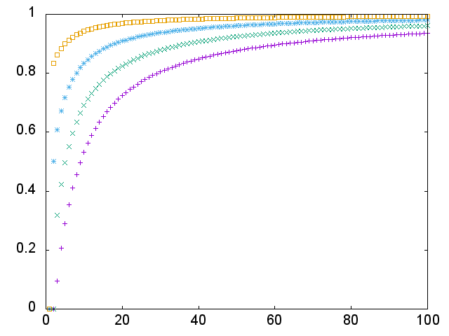
Figure 56: A plot of $R_{n,k}$ for various values of $n$ and $k$ indicating $\lim_{n\to\infty}R_{n,k}=1.$

The proof of Lemma 3.72 is quite involved and is given in Appendix C. Instead, we offer a rough estimate analysis via averaging. The average value of $l_{n}$ is

$$\mathrm{avg}(l_{n}):=\cfrac{\sum_{i=1}^{2n-1}l_{n}(i)}{2n-1}=\frac{n^{2}}{2n-1}.$$ (3.75)

Hence, to a good approximation for large $n$ and small $k,$

$$\begin{split}S_{n,k}&\approxeq\sum_{2n-1\geq i_{k}>i_{k-1}>\cdots>i_{1}\geq 1}[\mathrm{avg}(l_{n})]^{k}\\ &=\left(\frac{n^{2}}{2n-1}\right)^{k}\binom{2n-1}{k}\\ &=\frac{n^{2k}(2n-1)(2n-2)\cdots(2n-k)}{k!(2n-1)^{k}},\end{split}$$ (3.76)

where the second line comes from the fact that there are $\binom{2n-1}{k}$ terms in the summation. Hence, to a good approximation

$$\begin{split}R_{n,k}&\approxeq\frac{n^{2k}(2n-1)(2n-2)\cdots(2n-k)}{(2n-1)^{k}n^{2}(n^{2}-1)\cdots(n^{2}-(k-1))}\\ &=\frac{\left(1-\frac{1}{2n}\right)\cdots\left(1-\frac{k}{2n}\right)}{\left(1-\frac{1}{2n}\right)^{k}\left(1-\frac{1}{n^{2}}\right)\cdots\left(1-\frac{k-1}{n^{2}}\right)}\end{split}$$ (3.77)

Since $k$ is fixed, the right-hand-side tends to $1$ as $n\to\infty.$ Again, the precise proof is given in Appendix C.

Theorem 3.78.

Let ${{\mathrm{triv}}}_{n}$ be the generalization of the expression given in (3.43) for an $n\times n$ grid decomposition. Let ${{\mathrm{triv}}}^{\mathrm{red}}_{n}$ be the same expression but with all terms in which $B$ occurs at least twice at the same height removed. For any $\epsilon>0,$ there exists an $N\in{{\mathbb{N}}}$ such that

$$\left\lVert{{\mathrm{triv}}}_{n}-{{\mathrm{triv}}}_{n}^{\mathrm{red}}\right\rVert\leq\epsilon$$ (3.79)

for all $n\geq N.$

Proof.

Let $M$ be the maximum value of the norms of all quantities of the form $\alpha_{a_{56}^{s}a_{46}^{s}a_{36}^{s}a_{35}^{t}a_{25}^{s}}(B_{14}).$ The difference ${{\mathrm{triv}}}_{n}-{{\mathrm{triv}}}_{n}^{\mathrm{red}}$ only consists of contributions from terms in which there exist at least two $B$’s that occur at the same height. Fix $\epsilon>0.$ To begin, let $K$ be large enough so that

$$\sum_{k=K+1}^{\infty}\frac{M^{k}}{k!}\leq\frac{\epsilon}{2},$$ (3.80)

which is possible since the series for the exponential converges. Furthermore, by Lemma 3.72, for any $\epsilon>0,$ there exists an $N$ large enough so that

$$1-R_{n,k}\leq\frac{\epsilon}{2e^{M}}\quad\forall\;k\leq K,n\geq N.$$ (3.81)

Using these two results, the value of the norm of the difference ${{\mathrm{triv}}}_{n}-{{\mathrm{triv}}}_{n}^{\mathrm{red}}$ is bounded by

$$\begin{split}\left\lVert{{\mathrm{triv}}}_{n}-{{\mathrm{triv}}}_{n}^{\mathrm{red}}\right\rVert&\leq\sum_{k=1}^{n^{2}}\left(\frac{M}{n^{2}}\right)^{k}\left[\binom{n^{2}}{k}-S_{n,k}\right]=\sum_{k=1}^{n^{2}}\left(\frac{M}{n^{2}}\right)^{k}\binom{n^{2}}{k}[1-R_{n,k}]\\ &\leq\sum_{k=1}^{n^{2}}\frac{M^{k}}{k!}[1-R_{n,k}]=\sum_{k=1}^{K}\frac{M^{k}}{k!}[1-R_{n,k}]+\sum_{k=K+1}^{n^{2}}\frac{M^{k}}{k!}[1-R_{n,k}]\\ &\leq\sum_{k=1}^{K}\frac{M^{k}}{k!}\left(\frac{\epsilon}{2e^{M}}\right)+\sum_{k=K+1}^{n^{2}}\frac{M^{k}}{k!}\\ &\leq\left(\frac{\epsilon}{2e^{M}}\right)\sum_{k=1}^{\infty}\frac{M^{k}}{k!}+\sum_{k=K+1}^{\infty}\frac{M^{k}}{k!}\\ &\leq\frac{\epsilon}{2}+\frac{\epsilon}{2}=\epsilon.\end{split}$$ (3.82)

∎

Thus, heuristically, as $n\to\infty,$ the number of terms for which at least two $B$’s are at the same height is a set of measure zero with respect to all possibilities and hence we can ignore them in the calculation of the surface ordered parallel transport after taking the $n\to\infty$ limit. This gives the following picture for the surface-iterated integral. Let $\gamma_{s,t}$ be the (thin) path

The limit of the expression (3.52) as $n\to\infty$ is therefore given by a sum of iterated integrals

$\displaystyle+\int$ $\displaystyle+\int\int$ $+\cdots$

with path-ordering only in the vertical direction. In more detail, the surface-ordered integral is depicted schematically as an infinite sum of terms expressed by placing $B$ at the endpoints of the drawn paths and conjugating it by parallel transport along the path connecting to it using $A$ and $\alpha.$ Then we use an ordinary integral over the horizontal direction to get a 1-form (similar to what is done in [BS] and [SW2]). Finally we use the usual path-ordered integral in the vertical direction. More explicitly, by changing coordinates to

$$u:=\frac{s+t}{\sqrt{2}}\qquad\&\qquad v:=\frac{s-t}{\sqrt{2}},$$ (3.83)

one can express $\gamma_{s,t}$ in terms of $u$ and $v.$ We write this path as $\gamma_{u,v}.$ Using this, the surface parallel transport is given by

$$\begin{split}1&+\int\left(\int\underline{\alpha_{{{\mathrm{triv}}}(\gamma_{u,v})}}\big{(}B(u,v)\big{)}dv\right)du\\ &+\int_{u_{2}\geq u_{1}}\left(\int\underline{\alpha_{{{\mathrm{triv}}}(\gamma_{u_{2},v_{2}})}}\big{(}B(u_{2},v_{2})\big{)}\underline{\alpha_{{{\mathrm{triv}}}(\gamma_{u_{1},v_{1}})}}\big{(}B(u_{1},v_{1})\big{)}dv_{2}dv_{1}\right)du_{2}du_{1}+\cdots\\ &+\int_{u_{n}\geq\cdots\geq u_{1}}\left(\int\underline{\alpha_{{{\mathrm{triv}}}(\gamma_{u_{n},v_{n}})}}\big{(}B(u_{n},v_{n})\big{)}\cdots\underline{\alpha_{{{\mathrm{triv}}}(\gamma_{u_{1},v_{1}})}}\big{(}B(u_{1},v_{1})\big{)}dv_{n}\cdots dv_{1}\right)du_{n}\cdots du_{1}\\ &+\cdots,\end{split}$$ (3.84)

where $B(u,v)$ stands for

$$B(u,v):=B\left(\frac{\partial\Sigma}{\partial s},\frac{\partial\Sigma}{\partial t}\right)\Big{|}_{\left(s=\frac{u+v}{\sqrt{2}},t=\frac{u-v}{\sqrt{2}}\right)}.$$ (3.85)

The sum in (3.84) is absolutely convergent by Propositions 3.57 and 3.61 and Theorem 3.78. In other words,

$$\lim_{n\to\infty}{{\mathrm{triv}}}_{n}=\text{(\ref{eq:surfaceiteratedintegral})}.$$ (3.86)

Remark 3.87.

Although our formula for the surface ordered product for parallel transport has a similar form to the one given by Schreiber and Waldorf in their equation (2.27) of [SW2], they do not look equal. Here, we provide an argument that shows our two formulas are equal. This fact will follow from the defining properties of a crossed module. In terms of bigons, the following figure depicts the differences between the conventions of defining the surface ordered product

for a bigon $\Sigma:\gamma\Rightarrow\delta$ between paths $\gamma,\delta:x\to y.$ The left bigon depicts our automatic ordering that was derived directly from 2-group multiplication with the red quantity appearing to the right of the blue quantity, i.e.

$${\color[rgb]{0,0,1}\underline{\alpha_{{{\mathrm{triv}}}(\beta^{\prime})}}(B^{\prime})}{\color[rgb]{1,0,0}\underline{\alpha_{{{\mathrm{triv}}}(\beta)}}(B)}.$$ (3.88)

The right bigon depicts the ordering convention chosen by [SW2], which can be seen by noting that in their formula, some inverses and minus signs appear that we have avoided. These amount to computing the parallel transport on the leftover form, which they call $\mathcal{A}_{\Sigma},$ along the reverse direction. Also notice that the path they use to act on the $B$ field via the $\alpha$ action from the crossed module actually goes around quite differently than ours. For them, the order is swapped and the expression is written as

$${\color[rgb]{0,0,1}\underline{\alpha_{{{\mathrm{triv}}}(\gamma\tilde{\beta})}}(B)}{\color[rgb]{1,0,0}\underline{\alpha_{{{\mathrm{triv}}}(\gamma\tilde{\beta}^{\prime})}}(B^{\prime})}.$$ (3.89)

Term-by-term, these expressions are in fact different. However, when they are combined and all terms are taken to account in computing the full parallel transport, the resulting 2-group elements describing the parallel transport are the same so that our formulas agree. To see this, we will compare what happens in both of our conventions if we add on an infinitesimal square to an already computed surface transport (cf. (3.32)). Fix $(s,t)\in[0,1]\times[0,1]$ and consider a bigon whose parallel transport has been computed up to $s$ and an additional bigon is to be added at this point

(3.90)

Set

$$\begin{split}h:={{\mathrm{triv}}}(\Sigma_{s}),\quad g_{P}:={{\mathrm{triv}}}(\gamma^{P}_{s,t}),\quad g_{SW}:={{\mathrm{triv}}}(\gamma^{SW}_{s,t}),\\ g:={{\mathrm{triv}}}(\gamma),\quad h_{\Delta}:={{\mathrm{triv}}}(\Delta\Sigma),\quad g_{1}:={{\mathrm{triv}}}(\gamma_{1}).\end{split}$$ (3.91)

Our convention is that the resulting parallel transport of adding this extra piece is given by $\alpha_{g_{P}}(h_{\Delta})h,$ whereas Schreiber and Waldorf’s convention (due to the inverses appearing in their formulas) would give $h\alpha_{gg_{SW}^{-1}}(h_{\Delta}).$ To better compare these, notice that $\tau(h)g=g_{P}g_{1}g_{SW},$ which is equivalent to $gg_{SW}^{-1}=\tau(h^{-1})g_{P}g_{1}.$ Hence,

$$h\alpha_{gg_{SW}^{-1}}(h_{\Delta})=h\alpha_{\tau(h^{-1})g_{P}g_{1}}(h_{\Delta})=\alpha_{g_{P}}(h_{\Delta})h$$ (3.92)

by the properties of crossed module multiplication. Now, by continuity of ${{\mathrm{triv}}},$ these actions, and the group multiplications and since $\displaystyle\lim_{\epsilon\to 0}g_{1}=e,$ the identity element in the group $G,$ we have

$$\lim_{\epsilon\to 0}\big{(}\alpha_{g_{P}}(h_{\Delta})h\big{)}=h\alpha_{gg_{SW}^{-1}}(h_{\Delta})$$ (3.93)

so that our formulas for the parallel transport along surfaces agree.

3.3 Gauge transformations for surface transport

In Section 3.1, we described gauge transformations as natural transformations of parallel transport functors for paths. In this section, we will use this as the definition of a gauge transformation and derive the corresponding formulas for differential forms. As before, let $\mathcal{G}:=(H,G,\tau,\alpha)$ be a crossed module, ${{\mathbb{B}}}\mathcal{G}$ its associated 2-group, and $M$ a smooth manifold. A (first order) gauge transformation from a parallel transport functor ${{\mathrm{triv}}}:\mathcal{P}^{2}M\to{{\mathbb{B}}}\mathcal{G}$ to another ${{\mathrm{triv}}}^{\prime}:\mathcal{P}^{2}(M)\to{{\mathbb{B}}}\mathcal{G}$ is a natural transformation ${{\mathrm{triv}}}\Rightarrow{{\mathrm{triv}}}^{\prime}.$ By Definition 2.25 and Proposition 2.52, such a natural transformation consists of a pair of functions $g:M\to G$ and $h:P^{1}M\to H$ satisfying the conditions described in that Proposition. Namely, to every thin path $z\xleftarrow{\gamma}y,$

$$\tau\big{(}h(\gamma)\big{)}g(z){{\mathrm{triv}}}(\gamma)={{\mathrm{triv}}}^{\prime}(\gamma)g(y),$$ (3.94)

to ever pair of composable thin paths $z\xleftarrow{\gamma}y\xleftarrow{\delta}x,$

$$h(\gamma\delta)=\alpha_{{{\mathrm{triv}}}^{\prime}(\gamma)}\big{(}h(\delta)\big{)}h(\gamma),$$ (3.95)

to every point $x\in M,$

$$h(\mathrm{id}_{x})=e,$$ (3.96)

and finally to any worldsheet

viewed as a bigon from $\gamma\delta$ to $\zeta\xi,$ the equality

=

holds. Reading this diagram is a bit tricky without the arrows (recall Remark 2.13). More explicitly, this equality says

i.e.

$$\alpha_{{{\mathrm{triv}}}^{\prime}(\zeta)}\big{(}h(\xi)\big{)}h(\zeta)\alpha_{g(z)}\big{(}{{\mathrm{triv}}}(\Sigma)\big{)}={{\mathrm{triv}}}^{\prime}(\Sigma)\alpha_{{{\mathrm{triv}}}^{\prime}(\gamma)}\big{(}h(\delta)\big{)}h(\gamma)$$ (3.97)

or equivalently by our earlier condition (3.95)

$$h(\zeta\xi)\alpha_{g(z)}\big{(}{{\mathrm{triv}}}(\Sigma)\big{)}={{\mathrm{triv}}}^{\prime}(\Sigma)h(\gamma\delta).$$ (3.98)

By Proposition 2.52, such a natural transformation can be decomposed into

$$(g,h)=\begin{matrix}[0.9](g,e)\\ (e,h)\end{matrix}.$$ (3.99)

A gauge transformation of the type $(g,e)$ is typically called a (first order) thin gauge transformation and one of the type $(e,h)$ is called a (first order) fat gauge transformation [MM]. Thus, Proposition 2.52 implies that an arbitrary gauge transformation of the first kind can be decomposed into a thin and fat gauge transformation. Using this, we can calculate infinitesimal versions of the functions $g:M\to G$ and $h:P^{1}M\to H$ for small paths, i.e. for a point $x\in M$ and a tangent vector at $x.$ This was already done for $g:M\to G$ at the end of Section 3.1 with result (3.17). For $h:P^{1}M\to H,$ let $t\mapsto x(t)$ parametrize an infinitesimal path $\gamma,$ then to lowest order in $\Delta t$

$$h(\gamma)=\exp\left\{\varphi_{\mu}\big{(}x(t)\big{)}\frac{dx^{\mu}}{dt}\Big{|}_{t}\Delta t\right\}$$ (3.100)

for some 1-form $\varphi\in\Omega^{1}(M;\mathfrak{h}).$ Thus, plugging these expressions into (3.94), a fat gauge transformation from $(A,B)$ to $(A^{\prime},B^{\prime})$ infinitesimally gives

$$\tau\left(\exp\left\{\varphi_{\mu}\big{(}x(t)\big{)}\frac{dx^{\mu}}{dt}\Big{|}_{t}\Delta t\right\}\right)\exp\left\{-A_{\nu}\big{(}x(t)\big{)}\frac{dx^{\nu}}{dt}\Big{|}_{t}\Delta t\right\}=\exp\left\{-A^{\prime}_{\nu}\big{(}x(t)\big{)}\frac{dx^{\nu}}{dt}\Big{|}_{t}\Delta t\right\}$$ (3.101)

because $g$ has been set to be the identity. Expanding out to lowest order in $\Delta t$ gives

$$\mathds{1}+\underline{\tau}\left(\varphi_{\mu}\big{(}x(t)\big{)}\frac{dx^{\mu}}{dt}\Big{|}_{t}\right)\Delta t-A_{\nu}\big{(}x(t)\big{)}\frac{dx^{\nu}}{dt}\Big{|}_{t}\Delta t=\mathds{1}-A^{\prime}_{\nu}\big{(}x(t)\big{)}\frac{dx^{\nu}}{dt}\Big{|}_{t}\Delta t$$ (3.102)

giving the relationship

$$A^{\prime}=A-\underline{\tau}(\varphi)$$ (3.103)

for a fat gauge transformation. We already calculated what happens for a thin gauge transformation in Section 3.1. Using Proposition 2.52, combining (3.17) with this gives

$$A^{\prime}=gAg^{-1}-dgg^{-1}-\underline{\tau}(\varphi)$$ (3.104)

for an arbitrary gauge transformation. The $B$ field under an arbitrary gauge transformation changes according to (3.97). By substituting the necessary forms, this expression on the left-hand-side of (3.97) becomes (to avoid clutter, we have not explicitly written $\Delta s$ and $\Delta t$)

$$\begin{split}&\alpha_{\exp\left\{-A^{\prime}_{\nu}\big{(}x(s,t+\epsilon)\big{)}\frac{\partial x^{\nu}}{\partial s}\Big{|}_{(s,t+\epsilon)}\right\}}\left(\exp\left\{\varphi_{\mu}\big{(}x(s,t)\big{)}\frac{\partial x^{\mu}}{\partial t}\Big{|}_{(s,t)}\right\}\right)\\ &\quad\times\exp\left\{\varphi_{\rho}\big{(}x(s,t+\epsilon)\big{)}\frac{\partial x^{\rho}}{\partial s}\Big{|}_{(s,t+\epsilon)}\right\}\alpha_{g(x(s+\epsilon,t+\epsilon))}\left(\exp\left\{B_{\sigma\tau}\big{(}x(s,t)\big{)}\frac{\partial x^{\sigma}}{\partial s}\frac{\partial x^{\tau}}{\partial t}\Big{|}_{(s,t)}\right\}\right)\\ &=\alpha_{\mathds{1}-A^{\prime}_{\nu}\frac{\partial x^{\nu}}{\partial s}-\frac{\partial A^{\prime}_{\nu}}{\partial x^{\lambda}}\frac{\partial x^{\lambda}}{\partial t}\frac{\partial x^{\nu}}{\partial s}-A^{\prime}_{\nu}\frac{\partial^{2}x^{\nu}}{\partial s\partial t}}\left(\mathds{1}+\varphi_{\mu}\frac{\partial x^{\mu}}{\partial t}\right)\\ &\quad\times\left(\mathds{1}+\varphi_{\rho}\frac{\partial x^{\rho}}{\partial s}+\frac{\partial\varphi_{\rho}}{\partial x^{\beta}}\frac{\partial x^{\beta}}{\partial t}\frac{\partial x^{\rho}}{\partial s}+\varphi_{\rho}\frac{\partial^{2}x^{\rho}}{\partial s\partial t}\right)\alpha_{g+\frac{\partial g}{\partial s}+\frac{\partial g}{\partial t}+\frac{\partial^{2}g}{\partial s\partial t}}\left(\mathds{1}+B_{\sigma\tau}\frac{\partial x^{\sigma}}{\partial s}\frac{\partial x^{\tau}}{\partial t}\right)\\ &=\mathds{1}+\varphi_{\mu}\varphi_{\rho}\frac{\partial x^{\mu}}{\partial t}\frac{\partial x^{\rho}}{\partial s}+\frac{\partial\varphi_{\rho}}{\partial x^{\beta}}\frac{\partial x^{\beta}}{\partial t}\frac{\partial x^{\rho}}{\partial s}+\varphi_{\rho}\frac{\partial^{2}x^{\rho}}{\partial s\partial t}+\underline{\alpha_{g}}(B_{\sigma\tau})\frac{\partial x^{\sigma}}{\partial s}\frac{\partial x^{\tau}}{\partial t}-\underline{\alpha}_{A^{\prime}_{\nu}}(\varphi_{\mu})\frac{\partial x^{\nu}}{\partial s}\frac{\partial x^{\mu}}{\partial t}\\ &=\mathds{1}+\varphi_{\lambda}\frac{\partial^{2}x^{\lambda}}{\partial s\partial t}+\left(\varphi_{\nu}\varphi_{\mu}+\frac{\partial\varphi_{\mu}}{\partial x^{\nu}}+\underline{\alpha_{g}}(B_{\mu\nu})-\underline{\alpha}_{A^{\prime}_{\mu}}(\varphi_{\nu})\right)\frac{\partial x^{\mu}}{\partial s}\frac{\partial x^{\nu}}{\partial t},\end{split}$$ (3.105)

where it is understood that all terms now are evaluated at $(s,t),$ to lowest order. Meanwhile, the right-hand-side of (3.97) is

$$\begin{split}&\exp\left\{B^{\prime}_{\sigma\tau}\big{(}x(s,t)\big{)}\frac{\partial x^{\sigma}}{\partial s}\frac{\partial x^{\tau}}{\partial t}\Big{|}_{(s,t)}\right\}\alpha_{\exp\left\{-A^{\prime}_{\nu}\big{(}x(s+\epsilon,t)\big{)}\frac{\partial x^{\nu}}{\partial t}\Big{|}_{(s+\epsilon,t)}\right\}}\left(\exp\left\{\varphi_{\mu}\big{(}x(s,t)\big{)}\frac{\partial x^{\mu}}{\partial s}\Big{|}_{(s,t)}\right\}\right)\\ &\quad\times\exp\left\{\varphi_{\lambda}\big{(}x(s+\epsilon,t)\big{)}\frac{\partial x^{\lambda}}{\partial t}\Big{|}_{(s+\epsilon,t)}\right\}\\ &=\left(\mathds{1}+B^{\prime}_{\sigma\tau}\frac{\partial x^{\sigma}}{\partial s}\frac{\partial x^{\tau}}{\partial t}\right)\alpha_{\mathds{1}-A^{\prime}_{\nu}\frac{\partial x^{\nu}}{\partial t}-\frac{\partial A^{\prime}_{\nu}}{\partial x^{\beta}}\frac{\partial x^{\beta}}{\partial s}\frac{\partial x^{\nu}}{\partial t}-A^{\prime}_{\nu}\frac{\partial^{2}x^{\nu}}{\partial t\partial s}}\left(\mathds{1}+\varphi_{\mu}\frac{\partial x^{\mu}}{\partial s}\right)\\ &\quad\times\left(\mathds{1}+\varphi_{\lambda}\frac{\partial x^{\lambda}}{\partial t}+\frac{\partial\varphi_{\lambda}}{\partial x^{\alpha}}\frac{\partial x^{\alpha}}{\partial s}\frac{\partial x^{\lambda}}{\partial t}+\varphi_{\lambda}\frac{\partial^{2}x^{\lambda}}{\partial t\partial s}\right)\\ &=\mathds{1}+B^{\prime}_{\sigma\tau}\frac{\partial x^{\sigma}}{\partial s}\frac{\partial x^{\tau}}{\partial t}+\varphi_{\mu}\varphi_{\lambda}\frac{\partial x^{\mu}}{\partial s}\frac{\partial x^{\lambda}}{\partial t}-\underline{\alpha}_{A^{\prime}_{\nu}}(\varphi_{\mu})\frac{\partial x^{\nu}}{\partial t}\frac{\partial x^{\mu}}{\partial s}+\frac{\partial\varphi_{\lambda}}{\partial x^{\alpha}}\frac{\partial x^{\alpha}}{\partial s}\frac{\partial x^{\lambda}}{\partial t}+\varphi_{\lambda}\frac{\partial^{2}x^{\lambda}}{\partial t\partial s}\\ &=\mathds{1}+\varphi_{\lambda}\frac{\partial^{2}x^{\lambda}}{\partial t\partial s}+\left(\varphi_{\mu}\varphi_{\nu}+B^{\prime}_{\mu\nu}-\underline{\alpha}_{A^{\prime}_{\nu}}(\varphi_{\mu})+\frac{\partial\varphi_{\nu}}{\partial x^{\mu}}\right)\frac{\partial x^{\mu}}{\partial s}\frac{\partial x^{\nu}}{\partial t}\end{split}$$ (3.106)

again to lowest order. Equating these two expressions gives

$$B^{\prime}_{\mu\nu}=\underline{\alpha_{g}}(B_{\mu\nu})-\varphi_{\mu}\varphi_{\nu}-\varphi_{\nu}\varphi_{\mu}-\partial_{\mu}\varphi_{\nu}-\partial_{\nu}\varphi_{\mu}-\underline{\alpha}_{A^{\prime}_{\mu}}(\varphi_{\nu})+\underline{\alpha}_{A^{\prime}_{\nu}}(\varphi_{\mu})$$ (3.107)

in components or

$$B^{\prime}=\underline{\alpha_{g}}(B)-\varphi\wedge\varphi-d\varphi-\underline{\alpha}_{A^{\prime}}(\varphi)$$ (3.108)

as an equation in terms of differential forms. We write such a gauge transformation as

$$(A,B)\xrightarrow{(g,\varphi)}(A^{\prime},B^{\prime}).$$ (3.109)

This and (3.104) agrees with Proposition 2.10 of [SW2]. We can express this purely in terms of $A,$ $B,$ $g,$ and $\varphi$ as

$$\begin{split}B^{\prime}&=\underline{\alpha_{g}}(B)-\varphi\wedge\varphi-d\varphi-\underline{\alpha}_{gAg^{-1}-dgg^{-1}-\underline{\tau}(\varphi)}(\varphi)\\ &=\underline{\alpha_{g}}(B)-\varphi\wedge\varphi-d\varphi-\underline{\alpha}_{gAg^{-1}-dgg^{-1}}(\varphi)+[\varphi,\varphi]\\ &=\underline{\alpha_{g}}(B)+\varphi\wedge\varphi-d\varphi-\underline{\alpha}_{gAg^{-1}-dgg^{-1}}(\varphi).\end{split}$$ (3.110)

This will be useful later.

Now suppose $(g,h),(g^{\prime},h^{\prime}):{{\mathrm{triv}}}\Rightarrow{{\mathrm{triv}}}^{\prime}$ are two first order gauge transformations. A second order gauge transformation $a:(g,h)\Rrightarrow(g^{\prime},h^{\prime})$ is a modification from $(g,h)$ to $(g^{\prime},h^{\prime}).$ By Definition 2.34, this consists of a function $a:M\to H$ fitting into

,

which in particular says

$$\tau(a)g=g^{\prime},$$ (3.111)

satisfying the condition that to any path $y\xleftarrow{\gamma}x,$

$$h^{\prime}(\gamma)a(y)=\alpha_{{{\mathrm{triv}}}^{\prime}(\gamma)}\big{(}a(x)\big{)}h(\gamma).$$ (3.112)

Expanding out this expression on infinitesimal paths gives

$$\left(\mathds{1}+\varphi^{\prime}_{\mu}\frac{dx^{\mu}}{dt}\right)\left(a+\frac{\partial a}{\partial x^{\nu}}\frac{dx^{\nu}}{dt}\right)=\alpha_{\mathds{1}-A^{\prime}_{\mu}\frac{dx^{\mu}}{dt}}(a)\left(\mathds{1}+\varphi_{\nu}\frac{dx^{\nu}}{dt}\right),$$ (3.113)

which to lowest order says

$$\mathds{1}+\varphi^{\prime}_{\mu}a\frac{dx^{\mu}}{dt}+\frac{\partial a}{\partial x^{\nu}}\frac{dx^{\nu}}{dt}=\mathds{1}+a\varphi_{\nu}\frac{dx^{\nu}}{dt}-\underline{\alpha_{a}}(A^{\prime}_{\mu})\frac{dx^{\mu}}{dt}.$$ (3.114)

Note that if $h\in H,$ the function $\alpha_{h}:G\to H$ is defined by $G\ni g\mapsto\alpha_{g}(h)$ so that $\underline{\alpha_{h}}:\mathfrak{g}\to\mathfrak{h}$ is the derivative. This result gives the condition (after multiplying by $a^{-1}$ on the right)

$$\varphi^{\prime}_{\mu}=a\varphi_{\mu}a^{-1}-\underline{\alpha_{a}}(A^{\prime}_{\mu})a^{-1}-(\partial_{\mu}a)a^{-1}$$ (3.115)

on components and

$$\varphi^{\prime}=a\varphi a^{-1}-daa^{-1}-\underline{\alpha_{a}}(A^{\prime})a^{-1}$$ (3.116)

as $\mathfrak{h}$-valued differential forms. This and (3.111) exactly agree with Proposition 2.11 of [SW2]. Physically, a second order gauge transformation is a gauge transformation for the 1-form $\varphi,$ which itself is a type of field even though it appears as a (fat) gauge transformation for the 1-form and 2-form gauge potentials.

3.4 Orientations and inverses

It is well-known that given a path $y\xleftarrow{\gamma}x,$ the parallel transport along the reversed oriented path $\gamma^{-1}$ is the inverse

$${{\mathrm{triv}}}(\gamma^{-1})={{\mathrm{triv}}}(\gamma)^{-1},$$ (3.117)

where ${{\mathrm{triv}}}:\mathcal{P}^{1}M\to{{\mathbb{B}}}G$ is the (local) parallel transport functor. This can be viewed as a consequence of thin homotopy invariance and functoriality of parallel transport. Namely, although the paths $\gamma\gamma^{-1}$ and $\gamma^{-1}\gamma$ are not the constant paths (the notation $\gamma^{-1}$ is therefore a bit abusive), they are thinly homotopic to constant paths and hence give the same value on ${{\mathrm{triv}}}.$ Thus,

(3.118)

verifying (3.117). In this section, we will explore analogous results for reversing different kinds of orientations on bigons. We therefore include arrows for clarity.

Technically, there is one more possibility given by $\underline{\Sigma}:\delta^{-1}\Rightarrow\gamma^{-1}.$ However, this possibility is a combination of the above two, namely $\underline{\Sigma}=\overline{\Sigma^{-1}}.$ The meaning of these different possibilities is given physically as follows. A given string may be given the additional datum of an orientation. Furthermore, as it moves in time, it has an additional directionality. These two directional orientations are precisely encoded in the definition of a bigon/2-morphism. These different orientation reversals are given by time reversal for $\overline{\Sigma}$ and spatial orientation reversal for $\Sigma^{-1}.$ The case $\underline{\Sigma}$ corresponds to both reversals (the order of reversal does not matter since the operations commute). Note that the different orientations on a bigon can be expressed as an orientation of edges on the boundary and an orientation of the surface. The above bigons correspond to the following surfaces with associated orientations

respectively.

A necessary and sufficient condition for such orientations on surfaces and edges to give rise to a bigon is the following. Given a map of a polygon $\Sigma$ into $M,$ the boundary consists of the edges of the polygon. The union of the oriented edges consistent with the orientation of the polygon must be connected. Similarly, the union of the orientated edges with negative orientation with respect to the induced one from the polygon must also be connected. Then, the source of the bigon is the union of the consistent edges and the target is the union of the oppositely oriented edges. An example together with a non-example are

& ,

respectively (blue, with arrows written using $>,$ corresponds to an orientation agreeing with the induced one from the surface while yellow, with arrows written using $\gg,$ disagrees with that orientation).

Going back to the three bigons and their orientations at the beginning of this section, we notice that several of these bigons can be composed with one another. For instance,

and

after applying thin homotopies. Therefore, these bigons provide inverses in series and in parallel, respectively, of $\Sigma.$ This implies, together with functoriality of ${{\mathrm{triv}}}$ and the inverses discussed in Example 2.45,

$${{\mathrm{triv}}}\big{(}\overline{\Sigma}\big{)}={{\mathrm{triv}}}(\Sigma)^{-1}\qquad\&\qquad{{\mathrm{triv}}}\big{(}\Sigma^{-1}\big{)}=\alpha_{{{\mathrm{triv}}}(\gamma)^{-1}}\big{(}{{\mathrm{triv}}}(\Sigma)^{-1}\big{)}$$ (3.119)

and therefore describes how parallel transport along surfaces changes under reversals in surface orientations and boundary orientations, respectively. For completeness, for the last possible orientation $\underline{\Sigma}:\delta^{-1}\Rightarrow\gamma^{-1},$ we have

$${{\mathrm{triv}}}\left(\underline{\Sigma}\right)={{\mathrm{triv}}}\left(\overline{\Sigma^{-1}}\right)=\left(\alpha_{{{\mathrm{triv}}}(\gamma)^{-1}}\big{(}{{\mathrm{triv}}}(\Sigma)\big{)}^{-1}\right)^{-1}=\alpha_{{{\mathrm{triv}}}(\gamma)^{-1}}\big{(}{{\mathrm{triv}}}(\Sigma)\big{)}.$$ (3.120)

3.5 The 3-curvature

In the following, we make some further calculations. Just as the curvature $F$ of a 1-form connection $A$ can be obtained by calculating the parallel transport along an infinitesimal loop, the 2-curvature of a 2-form connection $(A,B)$ can be obtained by calculating the surface transport along an infinitesimal sphere, which on a lattice corresponds to a cube. We will perform this calculation explicitly and study some properties of the resulting 3-form curvature. Similar analysis was done on a tetrahedron in [GP].

Let $(r,s,t)\mapsto x(r,s,t)$ be an infinitesimal cube and consider the following domain for that cube along with the infinitesimal path that goes first along the $r$ direction, then in the $s$ direction, and finally in the $t$ direct. Our convention is that $(r,s,t)$ is a right-handed coordinate frame, i.e. $dr\wedge ds\wedge dt$ is the volume form.

Such a cube can be expressed as a bigon by the following composition of plaquette bigons that begin and end at the same path starting at the top left and moving clockwise.

$\rightsquigarrow$ $\rightsquigarrow$

$\rightsquigarrow$

$\rightsquigarrow$

The corresponding 2-group elements are given as follows. We begin with the first surface

$\leftrightarrow$

where we use the shorthand notation

$$\partial_{r}x:=\frac{\partial x}{\partial r},\qquad\partial_{s}x:=\frac{\partial x}{\partial s},\qquad\&\qquad\partial_{t}x:=\frac{\partial x}{\partial t}$$ (3.121)

as well as

$$e^{-A_{\mu}\partial_{t}x^{\mu}|_{(\epsilon,\epsilon,0)}}:=\exp\left\{-A_{\mu}\big{(}x(\epsilon,\epsilon,0)\big{)}\frac{\partial x^{\mu}}{\partial t}\Big{|}_{(\epsilon,\epsilon,0)}\right\}$$ (3.122)

and similarly for the other terms. We also write $\epsilon$ instead of $\Delta r,\Delta s,$ or $\Delta t$ and use the derivatives to remind ourselves of the direction. We have also assumed for simplicity that our coordinates are centered at the origin and the lattice spacing is $\epsilon$ in each direction. Working out this diagram infinitesimally on the 0-d defect gives

$$\alpha_{e^{-A_{\mu}\partial_{t}x^{\mu}|_{(\epsilon,\epsilon,0)}}}\left(e^{B_{\lambda\nu}\partial_{r}x^{\lambda}\partial_{s}x^{\nu}|_{(0,0,0)}}\right)=\mathds{1}+B_{\lambda\nu}\partial_{r}x^{\lambda}\partial_{s}x^{\nu}-\underline{\alpha}_{A_{\mu}}(B_{\lambda\nu})\partial_{t}x^{\mu}\partial_{r}x^{\lambda}\partial_{s}x^{\nu}$$ (3.123)

to lowest order. As usual, rather than writing out the $\Delta r,\Delta s,\Delta t,$ we use the number and type of derivatives appearing to keep track of the order. The other terms are given by the following

$\leftrightarrow$

$$\begin{split}e^{B_{\rho\pi}\partial_{r}x^{\rho}\partial_{t}x^{\pi}|_{(0,\epsilon,0)}}&=\mathds{1}+B_{\rho\pi}\partial_{r}x^{\rho}\partial_{t}x^{\pi}+\partial_{c}B_{\rho\pi}\partial_{s}x^{c}\partial_{r}x^{\rho}\partial_{t}x^{\pi}\\ &\quad+B_{\rho\pi}\partial_{s}\partial_{r}x^{\rho}\partial_{t}x^{\pi}+B_{\rho\pi}\partial_{r}x^{\rho}\partial_{s}\partial_{t}x^{\pi}\end{split}$$ (3.124)

$\leftrightarrow$

$$\alpha_{e^{-A_{\alpha}\partial_{r}x^{\alpha}|_{(0,0,\epsilon)}}}\left(e^{B_{\sigma\tau}\partial_{s}x^{\sigma}\partial_{t}x^{\tau}|_{(0,0,0)}}\right)=\mathds{1}+B_{\sigma\tau}\partial_{s}x^{\sigma}\partial_{t}x^{\tau}-\underline{\alpha}_{A_{\alpha}}(B_{\sigma\tau})\partial_{r}x^{\alpha}\partial_{s}x^{\sigma}\partial_{t}x^{\tau}$$ (3.125)

$\leftrightarrow$

$$\begin{split}e^{B_{\beta\kappa}\partial_{s}x^{\beta}\partial_{r}x^{\kappa}|_{(0,0,\epsilon)}}&=\mathds{1}+B_{\beta\kappa}\partial_{s}x^{\beta}\partial_{r}x^{\kappa}+\partial_{b}B_{\beta\kappa}\partial_{t}x^{b}\partial_{s}x^{\beta}\partial_{r}x^{\kappa}\\ &\quad+B_{\beta\kappa}\partial_{t}\partial_{s}x^{\beta}\partial_{r}x^{\kappa}+B_{\beta\kappa}\partial_{s}x^{\beta}\partial_{t}\partial_{r}x^{\kappa}\end{split}$$ (3.126)

$\leftrightarrow$

$$\alpha_{e^{-A_{\theta}\partial_{s}x^{\theta}|_{(\epsilon,0,\epsilon)}}}\left(e^{B_{\gamma\eta}\partial_{t}x^{\gamma}\partial_{r}x^{\eta}|_{(0,0,0)}}\right)=\mathds{1}+B_{\gamma\eta}\partial_{t}x^{\gamma}\partial_{r}x^{\eta}-\underline{\alpha}_{A_{\theta}}(B_{\gamma\eta})\partial_{s}x^{\theta}\partial_{t}x^{\gamma}\partial_{r}x^{\eta}$$ (3.127)

$\leftrightarrow$

$$\begin{split}e^{B_{\omega\psi}\partial_{t}x^{\omega}\partial_{s}x^{\psi}|_{(\epsilon,0,0)}}&=\mathds{1}+B_{\omega\psi}\partial_{t}x^{\omega}\partial_{s}x^{\psi}+\partial_{a}B_{\omega\psi}\partial_{r}x^{a}\partial_{t}x^{\omega}\partial_{s}x^{\psi}\\ &\quad+B_{\omega\psi}\partial_{r}\partial_{t}x^{\omega}\partial_{s}x^{\psi}+B_{\omega\psi}\partial_{t}x^{\omega}\partial_{r}\partial_{s}x^{\psi}\end{split}$$ (3.128)

The composition of all of these elements is given by the following diagram (with the light shaded blue squares depicting the faces on the cube).

And the result of multiplying these out gives

$$\begin{split}e^{B_{\omega\psi}\partial_{t}x^{\omega}\partial_{s}x^{\psi}|_{(\epsilon,0,0)}}\alpha_{e^{-A_{\theta}\partial_{s}x^{\theta}|_{(\epsilon,0,\epsilon)}}}\left(e^{B_{\gamma\eta}\partial_{t}x^{\gamma}\partial_{r}x^{\eta}|_{(0,0,0)}}\right)e^{B_{\beta\kappa}\partial_{s}x^{\beta}\partial_{r}x^{\kappa}|_{(0,0,\epsilon)}}\\ \times\alpha_{e^{-A_{\alpha}\partial_{r}x^{\alpha}|_{(0,0,\epsilon)}}}\left(e^{B_{\sigma\tau}\partial_{s}x^{\sigma}\partial_{t}x^{\tau}|_{(0,0,0)}}\right)e^{B_{\rho\pi}\partial_{r}x^{\rho}\partial_{t}x^{\pi}|_{(0,\epsilon,0)}}\alpha_{e^{-A_{\mu}\partial_{t}x^{\mu}|_{(\epsilon,\epsilon,0)}}}\left(e^{B_{\lambda\nu}\partial_{r}x^{\lambda}\partial_{s}x^{\nu}|_{(0,0,0)}}\right).\end{split}$$ (3.129)

This is yet another manifestation of two-dimensional algebra. The result of multiplying all these terms is given as follows, order by order. The zeroth order term is $\mathds{1}.$ There are no first order terms. The second order terms are given by

$$\begin{split}B_{\omega\psi}\partial_{t}x^{\omega}\partial_{s}x^{\psi}&+B_{\gamma\eta}\partial_{t}x^{\gamma}\partial_{r}x^{\eta}+B_{\beta\kappa}\partial_{s}x^{\beta}\partial_{r}x^{\kappa}+B_{\sigma\tau}\partial_{s}x^{\sigma}\partial_{t}x^{\tau}+B_{\rho\pi}\partial_{r}x^{\rho}\partial_{t}x^{\pi}+B_{\lambda\nu}\partial_{r}x^{\lambda}\partial_{s}x^{\nu}\\ &=(B_{\sigma\tau}+B_{\tau\sigma})\partial_{s}x^{\sigma}\partial_{t}x^{\tau}+(B_{\lambda\nu}+B_{\nu\lambda})\partial_{r}x^{\lambda}\partial_{s}x^{\nu}+(B_{\rho\pi}+B_{\pi\rho})\partial_{r}x^{\rho}\partial_{t}x^{\pi}\\ &=0\end{split}$$ (3.130)

by anti-symmetry of $B_{\mu\nu}$ in the $\mu$ and $\nu$ indices. Thus, the only non-zero terms are the zeroth and third order terms (up to third order). One type of the third order terms are given by

$$\begin{split}\Big{(}&B_{\omega\psi}\partial_{r}\partial_{t}x^{\omega}\partial_{s}x^{\psi}+B_{\omega\psi}\partial_{t}x^{\omega}\partial_{r}\partial_{s}x^{\psi}+B_{\beta\kappa}\partial_{t}\partial_{s}x^{\beta}\partial_{r}x^{\kappa}\Big{)}\\ +\Big{(}&B_{\beta\kappa}\partial_{s}x^{\beta}\partial_{t}\partial_{r}x^{\kappa}+B_{\rho\pi}\partial_{s}\partial_{r}x^{\rho}\partial_{t}x^{\pi}+B_{\rho\pi}\partial_{r}x^{\rho}\partial_{s}\partial_{t}x^{\pi}\Big{)}\\ &=(B_{\beta\kappa}+B_{\kappa\beta})\partial_{s}x^{\beta}\partial_{t}\partial_{r}x^{\kappa}+(B_{\omega\psi}+B_{\psi\omega})\partial_{t}x^{\omega}\partial_{r}\partial_{s}x^{\psi}+(B_{\rho\pi}+B_{\pi\rho})\partial_{r}x^{\rho}\partial_{s}\partial_{t}x^{\pi}\end{split}$$ (3.131)

and vanish again by anti-symmetry of $B_{\mu\nu}$ and commutativity of partial derivatives. The final result is therefore

$$\begin{split}\mathds{1}&+\partial_{a}B_{\omega\psi}\partial_{r}x^{a}\partial_{t}x^{\omega}\partial_{s}x^{\psi}-\underline{\alpha}_{A_{\theta}}(B_{\gamma\eta})\partial_{s}x^{\theta}\partial_{t}x^{\gamma}\partial_{r}x^{\eta}+\partial_{b}B_{\beta\kappa}\partial_{t}x^{b}\partial_{s}x^{\beta}\partial_{r}x^{\kappa}\\ &-\underline{\alpha}_{A_{\alpha}}(B_{\sigma\tau})\partial_{r}x^{\alpha}\partial_{s}x^{\sigma}\partial_{t}x^{\tau}+\partial_{c}B_{\rho\pi}\partial_{s}x^{c}\partial_{r}x^{\rho}\partial_{t}x^{\pi}\ -\underline{\alpha}_{A_{\mu}}(B_{\lambda\nu})\partial_{t}x^{\mu}\partial_{r}x^{\lambda}\partial_{s}x^{\nu}\\ &=\mathds{1}-\Big{(}\partial_{\mu}B_{\nu\lambda}+\partial_{\lambda}B_{\mu\nu}+\partial_{\nu}B_{\lambda\mu}+\underline{\alpha}_{A_{\mu}}(B_{\nu\lambda})+\underline{\alpha}_{A_{\nu}}(B_{\lambda\mu})+\underline{\alpha}_{A_{\lambda}}(B_{\mu\nu})\Big{)}\partial_{r}x^{\mu}\partial_{s}x^{\nu}\partial_{t}x^{\lambda}.\end{split}$$ (3.132)

In analogy to the curvature 2-form associated to a 1-form potential $A$ obtained by calculating the holonomy along an infinitesimal square, we define this third order term to be the 3-form curvature associated to the pair $(A,B)$ and denote it by $H.$ In terms of components, it is given by

$$H_{\mu\nu\lambda}:=\partial_{\mu}B_{\nu\lambda}+\partial_{\lambda}B_{\mu\nu}+\partial_{\nu}B_{\lambda\mu}+\underline{\alpha}_{A_{\mu}}(B_{\nu\lambda})+\underline{\alpha}_{A_{\nu}}(B_{\lambda\mu})+\underline{\alpha}_{A_{\lambda}}(B_{\mu\nu})$$ (3.133)

and using differential form notation

$$H:=dB+\underline{\alpha}_{A}(B).$$ (3.134)

This definition and result agrees with (3.28) of [GP] and Lemma A.11 in [SW2]. As was also pointed out in [GP],

$$\underline{\tau}(H)=\underline{\tau}(dB)+\underline{\tau}\big{(}\underline{\alpha}_{A}(B)\big{)}=d\underline{\tau}(B)+[A,\underline{\tau}(B)]=dF+[A,F]=0$$ (3.135)

by the Bianchi identity. Since $\ker\underline{\tau}$ is a central Lie subalgebra of $\mathfrak{h},$ this means $H$ is a 3-form with values in an abelian Lie algebra (see Remark 2.44). Under a first order gauge transformation $(A,B)\xrightarrow{(g,\varphi)}(A^{\prime},B^{\prime})$ as in (3.109) and using (3.110), the 3-form curvature changes to

$$\begin{split}H^{\prime}&=dB^{\prime}+\underline{\alpha}_{A^{\prime}}(B^{\prime})\\ &=d\Big{(}\underline{\alpha_{g}}(B)+\varphi\wedge\varphi-d\varphi-\underline{\alpha}_{gAg^{-1}-dgg^{-1}}(\varphi)\Big{)}\\ &\quad+\underline{\alpha}_{gAg^{-1}-dgg^{-1}-\underline{\tau}(\varphi)}\Big{(}\underline{\alpha_{g}}(B)+\varphi\wedge\varphi-d\varphi-\underline{\alpha}_{gAg^{-1}-dgg^{-1}}(\varphi)\Big{)}\\ &=\underbrace{d\big{(}\underline{\alpha_{g}}(B)\big{)}}_{(\ref{eq:3curvdagB})}+\uwave{d\varphi\wedge\varphi-\varphi\wedge d\varphi}-\underbrace{d\big{(}\underline{\alpha}_{gAg^{-1}-dgg^{-1}}(\varphi)\big{)}}_{(\ref{eq:3curvdaAprimephi})}\\ &\quad+\underbrace{\underline{\alpha}_{gAg^{-1}-dgg^{-1}}\big{(}\underline{\alpha_{g}}(B)\big{)}}_{(\ref{eq:3curvagaAB})}-\underline{\alpha}_{dgg^{-1}}\big{(}\underline{\alpha_{g}}(B)\big{)}+\underbrace{\underline{\alpha}_{gAg^{-1}-dgg^{-1}}\big{(}\varphi\wedge\varphi\big{)}}_{(\ref{eq:3curveaAprimephiphi})}\\ &\quad-\underbrace{\underline{\alpha}_{gAg^{-1}-dgg^{-1}}\big{(}\underline{\alpha}_{gAg^{-1}-dgg^{-1}}(\varphi)\big{)}}_{(\ref{eq:3curvaAprimeaAprimephi})}-\underbrace{\underline{\alpha}_{gAg^{-1}-dgg^{-1}}(d\varphi)}_{(\ref{eq:3curvdaAprimephi})}\\ &\quad-[\varphi,\underline{\alpha_{g}}(B)]-\underbrace{[\varphi,\varphi\wedge\varphi]}_{0}+\uwave{[\varphi,d\varphi]}+[\varphi,\underline{\alpha}_{gAg^{-1}-dgg^{-1}}(\varphi)],\end{split}$$ (3.136)

where the underlined terms cancel and the other terms with underbraces will be calculated and compared momentarily. At this point, it is useful to simplify some of these terms by applying $\underline{\tau}$ and calculating the results in terms of commutators and such. For example,

$$\begin{split}\underline{\tau}\Big{(}d\underline{\alpha_{g}}(B)\big{)}\Big{)}&=d\Big{(}\underline{\tau}\big{(}\underline{\alpha_{g}}(B)\big{)}\Big{)}\\ &=d\big{(}g\underline{\tau}(B)g^{-1}\big{)}\\ &=dg\underline{\tau}(B)g^{-1}+g\underline{\tau}(dB)g^{-1}+g\underline{\tau}(B)dg^{-1}\\ &=dgg^{-1}g\underline{\tau}(B)g^{-1}+\underline{\tau}\big{(}\underline{\alpha_{g}}(dB)\big{)}-g\underline{\tau}(B)g^{-1}dgg^{-1}\\ &=\underline{\tau}\Big{(}\underline{\alpha_{g}}(dB)+\underline{\alpha}_{dgg^{-1}}\big{(}\underline{\alpha_{g}}(B)\big{)}\Big{)}.\end{split}$$ (3.137)

We can safely equate the terms inside the $\underline{\tau}.$ This is a helpful trick and we will use it to calculate all other terms. For instance, one can show using this trick that

$$\underline{\alpha}_{gAg^{-1}}\big{(}\underline{\alpha_{g}}(B)\big{)}=\underline{\alpha_{g}}\big{(}\underline{\alpha}_{A}(B)\big{)}.$$ (3.138)

Although this is a trick and not completely rigorous, it works for all of the calculations we will do. These formulas can all be found in Appendix A of [Wal1] and can be derived more rigorously. Since $\underline{\alpha}$ is a derivation,

$$\underline{\alpha}_{gAg^{-1}-dgg^{-1}}(\varphi\wedge\varphi)=\underline{\alpha}_{gAg^{-1}-dgg^{-1}}(\varphi)\wedge\varphi-\varphi\wedge\underline{\alpha}_{gAg^{-1}-dgg^{-1}}(\varphi),$$ (3.139)

which cancels with the term $[\varphi,\underline{\alpha}_{gAg^{-1}-dgg^{-1}}(\varphi)]$ in (3.136). Furthermore, note that

$$\begin{split}\underline{\tau}\Big{(}\underline{\alpha}_{X}\big{(}\underline{\alpha}_{X}(Y)\big{)}\Big{)}&=\Big{[}X,\underline{\tau}\big{(}\underline{\alpha}_{X}(Y)\big{)}\Big{]}\\ &=\Big{[}X,[X,\underline{\tau}(Y)\big{]}\Big{]}\\ &=\big{[}X,X\wedge\underline{\tau}(Y)+\underline{\tau}(Y)\wedge X\big{]}\\ &=X\wedge X\wedge\underline{\tau}(Y)-X\wedge\underline{\tau}(Y)\wedge X+X\underline{\tau}(Y)\wedge X-\underline{\tau}(Y)\wedge X\wedge X\\ &=\underline{\tau}\big{(}\underline{\alpha}_{X\wedge X}(Y)\big{)}\end{split}$$ (3.140)

for any $\mathfrak{g}$-valued 1-form $X$ and for any $\mathfrak{h}$-valued 1-form $Y.$ Although $\underline{\tau}$ has been applied to derive these equalities, the expressions inside $\underline{\tau}$ are still equal. This equality implies

$$\begin{split}\underline{\alpha}_{gAg^{-1}-dgg^{-1}}\big{(}\underline{\alpha}_{gAg^{-1}-dgg^{-1}}(\varphi)\big{)}&=\underline{\alpha}_{gAAg^{-1}}(\varphi)-\underline{\alpha}_{dgAg^{-1}}(\varphi)\\ &\quad-\underline{\alpha}_{gAg^{-1}dgg^{-1}}(\varphi)+\underline{\alpha}_{dgg^{-1}dgg^{-1}}(\varphi).\end{split}$$ (3.141)

One of the more cumbersome set of terms is

$$\begin{split}\underline{\tau}\Big{(}&d\big{(}\underline{\alpha}_{gAg^{-1}-dgg^{-1}}(\varphi)\big{)}+\underline{\alpha}_{gAg^{-1}-dgg^{-1}}(d\varphi)\Big{)}=d[gAg^{-1},\underline{\tau}(\varphi)]-d[dgg^{-1},\underline{\tau}(\varphi)]\\ &\qquad\qquad\qquad\qquad\qquad\qquad\qquad\qquad+[gAg^{-1},\underline{\tau}(d\varphi)]-[dgg^{-1},\underline{\tau}(d\varphi)]\\ &=dgAg^{-1}\underline{\tau}(\varphi)+gdAg^{-1}\underline{\tau}(\varphi)-gAdg^{-1}\underline{\tau}(\varphi)-\uuline{gAg^{-1}\underline{\tau}(d\varphi)}\\ &+\dashuline{\underline{\tau}(d\varphi)gAg^{-1}}-\underline{\tau}(\varphi)dgAg^{-1}-\underline{\tau}(\varphi)gdAg^{-1}+\underline{\tau}(\varphi)gAdg^{-1}\\ &+dgdg^{-1}\underline{\tau}(\varphi)+\dotuline{dgg^{-1}\underline{\tau}(d\varphi)}-\uwave{\underline{\tau}(d\varphi)dgg^{-1}}-\underline{\tau}(\varphi)dgdg^{-1}\\ &+\uuline{gAg^{-1}\underline{\tau}(d\varphi)}-\dashuline{\underline{\tau}(d\varphi)gAg^{-1}}-\dotuline{dgg^{-1}\underline{\tau}(d\varphi)}+\uwave{\underline{\tau}(d\varphi)dgg^{-1}}\\ &=\underline{\tau}\Big{(}\underline{\alpha}_{dgAg^{-1}}(\varphi)+\underline{\alpha}_{gdAg^{-1}}(\varphi)-\underline{\alpha}_{gAdg^{-1}}(\varphi)+\underline{\alpha}_{dgdg^{-1}}(\varphi)\Big{)}.\end{split}$$ (3.142)

Combining this with the result preceding it gives just a single term $\underline{\alpha}_{gFg^{-1}}(\varphi).$ Putting all of this together, we obtain

$$\begin{split}H^{\prime}&=\underline{\alpha_{g}}\big{(}dB+\underline{\alpha}_{A}(B)\big{)}-[\varphi,\underline{\alpha_{g}}(B)]-\underline{\alpha}_{gFg^{-1}}(\varphi)\\ &=\underline{\alpha_{g}}(H)-[\varphi,\underline{\alpha_{g}}(B)]-\underline{\alpha}_{gFg^{-1}}(\varphi).\end{split}$$ (3.143)

Finally, by the properties of crossed modules and by the vanishing of the fake curvature,

$$\underline{\alpha}_{gFg^{-1}}(\varphi)=\underline{\alpha}_{g\underline{\tau}(B)g^{-1}}(\varphi)=\underline{\alpha}_{\underline{\tau}(\underline{\alpha_{g}}(B))}(\varphi)=\big{[}\underline{\alpha_{g}}(B),\varphi\big{]}$$ (3.144)

so that the above formula reduces further to just simply

$$H^{\prime}=\underline{\alpha_{g}}(H).$$ (3.145)

In particular, $H$ is invariant under fat gauge transformations. This result agrees with what was discovered in [GP].

4 Conclusion

We have illustrated that 2-category theory can be implemented and used in such a way as to calculate parallel transport along two-dimensional surfaces, such as worldsheets of strings, explicitly for gauge groups that are not necessarily abelian via an approximation technique that can be implemented numerically. We have done this using string diagram techniques to facilitate 2-categorical techniques and bring higher category theory to a wider audience. Although Girelli and Pfeiffer have calculated infinitesimal gauge transformations and curvature forms via similar techniques [GP] and Schreiber and Waldorf provided a formula for the parallel transport along a surface [SW2], our infinitesimal methods give a much more explicit and direct construction of the iterated surface integral from elementary building blocks filling in some of the arguments sketched by Baez and Schreiber in [BS], particularly in Section 2.3.2 (Section 5.1 of a draft of this paper even contains a nice picture that unfortunately did not make it to the final version of their paper but is present in Section 11.4.1 of Schreiber’s thesis [Scthesis]). Schreiber and Waldorf’s integral in [SW2] was obtained from consistency conditions and then they proved that it satisfies the necessary functorial properties expected of surface holonomy. In relation to other work, such surface-ordered integrals have been used recently in constructing a Hochschild complex for surface transport [Mi15]. The novelty of our result is that we derived the formula for surface parallel transport from scratch using a discretization of our surface. To our knowledge, this is the first appearance of such an explicit construction together with analytical results on convergence (Proposition 3.57) and a simplification providing a manageable surface-ordered integral by reducing the surface ordering to a single direction as opposed to two (this result is embodied in Theorem 3.78). By implementing string diagrams, we have also provided a more friendly visualization. Furthermore, we have avoided using path spaces explicitly and have simplified many arguments.

We hope that we have illustrated how two-dimensional algebra can be used for explicit calculations. If developed further, these ideas might be used to explain physical phenomena that utilize algebraic manipulations in more than one dimension more naturally. Such higher-dimensional algebra appears in many situations. For example, elements and molecules combine in a variety of ways forming complicated compounds, amino acids, and proteins. These are objects that use three dimensions to configure themselves. Therefore a natural and faithful representation of them would involve a sort of 3-dimensional algebra. Another example occurs in painting. Given a painting, it is much simpler for us to “read” a 2-dimensional painting than to view all the pixels making it up in a straight 1-dimensional list. Both perspectives contain the same information-theoretic data, but the 2-d form is naturally and immediately recognized. As another even more speculative example, it is known that the entropy of a black hole is proportional to the surface area of its horizon. This may lead one to believe that the microstates of the theory can be expressed as living on a lower-dimensional world. This in turn then suggests the possibility that a lower-dimensional algebra might be useful in describing some of the properties of these microstates. Although these ideas are entirely speculative, our point is that one can imagine that the one-dimensional algebra we have forced upon ourselves is only the tip of an iceberg of algebraic structures. Higher category theory opens us to these other possibilities.

There are still many open questions in this relatively young field. One is how to construct useful Actions in physics that model phenomena with non-abelian higher form gauge fields and also the interactions with matter fields. Some recent progress in this direction has been made by Sämann and others—see [SS17] and the references therein. Work on the pure gauge field side was initiated in the work of Pfeiffer [Pf] using a 2-categorical approach. To proceed, it seems that a better suited representation theory for 2-categories will be useful [BBFW]. Furthermore, characters for 2-groups [GK], [GU] and traces [PoSh], [HPT] may need to be studied further to better understand what gauge invariant combinations are possible. Although the number of higher gauge theory examples are increasing [BW], [CLS], [FSS], [MM], [PaSa], [Pa], [SS17], some work is still required to solidify the role of higher gauge theory in lattice gauge theory and other areas of physics. Other lattice gauge theory approaches existed earlier [Or80], [Or83], [Or84] with a renewed interest in [LR] but it is not clear to us how these approaches to higher lattice gauge theory are related to the rest of the literature.

In the realm of string theory and M-theory, beginning with early work of Witten, Myers, and others [Wit96], [My], a more precise construction of the non-abelian gauge theories on a stack of $D$-branes [Zw] and its low energy effective Action is still lacking. These effective Actions are swarmed with higher form non-abelian gauge fields, but the precise mathematical formulation is still lacking though it is likely that non-abelian differential cohomology [Sc] is relevant suggested by recent work on M5-branes in which it plays an essential role [FSS]. Some arguments used to describe such effective Actions are not always entirely straightforward and involve consistency conditions (such as T-duality [My] and scattering amplitude calculations [DST]) rather than direct derivations. It is therefore possible that a more thorough investigation may involve understanding nonperturbative effects, one of which is dictated by transport. On the other hand, due to the non-commutative nature of the normal coordinates to these branes [Mo], this may involve a modification of such transport to the setting of non-commutative geometry. These and many other ideas have also been briefly discussed in [Scthesis], and several such open questions can be found there.

Appendix A Differential Lie crossed modules

Here we briefly review the infinitesimal version of a Lie crossed module $(H,G,\tau,\alpha),$ which we write as $(\mathfrak{h},\mathfrak{g},\underline{\tau},\underline{\alpha}),$ including the many relations that these maps satisfy that we use throughout our calculations. We also make some comments on how this is used for differential forms with values in $\mathfrak{g}$ and $\mathfrak{h}.$ This information can also be found in many articles on the subject of higher gauge theory such as [BS], [GP], and especially Waldorf’s concise one page formula sheet in Appendix A of [Wal1]. Martins and Miković also have an exceptionally clear and thorough exposition in Section 2.1 of [MM].

$\underline{\tau}:\mathfrak{h}\to\mathfrak{g}$ is the derivative of $\tau:H\to G$ at the identity and is a Lie algebra homomorphism since $\tau$ is a Lie group homomorphism. Notice that $\alpha$ can be equivalently described as a function $\alpha:G\times H\to H$ that is a group homomorphism in each component separately. As a result, for any fixed $g\in G,$ $\alpha_{g}:H\to H$ is a Lie group homomorphism and hence has a derivative at the identity denoted by $\underline{\alpha_{g}}:\mathfrak{h}\to\mathfrak{h}.$ This map, besides being a Lie algebra homomorphism, satisfies the additional property that

$$\underline{\tau}\big{(}\underline{\alpha_{g}}(Y)\big{)}=g\underline{\tau}(Y)g^{-1}$$ (A.1)

for all $Y\in\mathfrak{h}$ and $g\in G.$ Similarly, although $\alpha:G\times H\to H$ is not a group homomorphism, it is smooth and its derivative $\underline{\alpha}:\mathfrak{g}\times\mathfrak{h}\to\mathfrak{h}$ is a well-defined linear map. It is a derivation once the $\mathfrak{g}$ coordinate is fixed, i.e.

$$\underline{\alpha}_{X}\big{(}[Y,Z])=\big{[}\underline{\alpha}_{X}(Y),Z\big{]}+\big{[}Y,\underline{\alpha}_{X}(Z)\big{]}$$ (A.2)

for all $X\in\mathfrak{g}$ and $Y,Z\in\mathfrak{h}.$ $\underline{\alpha}$ also satisfies

$$\underline{\alpha}_{[X,X^{\prime}]}(Y)=\underline{\alpha}_{X}\big{(}\underline{\alpha}_{X^{\prime}}(Y)\big{)}-\underline{\alpha}_{X^{\prime}}\big{(}\underline{\alpha}_{X}(Y)\big{)}$$ (A.3)

for all $X,X^{\prime}\in\mathfrak{g}$ and $Y\in\mathfrak{h}.$ Finally,

$$\underline{\tau}\big{(}\underline{\alpha}_{X}(Y)\big{)}=\big{[}X,\underline{\tau}(Y)\big{]}$$ (A.4)

and

$$\underline{\alpha}_{\tau(Y)}(Z)=[Y,Z]$$ (A.5)

for all $X\in\mathfrak{g}$ and $Y,Z\in\mathfrak{h}.$

Once combined with differential forms, the maps $\underline{\alpha}$ and $\underline{\tau}$ are extended in the appropriate way (see Part II Chapter 3 in the section on the Bianchi Identity in [BaMu] for details on differential forms with values in Lie algebras). For instance, $\underline{\alpha}$ is a graded derivation in its second coordinate. To clarify the notation used throughout, consider differential forms $A\in\Omega^{1}(M;\mathfrak{g}),$ $F\in\Omega^{2}(M;\mathfrak{g}),$ $\varphi\in\Omega^{1}(M;\mathfrak{h}),$ $B\in\Omega^{2}(M;\mathfrak{h}).$ When we write expressions such as $\underline{\alpha}_{A}(\varphi)$ or $\underline{\alpha}_{A}(B)$ we mean the following. First, let $\{t^{a}\}_{a\in\{1,\dots,\dim\mathfrak{g}\}}$ be a basis for $\mathfrak{g}$ and $\{s^{b}\}_{b\in\{1,\dots,\dim\mathfrak{h}\}}$ be a basis for $\mathfrak{h}.$ Then

$$A=A_{a}t^{a},\qquad F=F_{a}t^{a},\qquad\varphi=\varphi_{b}s^{b},\qquad\&\qquad B=B_{b}s^{b},$$ (A.6)

where a summation over repeated indices is assumed and where $A_{a},\varphi_{b}\in\Omega^{1}(M)$ and $F_{a},B_{b}\in\Omega^{2}(M)$ for all indices. Then by definition,

$$\underline{\alpha}_{A}(\varphi)\equiv\underline{\alpha}_{A_{a}t^{a}}\big{(}\varphi_{b}s^{b}\big{)}:=(A_{a}\wedge\varphi_{b})\underline{\alpha}_{t^{a}}\big{(}s^{b}\big{)}$$ (A.7)

and similarly for any other forms. Because we use Lie algebra valued forms, the bracket is graded, so for instance

$$[\varphi,\varphi]:=(\varphi_{b}\wedge\varphi_{b^{\prime}})\big{[}s^{b},s^{b^{\prime}}\big{]}=\varphi\wedge\varphi+\varphi\wedge\varphi$$ (A.8)

but

$$[\varphi,B]:=(\varphi_{b}\wedge B_{b^{\prime}})\big{[}s^{b},s^{b^{\prime}}\big{]}=\varphi\wedge B-B\wedge\varphi$$ (A.9)

since $\varphi$ is a 1-form and $B$ is a 2-form. The last two equalities follow if we think of our Lie algebras as coming from matrix Lie algebras, which we often do. The general formula is

$$[\omega,\eta]=\omega\wedge\eta-(-1)^{|\omega||\eta|}\eta\wedge\omega,$$ (A.10)

where $|\omega|$ and $|\eta|$ are the degrees of the forms $\omega\in\Omega^{|\omega|}(M;\mathfrak{h})$ and $\eta\in\Omega^{|\eta|}(M;\mathfrak{h}).$ Other properties are derived as needed in calculations in the body of the article.

Appendix B Surface product convergence

This appendix serves to prove the convergence of the surface-ordered product (3.53) as $n\to\infty$ and to also prove upper bounds on the $k$-th order terms when expanded out. For this, we will first relax our conditions and work with arbitrary partitions of the unit square. We will follow the conventions of [Mu91] and use the results there without further reference. The surface-ordered product is well-defined for each partition $P$ and will be denoted by ${{\mathrm{triv}}}_{P}.$ We will also use the notation $\gamma_{s,t}$ to denote the path defined after Theorem 3.78. It will be helpful to define the function

$$[0,1]\times[0,1]\ni(s,t)\mapsto\mathcal{B}(s,t):=\left\lVert\underline{\alpha_{{{\mathrm{triv}}}(\gamma_{s,t})}}\left(B_{\mu\nu}\big{(}x(s,t)\big{)}\frac{\partial x^{\mu}}{\partial t}\frac{\partial x^{\nu}}{\partial s}\right)\right\rVert.$$ (B.1)

Proof of Proposition 3.57.

By smoothness of $A,B,$ and parallel transport along paths, $\mathcal{B}$ is a smooth function. First note that for any point $(s_{i},t_{j})\in[0,1]$ on the intersection points of the grid formed by some partition $P$

$$\lim_{Q\geq P}\underline{\alpha_{\gamma_{s_{i},t_{j}}^{Q}}}\left(B_{\mu_{i}\nu_{j}}\big{(}x(s_{i},t_{j})\big{)}\frac{\partial x^{\mu_{i}}}{\partial t}\frac{\partial x^{\nu_{j}}}{\partial s}\Big{|}_{(s_{i},t_{j})}\right)=\underline{\alpha_{{{\mathrm{triv}}}(\gamma_{s_{i},t_{j}})}}\left(B_{\mu\nu}\big{(}x(s_{i},t_{j})\big{)}\frac{\partial x^{\mu}}{\partial t}\frac{\partial x^{\nu}}{\partial s}\Big{|}_{(s_{i},t_{j})}\right)$$ (B.2)

where $\gamma_{s_{i},t_{j}}^{Q}$ is the path obtained from expanding out the 2-group multiplication with respect to the partition $Q.$ The ordering on partitions is given by refinement and the above limit is taken over all refinements of $P.$ This limit is valid due to the smoothness of all expressions. Visually, this limit is also reasonable. For example, consider the following examples of refinements

$\qquad\quad\to$ $\qquad\quad\to$

Taking the limit over partitions

shows that the paths converge to $\gamma_{s,t}$ and the value of the alpha action along the path at $B$ depends only on the point $(s,t).$ Hence, the partial products of terms of the form

$$\mathds{1}+\underline{\alpha_{{{\mathrm{triv}}}(\gamma_{s_{i},t_{j}})}}\left(B_{\mu_{i}\nu_{j}}\big{(}x(s_{i},t_{j})\big{)}\frac{\partial x^{\mu_{i}}}{\partial t}\frac{\partial x^{\nu_{j}}}{\partial s}\Big{|}_{(s_{i},t_{j})}\right)\Delta s_{i}\Delta t_{j},$$ (B.3)

which define ${{\mathrm{triv}}}_{P}$ to lowest order, converge if and only if the sum of terms of the form

$$\left\lVert\underline{\alpha_{{{\mathrm{triv}}}(\gamma_{s_{i},t_{j}})}}\left(B_{\mu_{i}\nu_{j}}\big{(}x(s_{i},t_{j})\big{)}\frac{\partial x^{\mu_{i}}}{\partial t}\frac{\partial x^{\nu_{j}}}{\partial s}\Big{|}_{(s_{i},t_{j})}\right)\right\rVert\Delta s_{i}\Delta t_{j}$$ (B.4)

converges (cf Section 8.10 in [We64]). However, the limit of the sum of these terms over all partitions is exactly the definition of the Riemann integral of the (smooth) function $\mathcal{B}$ over the unit cube

$$\lim_{P}\sum_{(i,j)\in P}\left\lVert\underline{\alpha_{{{\mathrm{triv}}}(\gamma_{s_{i},t_{j}})}}\left(B_{\mu_{i}\nu_{j}}\big{(}x(s_{i},t_{j})\big{)}\frac{\partial x^{\mu_{i}}}{\partial t}\frac{\partial x^{\nu_{j}}}{\partial s}\Big{|}_{(s_{i},t_{j})}\right)\right\rVert\Delta s_{i}\Delta t_{j}=\iint\displaylimits_{[0,1]\times[0,1]}\mathcal{B}(s,t)\;dsdt.$$ (B.5)

Since the integral exists, the sum converges, and hence the product converges. ∎

Proof of Proposition 3.61.

For the first claim, set $M_{n}$ to be the maximum value of the norm of the expressions of the form $\alpha_{a_{56}^{s}a_{46}^{s}a_{36}^{s}a_{35}^{t}a_{25}^{s}}(B_{14}).$ Then

$$\left\lVert{{\mathrm{triv}}}_{n,k}\right\rVert\leq\left(\frac{M_{n}}{n^{2}}\right)^{k}\binom{n^{2}}{k}=M_{n}^{k}\cfrac{\binom{n^{2}}{k}}{n^{2k}}\leq\frac{M_{n}^{k}}{k!}$$ (B.6)

for all $k\in\{0,1,\dots,n^{2}\}.$ For the second claim, we note that $\displaystyle\lim_{n\to\infty}M_{n}$ converges to a finite value due to the arguments preceding the proof of Proposition 3.57 in this appendix since the sequence of such terms converges, upon refinement, to a term of the form $\underline{\alpha_{{{\mathrm{triv}}}(\gamma_{s,t})}}\big{(}B(s,t)\big{)}.$ Set

$$\tilde{M}:=\max_{(s,t)}\left\lVert\underline{\alpha_{{{\mathrm{triv}}}(\gamma_{s,t})}}\big{(}B(s,t)\big{)}\right\rVert,$$ (B.7)

which is finite and well-defined by compactness and smoothness of all inputs. For each $\epsilon>0,$ let $\tilde{N}_{\epsilon}\in{{\mathbb{N}}}$ be large enough so that $|M_{n}-\tilde{M}|<\epsilon$ for all $n\geq\tilde{N}_{\epsilon}.$ Choose any $\epsilon>0$ and set $M:=\tilde{M}+\epsilon$ and $N:=\max\left\{\tilde{N}_{\epsilon},\left\lfloor\sqrt{2k}\right\rfloor+1\right\}.$ From this it follows that

$$\left\lVert{{\mathrm{triv}}}_{n,k}\right\rVert\leq\left(\frac{M}{n^{2}}\right)^{k}\binom{n^{2}}{k}=M^{k}\cfrac{\binom{n^{2}}{k}}{n^{2k}}\leq\frac{M^{k}}{k!}$$ (B.8)

for all $k\in\{0,1,\dots,n^{2}\}$ for all $n\geq N.$ The final claim follows from the triangle inequality and the fact that $\epsilon$ can be taken to be arbitrarily small. ∎

Appendix C Proof of configurations Lemma

This appendix serves to give a rigorous proof of Lemma 3.72. For the proof of this Lemma, it is useful to rewrite $S_{n,k}$ as

$$\begin{split}S_{n,k}&=\frac{1}{k!}\sum_{2n-1\geq i_{k}\neq i_{k-1}\neq\cdots\neq i_{1}\geq 1}l_{n}(i_{1})\cdots l_{n}(i_{k})\\ &=\frac{1}{k!}\sum_{i_{k}=1}^{2n-1}l_{n}(i_{k})\sum_{\begin{subarray}{c}i_{k-1}=1\\ i_{k-1}\neq i_{k}\end{subarray}}^{2n-1}l_{n}(i_{k-1})\cdots\sum_{\begin{subarray}{c}i_{2}=1\\ i_{2}\neq i_{3}\\ \vdots\\ i_{2}\neq i_{k}\end{subarray}}^{2n-1}l_{n}(i_{2})\sum_{\begin{subarray}{c}i_{1}=1\\ i_{1}\neq i_{2}\\ \vdots\\ i_{1}\neq i_{k}\end{subarray}}^{2n-1}l_{n}(i_{1}),\end{split}$$ (C.1)

where it is understood that any sum operation on the left acts on everything to the right. Before working out this summation to obtain a more explicit formula, for each $n\in{{\mathbb{Z}}}^{+},$ define the function

$$\begin{split}\{1,2,\dots,2n-1\}&\xrightarrow{\phi_{n}}{{\mathbb{Z}}}\\ p&\mapsto\phi_{n}(p):=\sum_{i=1}^{2n-1}l_{n}(i)^{p}.\end{split}$$ (C.2)

Explicitly, this can be calculated as follows [We].

$$\phi_{n}(p)=2\sum_{q=1}^{n}q^{p}-n^{p}=\frac{2}{p+1}\left(\sum_{q=1}^{p+1}(-1)^{\delta_{qp}}\binom{p+1}{q}B_{p+1-q}n^{q}\right)-n^{p},$$ (C.3)

where $\delta_{qp}$ is the Kronecker delta function and $B_{r}$ is the Bernoulli number defined, for instance, by the power series expansion (thought of as a formal power series in the variable $x$)

$$\frac{x}{e^{x}-1}=\sum_{r=0}^{\infty}\frac{B_{r}x^{r}}{r!}.$$ (C.4)

The first few of these Bernoulli numbers are

$$\begin{split}B_{0}&=1\\ B_{1}&=-\frac{1}{2}\\ B_{2}&=\frac{1}{6}\\ B_{3}&=0\\ B_{4}&=-\frac{1}{30}\end{split}$$ (C.5)

while the first few $\phi_{n}$ are

$$\begin{split}\phi_{n}(1)&=n^{2}\\ \phi_{n}(2)&=\frac{n(n^{2}+1)}{3}\\ \phi_{n}(3)&=\frac{n^{2}(n^{2}+1)}{2}\\ \phi_{n}(4)&=\frac{n(6n^{4}+10n^{2}-1)}{15}.\end{split}$$ (C.6)

Examining $\phi_{n}(p)$ a little more, one immediately notices the crucial result

$$\lim_{n\to\infty}\frac{\phi_{n}(p)}{n^{2p}}=0\qquad\mbox{ for }p\geq 2.$$ (C.7)

Now, $S_{n,k}$ can be written as a polynomial in the $\phi_{n}$’s

$$\begin{split}S_{n,k}&=\frac{1}{k!}\sum_{i_{k}=1}^{2n-1}l_{n}(i_{k})\sum_{\begin{subarray}{c}i_{k-1}=1\\ i_{k-1}\neq i_{k}\end{subarray}}^{2n-1}l_{n}(i_{k-1})\cdots\sum_{\begin{subarray}{c}i_{2}=1\\ i_{2}\neq i_{3}\\ \vdots\\ i_{2}\neq i_{k}\end{subarray}}^{2n-1}l_{n}(i_{2})\left[\phi_{n}(1)-\sum_{j_{1}=2}^{k}l_{n}(i_{j_{1}})\right]\\ &=\frac{1}{k!}\sum_{i_{k}=1}^{2n-1}l_{n}(i_{k})\cdots\sum_{\begin{subarray}{c}i_{3}=1\\ i_{3}\neq i_{4}\\ \vdots\\ i_{3}\neq i_{k}\end{subarray}}^{2n-1}l_{n}(i_{3})\left[\phi_{n}(1)^{2}-\phi_{n}(2)-2\phi_{n}(1)\sum_{j_{1}=3}^{k}l_{n}(i_{j_{1}})\right.\\ &\qquad\qquad\qquad\qquad\qquad\qquad\left.+\sum_{j_{2}=3}^{k}l_{n}(i_{j_{2}})^{2}+\sum_{j_{2}=3}^{k}\sum_{j_{1}=3}^{k}l_{n}(i_{j_{2}})l_{n}(i_{j_{1}})\right]\\ &=\frac{1}{k!}\sum_{i_{k}=1}^{2n-1}l_{n}(i_{k})\cdots\sum_{\begin{subarray}{c}i_{4}=1\\ i_{4}\neq i_{5}\\ \vdots\\ i_{4}\neq i_{k}\end{subarray}}^{2n-1}l_{n}(i_{4})\left[*_{n,4}\right],\end{split}$$ (C.8)

where

$$\begin{split}*_{n,4}&=\phi_{n}(1)^{3}-3\phi_{n}(1)\phi_{n}(2)+2\phi_{n}(3)+3\Big{(}\phi_{n}(2)-\phi_{n}(1)^{2}\Big{)}\sum_{j_{1}=4}^{k}l_{n}(i_{j_{1}})\\ &+3\phi_{n}(1)\left(\ \sum_{j_{1}=4}^{k}l_{n}(i_{j_{1}})^{2}+\sum_{j_{2}=4}^{k}\sum_{j_{1}=4}^{k}l_{n}(i_{j_{1}})l_{n}(i_{j_{2}})\right)\\ &-2\sum_{j_{1}=4}^{k}l_{n}(i_{j_{1}})^{3}-3\sum_{j_{2}=4}^{k}\sum_{j_{1}=4}^{k}l_{n}(i_{j_{1}})^{2}l_{n}(i_{j_{2}})-\sum_{j_{3}=4}^{k}\sum_{j_{2}=4}^{k}\sum_{j_{1}=4}^{k}l_{n}(i_{j_{1}})l_{n}(i_{j_{2}})l_{n}(i_{j_{3}}),\end{split}$$ (C.9)

and so on (a more explicit formula will be given momentarily). For example, one obtains the following expressions for small values of $k$:

$$\begin{split}S_{n,1}&=\phi_{n}(1)\\ S_{n,2}&=\frac{1}{2!}\Big{(}\phi_{n}(1)^{2}-\phi_{n}(2)\Big{)}\\ S_{n,3}&=\frac{1}{3!}\Big{(}\phi_{n}(1)^{3}-3\phi_{n}(1)\phi_{n}(2)+2\phi_{n}(3)\Big{)}\\ S_{n,4}&=\frac{1}{4!}\Big{(}\phi_{n}(1)^{4}-6\phi_{n}(1)^{2}\phi_{n}(2)+8\phi_{n}(1)\phi_{n}(3)+3\phi_{n}(2)^{2}-6\phi_{n}(4)\Big{)}\\ S_{n,5}&=\frac{1}{5!}\Big{(}\phi_{n}(1)^{5}+10\phi_{n}(1)^{3}\phi_{n}(2)+20\phi_{n}(1)^{2}\phi_{n}(3)+15\phi_{n}(1)\phi_{n}(2)^{2}\\ &\qquad\qquad-30\phi_{n}(1)\phi_{n}(4)-20\phi_{n}(2)\phi_{n}(3)+24\phi_{n}(5)\Big{)}\end{split}$$ (C.10)

Looking back at the expressions for $S_{n,k},$ one sees that there is a recursion relation for $S_{n,k}.$ Setting $S_{n,0}:=1,$ this recursion relation reads

$$S_{n,k}=\frac{1}{k}\sum_{j=1}^{k}(-1)^{j+1}S_{n,k-j}\phi_{n}(j).$$ (C.11)

This recursion relation can be used to express $S_{n,k}$ purely in terms of the $\phi_{n}$’s and is given by

$$S_{n,k}=\sum_{j_{1}=1}^{k}\sum_{j_{2}=1}^{k=j_{1}}\sum_{j_{3}=1}^{k-j_{1}-j_{2}}\cdots\sum_{j_{k}=1}^{k-j_{1}-j_{2}-\cdots-j_{k-1}}\frac{(-1)^{k+j_{1}+j_{2}+\cdots+j_{k}}\phi_{n}(j_{1})\phi_{n}(j_{2})\cdots\phi_{n}(j_{k})}{k(k-j_{1})(k-j_{1}-j_{2})\cdots(k-j_{1}-j_{2}-\cdots-j_{k-1})},$$ (C.12)

where it is understood that the sum terminates earlier if any of the $j$’s are larger than $1.$ For example, if there are $s$ of them, then

$$\sum_{r=1}^{s}j_{r}=k.$$ (C.13)

Therefore, fixing $k,$ one obtains

$$\lim_{n\to\infty}\cfrac{\prod_{r=1}^{s}\phi_{n}(j_{r})}{\phi_{n}(1)^{k}}=\begin{cases}0&\mbox{ if }s<k\\ 1&\mbox{ if }s=k\end{cases}.$$ (C.14)

To see this, first notice that $j_{r}=1$ for all $r\in\{1,\dots,s\}$ when $s=k$ in which case the denominator and numerator in (C.14) are equal and the limit is $1.$ However, when $s<k,$ by the formula for $\phi_{n}(p)$ in (C.3) and the asymptotics of this given in (C.7),

$$\begin{split}\lim_{n\to\infty}\cfrac{\prod_{r=1}^{s}\phi_{n}(j_{r})}{\phi_{n}(1)^{k}}&=\lim_{n\to\infty}\cfrac{\prod_{r=1}^{s}\phi_{n}(j_{r})}{n^{2k}}\\ &=\lim_{n\to\infty}\cfrac{\prod_{r=1}^{s}\phi_{n}(j_{r})}{n^{2(j_{1}+\cdots+j_{s})}}\\ &=\lim_{n\to\infty}\prod_{r=1}^{s}\frac{\phi_{n}(j_{r})}{n^{2j_{r}}}\\ &=0.\end{split}$$ (C.15)

Hence,

$$\lim_{n\to\infty}\frac{k!S_{n,k}}{n^{2k}}=1.$$ (C.16)

Finally going back to $R_{n,k}$ and using this fact gives

$$\begin{split}\lim_{n\to\infty}R_{n,k}&=\lim_{n\to\infty}\frac{k!S_{n,k}}{n^{2}(n^{2}-1)\cdots(n^{2}-k+1)}\\ &=\lim_{n\to\infty}\frac{k!S_{n,k}}{n^{2k}\left(1-\frac{1}{n^{2}}\right)\cdots\left(1-\frac{k-1}{n^{2}}\right)}\\ &=1.\end{split}$$ (C.17)

Index of notation

Notation	Name/description	Location	Page
$\mathcal{C}$	category/2-category	Def 2.1/2.11	2.1/2.11
$G$	group	Def 2.4	2.4
${{\mathbb{B}}}G$	one-object groupoid	Ex 2.4	2.4
$\sigma:F\Rightarrow G$	natural transformation from functor $F$ to $G$	Def 2.7/2.25	2.7/2.25
$\mathcal{G}\equiv(H,G,\tau,\alpha)$	crossed module	Def 2.36	2.36
${{\mathbb{B}}}\mathcal{G}$	one-object 2-groupoid	Ex 2.45	2.45
$A$	1-form potential	Eq (3.5)	3.5
$M$	smooth manifold	Sec 3.1	3.1
$\mathds{1}$	identity matrix	Eq (3.7)	3.7
${{\mathrm{triv}}}(\gamma)$	local transport along a path $\gamma$	Eq (3.8)	3.8
$\mathcal{P}^{1}M$	path groupoid of $M$	After Eq 3.14	3.14
$g$	(thin) gauge transformation	Eq (3.17)	3.17
$\mathcal{P}^{2}M$	path 2-groupoid of $M$	Before Def 3.26	3.26
${{\mathrm{triv}}}(\Sigma)$	local transport along a bigon $\Sigma$	Eq (3.29)&(3.84)	3.29&3.84
$B$	2-form potential	Eq (3.35)	3.35
$F$	2-form curvature of $A$	Eq (3.40)	3.40
$\varphi$	fat gauge transformation	Eq (3.100)	3.100
$H$	3-form curvature of $(A,B)$	Eq (3.134)	3.134
$(\mathfrak{h},\mathfrak{g},\underline{\tau},\underline{\alpha})$	differential crossed module	Appendix A	A.1