Testing Asteroseismic Radii of Dwarfs and Subgiants with Kepler and Gaia

Abstract

We test asteroseismic radii of Kepler main-sequence and subgiant stars by deriving their parallaxes which are compared with those of the first Gaia data release. We compute radii based on the asteroseismic scaling relations as well as by fitting observed oscillation frequencies to stellar models for a subset of the sample, and test the impact of using effective temperatures from either spectroscopy or the infrared flux method. An offset of 3%, showing no dependency on any stellar parameters, is found between seismic parallaxes derived from frequency modelling and those from Gaia. For parallaxes based on radii from the scaling relations, a smaller offset is found on average; however, the offset becomes temperature dependent which we interpret as problems with the scaling relations at high stellar temperatures. Using the hotter infrared flux method temperature scale, there is no indication that radii from the scaling relations are inaccurate by more than about 5%. Taking the radii and masses from the modelling of individual frequencies as reference values, we seek to correct the scaling relations for the observed temperature trend. This analysis indicates that the scaling relations systematically overestimate radii and masses at high temperatures, and that they are accurate to within 5% in radius and 13% in mass for main-sequence stars with temperatures below 6400 K. However, further analysis is required to test the validity of the corrections on a star-by-star basis and for more evolved stars.

1 Introduction

With the advent of remarkably precise space-based photometry in recent years, the field of asteroseismology has seen great progress as a means of determining precise stellar parameters. For a star showing solar-like oscillations, two global parameters can be determined from the power spectrum, namely the mean large frequency separation, $\langle\Delta\nu\rangle$, and the frequency of maximum oscillation power, $\nu_{\mathrm{max}}$. These parameters follow a set of approximate scaling relations, tying them to the mass and radius of the star, which makes it straightforward to estimate properties of any star with detected solar-like oscillations. Therefore, asteroseismology holds great potential for determining precise stellar parameters, and it is important to verify that the results are also accurate.

Direct measurements of radii and masses are challenging to obtain which makes it difficult to perform large-scale tests of the scaling relations. Still, empirical tests have been carried out for smaller samples, and the scaling relation for the stellar radius has been shown to be accurate to within 4% for main-sequence and subgiant stars based on comparisons with results from interferometry (Huber et al., 2012; White et al., 2013). The scaling relation for the mass can be tested with eclipsing binaries in which one of the components shows solar-like oscillations. Gaulme et al. (2016) compared both masses and radii based on eclipse analyses with those from the scaling relations for a sample of 10 red giants. They found that the scaling relations overestimate radii and masses by about 5% and 15% respectively, emphasising the need for further investigation of the accuracy of the scaling relations. In order to test the results of asteroseismology for larger stellar samples, less direct comparisons must be employed. Silva Aguirre et al. (2012) used the scaling relations in combination with broadband photometry to derive stellar distances which they compared to Hipparcos parallaxes. Based on their sample of 22 main-sequence stars, they found the asteroseismic distances, and thereby also the radii, to be accurate to within 5%.

With the recent first data release from the Gaia mission (GDR1; Gaia Collaboration et al. 2016), a new opportunity to test asteroseismic radii has arisen. The Gaia data have significantly increased the number of solar-like oscillators with precise parallax measurements and allow for new observational constraints to be put on the accuracy of asteroseismic radii. A first comparison between seismic and Gaia parallaxes was carried out by De Ridder et al. (2016) who found good agreement for 22 dwarfs and subgiants; however, for 938 red giants they could reject the 1:1 relation at the 95% confidence limit. Huber et al. (2017) used the Gaia parallaxes to test the scaling relations for a sample of 2200 Kepler stars spanning evolutionary stages from the main sequence to the red-giant branch and found the radii to be accurate to within 5%. Gaia parallaxes have also been used to test the radii of the 66 main-sequence stars of the Kepler LEGACY sample (Lund et al., 2017; Silva Aguirre et al., 2017) which were derived by fitting the individual frequencies to stellar models. This test showed a systematic offset between seismic and Gaia parallaxes, with the seismic parallaxes being about 0.25 mas larger on average. This is in good agreement with the findings of Stassun & Torres (2016, hereafter ST16) who derived parallaxes based on radii of eclipsing binaries. Davies et al. (2017) compared Gaia parallaxes to those of red clump stars by adopting a common absolute magnitude based on litterature values. They found an offset which increases with parallax and reaches the ST16 value for the largest parallaxes of their sample (${{\sim}1.6}$ mas).

It is possible that some of these offsets are caused partly by the temperature scale which affects both the radii themselves and the transformation between radii and parallaxes. Indeed, Huber et al. (2017) showed that the use of different temperature scales for main-sequence and subgiant stars can change the mean parallax difference by about 2% for results based on the scaling relations. They also found that the offsets identified by ST16 and Davies et al. (2017) were overestimated for stars with parallaxes ${\lesssim 5}$ mas.

In this paper we take a closer look at the comparison between seismic and Gaia parallaxes for the Kepler main-sequence and subgiant stars. This includes an investigation of the impact of the temperature scale on the results of both the scaling relations and the model fits to individual frequencies. We rederive stellar parameters for the LEGACY sample using different effective temperatures and extend the sample by including the Kages stars (Davies et al., 2016; Silva Aguirre et al., 2015). Additionally, the stellar parameters given by the scaling relations are compared to the ones obtained from the analysis of individual frequencies. Based on the assumption that the individual frequencies give the most accurate stellar parameters obtainable by asteroseismology, we seek possible corrections to the scaling relations, mainly as a function of effective temperature.

2 Samples and Data

We consider two different (but partially overlapping) samples of Kepler stars which will be referred to as the main sample and the frequency sample. The main sample is defined as all stars which have $\Delta\nu$ and $\nu_{\mathrm{max}}$ from Chaplin et al. (2014), effective temperatures and metallicities obtained from spectroscopy by Buchhave & Latham (2015), and parallaxes from the GDR1 (Lindegren et al., 2016). The frequency sample consists of all of the stars in the Kages and LEGACY samples with parallaxes in the GDR1, except for the two Kages stars that showed signs of mixed dipole modes. For most of this sample, $T_{\mathrm{eff}}$ and $[\mathrm{Fe}/\mathrm{H}]$ are also taken from Buchhave & Latham (2015); however, not all of the LEGACY stars were included in that study. For the ones missing (11 stars in total), $T_{\mathrm{eff}}$ and $[\mathrm{Fe}/\mathrm{H}]$ are taken from the same spectroscopic sources as used in the original LEGACY analysis by Silva Aguirre et al. (2017). This results in a main sample of 449 dwarf and subgiant stars with a completely homogeneous set of observables, and a frequency sample of 86 dwarf stars. Additionally, for all stars analysed, photometry in the infrared $JHK_{s}$ filters was collected from the Two Micron All-Sky Survey (2MASS) catalogue (Skrutskie et al., 2006), and photometry in the $griz$ filters, as well as $E(B-V)$, were collected from the Kepler Input Catalogue (KIC; Brown et al. 2011). The $griz$ photometry was transformed to the SDSS scale using the corrections by Pinsonneault et al. (2012).

The two samples have 52 stars in common for which the same temperatures and metallicities are used, but the asteroseismic observables $\Delta\nu$ and $\nu_{\mathrm{max}}$ have been determined separately. For the main sample, the asteroseismic observables have been determined based on one month of short cadence Kepler data for each star (see Chaplin et al. (2014) for further details). The stars of the frequency sample are a sub-sample of the stars which were chosen to be observed for longer, and for most of them the asteroseismic observables are based on at least 12 months of data. As a result, the values from the frequency sample are an order of magnitude more precise. The median relative uncertainties for the stars in common are 0.2% in $\Delta\nu$ and 0.5% in $\nu_{\mathrm{max}}$ for the frequency sample, and for the main sample the corresponding values are 2.0% and 4.3%. With 449 stars in the main sample, 86 in the frequency sample, and 52 in common between them, there are 483 unique stars which will be referred to collectively as the full sample.

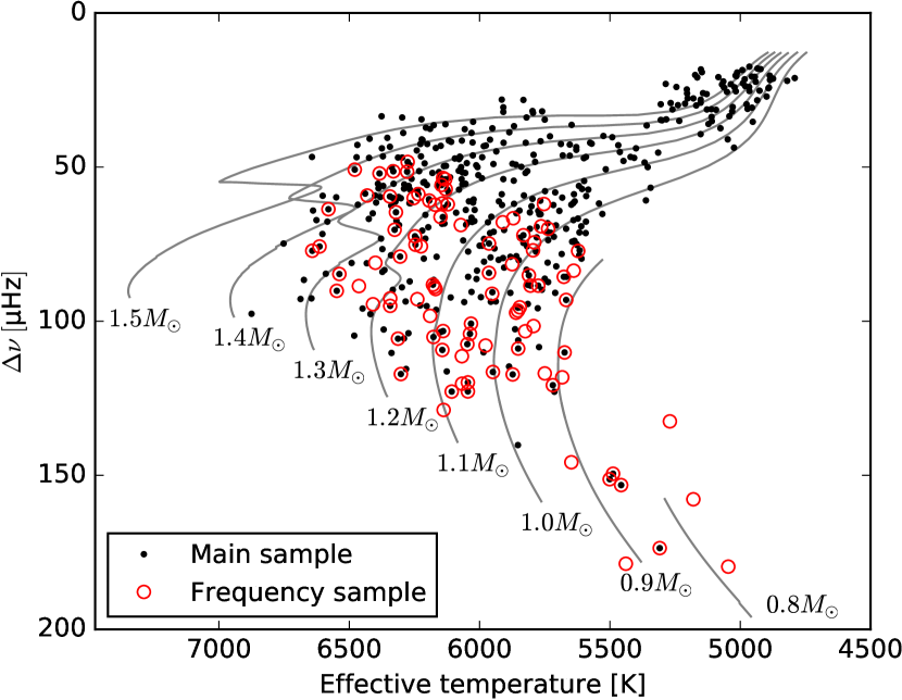
Figure 1: Observed $\Delta\nu$ and spectroscopic temperature of the main and frequency samples. The lines show evolutionary tracks computed with GARSTEC for models with solar metallicity and masses as labelled.

Both samples are shown in Figure 1 in the space of observed $\Delta\nu$ and spectroscopic $T_{\mathrm{eff}}$ along with evolutionary tracks computed using the Garching Stellar Evoluion Code (GARSTEC; Weiss & Schlattl 2008). With the visual aid of the evolutionary tracks, it is clear that the stars in the frequency sample are generally less evolved than the stars in the main sample. This is mainly due to the fact that the stars of the frequency sample have been selected to be on the main sequence in order to avoid the complications of modelling mixed dipole modes which show up in the oscillation spectra of more evolved stars.

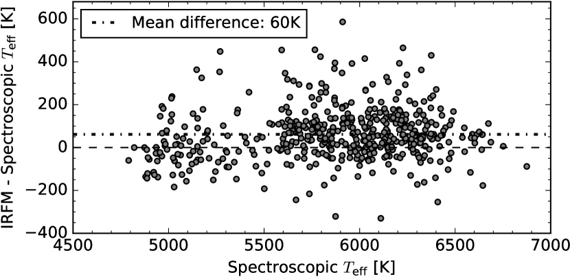
Figure 2: Difference between the two sets of temperatures (IRFM and spectroscopic) which have been collected for the full sample. On average, the IRFM temperatures are higher and the dot-dashed line shows the mean difference which is 60 K.

Finally, a second effective temperature has been derived for the full sample using the Infrared Flux Method (IRFM) as implemented by Casagrande et al. (2006); Casagrande et al. (2010) (the procedure is described in subsection 3.2). In Figure 2 the differences between the IRFM and spectroscopic temperatures are shown. The scatter is quite large (about 150 K) and, on average, the IRFM temperatures are higher than the spectroscopic ones by about 60 K; however, this mean offset does not apply to the entire range of temperatures of the sample. If only the stars with temperatures below 5500 K are considered, which are mostly subgiants (see Figure 1), the mean offset is instead around just 10 K (but still with a large scatter). For stars with temperatures above 5500 K, the mean offset agrees with the overall mean of 60 K which is also the case for both the main and frequency samples when considered individually.

3 Methods

3.1 Radii

The scaling relations for the average asteroseismic parameters $\Delta\nu$ and $\nu_{\mathrm{max}}$ are given by (Ulrich, 1986; Brown et al., 1991)

$$\frac{\Delta\nu}{\Delta\nu_{\sun}} \simeq\left(\frac{M}{M_{\sun}}\right)^{1/2}\left(\frac{R}{R_{\sun}}\right)^{-3/2}\;,$$ (1)

$$\frac{\nu_{\mathrm{max}}}{\nu_{\mathrm{max},\sun}} \simeq\left(\frac{M}{M_{\sun}}\right)\left(\frac{R}{R_{\sun}}\right)^{-2}\left(\frac{T_{\mathrm{eff}}}{T_{\mathrm{eff},\sun}}\right)^{-1/2}\;,$$ (2)

which can be rearranged to give the scaling relations for the radius and mass

$$\frac{R}{R_{\sun}} \simeq\left(\frac{\nu_{\mathrm{max}}}{\nu_{\mathrm{max},\sun}}\right)\left(\frac{\Delta\nu}{\Delta\nu_{\sun}}\right)^{-2}\left(\frac{T_{\mathrm{eff}}}{T_{\mathrm{eff},\sun}}\right)^{1/2}\;,$$ (3)

$$\frac{M}{M_{\sun}} \simeq\left(\frac{\nu_{\mathrm{max}}}{\nu_{\mathrm{max},\sun}}\right)^{3}\left(\frac{\Delta\nu}{\Delta\nu_{\sun}}\right)^{-4}\left(\frac{T_{\mathrm{eff}}}{T_{\mathrm{eff},\sun}}\right)^{3/2}\;.$$ (4)

The scaling relations have been applied to both stellar samples using the two different effective temperature scales resulting in two sets of stellar parameters. The solar values are taken to be $\nu_{\mathrm{max,\sun}}=3090~{}\mathrm{\upmu Hz}$, $\Delta\nu_{\sun}=135.1~{}\mathrm{\upmu Hz}$ (Huber et al., 2011), and $T_{\mathrm{eff,\sun}}=5777~{}\mathrm{K}$.

In order to take advantage of the individual frequencies, the stars of the frequency sample have been fitted to a grid of GARSTEC stellar models with theoretical oscillation frequencies computed using the Aarhus adiabatic oscillation package (ADIPLS, Christensen-Dalsgaard 2008). The stellar models have been computed with the OPAL equation of state (Rogers & Nayfonov, 2002), OPAL opacitites (Iglesias & Rogers, 1996) with low-temperature opacities by Ferguson et al. (2005), the NACRE compilation of nuclear reaction rates (Angulo et al., 1999), and the solar mixture of Grevesse & Sauval (1998). Convection is implemented in the mixing length formalism and we use a solar-calibrated mixing length parameter of $\alpha_{\mathrm{mlt}}=1.7917$. The solar-calibrated initial composition of $Y_{i}=0.2705$ and $Z_{i}=0.0189$ has been combined with the Big Bang nucleosynthesis values of $Y_{0}=0.2482$ and $Z_{0}=0$ (Steigman, 2010) to get a helium enrichment law of $\Delta Y/\Delta Z=1.179$. This has been used in all models to define the initial helium abundance for a given initial metallicity $[\mathrm{Fe}/\mathrm{H}]$.

Two grids of stellar models have been computed: one including microscopic diffusion and the other including convective overshoot using the diffusion formalism implemented in GARSTEC with an efficiency parameter of $f=0.016$ (see Weiss & Schlattl 2008, section 3.1.5). The diffusion grid spans masses of 0.70–1.30 $M_{\sun}$ and the overshoot grid spans masses of 1.00–1.80 $M_{\sun}$, both in steps of 0.01 $M_{\sun}$. Initial metallicities from -0.65 to +0.55 dex in steps of 0.05 dex are included in the overshoot grid and for the diffusion grid the initial values have been increased slightly, thus covering the range -0.60 to +0.65 dex, in order to account for the decrease in surface metallicity with evolution. Both grids cover $\Delta\nu$, as calculated from Equation 1, in the range 13–180 $\upmu$Hz, which spans the entire observed range including some room for inaccuracies in the scaling relations. All stars were fitted to both model grids and for the ones that returned masses in the range of overlap (1.00–1.30 $M_{\sun}$), we choose, by visual inspection, the fit for which the probability distribution of the mass is not cut off by the edge of the grid. If none of the two fits hit the edge, we compare the observed and modelled oscillation frequencies, effectively choosing the grid for which the best fitting model has the highest likelihood. Small individual diffusion grids were computed for the three stars with metallicities lower than -0.60 dex.

For all fits to the grids, metallicities and temperatures are included in addition to the asteroseismic observables. Like for the scaling relations, this gives two sets of stellar parameters corresponding to the use of the two different temperature scales. Theoretical stellar oscillations are affected by systematic errors caused by improper modelling of the outer stellar layers in current stellar models. Therefore, when fitting the observed oscillation frequencies to the model grids, we have to correct the model frequencies or use certain ratios of frequency differences which have been shown to be insensitive to the surface layers (Roxburgh & Vorontsov, 2003). Using the Bayesian Stellar Algorithm (BASTA, see Silva Aguirre et al. 2015) we have fitted the stars to both frequency ratios and to individual frequencies after applying the correction introduced by Ball & Gizon (2014) for the surface effect. These two methods give very similar results with a mean radius difference of less than 0.1% and a scatter of 0.7%. Thus, the choice between fitting to frequency ratios or corrected individual frequencies has no significant impact on the final results, and the stellar parameters based on fits to frequency ratios will be used in the following.

The grid-based method has also been applied to the stars of the main sample by fitting the observed $\Delta\nu$ to the mean frequency separation of the radial model frequencies, $\Delta\nu_{\mathrm{fit}}$, calculated as described by White et al. (2011). This quantity is also sensitive to the surface effect; therefore, we have scaled the grid values by the ratio of the observed solar frequency separation, $\Delta\nu_{\sun}=135.1~{}\mathrm{\upmu Hz}$, and that of the solar model calibration, $\Delta\nu_{\mathrm{fit,sunmod}}=136.1~{}\mathrm{\upmu Hz}$. By applying this scaling, the surface effect is assumed to increase the value of $\Delta\nu$ by a constant fraction of 1.007 for all stars. Note that $\nu_{\mathrm{max}}$ has not been included in these model fits in order to get a set of stellar parameters independent of the scaling relations. It turns out, however, that it makes no difference whether it is included or not because the typical relative uncertainty on $\nu_{\mathrm{max}}$ of 4.3% for the stars of the main sample is too large to impose any significant constraint on the models.

3.2 Distances

In order to calculate asteroseismic distances, and thereby parallaxes, we have used the distance modulus based on the magnitudes in the $griz$ and $JHK_{s}$ photometric filters, and the implementation is divided into two steps. The first step of the calculation is to determine the reddening in a way to make it consistent with the final distance. This is done by an iterative procedure starting with the value of $E(B-V)$ from the KIC. This value of the color excess is used as input for the bolometric correction software by Casagrande & VandenBerg (2014) (as implemented in BASTA) together with the observed surface properties $T_{\mathrm{eff}}$ (spectroscopic or IRFM depending on which was used to determine the stellar properties), $[\mathrm{Fe}/\mathrm{H}]$, and the surface gravity $\log g$ obtained from the asteroseismic analysis. The output is the extinction-corrected bolometric corrections for each of the photometric filters. With each observed magnitude and theoretical bolometric correction, the distance is calculated using the luminosity from asteroseismology and the absolute bolometric magnitude of the Sun $M_{\mathrm{bol},\sun}=4.75$. The final distance is determined by taking the median of the values from the different filters. With this distance, the color excess is updated using the 3D dust map by Green et al. (2015) and the process is iterated twice, at which point the color excess has converged to within 0.01 mag.

The second step of the distance calculation is to determine the distances and uncertainties using the final color excess obtained in step one. For this purpose, we apply Monte Carlo sampling using the uncertainties on all input parameters assuming Gaussian error distributions. The values and uncertainties for $T_{\mathrm{eff}}$, $[\mathrm{Fe}/\mathrm{H}]$, and the $JHK_{s}$ magnitudes are taken from the input catalogues. No individual uncertainties are given for the $griz$ magnitudes in the KIC so they are simply all set to 0.02 mag which is the level of precision found by Brown et al. (2011) based on repeatability of the photometry. Uncertainties on the luminosity and surface gravity are taken from the results of the asteroseismic analysis.

We have also combined the asteroseismic scaling relations with the IRFM in the way described by Silva Aguirre et al. (2012) to derive a set of self-consistent temperatures (the ones introduced in section 2), radii, angular diameters, and hence distances. For this procedure the 3D dust map by Green et al. (2015) has also been used iteratively. We applied the IRFM twice using different input photometry in the visible. One set was obtained using the $B_{T}$ and $V_{T}$ bands of the Tycho-2 catalogue (Høg et al., 2000) and the other set made use of the $griz$ bands from the KIC. In both cases, the 2MASS $JHK_{s}$ bands were used in the infrared. This was done since either set of visible photometry may be problematic in some cases. For example, for the two brightest stars of this study, 16 Cygni A & B, we find the parallaxes to be underestimated when using the KIC photometry (compared to the Gaia observations), but not when using Tycho-2 photometry, which indicates problems with the photometry in the $griz$ filters for these stars. On the other hand, the quality of the Tycho-2 photometry is worse for the faintest stars. An initial comparison between the two sets of temperatures showed large discrepancies with differences above 200 K for about 15% of the stars. Therefore, we decided to use a third set of temperatures for comparison in order to choose, on a star-by-star basis, which of the two temperatures from the IRFM to use. The third set was calculated from 2MASS photometry only, which is usually good over a wide range of magnitudes, using a color-temperature calibration linking $J-K_{s}$ to $T_{\mathrm{eff}}$. For each star, the final temperature was chosen to be the IRFM temperature which was closest to the one from the 2MASS color calibration. With this criterion, the KIC ($griz$) set of temperatures and angular diameters was used for 53% of the stars and the Tycho-2 ($B_{T}V_{T}$) set was used for the remaining 47%. We could of course have used the 2MASS temperatures directly; however, this would defeat the purpose of using the IRFM which is to obtain a set of self-consistent temperatures, radii, and distances.

In principle, the IRFM parameters should be derived anew when using the individual frequencies, instead of the scaling relations, to derive stellar parameters. However, in practice, the radii which are used to get the distances do not change enough for the changes in reddening to be significant. A test showed that for the majority of the frequency sample the difference in $E(B-V)$ is at the level of 0.001 mag. This level of agreement translates to a difference in $T_{\mathrm{eff}}$ of just a few kelvin which is well below the statistical uncertainties.

4 Results

4.1 Parallax comparisons for the frequency sample

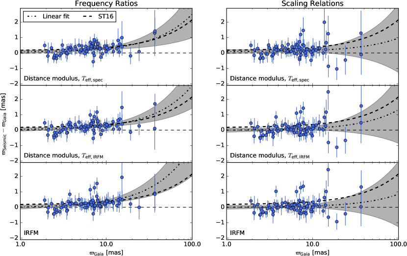
Figure 3: Absolute differences between seismic and Gaia parallaxes as a function of Gaia parallax for the frequency sample. The dot-dashed lines are linear fits to the data which are weighted according to the uncertainties and the thick dashed line is the linear relation found by ST16 based on radii of eclipsing binaries (the lines curve due to the logarithmic x-axis). Grey shaded areas indicate the 1$\sigma$-region of the linear fits. The left- and right-hand columns show results based on frequency ratio fits and the scaling relations, respectively. The rows show different methods for calculating seismic distances (and hence parallaxes) as labelled.

Based on the seismic distances, $d_{\mathrm{seis}}$, we simply calculate the seismic parallaxes as $\varpi_{\mathrm{seis}}=1/d_{\mathrm{seis}}$. In Figure 3 the absolute differences between the seismic and Gaia parallaxes are plotted as a function of the Gaia parallaxes for the frequency sample. The columns show the two different methods used to derive stellar properties, and the rows show the different methods for calculating distances. A number of outliers were identified in the original study of the LEGACY sample, and all of the stars they found to be problematic have been excluded from this comparison. They quoted several sources to argue that the offsets are mainly due to contaminated photometry. For example, some of the stars are binaries and their flux measurements include the contributions from both components (see the discussion in Silva Aguirre et al. 2017, section 5.3).

If we first consider the results based on fits to frequency ratios (left-hand column), there is good agreement overall and individual differences are generally within the statistical uncertainties. However, there is also a trend towards seismic parallaxes being too large on average. For the results based on spectroscopic temperatures, the weighted mean difference is $\Delta\varpi=(0.21\pm 0.04)~{}\mathrm{mas}$, and the offset also seems to be distance dependent as indicated by the linear fit to the data which is weighted according to the plotted uncertainties. Based on this fit, the difference as a function of parallax is approximately given by

$$\Delta\varpi=(0.03\varpi+0.03)~{}\mathrm{mas}\,.$$ (5)

This is similar to what was found by ST16 based on radii of eclipsing binaries (dashed lines in the figure), but their linear relation predicts a slightly larger offset at low parallaxes (with an intersection at 0.16 mas) which is just outside the $1\sigma$-region of what is found here. For parallaxes ${\gtrsim}10~{}\mathrm{mas}$ the two linear relations agree. A distance dependent absolute offset means that the relative offset is constant across all distances. The weighted mean parallax ratio is $1.029\pm 0.006$, meaning that the seismic parallaxes are overestimated by about 3% assuming that the Gaia parallaxes are unbiased.

An overestimation of the seismic parallaxes is exactly what we would expect to get if the temperatures are underestimated. Higher temperatures will lead to higher luminosities which increase the derived distances and lowers the parallaxes. Comparing the stellar parameters obtained with the two sets of temperatures, the increase of about 60 K on average leads to best-fitting models which are ${\sim}2\%$ more luminous. The mean change in radius, however, is below 0.1% which means that the entire increase in luminosity is due to the best-fitting models being hotter. Comparing the upper two panels, which differ only in the adopted temperatures, we see that the parallaxes are still too high on average. Surprisingly, with the IRFM temperatures, the weighted mean ratio has not decreased. In fact, it has increased slightly (but not significantly) to $1.031\pm 0.006$ for the results using the distance modulus. As argued above, higher luminosities should lead to lower parallaxes and better overall agreement with the Gaia data. Based on the proportionality from the distance modulus $\varpi\propto(L/L_{\odot})^{-1/2}$, the parallaxes are expected to decrease by about $1\%$ due to the luminosity increase of $2\%$. If we instead compare the median ratios, the results are $1.041$ and $1.033$ with the spectroscopic and IRFM temperatures, respectively. This is more in line with our expectations and indicates that the parallaxes have decreased overall, but the stars with high weights (i.e. low statistical uncertainties) have retained their seismic parallax value. In any case, there is a systematic offset at the level of $3\%$ regardless of the adopted temperature scale. A comparison between the two lower panels shows that the two different methods used to calculate distances agree very well. When comparing the two sets of seismic parallaxes directly, they are found to agree within 0.2% on average even though different photometry was used in the visible for two-thirds of the stars (which is the fraction of the frequency sample for which the Tycho-2 photometry was used to derive the IRFM temperatures).

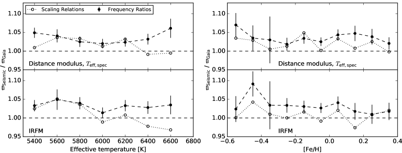
Figure 4: Ratios of seismic and Gaia parallaxes as a function of effective temperature (left) and metallicity (right) for the frequency sample. The data are shown as weighted mean bins with equal separation. Errorbars on the binned data are shown for the results based on frequency ratios to give a sense of the uncertainty at a given value on the x-axis. The most metal-poor star of the sample ($[\mathrm{Fe}/\mathrm{H}]=-0.92$) has been excluded in the right-hand panel.

Turning to the results based on the scaling relations (right-hand column of Figure 3), the mean parallax offset has decreased compared to the results based on ratio fits. For the spectroscopic temperatures, the weighted mean difference is $\Delta\varpi=(0.14\pm 0.05)~{}\mathrm{mas}$ which still implies that the seismic parallaxes are too high. In this case, however, the temperature scale does make a difference since it enters explicitly into the scaling relations, and with IRFM temperatures and angular diameters the offset decreases to just $\Delta\varpi=(0.05\pm 0.05)~{}\mathrm{mas}$, consistent with no offset. Note also that for both temperature scales the slope of the linear fit is not significantly different from zero, and for the IRFM temperatures the offset is clearly not compatible with the results of ST16 at low parallaxes. This stands in contrast to the results based on ratio fits where the slope is significant regardless of the adopted temperatures.

These results corroborate the findings of Huber et al. (2017), namely that the hotter IRFM temperatures lead to better agreement between seismic (from scaling relations) and Gaia parallaxes, and that the offset identified by ST16 may be overestimated for low parallaxes. However, the offset found by Silva Aguirre et al. (2017) for the LEGACY sample has not been reduced by the inclusion of the Kages stars or by the change in temperature. This leads to an interesting tension between the scaling relations giving good agreement with the Gaia parallaxes and the fits to frequency ratios showing a constant offset of a few percent.

The differences between the results from the scaling relations and the ratio fits, and the impact of the temperature scale, become clearer when the results are plotted together as a function of temperature as shown in the left-hand panel of Figure 4. To avoid clutter, only the weighted mean bins are shown, and the error bars, which are of similar magnitude for all data points at a given temperature, are only shown for the ratio fits. At the lowest temperatures, the scaling relations generally agree well with the ratio fits for both temperature scales. However, at higher temperatures the scaling relations deviate from the ratio fits and result in lower parallaxes. So the main reason that the parallaxes from the scaling relations show overall better agreement with Gaia seems to be a deviation from the ratio fits at high temperatures. There are also differences between the two applications of the scaling relation (upper and lower panel) due to the different temperatures. At high temperatures ($T_{\mathrm{eff}}>5800~{}\mathrm{K}$) the IRFM results give lower seismic parallaxes than the spectroscopic results and vice versa at the lower temperatures. This is what makes the IRFM results compatible with the Gaia data (on average), and it is simply a reflection of differences in the temperature scales.

The right-hand panel of Figure 4 shows the parallax comparison as a function of metallicity where no significant trends are found. Here the difference between the scaling relations and the ratio fits show up as a constant offset which does not depend on the metallicity.

Since the scaling relations are anchored to the solar values, they are naturally thought to be most accurate for stars like the Sun. Therefore, it is interesting that the parallaxes based on the scaling relations agree so well with the ones from frequency ratios at near-solar temperatures and only deviate at the highest temperatures considered in this study. This indicates that either the asteroseismic radii are underestimated at temperatures around that of the Sun, and the scaling relations become more accurate at higher temperatures, or, which seems more likely, that there is a bias in either the Gaia parallaxes or the calculation of seismic parallaxes, and that the scaling relations overestimate the radii at high temperatures. If the deviation between the two methods at high temperatures is indeed due to inaccuracies in the scaling relations, we are still left with the problem of explaining a 3% offset in seismic parallaxes based on fits to frequency ratios.

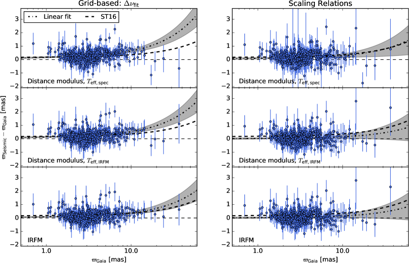
Figure 5: Same as Figure 3 but for the main sample with the grid-based results based on $\Delta\nu_{\mathrm{fit}}$ instead of frequency ratios.

The Gaia parallaxes are known to suffer from position and colour dependent systematic errors at a level of $\pm$0.3 mas (Lindegren et al., 2016). This may explain part of the observed offset; however, it seems unlikely to explain a constant fractional offset such as the one found here. A fractional offset may instead be introduced in the conversion between seismic radii and parallaxes. Huber et al. (2017) tested the use of different ways to determine bolometric corrections and found that it can lead to systematic errors of around 1% in parallax due to the use of different model atmospheres and methods for extracting the synthetic fluxes. It is also possible that the extinction values of the 3D map are biased. In order to decrease the seismic parallaxes and bring them into agreement with the Gaia values, the degree of extinction has to be decreased. However, the stars considered here are not very distant ($d<1~{}\mathrm{kpc}$), and the median extinction in the visible is only about 0.03 mag based on the extinction map. For comparison, a difference of about 0.06 magnitudes is necessary in order to explain a relative difference of 3% in parallax.

It is also worth discussing what could lead to underestimated seismic radii from the ratio fits, if that is in fact the cause of the offset. The most obvious sources of bias in the stellar parameters are the model physics that have been fixed based on e.g. a solar calibration. For example, the mixing length parameter $\alpha_{\text{mlt}}$ is fixed at the solar-calibrated value of $1.791$ in all models. However, 3D simulations of convection have shown that the convective efficiency varies with temperature and surface gravity (e.g. Trampedach et al. 2014). Additionally, there is a known degeneracy between the initial helium abundance and the stellar mass (Silva Aguirre et al., 2015) and, for the grids used in this study, the initial helium abundance is fixed for any given metallicity by the enrichment law $\Delta Y/\Delta Z=1.179$. Finally, the overshoot efficiency directly influences the obtained masses for stars with convective cores.

Now the question is whether the effects of fixing the model physics are large enough to explain the observed parallax offset. In the original study of the LEGACY sample (Silva Aguirre et al., 2017), a number of different stellar model grids and fitting algorithms were applied. Most notably, a number of the algorithms left the values of $\alpha_{\text{mlt}}$ and the initial helium abundance as free parameters to be optimized during the fit. Even with this variety of methods, the overall agreement between the radii was good (with typical mean offsets between the methods below 1%) and the parallax offset compared to the Gaia values was seen with every method. Therefore, model physics are only able to explain part of the offset unless more fundamental features of the models like the opacities or the equation of state need adjustments.

All things considered, it is not possible to point to any one part of the analysis as the sole source of the observed offset. It may be caused by any combination of the different factors that have been discussed, including of course the seismic radii. What can be said, however, is that there are no indications of deviations from the scaling relation for the radius by more than 5% based on these parallax comparisons.

4.2 Parallax comparisons for the main sample

In Figure 5 the absolute differences between the seismic and Gaia parallaxes are shown for the main sample. One feature which must be mentioned is the tendency for the offset to be systematically positive at the lowest parallaxes. This happens because the Gaia parallaxes are less precise than the seismic ones, and therefore scatter to lower values causing a positive offset. Similarly, when they scatter to higher values the offset is negative, and the combined effect is a diagonal edge at low parallaxes.

Like we saw for the ratio fits of the frequency sample, the grid-based method results in absolute offsets which increase with parallax. Due to the diagonal edge at low parallaxes, only stars with $\varpi_{\mathrm{Gaia}}>2.5~{}\mathrm{mas}$ have been included in the linear fits. With spectroscopic temperatures the weighted mean difference is $\Delta\varpi=(0.28\pm 0.02)~{}\mathrm{mas}$, and the linear fit is given approximately by

$$\Delta\varpi=0.06\varpi+0.07\,.$$ (6)

This slope is double the value found for the ratio fits and by ST16. The weighted mean relative offset has also doubled to $(6.0\pm 0.4)\%$.

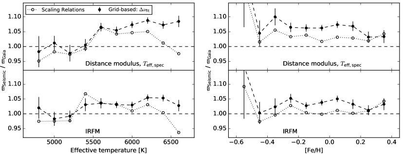
Figure 6: Same as Figure 4 but for the main sample with the grid-based results based on $\Delta\nu_{\mathrm{fit}}$ instead of frequency ratios. The two most metal-poor stars of the sample ($[\mathrm{Fe}/\mathrm{H}]=-0.92,-1.75$) have been excluded in the right-hand panel.

The temperature carries more weight in the fits to $\Delta\nu_{\mathrm{fit}}$ of the main sample than it did for the fits to frequency ratios, and the change to IRFM temperatures has a larger impact. Changing from spectroscopic temperatures and the distance modulus to IRFM temperatures and angular diameters, the weighted mean parallax offset is reduced to $(3.3\pm 0.4)\%$, bringing it much closer to the results of the frequency sample and ST16. The combination of IRFM temperatures and the distance modulus gives an offset of $(4.9\pm 0.4)\%$ which falls right in between the two extremes. Thus, the mean offset gradually decreases when going from the upper to the lower panels of Figure 5.

Like for the frequency sample, the scaling relations lower both the overall offset between the parallaxes and the slopes of the linear fits. For the spectroscopic and IRFM temperatures, the weighted mean differences are $\Delta\varpi=(0.16\pm 0.02)~{}\mathrm{mas}$ and $(0.07\pm 0.02)~{}\mathrm{mas}$, respectively, in agreement with the offsets found with the scaling relations for the frequency sample, but with lower uncertainties owing to the larger sample size. The slope is only just significant within one standard deviation for the spectroscopic temperatures, but for the IRFM temperatures it is insignificant. It is also seen once again that the relation from ST16 overestimates the offset at low parallaxes compared to the results found here with both temperature scales.

In Figure 6 the weighted mean bins from the scaling relations and the fits to $\Delta\nu_{\mathrm{fit}}$ are compared directly for the two sets of temperatures. The scaling relations follow the fits to $\Delta\nu_{\mathrm{fit}}$ at low temperatures where the seismic parallaxes show the best agreement with Gaia. For higher temperatures, i.e. $T_{\mathrm{eff}}\gtrsim 6000~{}\mathrm{K}$ the two methods begin to increasingly deviate. Note how similar the trend is to the one for the frequency sample (Figure 4) if the temperatures below 5500 K are ignored. In this region, both samples agree that the seismic parallaxes based on the scaling relations change with temperature while the methods independent of the scaling relations show a nearly constant offset. Also like for the frequency sample, there are no significant trends with metallicity.

4.3 Corrections to the scaling relations

If we assume that the parallax differences seen in Figure 4 and Figure 6 are solely due to errors in the seismic radii, the scaling relation for the radius needs a correction, depending on the temperature, with a maximum value of about 5%. For example, using the results from the IRFM, the radii are, on average, underestimated at the solar temperature and overestimated at the highest temperatures in the sample. The best agreement between the parallaxes is found for the subgiants in the main sample which suggests that little or no correction is needed to the scaling relation for these stars.

The fact that both the parallaxes from the scaling relations and from frequency modelling show an offset at the solar temperature (where the scaling relations are thought to be accurate for dwarf stars) leads us to consider the alternate assumption that there is a bias in either the Gaia parallaxes or in the quantities involved in transforming the seismic radii into distances (i.e. bolometric corrections and extinctions). The parallax comparisons show that the radii of the scaling relations deviate from those of the grid-based analyses, which are independent of the scaling relations, at high effective temperatures. Even though the scaling relations give parallaxes which agree better with the Gaia data on average, it seems most likely that the trend with temperature reflects a problem with the scaling relations. In the following, we attempt to quantify this temperature trend and correct the scaling relations for it. We will use the stellar parameters obtained from the ratio fits (with IRFM temperatures) as reference values. Despite the constant parallax offset of 3%, these radii and masses are very precise and they are internally consistent within the adopted stellar models. Thus we consider them to be the best available substitute for the true values. However, it should be kept in mind that the validity of the corrections we obtain for the scaling relations depend on the assumption that the parallax offset of 3%, between parallaxes from Gaia and from fitting to frequency ratios, is not due to systematic errors in the seismic radii. We also assume that the temperature trend is not due to a potential temperature dependent bias in the IRFM temperatures.

We take the stellar radii, masses, and temperatures from the best-fitting models and calculate the model values $\Delta\nu_{\mathrm{scaling}}$ and $\nu_{\mathrm{max,scaling}}$ based on the scaling relations (Equation 1 and Equation 2). It is interesting whether or not the deviations between $\Delta\nu_{\mathrm{scaling}}$, $\nu_{\mathrm{max,scaling}}$ and the observed values depend on the physical parameters of the stars. If they do, it is possible to define corrections to the scaling relations which will bring the radii and masses calculated from them into line with the ones found from the ratio fits. Since this analysis does not depend on the Gaia parallaxes we have included the LEGACY and Kages stars which were not a part of the GDR1, increasing the sample size from 86 to 95 stars.

As we saw in the parallax comparisons, the difference between the radii obtained from the ratio fits and those given by the scaling relations varies as a function of temperature. This suggests that corrections to the scaling relations for $\Delta\nu$ and $\nu_{\mathrm{max}}$ should at least depend on temperature. For $\Delta\nu$ this is no surprise since previous studies (e.g. White et al. 2011) already showed that the difference between $\Delta\nu_{\mathrm{fit}}$ and $\Delta\nu$ from the scaling relation is mainly a function of temperature. However, using the masses and radii of the ratio fits it will be possible to investigate potential corrections to the scaling relation for $\nu_{\mathrm{max}}$ as well. Defining the two functions $f_{\Delta\nu}(T_{\mathrm{eff}})$ and $f_{\nu_{\mathrm{max}}}(T_{\mathrm{eff}})$ as the temperature dependent corrections to the scaling relations for $\Delta\nu$ and $\nu_{\mathrm{max}}$, respectively, the corrected versions of Equations 1 and 2 are given by

$$\frac{\Delta\nu}{\Delta\nu_{\sun}} \simeq\left(\frac{M}{M_{\sun}}\right)^{1/2}\left(\frac{R}{R_{\sun}}\right)^{-3/2}f_{\Delta\nu}(T_{\mathrm{eff}})\;,$$ (7)

$$\frac{\nu_{\mathrm{max}}}{\nu_{\mathrm{max},\sun}} \simeq\left(\frac{M}{M_{\sun}}\right)\left(\frac{R}{R_{\sun}}\right)^{-2}\left(\frac{T_{\mathrm{eff}}}{T_{\mathrm{eff},\sun}}\right)^{-1/2}f_{\nu_{\mathrm{max}}}(T_{\mathrm{eff}})\;,$$ (8)

from which the corrected scaling relations for the mass and radius follow

$$\frac{M}{M_{\sun}} \simeq\left(\frac{\nu_{\mathrm{max}}}{\nu_{\mathrm{max},\sun}}\right)^{3}\left(\frac{\Delta\nu}{\Delta\nu_{\sun}}\right)^{-4}\left(\frac{T_{\mathrm{eff}}}{T_{\mathrm{eff},\sun}}\right)^{3/2}f_{\nu_{\mathrm{max}}}^{-3}(T_{\mathrm{eff}})f_{\Delta\nu}^{4}(T_{\mathrm{eff}})\;,$$ (9)

$$\frac{R}{R_{\sun}} \simeq\left(\frac{\nu_{\mathrm{max}}}{\nu_{\mathrm{max},\sun}}\right)\left(\frac{\Delta\nu}{\Delta\nu_{\sun}}\right)^{-2}\left(\frac{T_{\mathrm{eff}}}{T_{\mathrm{eff},\sun}}\right)^{1/2}f_{\nu_{\mathrm{max}}}^{-1}(T_{\mathrm{eff}})f_{\Delta\nu}^{2}(T_{\mathrm{eff}})\;.$$ (10)

The combinations of correction factors in these equations can be defined as correction factors for the mass $f_{M}=f_{\nu_{\mathrm{max}}}^{-3}f_{\Delta\nu}^{4}$, and the radius $f_{R}=f_{\nu_{\mathrm{max}}}^{-1}f_{\Delta\nu}^{2}$. Corrections that apply to the frequency sample can be obtained by comparing the observed and modelled asteroseismic parameters as a function of temperature. Only the stars with effective temperatures higher than 5500 K will be used in this analysis due to the poor sample size at lower temperatures.

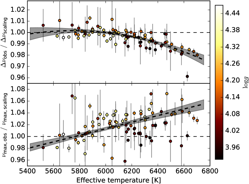
Figure 7: Ratio of observed and scaling relation $\Delta\nu$ (upper panel) and $\nu_{\mathrm{max}}$ (lower panel) as a function of IRFM effective temperature with error bars indicating the uncertainties on the observed values. The scaling relation values are taken from the best-fitting models of the ratio fits and depend on the models’ masses, radii, and temperatures. The data are color coded according to surface gravity and the dashed lines are the best-fitting relations discussed in the text. The shaded areas indicate the bootstrapped uncertainties of the fits.

In Figure 7, the ratios of observed and scaling relation $\Delta\nu$ and $\nu_{\mathrm{max}}$ are shown as a function of observed effective temperature and color coded by surface gravity. The error bars only include the statistical uncertainty on the observed values. Inspired by the functional form of the correction found by White et al. (2011) a second order polynomial has been fitted to the data for $\Delta\nu$. The fit follows the data nicely, and the residual scatter is at a level of ${\sim}1\%$. For this limited range of surface gravities, there is no strong indication that the offset depends on the value of $\log g$. Based on the fit, the correction factor for $\Delta\nu$ is given by

$$f_{\Delta\nu}(T_{\mathrm{eff}})=-2.52\left(\frac{T_{\mathrm{eff}}}{10^{4}\mathrm{K}}\right)^{2}+2.90\left(\frac{T_{\mathrm{eff}}}{10^{4}\mathrm{K}}\right)+0.17\;,$$ (11)

which applies in the range of temperatures and surface gravities covered in the figure. This expression gives a small correction of $f_{\Delta\nu}(T_{\mathrm{eff},\sun})=1.002$ at the solar temperature which is not ideal considering that the scaling relations are anchored to the solar values. One could add a constraint on the fit to make it hit unity at the solar temperature, but since the deviation is within the uncertainty (shaded area in the figure), we have chosen not to do so.

For $\nu_{\mathrm{max}}$ the uncertainties are larger and the data points are much more scattered at any given temperature. Although the correlation with temperature is less clear, the offset does seem to increase slightly with increasing temperature. The linear fit shown in the figure implies a correction factor of

$$f_{\nu_{\mathrm{max}}}(T_{\mathrm{eff}})=0.397\left(\frac{T_{\mathrm{eff}}}{10^{4}\mathrm{K}}\right)+0.771\;.$$ (12)

Like for the $\Delta\nu$ correction, the fit hits unity at the solar temperature within the uncertainty and has not been constrained. The large scatter around this relation is partly due to the uncertainties on the observed values, but it may also suggest that the offset depends on more than just temperature. Most of the stars with low surface gravities seem to fall below the linear fit which indicates that the correlation can be improved by including a $\log g$ term. A dependence on surface gravity is reasonable considering it is the other factor, besides the temperature, which enters into the $\nu_{\mathrm{max}}$ scaling relation. Additionally, a dependence on metallicity is not unthinkable considering that Viani et al. (2017) recently pointed out that the approximation usually adopted for the acoustic cut-off frequency $\nu_{\mathrm{ac}}$ (and therefore also $\nu_{\mathrm{max}}$) lacks a factor related to the mean molecular weight. However, no significant correlations with these parameters have been found. A direct comparison between $\nu_{\mathrm{max,obs}}/\nu_{\mathrm{max,scaling}}$ and the metallicity, showing no significant correlation, is given in Figure 8. Similarly, no significant correlation is found with $\log g$. Thus, the dependence of the correction on surface gravity and metallicity is not very strong, and the simple relation in Equation 12 has been adopted as the correction to $\nu_{\mathrm{max}}$ in the following.

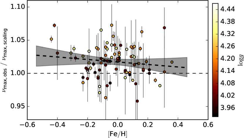
Figure 8: Ratio of observed and scaling relation $\nu_{\mathrm{max}}$ as a function of spectroscopic metallicity with errorbars indicating the uncertainty on the observed values. The scaling relation values are taken from the best-fitting models of the ratio-fits and depend on the models’ masses, radii, and temperatures (using the IRFM set). The data are color coded according to surface gravity and the dashed line is the best linear fit. The shaded area indicates the bootstrapped uncertainty of the fit.

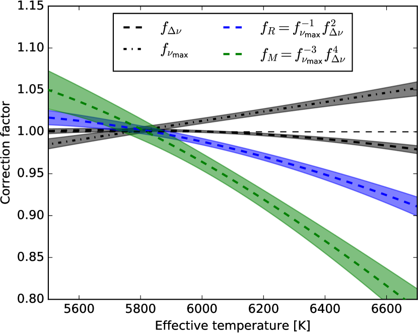
Figure 9: Corrections to $\Delta\nu$ (black dashed), $\nu_{\mathrm{max}}$ (black dot-dashed), and the resulting corrections to the scaling relations for the radius (blue) and mass (green).

Figure 9 shows the corrections obtained for $\Delta\nu$ and $\nu_{\mathrm{max}}$ as well as the corrections they imply for the scaling relations giving the mass and radius. The correction to $\nu_{\mathrm{max}}$ is greater than the correction to $\Delta\nu$ at all temperatures; however, due to the greater exponent on $\Delta\nu$ in the scaling relations, the two corrections have an almost equal impact on the stellar radius and mass at the highest temperatures. These corrections imply that the scaling relations overestimate the radii and masses of main-sequence stars by $(8\pm 1.5)\%$ and $(22\pm 4)\%$, respectively, at a temperature of 6600 K. However, they also show that for main-sequence stars with temperatures below 6400 K (which is 85% of the stars in this study) radii and masses from the scaling relations are accurate to within 5% and 13%, respectively. Due mostly to the large scatter around $f_{\nu_{\mathrm{max}}}$, these numbers represent averages for the frequency sample and do not apply to each of the stars individually.

Coelho et al. (2015) performed a test of the $\nu_{\mathrm{max}}$ scaling relation using the same method applied here, but to about 400 of the Kepler dwarfs with fits to $\Delta\nu_{\mathrm{fit}}$ instead of frequency ratios. They only found a constant offset from the scaling relation of a few percent and no significant trend with temperature. Even though the results presented here are based on frequency ratios which give more precise (and likely accurate) stellar parameters than $\Delta\nu_{\mathrm{fit}}$, the sample size is also considerably smaller, and it is not unthinkable that the trend disappears with more observations. In fact, if all data points below a temperature of 5800 K are removed from Figure 7, the linear fit to $\nu_{\mathrm{max}}$ is instead completely flat suggesting a constant offset of about 3% independent of the temperature. An updated analysis in the future using individual frequencies for a larger sample of main-sequence stars would help shed more light on this issue. There is also the potential of including subgiant stars with individual frequencies, in order to extend this analysis to later evolutionary stages, but detailed frequency fitting of subgiants still takes a lot of effort due to their complex oscillation spectra including mixed modes (see e.g. Grundahl et al. (2017); Brandão et al. (2011)).

It is interesting that none of the results has shown any indications that the scaling relations need a metallicity-dependent correction. As mentioned previously, Viani et al. (2017) pointed out that the approximation of the acoustic cutoff frequency, which is used to derive the scaling relation for $\nu_{\mathrm{max}}$, introduces a systematic offset in radius that depends on metallicity due to the omission of a factor related to the mean molecular weight. In fact, the offset should be ${\sim}6\%$ in radius between the lowest and highest metallicities of the samples considered in this study. This is at the same level as the observed temperature dependence and it should be detectable with the current precision of the parallaxes. However, no such trend is seen in the parallax comparisons for either of the samples or in the direct comparison between $\nu_{\mathrm{max}}$ from observations and the scaling relations. It is possible that inaccuracies in the relation between $\nu_{\mathrm{max}}$ and $\nu_{\mathrm{ac}}$ somehow makes up for the inaccuracies in $\nu_{\mathrm{ac}}$, but until reliable theoretical predictions of $\nu_{\mathrm{max}}$ can be made, it is not possible to know for sure. Still, it would be an interesting continuation of this work to include the proposed metallicity correction to $\nu_{\mathrm{max}}$ in the grids of stellar models and test its impact on the obtained radii.

Finally, it is important to keep in mind the assumptions that have led to the proposed corrections to the scaling relations. They depend directly on the actual accuracy of the radii and masses given by the ratio fits which have been used as reference values. While the corrections remove the observed trend with temperature in the parallax comparison, there is still a constant offset of 3% which remains unexplained, and the corrections should be applied with this caveat in mind.

5 Conclusions

The main results of comparing asteroseismic and Gaia parallaxes can be summed up as follows.

Parallaxes based on the fits to frequency ratios are, on average, about 3% higher than the Gaia parallaxes which leads to an absolute offset which increases with parallax. The offset does not depend on the adopted temperatures or the method used to calculate distances.

For parallaxes based on radii from the scaling relations, the temperature scale does affect the comparison. Using IRFM temperatures and angular diameters instead of spectroscopic temperatures and the distance modulus decreases the offset by about 2%, bringing the parallaxes into agreement with Gaia on average. However, the offset becomes temperature dependent. Within about 200 K of the solar temperature, the scaling relations agree on the offset found from the ratio fits, and at both lower and higher temperatures the offset decreases.

None of the results indicated any dependence of the offset on metallicity.

Due to the indirect nature of the parallax comparison, it is difficult to convert it directly into an overall accuracy of the seismic radii. In the end, the results indicate that the scaling relation for the radius is accurate to within 5% for main-sequence and subgiant stars. No tighter constraints can be placed on the analysis until more precise and accurate parallaxes become available from future Gaia data releases. What is more interesting then is the fact that the fractional offset between seismic parallaxes based on the scaling relations and Gaia parallaxes change as a function of temperature. Based on the good agreement between the scaling relations and the ratio fits at the solar temperature, it seems most likely that the deviation between the offsets at other temperatures reflect inaccuracies in the scaling relations, rather than improved accuracy.

By adopting the stellar parameters obtained from ratio fits as reference values, we have defined corrections to the scaling relations for $\Delta\nu$ and $\nu_{\mathrm{max}}$. It is important to note that the validity of these corrections depend on the actual accuracy of the reference values. In adopting the radii from the ratio fits as reference values we assume that the 3% parallax offset is due to a systematic error in the Gaia parallaxes or in the bolometric corrections and extinctions used to convert the seismic radii into distances (or perhaps a combination of these). The corrections are found to mainly be functions of effective temperature, and no significant dependence on metallicity is found despite the fact that the scaling relation for the acoustic cut-off frequency needs to be corrected for the star’s mean molecular weight. This may be due to inaccuracies in the scaling between $\nu_{\mathrm{max}}$ and $\nu_{\mathrm{ac}}$, and a test of the effect of adding a mean molecular weight term to the scaling relation in the grid-based method would help reveal its impact on the stellar parameters.

The obtained corrections imply that the scaling relations systematically overestimate both radii and masses for main-sequence stars at super-solar temperatures. For stars with temperatures below 6400 K, the deviations from the scaling relations stay below a level of 5% in radius and 13% in mass. The correction to $\nu_{\mathrm{max}}$ is questionable due to a large scatter around the relation, and the fact that the correlation with temperature is very weak if the low-temperature stars are excluded. An extension of the analysis to later evolutionary stages by the inclusion of subgiants would help shed light on the validity of the proposed linear correlation with temperature.

References

- Angulo et al. (1999) Angulo C., et al., 1999, Nuclear Physics A, 656, 3
- Ball & Gizon (2014) Ball W. H., Gizon L., 2014, A&A, 568, A123
- Brandão et al. (2011) Brandão I. M., et al., 2011, A&A, 527, A37
- Brown et al. (1991) Brown T. M., Gilliland R. L., Noyes R. W., Ramsey L. W., 1991, ApJ, 368, 599
- Brown et al. (2011) Brown T. M., Latham D. W., Everett M. E., Esquerdo G. A., 2011, AJ, 142, 112
- Buchhave & Latham (2015) Buchhave L. A., Latham D. W., 2015, ApJ, 808, 187
- Casagrande & VandenBerg (2014) Casagrande L., VandenBerg D. A., 2014, MNRAS, 444, 392
- Casagrande et al. (2006) Casagrande L., Portinari L., Flynn C., 2006, MNRAS, 373, 13
- Casagrande et al. (2010) Casagrande L., Ramírez I., Meléndez J., Bessell M., Asplund M., 2010, A&A, 512, A54
- Chaplin et al. (2014) Chaplin W. J., et al., 2014, ApJS, 210, 1
- Christensen-Dalsgaard (2008) Christensen-Dalsgaard J., 2008, Ap&SS, 316, 113
- Coelho et al. (2015) Coelho H. R., Chaplin W. J., Basu S., Serenelli A., Miglio A., Reese D., 2015, in European Physical Journal Web of Conferences. p. 06017, doi:10.1051/epjconf/201510106017
- Davies et al. (2016) Davies G. R., et al., 2016, MNRAS, 456, 2183
- Davies et al. (2017) Davies G. R., et al., 2017, A&A, 598, L4
- De Ridder et al. (2016) De Ridder J., Molenberghs G., Eyer L., Aerts C., 2016, A&A, 595, L3
- Ferguson et al. (2005) Ferguson J. W., Alexander D. R., Allard F., Barman T., Bodnarik J. G., Hauschildt P. H., Heffner-Wong A., Tamanai A., 2005, ApJ, 623, 585
- Gaia Collaboration et al. (2016) Gaia Collaboration et al., 2016, A&A, 595, A2
- Gaulme et al. (2016) Gaulme P., et al., 2016, ApJ, 832, 121
- Green et al. (2015) Green G. M., et al., 2015, ApJ, 810, 25
- Grevesse & Sauval (1998) Grevesse N., Sauval A. J., 1998, Space Sci. Rev., 85, 161
- Grundahl et al. (2017) Grundahl F., et al., 2017, ApJ, 836, 142
- Høg et al. (2000) Høg E., et al., 2000, A&A, 355, L27
- Huber et al. (2011) Huber D., et al., 2011, ApJ, 743, 143
- Huber et al. (2012) Huber D., et al., 2012, ApJ, 760, 32
- Huber et al. (2017) Huber D., et al., 2017, ApJ, 844, 102
- Iglesias & Rogers (1996) Iglesias C. A., Rogers F. J., 1996, ApJ, 464, 943
- Lindegren et al. (2016) Lindegren L., et al., 2016, A&A, 595, A4
- Lund et al. (2017) Lund M. N., et al., 2017, ApJ, 835, 172
- Pinsonneault et al. (2012) Pinsonneault M. H., An D., Molenda-Żakowicz J., Chaplin W. J., Metcalfe T. S., Bruntt H., 2012, ApJS, 199, 30
- Rogers & Nayfonov (2002) Rogers F. J., Nayfonov A., 2002, ApJ, 576, 1064
- Roxburgh & Vorontsov (2003) Roxburgh I. W., Vorontsov S. V., 2003, A&A, 411, 215
- Silva Aguirre et al. (2012) Silva Aguirre V., et al., 2012, ApJ, 757, 99
- Silva Aguirre et al. (2015) Silva Aguirre V., et al., 2015, MNRAS, 452, 2127
- Silva Aguirre et al. (2017) Silva Aguirre V., et al., 2017, ApJ, 835, 173
- Skrutskie et al. (2006) Skrutskie M. F., et al., 2006, AJ, 131, 1163
- Stassun & Torres (2016) Stassun K. G., Torres G., 2016, ApJ, 831, L6
- Steigman (2010) Steigman G., 2010, J. Cosmology Astropart. Phys., 4, 029
- Trampedach et al. (2014) Trampedach R., Stein R. F., Christensen-Dalsgaard J., Nordlund Å., Asplund M., 2014, MNRAS, 445, 4366
- Ulrich (1986) Ulrich R. K., 1986, ApJ, 306, L37
- Viani et al. (2017) Viani L. S., Basu S., Chaplin W. J., Davies G. R., Elsworth Y., 2017, ApJ, 843, 11
- Weiss & Schlattl (2008) Weiss A., Schlattl H., 2008, Ap&SS, 316, 99
- White et al. (2011) White T. R., et al., 2011, ApJ, 742, L3
- White et al. (2013) White T. R., et al., 2013, MNRAS, 433, 1262