Spherical function regularization for parallel MRI reconstruction

Abstract

From the optimization point of view, a difficulty with parallel MRI with simultaneous coil sensitivity estimation is the multiplicative nature of the non-linear forward operator: the image being reconstructed and the coil sensitivities compete against each other, causing the optimization process to be very sensitive to small perturbations. This can, to some extent, be avoided by regularizing the unknown in a suitably “orthogonal” fashion. In this paper, we introduce such a regularization based on spherical function bases. To perform this regularization, we represent efficient recurrence formulas for spherical Bessel functions and associated Legendre functions. Numerically, we study the solution of the model with non-linear ADMM. We perform various numerical simulations to demonstrate the efficacy of the proposed model in parallel MRI reconstruction.

Key words

Parallel MRI, spherical function, regularization, coil sensitivity, ADMM

1 Introduction

1.1 Parallel magnetic resonance imaging

Parallel magnetic resonance imaging (p-MRI) increases acquisition speed by simultaneously using multiple radio frequency (RF) detector coils. This helps avoid some of the time-consuming phase-encoding steps in the MRI process. Although less k-space data is received for each coil, this is compensated by data being available from multiple coils. The first approach to p-MRI was based on an arrangement of $J$ surface coils around the object for MR imaging, one for each $k$-space line to be acquired [28]. The p-MRI method to achieve routine use was sensitivity encoding, SENSE [46, 44]. In this approach, a discrete Fourier transform is used to reconstruct an aliased image for each element in the array. Then the full full-of-view image is generated from the individual sets of images.

Generally, the MRI signal acquired by receiver coil $j$ is given by

(1) $$s_{j}(\vec{k})=\int u(\vec{x})c_{j}(\vec{x})exp(i\vec{k}\cdot\vec{x})d\vec{x},\ \ \ j=1,2,\ldots,J.$$

Here $u$ is the excited proton density function, $c_{j}$ the sensitivity profile of the $j$th coil at $\vec{x}$, and $\vec{k}$ is the chosen $k$-space trajectory. In discrete form (1) can be written

(2) $$s_{j}(k_{m},k_{n})=\sum_{m=1}^{N}\sum_{n=1}^{N}u(m,n)c_{j}(m,n)exp(ik_{m}m)exp(ik_{n}n),\ \ \ j=1,2,\ldots,J.$$

If the coil sensitivity profiles $c_{j}(m,n),\ \ j=1,2,\ldots,J,$ are known, the system of equations (2) can be numerically inverted for $u$ with relative ease [24, 52]. An early direct method to invert (2) is to decouple the system of equations in image space under regular sub-sampled pattern like SENSE [46, 45, 36]. Another direct approach is to approximate a sparse inverse by using the coil data in k-space as in SMASH [51] and g-SMASH [11]. SMASH is a partial p-MRI method using multiple coils to speedup acquisition in the course of imaging. Whereas g-SMATH is generalized SMASH method that reconstructs image with the coil data in k-space. However, the MRI signal equation will be increasingly ill-conditioned when the acceleration factor becomes large. The acceleration factor is the ratio of the amount of k-space data required for a fully sampled image to the amount collected in accelerated acquisition. When ill-conditioned, the inversion of the linear system (2) will lead to the amplification of noise present in the MRI signal $s_{l}$. Therefore regularization methods are required to improve reconstruction quality. Historically employed regularization methods include the truncated singular value decomposition (TSVD) and damped least-squares (DLS) [37].

If the coil sensitivities are not known, it is common to acquire sensitivity information by using a calibration step [23]. For example, the coil sensitivity profiles can be obtained directly from the reference lines in autocalibrating SENSE [41]. The GRAPPA method [22] is the most widely used autocalibrating technique in the determination of coil sensitivities. The coils sensitivities are generally determined from the center of the k-space rather than using all available information. Due to small errors, this leads to residual aliasing artifacts in the reconstruction because. Nonlinear inversion with the joint the estimation of the coil sensitivities $c_{j}$ and the determination of the proton density image $u$, can improve reconstruction quality [5, 59, 52, 53].

1.2 Nonlinear inversion for p-MRI

Parallel MR imaging can be formulated as a nonlinear inverse problem with a nonlinear forward operator $\mathfrak{F}$, which maps the proton density $u$ and the coil sensitivities $c=(c_{j},c_{2},\ldots,c_{J})^{T}$ to the measured k-space data $g$ as

(3) $$\mathfrak{F}(u,c):=\big{(}P\mathcal{F}(u\cdot c_{1}),P\mathcal{F}(u\cdot c_{2}),\ldots,P\mathcal{F}(u\cdot c_{J})\big{)}^{T}=g.$$

Here $P$ is the binary sub-sampling mask, $\mathcal{F}$ is the discrete 2D Fourier transform, and $g=(g_{1},g_{2},\ldots,g_{J})^{T}$ the acquired k-space measurements for $J$ receiver coils. As shown in [52, 34], the problem (3) can be solved by the iteratively regularized Gauss-Newton (IRGN) method [4, 19, 9, 26]. The discrepancy principle is used to obtain a suitable level of regularization. In [35] the authors furthermore expanded IRGN method with variational regularization terms to improve reconstruction quality. The method works as follows. Writing $v=(u,c_{1},c_{2},\ldots,c_{J})^{T}$, and starting from an initial guess $v^{0}$, we solve on each step for $\triangle v$ from the linearised problem

(4) $$\min_{\triangle v}~{}\frac{1}{2}\big{\|}\mathfrak{F}^{\prime}(v^{k})\triangle v+\mathfrak{F}(v^{k})-g\big{\|}_{2}^{2}+\frac{\alpha_{k}}{2}R_{c}(c^{k}+\triangle c)+\beta_{k}R_{u}(u^{k}+\triangle u).$$

Then we update $v^{k+1}:=v^{k}+\triangle v$. Here $R_{c}(c)$ is a regularization functional for penalizing the high Fourier coefficients of the coils $c_{j},j=1,2,\ldots,J$, and $R_{u}$ regularizes the image. The regularization parameters $\alpha_{k}$ and $\beta_{k}$ are updated by the formulas $\alpha_{k+1}:=q_{\alpha}\alpha_{k}$ and $\beta_{k+1}:=q_{\beta}\beta_{k}$ with $0<q_{\alpha},q_{\beta}<1.$ More details can be found in [35].

There are many options for the regularisers $R_{u}$ and $R_{c}$ in the inverse problems literature. The most basic regularization is the simple $L^{2}$ penalty $R_{u}(u)=\frac{1}{2}\|u\|_{2}^{2}$. This is used in [52, 34, 35]. Another conventional choice for the image $u$ is $R_{u}(u)=TV(u)$, the Total Variation [49, 12, 39, 25, 63, 64]. The are two common variants of the total variation, dependent on the choice of pointwise norm used. Restricting ourselves to the finite-dimensional setting, with the two-norm we obtain the isotropic total variation

(5) $$\mathrm{TV}_{I}(u)=\sum_{m=1}^{N}\sum_{n=1}^{N}\sqrt{|\nabla_{1}u(m,n)|^{2}+|\nabla_{2}u(m,n)|^{2}},$$

while with the $1$-norm we obtain the computationally easier but anisotropic total variation

(6) $$\mathrm{TV}_{l_{1}}(u)=\sum_{m=1}^{N}\sum_{n=1}^{N}|\nabla_{1}u(m,n)|+|\nabla_{2}u(m,n)|.$$

In both cases we have used the forward-differences

(7) $$\nabla_{1}u(m,n) =\begin{cases}u(m+1,n)-u(m,n),&m<N\\ 0,&\textrm{$m=N$,}\end{cases} \nabla_{2}u(m,n) =\begin{cases}u(m,n+1)-u(m,n),&n<N\\ 0&\textrm{$n=N$.}\end{cases}$$

If the penalty parameter $\beta_{k}$ becomes large, TV regularization will generate staircasing artefacts. This can be avoided through the use of second-order Total Generalized Variation (TGV) [10, 33, 56].

For the regularization term $R_{c}(c)$, one choice from [4, 19, 9, 26] is to take $R_{c}(c)=\|w\cdot\mathcal{F}c\|_{2}^{2}$, where $w$ is an weighting operator that penalizes high Fourier coefficients. It is well known that coil sensitivities are generally rather smooth functions that vary only slowly and do not have sharp edges. This supports the use of quadratic regularization of the gradients the Tikhonov-regularized model in [7]. Specifically, instead of the iteratively regularized IRGN approach (4), the authors directly solve for $\hat{v}=(\hat{u},\hat{c_{1}},\hat{c_{2}},\ldots,\hat{c_{J}})$ the variational model

(8) $$\min_{v=(u,c_{1},c_{2},\ldots,c_{J})^{T}}~{}\frac{1}{2}\sum_{j=1}^{J}\big{\|}P\mathcal{F}(G(v))_{j}-g_{j}\big{\|}_{2}^{2}+\alpha_{0}R_{u}(u)+R_{c}(c),$$

where $G(v)=(uc_{1},uc_{2},\ldots,uc_{J})^{T}$, $R_{u}(u)=\mathrm{TV}_{I}(u)$, and $R_{c}(c)=\sum_{j=1}^{J}\alpha_{j}\|\nabla c_{j}\|_{2,2}$.

1.3 Contributions

From the optimization point of view, a difficulty with both models (4) and (8) is the multiplicative nature of $G(v)$. It can cause $u$ and $c_{j}$ to compete against each other. Therefore, besides physical considerations, one goal in the design of the regularisers $R_{u}$ and $R_{c}$ would be to try to make $u$ and $c_{j}$ in some vague sense “orthogonal”, to avoid this competition. One approach to such vague orthogonality is to force $u$ piecewise constant and $c_{j}$ smooth. This is roughly performed by the TV and $H^{1}$ regularisers in [7]. Another approach is for $u$ and $c_{j}$ have very different sparsity structure. This is what we will do in this paper.

Specifically, we will assume that the coil sensitivities can be sparsely represented in a spherical function basis $\{f_{l}^{+}\}$, which we introduce in detail in sec:sph. Then, with $c_{j}=\sum_{l=1}^{L}a_{l}^{(j)}f_{l}^{+}$, we will in the variational model (8) promote sparsity by taking

(9) $$R_{c}(c)=\alpha R_{a}(a)\quad\text{for}\quad R_{a}(a)=\sum_{j=1}^{J}\sum_{l=1}^{L}|a_{l}^{(j)}|.$$

Therefore, we consider the model

(10) $$\min_{v=(u,a)}~{}\frac{1}{2}\sum_{j=1}^{J}\big{\|}P\mathcal{F}(G(v))_{j}-g_{j}\big{\|}_{2}^{2}+\alpha_{0}R_{u}(u)+\alpha R_{a}(a),$$

for an appropriate definition of $G$ that we provide in sec:new.

In order to make this model practical, we propose in sec:the an efficient approach to compute the spherical basis functions based on spherical Bessel functions of the first kind and spherical harmonics. For the computation of spherical Bessel functions, we develop recurrence formulas. Based on the recurrence formula, all other spherical Bessel functions are efficiently calculated via the first two Bessel functions. For the computation of the spherical harmonics, we also provide a means to efficiently compute the associated Legendre functions by establishing in sec:the a recurrence formula with only four terms. In sec:new we then present a numerical method for (8) with (9), based on the alternating direction method of multipliers (ADMM), and study the practical reconstruction performance in sec:num.

2 Spherical basis function representation of coil sensitivities

According to the principle of reciprocity [27, 62, 29, 30], the coil sensitivity maps can be evaluated from transmit radio frequency field profiles $B_{1}^{+}$. We therefore start by briefly introducing the theory of $B_{1}^{+}$ fields. Let $\omega,\mu,\sigma$, and $\varepsilon$ denote the Larmour frequency, the magnetic permeability, the conductivity, and the dielectric permittivity of the material, respectively. The radio frequency (RF) field is denoted by $\vec{B}(\vec{r})=(B_{x}(\vec{r}),B_{y}(\vec{r}),B_{z}(\vec{r}))^{T}$ with $\vec{B}(\vec{r})\in\varmathbb{C}^{3}$ and $\vec{r}\in\varmathbb{R}^{3}$. In the positively rotating frame given in [27, 30, 50], the transmit RF field is

(11) $$B_{1}^{+}(\vec{r})\equiv\frac{{B_{x}(\vec{r})+iB_{y}(\vec{r})}}{2}.$$

For the detailed introduction of positively rotating frame, see [27]. These fields an be approximated [18, 32, 43, 58] by

(12) $$B_{1}^{+}(\vec{r})\approx\sum_{l=1}^{L}a_{l}f_{l}^{+}(\vec{r}),$$

where $f_{l}^{+}(\vec{r})$ are the spherical basis functions, $L$ is a small natural number and $a_{l}$ are complex coefficients. The overall magnetic field $\vec{B}$ can be reduced to the Helmholtz equation [13]

(13) $$\nabla^{2}\vec{B}(\vec{r})+\zeta^{2}\vec{B}(\vec{r})=0,\quad{where}\quad\zeta^{2}=\varepsilon\mu\omega^{2}-i\sigma\omega\mu.$$

In spherical coordinates $(\rho,\theta,\phi)$, the equation (13) has the solution [31]

(14) $$B_{x}(\vec{r}) =\sum_{n=0}^{\infty}\sum_{m=-n}^{n}\alpha_{n}^{m}f_{n}^{m}(\vec{r}), B_{y}(\vec{r}) =\sum_{n=0}^{\infty}\sum_{m=-n}^{n}\beta_{n}^{m}f_{n}^{m}(\vec{r}), B_{z}(\vec{r}) =\sum_{n=0}^{\infty}\sum_{m=-n}^{n}\gamma_{n}^{m}f_{n}^{m}(\vec{r}),$$

where $f_{n}^{m}$ are so-called spherical functions. They can be written

(15) $$f_{n}^{m}(\rho,\theta,\phi)\equiv j_{n}(\zeta\rho)Y_{n}^{m}(\theta,\phi),$$

where $j_{n}$ is the spherical Bessel function of the first kind of order $n$, and $Y_{n}^{m}$ is the spherical harmonic of order $n$ and degree $m$. The spherical functions form a basis for the $B_{1}^{+}$ fields by setting

(16) $$f_{l}^{+}(\rho,\theta,\phi)=f_{n}^{m}(\rho,\theta,\phi)\quad\text{with}\quad l=n^{2}+n+m+1,\ |m|\leq n\text{ and }0\leq n\leq\tilde{n}.$$

When signals or objects of approximately spherical shape are considered, fast convergence is expected, so the complex coefficients $\alpha_{n}^{m}$, $\beta_{n}^{m}$, and $\gamma_{n}^{m}$ in (14) should be negligible for $n>\tilde{n}$ with $\tilde{n}$ being a small natural number. We can therefore also expect fast convergence for the spherical function approximation of the $B_{1}^{+}$ field, and by extension the coil sensitivities.

3 Efficient computation of the spherical basis functions

Our task in the present section is develop efficient recurrence formulas for the computation of the spherical basis functions (15). As discussed, this will be based on formulas for the Bessel functions and spherical harmonics.

3.1 A recurrence relation for the spherical Bessel functions

Following [1], we now develop a recurrence formula for the spherical Bessel functions $j_{n}$. We start by recalling that the Bessel function of the first kind, for arbitrary order $\alpha\in\varmathbb{R}$, is defined as

(17) $$J_{\alpha}(x)=\sum_{s=0}^{\infty}{{(-1)^{s}}\over{s!\Gamma(s+\alpha+1)!}}\bigg{(}\frac{x}{2}\bigg{)}^{\alpha+2s}.$$

Since the $\Gamma$ satisfies $\Gamma(n)=(n-1)!$ for integral $n\geq 0$ we can in particular write

(18) $$J_{n}(x)=\sum_{s=0}^{\infty}{{(-1)^{s}}\over{s!(n+s)!}}\bigg{(}\frac{x}{2}\bigg{)}^{n+2s}.$$

To compute $J_{n}$ for negative integers, we can use the relationship

(19) $$J_{-n}(x)=(-1)^{n}J_{n}(x).$$

In addition, we have the recurrence relationship [1]

(20) $$J_{n-1}(x)+J_{n+1}(x)={{2n}\over x}J_{n}(x).$$

We now finally define the spherical Bessel function

(21) $$j_{n}(x)=\sqrt{{\pi\over{2x}}}J_{n+1/2}(x).$$

From the recurrence relation (20) for the Bessel functions $J_{n}$, we then obtain

(22) $$j_{n-1}(x)+j_{n+1}(x)={{2n+1}\over x}j_{n}(x).$$

This can more conveniently be rewritten

(23) $$j_{n+1}(x)={{2n+1}\over x}j_{n}(x)-j_{n-1}(x).$$

This is a three-term recurrence relation, so if $j_{0}$ and $j_{1}$ are known, then any higher-order $j_{n}$ can be computed from (23).

To compute $j_{0}$, we recall that Legendre’s duplication formula for the $\Gamma$ function states

(24) $$\Gamma(1+z)\Gamma(z+\frac{1}{2})=2^{-2z}\sqrt{\pi}\Gamma(2z+1).$$

For integral $z$ therefore

(25) $$z!(z+\frac{1}{2})!=2^{-2z-1}\sqrt{\pi}(2z+1)!.$$

Consequently

(26) $$j_{n}(x)=2^{n}x^{n}\sum_{s=0}^{\infty}{{(-1)^{s}(s+n)!}\over{s!(2s+2n+1)!}}x^{2s}.$$

When $n=0$, we find from (26) that

(27) $$j_{0}(x)=\sum_{s=0}^{\infty}{{(-1)^{s}}\over{(2s+1)!}}x^{2s}={{\sin x}\over x}.$$

To compute $j_{1}$, we set

(28) $$n_{n}(x) =(-1)^{n+1}\sqrt{{\pi\over{2x}}}J_{-n-1/2}(x),\quad\text{and} h_{n}^{(1)}(x) =j_{n}(x)+in_{n}(x).$$

In [1] it is shown

(29) $$h_{n}^{(1)}(x)=(-i)^{n+1}{{e^{ix}\over x}}\sum_{s=0}^{n}{{i^{s}}\over{s!(2x)^{s}}}{{(n+s)!}\over{(n-s)!}},$$

which for $n=1$ gives

(30) $$h_{1}^{(1)}(x)=e^{ix}\bigg{(}-{1\over x}-{i\over x^{2}}\bigg{)}.$$

As the real part of $h_{1}^{(1)}(x)$, we then obtain for $j_{1}(x)$ the expression

(31) $$j_{1}(x)={{\sin x}\over{x^{2}}}-{{\cos x}\over x}.$$

Based on the recurrence (23) and the expressions (27) and (31) for $j_{0}$ and $j_{1}$, we can now compute any higher-order $j_{n}$. We list the first few in tab:table1.

Table 1: The first spherical Bessel functions

$n$	$j_{n}(x)$
$n=0$	$j_{0}(x)={{\sin x}\over x}$
$n=1$	$j_{1}(x)=-{{\cos x}\over x}+{{\sin x}\over{x^{2}}}$
$n=2$	$j_{2}(x)=\bigg{(}-{1\over x}+{3\over{x^{3}}}\bigg{)}\sin x-{3\over x^{2}}\cos x$
$n=3$	$j_{3}(x)=\bigg{(}-{15\over x^{4}}-{6\over{x^{2}}}\bigg{)}\sin x+\bigg{(}{1\over x}-{15\over{x^{3}}}\bigg{)}\cos x$

3.2 Efficient computation of the associated Legendre functions

The spherical harmonics $Y_{n}^{m}$ are defined in spherical coordinates as [1]

(32) $$Y_{n}^{m}(\theta,\phi)\equiv(-1)^{m}\sqrt{{{2n+1}\over{4\pi}}{(n-m)!\over(n+m)!}}P_{n}^{m}(\cos\theta)e^{im\phi},\qquad 0\leq\theta\leq\pi,0\leq\phi\leq 2\pi,$$

where the associated Legendre function

(33) $$P_{n}^{m}(x)=(1-x^{2})^{m/2}{d^{m}\over{dx^{m}}}P_{n}(x),\qquad 0\leq m\leq n,$$

and $P_{n}(x)$ are the $n$th-order Legendre polynomials. They are defined as

(34) $$P_{n}(x)=\sum_{k=0}^{\lfloor n/2\rfloor}(-1)^{k}{{(2n-2k)!}\over{2^{n}k!(n-k)!(n-2k)!}}x^{n-2k}$$

with $\lfloor n/2\rfloor=n/2$ for $n$ even, $(n-1)/2$ for $n$ odd. In particular, it is easy to see that

$$P_{0}(x)=1\quad\text{and}\quad P_{1}(x)=x.$$

For $-n\leq m<0$, using Leibniz’ differentiation formula, we can find that $P_{n}^{m}(x)$ and $P_{n}^{-m}(x)$ are related by [1]

(35) $$P_{n}^{-m}(x)=(-1)^{m}{{(n-m)!}\over{(n+m)!}}P_{n}^{m}(x).$$

For $|m|>n$, $P_{n}^{m}(x)=0$.

From (33), we have

(36) $$P_{n}^{0}(x)=P_{n}(x).$$

Thus $P_{0}^{0}(x)=P_{0}(x)=1$, $P_{1}^{0}(x)=P_{1}(x)=x$, $P_{1}^{1}(x)=(1-x^{2})^{1/2}{d\over{dx}}P_{1}(x)=(1-x^{2})^{1/2}$. By (35), we obtain $P_{1}^{-1}(x)=-\frac{1}{2}(1-x^{2})^{1/2}$. For the sake of the convenience of developing the recurrence relation to find all the $P_{n}^{m}$ effectively, we put $P_{1}^{-1},P_{0}^{0},P_{1}^{0},P_{1}^{1}$ together as

(37) $$P_{0}^{0}(x) =1, P_{1}^{-1}(x) =-\frac{1}{2}(1-x^{2})^{1/2}, P_{1}^{0}(x) =x, P_{1}^{1}(x) =(1-x^{2})^{1/2}.$$

Let us define the polynomials $\mathcal{P}_{s+m}^{m}(x)=P_{s+m}^{m}(x)(1-x^{2})^{-m/2}$, $m\geq 0$. Then the generating function [1, (12.83)]

(38) $$\bar{g}_{m}(x,t)\equiv{{(2m)!}\over{2^{m}m!(1-2tx+t^{2})^{m+1/2}}}=\sum_{s=0}^{\infty}\mathcal{P}_{s+m}^{m}(x)t^{s}.$$

Furthermore, following [1, §12.5], we have the recursion

(39) $$\mathcal{P}_{s+m}^{m}(x)=2x\mathcal{P}_{s+m-1}^{m}(x)-\mathcal{P}_{s+m-2}^{m}(x)+(2m-1)\mathcal{P}_{s+m-1}^{m-1}(x).$$

Therefore

(40) $$\begin{split}P_{s+m}^{m}(x)&=(1-x^{2})^{m/2}\mathcal{P}_{s+m}^{m}(x)\\ &=(1-x^{2})^{m/2}\big{(}2x\mathcal{P}_{s+m-1}^{m}(x)-\mathcal{P}_{s+m-2}^{m}(x)+(2m+1)\mathcal{P}_{s+m-1}^{m-1}(x)\big{)}\\ &=2(1-x^{2})^{m/2}x\mathcal{P}_{s+m-1}^{m}(x)-(1-x^{2})^{m/2}\mathcal{P}_{s+m-2}^{m}(x)\\ &\qquad+(2m-1)(1-x^{2})^{m/2}\mathcal{P}_{s+m-1}^{m-1}(x)\\ &=2(1-x^{2})^{m/2}x(1-x^{2})^{-m/2}P_{s-1+m}^{m}(x)-(1-x^{2})^{m/2}(1-x^{2})^{-m/2}P_{s-2+m}^{m}(x)\\ &\qquad+(2m-1)(1-x^{2})^{m/2}(1-x^{2})^{-(m-1)/2}P_{s+m-1}^{m-1}(x)\\ &=2xP_{s+m-1}^{m}(x)-P_{s+m-2}^{m}(x)+(2m-1)(1-x^{2})^{1/2}P_{s+m-1}^{m-1}(x).\end{split}$$

That is

(41) $$P_{s+m}^{m}(x)=2xP_{s+m-1}^{m}(x)-P_{s+m-2}^{m}(x)+(2m-1)(1-x^{2})^{1/2}P_{s+m-1}^{m-1}(x).$$

Now, for $m\geq 0$, using (41), we can compute effectively all the $P_{n}^{m}(x)$ by starting with (37). For $m<0$, we can then use (35). We list the first few Legendre functions are listed in tab:table2. Recalling (32), we are in particular interested int the case $x=\cos\theta$, which we also list.

Table 2: First few associated Legendre functions as functions of $x$ and of $x=\cos\theta$.

$P_{n}^{m}$	fn. of $x$	fn. of $\theta$	$P_{n}^{m}$	fn. of $x$	fn. of $\theta$
$P_{0}^{0}(x)$	1	1	$P_{1}^{-1}(x)$	$-\frac{1}{2}(1-x^{2})^{1/2}$	$-\frac{1}{2}\sin\theta$
$P_{1}^{0}(x)$	$x$	$\cos\theta$	$P_{1}^{1}(x)$	$(1-x^{2})^{1/2}$	$\sin\theta$
$P_{2}^{-2}(x)$	${1\over 8}(1-x^{2})$	${1\over 8}\sin^{2}\theta$	$P_{2}^{-1}(x)$	$-\frac{1}{2}x(1-x^{2})^{1/2}$	$-\frac{1}{2}\cos\theta\sin\theta$
$P_{2}^{0}(x)$	${3\over 2}x^{2}-\frac{1}{2}$	${3\over 2}\cos^{2}\theta-\frac{1}{2}$	$P_{2}^{1}(x)$	$3x(1-x^{2})^{1/2}$	$3\cos\theta\sin\theta$
$P_{2}^{2}(x)$	$3(1-x^{2})$	$3\sin^{2}\theta$	$P_{3}^{-3}(x)$	$-{1\over 48}(1-x^{2})^{3/2}$	$-{1\over 48}\sin^{3}\theta$
$P_{3}^{-2}(x)$	${1\over 8}x(1-x^{2})$	${1\over 8}\cos\theta\sin^{2}\theta$	$P_{3}^{-1}(x)$	$-{1\over 8}(5x^{2}-1)(1-x^{2})^{1/2}$	${1\over 8}(5\cos^{2}\theta-1)\sin\theta$
$P_{3}^{0}(x)$	$\frac{1}{2}x(5x^{2}-3)$	$\frac{1}{2}\cos\theta(5\cos^{2}\theta-3)$	$P_{3}^{1}(x)$	${3\over 2}(5x^{2}-1)(1-x^{2})^{1/2}$	${3\over 2}(5\cos^{2}\theta-1)\sin\theta$
$P_{3}^{2}(x)$	$15x(1-x^{2})$	$15\cos\theta\sin^{2}\theta$	$P_{3}^{3}(x)$	$15(1-x^{2})^{3/2}$	$15\sin^{3}\theta$

Using the recurrence (41) for $P_{n}^{m}(\cos\theta)$, and the explicit solutions in tab:table2, we now easily find all the spherical harmonics $Y_{n}^{m}(\theta,\phi)$ by the formula (32). tab:table3 shows some of the low-order ones.

Table 3: Some low-order spherical harmonics

$Y_{0}^{0}(\theta,\phi)={1\over{\sqrt{4\pi}}}$	$Y_{1}^{-1}(\theta,\phi)=\sqrt{{3\over{8\pi}}}\sin\theta e^{-i\phi}$
$Y_{1}^{0}(\theta,\phi)=\sqrt{{3\over{4\pi}}}\cos\theta$	$Y_{1}^{1}(\theta,\phi)=-\sqrt{{3\over{8\pi}}}\sin\theta e^{i\phi}$
$Y_{2}^{-2}(\theta,\phi)=\sqrt{{15\over{32\pi}}}\sin^{2}\theta e^{-2i\phi}$	$Y_{2}^{-1}(\theta,\phi)=\sqrt{{15\over{8\pi}}}\sin\theta\cos\theta e^{-i\phi}$
$Y_{2}^{0}(\theta,\phi)=\sqrt{{5\over{4\pi}}}\bigg{(}{3\over 2}\cos^{2}\theta-\frac{1}{2}\bigg{)}$	$Y_{2}^{1}(\theta,\phi)=-\sqrt{{5\over{24\pi}}}3\sin\theta\cos\theta e^{i\phi}$
$Y_{2}^{2}(\theta,\phi)=\sqrt{{15\over{32\pi}}}\sin^{2}\theta e^{i2\phi}$	$Y_{3}^{-3}(\theta,\phi)=\sqrt{{35\over{64\pi}}}\sin^{3}\theta e^{-i3\phi}$
$Y_{3}^{-2}(\theta,\phi)=\sqrt{{105\over{32\pi}}}\cos\theta\sin^{2}\theta e^{-i2\phi}$	$Y_{3}^{-1}(\theta,\phi)=\sqrt{{21\over{64\pi}}}(5\cos^{2}\theta-1)\sin\theta e^{-i\phi}$
$Y_{3}^{0}(\theta,\phi)=\sqrt{{7\over{16\pi}}}\cos\theta(5\cos^{2}\theta-3)$	$Y_{3}^{1}(\theta,\phi)=-\sqrt{{21\over{64\pi}}}(5\cos^{2}\theta-1)\sin\theta e^{i\phi}$
$Y_{3}^{2}(\theta,\phi)=\sqrt{{105\over{32\pi}}}\cos\theta\sin^{2}\theta e^{i2\phi}$	$Y_{3}^{3}(\theta,\phi)=-\sqrt{{35\over{64\pi}}}\sin^{3}\theta e^{i3\phi}$

3.3 A method to compute the spherical basis functions

We recall te presentation of $f_{l}^{+}$ and the presentation (15) of $f_{n}^{m}$. Because $l=n^{2}+n+m+1$ and $|m|\leq n$, we find that $l$ is bounded by $l_{\max}^{(n)}=(n+1)^{2}$ for $n$. From $f_{l}^{+}(\rho,\theta,\phi)=f_{n}^{m}(\rho,\theta,\phi)$, we easily get for the low-order functions the relantionships in tab:table4. Using $f_{n}^{m}(\rho,\theta,\phi)=j_{n}(\zeta\rho)Y_{n}^{m}(\theta,\phi)$, we then obtain the basis functions $f_{l}^{+}$. tab:table5 lists some $f_{l}^{+}$ corresponding to low-order $n$.

Table 4: The relationship between $f_{l}^{+}$ and $f_{n}^{m}$

$n$	$f_{n}^{m}$	$f_{l}^{+}$ ($l_{\max}^{(n)})$
$n=0$	$f_{0}^{0}$	$f_{1}^{+}(l_{\max}=(0+1)^{2}=1)$
$n=1$	$f_{1}^{-1},f_{1}^{0},f_{1}^{1}$	$f_{2}^{+},f_{3}^{+},f_{4}^{+}~{}(l_{\max}^{(n)}=(1+1)^{2}=4)$
$n=2$	$f_{2}^{-2},f_{2}^{-1},f_{2}^{0},f_{2}^{1},f_{2}^{2}$	$f_{5}^{+},f_{6}^{+},f_{7}^{+},f_{8}^{+},f_{9}^{+}~{}(l_{\max}^{(n)}=(2+1)^{2}=9)$
$n=3$	$f_{3}^{-3},f_{3}^{-2},f_{3}^{-1},f_{3}^{0},f_{3}^{1},f_{3}^{2},f_{3}^{3}$	$f_{10}^{+},f_{11}^{+},f_{12}^{+},f_{13}^{+},f_{14}^{+},f_{15}^{+},f_{16}^{+}~{}(l_{\max}^{(n)}=(3+1)^{2}=16)$
⋮	⋮	⋮

Table 5: The the basis functions $f_{l}^{+}$ corresponding to order $n$

$n$	$f_{l}^{+}$
$n=0$	$f_{1}^{+}=j_{0}(\zeta\rho)Y_{0}^{0}(\theta,\phi)$
$n=1$	$f_{2}^{+}=j_{1}(\zeta\rho)Y_{1}^{-1}(\theta,\phi),f_{3}^{+}=j_{1}(\zeta\rho)Y_{1}^{0}(\theta,\phi),f_{4}^{+}=j_{1}(\zeta\rho)Y_{1}^{1}(\theta,\phi)$
$n=2$	$f_{5}^{+}=j_{2}(\zeta\rho)Y_{2}^{-2}(\theta,\phi),f_{6}^{+}=j_{2}(\zeta\rho)Y_{2}^{-1}(\theta,\phi),f_{7}^{+}=j_{2}(\zeta\rho)Y_{2}^{0}(\theta,\phi),$
	$f_{8}^{+}=j_{2}(\zeta\rho)Y_{2}^{1}(\theta,\phi),f_{9}^{+}=j_{2}(\zeta\rho)Y_{2}^{2}(\theta,\phi)$
$n=3$	$f_{10}^{+}=j_{3}(\zeta\rho)Y_{3}^{-3}(\theta,\phi),f_{11}^{+}=j_{3}(\zeta\rho)Y_{3}^{-2}(\theta,\phi),f_{12}^{+}=j_{3}(\zeta\rho)Y_{3}^{-1}(\theta,\phi),$
	$f_{13}^{+}=j_{3}(\zeta\rho)Y_{3}^{0}(\theta,\phi),$ $f_{14}^{+}=j_{3}(\zeta\rho)Y_{3}^{1}(\theta,\phi),f_{15}^{+}=j_{3}(\zeta\rho)Y_{3}^{2}(\theta,\phi)$,
	$f_{16}^{+}=j_{3}(\zeta\rho)Y_{3}^{3}(\theta,\phi)$
⋮	⋮

From the above analysis, we find that if $j_{n}$ and $P_{n}^{m}$ are given only for $n=0,1$, then rather than directly evaluating the series (26) and (34), we can quickly find all the basis functions $f_{l}^{+}$ from (23) and (41). Starting with $j_{0}(\zeta\rho)={{{\sin(\zeta\rho)}\over{\zeta\rho}}}$, $j_{1}(\zeta\rho)={{{\sin(\zeta\rho)}\over(\zeta\rho)^{2}}}-{{{\cos(\zeta\rho)}\over{\zeta\rho}}}$, $P_{0}^{0}(\cos\theta)=1$, $P_{1}^{-1}(\cos\theta)=-{\frac{1}{2}}\sin\theta$, $P_{1}^{0}(\cos\theta)=\cos\theta$, $P_{1}^{1}(\cos\theta)=\sin\theta$, we can compute all the $f_{l}^{+}$ with $|m|\leq n,l=1,2,\ldots,l_{\max}^{(n)}$. The numerical computation is outlined in alg:buildtree. In its practical application, the radius $\rho$, the polar angle $\theta$ and the azimuth angle $\phi$ are computed by Cartesian coordinates $(x,y,z)$, which are as follows:

$$\rho_{i,j}=\sqrt{x_{i}^{2}+y_{j}^{2}+z_{0}^{2}},$$

$$\theta_{i,j}=\arccos({z_{0}\over\rho_{i,j}}),$$

$$\phi_{i,j}=\arctan({y_{j}\over x_{i}}),$$

where $z_{0}$ is fixed, $x_{i},y_{j}$ are discrete results of $x,y$, $i,j=1,2,\ldots,N$. Hence

$$\left(f_{l}^{+}\right)_{i,j}=j_{n}(\zeta\rho_{i,j})Y_{n}^{m}(\theta_{i,j},\phi_{i,j})\quad\text{with}\quad l=n^{2}+n+m+1,|m|\leq n.$$

The $B_{1}^{+}$ field approximation (12) can be expressed in matrix-vector form $B_{1}^{+}\approx FA$, where for $\ell=l_{\max}^{(\tilde{n})}$ we have

$$F=\left(\begin{smallmatrix}({f_{1}^{+}})_{1,1}&({f_{2}^{+}})_{1,1}&\cdots&({f_{\ell}^{+}})_{1,1}\\ ({f_{1}^{+}})_{2,1}&({f_{2}^{+}})_{2,1}&\cdots&({f_{\ell}^{+}})_{2,1}\\ \vdots&\vdots&\ddots&\vdots\\ ({f_{1}^{+}})_{N,1}&({f_{2}^{+}})_{N,1}&\cdots&({f_{\ell}^{+}})_{N,1}\\ ({f_{1}^{+}})_{1,2}&({f_{2}^{+}})_{1,2}&\cdots&({f_{\ell}^{+}})_{1,2}\\ ({f_{1}^{+}})_{2,2}&({f_{2}^{+}})_{2,2}&\cdots&({f_{\ell}^{+}})_{2,2}\\ \vdots&\vdots&\ddots&\vdots\\ ({f_{1}^{+}})_{N,2}&({f_{2}^{+}})_{N,2}&\cdots&({f_{\ell}^{+}})_{N,2}\\ \vdots&\vdots&\ddots&\vdots\\ ({f_{1}^{+}})_{1,N}&({f_{2}^{+}})_{1,N}&\cdots&({f_{\ell}^{+}})_{1,N}\\ ({f_{1}^{+}})_{2,N}&({f_{2}^{+}})_{2,N}&\cdots&({f_{\ell}^{+}})_{2,N}\\ \vdots&\vdots&\ddots&\vdots\\ ({f_{1}^{+}})_{N,N}&({f_{2}^{+}})_{N,N}&\cdots&({f_{\ell}^{+}})_{N,N}\end{smallmatrix}\right),\quad\text{and}\quad A=\begin{pmatrix}a_{1}\\ a_{2}\\ \vdots\\ a_{l_{\max}^{(\tilde{n})}}\end{pmatrix}.$$

Algorithm 1 The computation for the basis functions $f_{l}^{+}$

  Given $\omega,\mu,\sigma$, $\varepsilon$, $\rho,\theta$, $\phi$ and $\tilde{n}$.

  Calculate $\zeta=\sqrt{\varepsilon\mu\omega^{2}-i\sigma\omega\mu}$.

  Initialize $j_{0}(\zeta\rho)={{\sin(\zeta\rho)}\over{\zeta\rho}}$, $j_{1}(\zeta\rho)={{{\sin(\zeta\rho)}\over(\zeta\rho)^{2}}}-{{{\cos(\zeta\rho)}\over{\zeta\rho}}}$,

        $P_{0}^{0}(\cos\theta)=1$, $P_{1}^{-1}(\cos\theta)=-{\frac{1}{2}}\sin\theta$,

        $P_{1}^{0}(\cos\theta)=\cos\theta$, $P_{1}^{1}(\cos\theta)=\sin\theta$

        $Y_{0}^{0}(\theta,\phi)={1\over{\sqrt{4\pi}}}$, $Y_{1}^{-1}(\theta,\phi)=\sqrt{{3\over{8\pi}}}\sin\theta e^{-i\phi}$,

        $Y_{1}^{0}(\theta,\phi)=\sqrt{{3\over{4\pi}}}\cos\theta$, $Y_{1}^{1}(\theta,\phi)=-\sqrt{{3\over{8\pi}}}\sin\theta e^{i\phi}$.

  Compute $f_{1}^{+}=j_{0}(\zeta\rho)Y_{0}^{0}(\theta,\phi)$, $f_{2}^{+}=j_{1}(\zeta\rho)Y_{1}^{-1}(\theta,\phi),$

        $f_{3}^{+}=j_{1}(\zeta\rho)Y_{1}^{0}(\theta,\phi),f_{4}^{+}=j_{1}(\zeta\rho)Y_{1}^{1}(\theta,\phi)$.

  For $n=2:\tilde{n}$

        $\bullet$ calculate $j_{n}(\zeta\rho)$ and $P_{n}^{m}(\cos\theta)$ using (23) and (41), respectively.

        $\bullet$ calculate $Y_{n}^{m}(\theta,\phi)$ with (32).

        $\bullet$ calculate $f_{l}^{+}=j_{n}(\zeta\rho)Y_{n}^{m}(\theta,\phi)$ with $|m|\leq n$ and $l=n^{2}+n+m+1$.

  End

  Return $\{f_{l}^{+}\mid l=1,2,\ldots,l_{\max}^{(\tilde{n})}\}$.

4 The new regularization model and its numerical realization

We now present in detail our spherical function based regularization model for p-MRI reconstruction, as well as a method for its numerical realization.

4.1 Regularization by sparse presentation in spherical basis

Replacing the coil sensitivities $c_{j}$ and their regularization $R_{c}$ in the model (8) by the spherical functions representation $\sum_{l=1}^{l_{\max}^{(\tilde{n})}}a_{l}^{(j)}{f_{l}^{+}}$, $j=1,2,\ldots,J$, and $R_{a}(a)=\alpha\sum_{j=1}^{J}\sum_{l=1}^{l_{\max}^{(\tilde{n})}}|a_{l}^{(j)}|$, respectively, we obtain the model (10), that is

(42) $$\min_{v=(u;a)}\frac{1}{2}\sum_{j=1}^{J}\big{\|}P\mathcal{F}(G(v))_{j}-g_{j}\big{\|}_{2}^{2}+\alpha_{0}R_{u}(u)+\alpha R_{a}(a),$$

where

(43) $$G(v)=\bigg{(}u\sum_{l=1}^{l_{\max}^{(\tilde{n})}}a_{l}^{(1)}{f_{l}^{+}},u\sum_{l=1}^{l_{\max}^{(\tilde{n})}}a_{l}^{(2)}{f_{l}^{+}},\ldots,u\sum_{l=1}^{l_{\max}^{(\tilde{n})}}a_{l}^{(J)}{f_{l}^{+}}\bigg{)}^{T},\quad R_{a}(a)=\sum_{j=1}^{J}\sum_{l=1}^{l_{\max}^{(\tilde{n})}}\big{|}a_{l}^{(j)}\big{|},$$

and

(44) $$a=\bigg{(}a_{1}^{(1)},a_{2}^{(1)},\ldots,a_{l_{\max}^{(\tilde{n})}}^{(1)},a_{1}^{(2)},a_{2}^{(2)},\ldots,a_{l_{\max}^{(\tilde{n})}}^{(2)},\ldots,a_{1}^{(J)},a_{2}^{(J)},\ldots,a_{l_{\max}^{(\tilde{n})}}^{(J)}\bigg{)}^{T}\in\varmathbb{C}^{Jl_{\max}^{(\tilde{n})}}.$$

For the image $u$, we use the same isotropic total variation regularization $R_{u}(u)=\mathrm{TV}_{I}(u)$ as in the model (8) from [7], while our $R_{a}$ yields a different regularization $R_{c}$ for the coil sensitivities.

The complex numbers $a_{l}^{(j)}$ are the coefficients corresponding to the spherical function representation. The spherical basis functions are smooth enough to mainly encode low-frequency information for low $l$, so should not pick up important image features. Apart from this, we will not need to store the coil sensitives, which are themselves relatively high-dimensional images, or differentiate and perform their updates in a numerical optimization algorithm, as would be the case with the mode (10) in [7]. Instead we work with the relatively low-dimensional $a$. Thus the updated model can be expected to be effective for parallel MRI reconstruction. We will validate this with the numerical experiments in sec:num, but now we need to construct the optimization algorithm to solve the model (42), that is (10).

4.2 The ADMM for convex problems

We now start building a method for solving variational problems of type (10), i.e., (42). Note that due to the structure of $G$, these problems are non-convex. We therefore follow the non-linear ADMM approach of [7], itself motivated by the non-linear primal–dual hybrid gradient method (modified; PDHGM) of [54, 14]. Here we simplify the derivations from [7] to our specific problem form, and squared Hilbert space distances in place of the general Bregman distances employed in [7].

To motivate the algorithm that we will use, we start by considering convex problems

(45) $$\inf_{v\in V}\{E(v)+F(Bv)\},$$

where $E:V\longrightarrow\ ]-\infty,+\infty]$ and $F:H\longrightarrow\ ]-\infty,+\infty]$ are two proper lower semi-continuous convex functions, $B$ is a linear operator from $V$ into $H$, and $V$ and $H$ are the real Hilbert spaces equipped with the inner products $\langle\cdot,\cdot\rangle_{V}$ and $\langle\cdot,\cdot\rangle_{H}$. The augmented dual problem for (45) is

(46) $$\sup_{\mu}\varphi_{\delta}(\mu):=\inf_{v\in V}\bigg{\{}E(v)+\inf_{q\in H}\bigg{(}F(q)+\langle\mu,Bv-q\rangle_{H}+{{\delta\over 2}}\parallel Bv-q\parallel_{H}^{2}\bigg{)}\bigg{\}}.$$

where, $\delta>0$, and $\varphi_{\delta}:H\longrightarrow[-\infty,+\infty[$. We can solve (45) and the dual (46) by finding on $V\times H\times H$ a saddle point of the augmented Lagrangian function defined by

(47) $$\mathscr{L}_{\delta}(v,q,\mu)=F(q)+E(v)+\langle\mu,Bv-q\rangle_{H}+{{\delta}\over 2}\parallel Bv-q\parallel_{H}^{2}.$$

Theorem 4.1.

If $\{u,p,\lambda\}$ is a saddle-point of $\mathscr{L}_{\delta}(v,q,\mu)$ on $V\times H\times H$ for $\delta>0$, then $u$ is a solution of (45), and we have $p=Bu$.

Proof 4.2.

The proof is a direct consequence of Theorem 2.1 in Chapter III [21].

In view of thm:bigthm, in order to calculate the saddle-points of $\mathscr{L}_{\delta}(v,q,\mu)$ on $V\times H\times H$, we employ an algorithm of the Uzawa type: given $\lambda^{0}\in H$, determine $\{u^{k+1},p^{k+1}\}$ from

(48) $$\min_{\{v,q\}\in{V\times H}}\ \mathscr{L}_{\delta}(v,q,\lambda^{k}),$$

and then update

(49) $$\lambda^{k+1}=\lambda^{k}+\delta(Bu^{k+1}-p^{k+1}).$$

For more details we refer to [2]. The direct solution to (48) is due to the coupling of $v$ and $q$. For this reason, we are led to the Alternating Direction Method of Multipliers (ADMM) algorithm introduced in [2] to solve (48). This algorithm approximates the pair $(u^{k+1},p^{k+1})$ for (48) via decoupled minimization over $v$ and $q$ as

(50) $$u^{k+1} \in\mathop{\operatorname*{argmin}}_{v\in V}\ \mathscr{L}_{\delta}(v,p^{k},\lambda^{k}), p^{k+1} \in\mathop{\operatorname*{argmin}}_{q\in H}\ \mathscr{L}_{\delta}(u^{k+1},q,\lambda^{k}).$$

The ADMM algorithm for (45), described by (47), (49), and (50), can thus be summarized

(51a) $$u^{k+1} \in\mathop{\operatorname*{argmin}}_{v\in V}\ F(p^{k})+E(v)+\langle\lambda^{k},Bv-p^{k}\rangle_{H}+{{\delta}\over 2}\parallel Bv-p^{k}\parallel_{H}^{2},$$

(51b) $$p^{k+1} \in\mathop{\operatorname*{argmin}}_{q\in H}\ F(q)+E(u^{k+1})+\langle\lambda^{k},Bu^{k}-q\rangle_{H}+{{\delta}\over 2}\parallel Bu^{k}-q\parallel_{H}^{2},$$

(51c) $$\lambda^{k+1} =\lambda^{k}+\delta(Bu^{k+1}-p^{k+1}).$$

4.3 Proximal minimization

When $V$ and $H$ are $\varmathbb{R}^{n}$, the sub-problems (51a) and (51b) can be solved by the proximal minimization algorithm that we now describe. Let us consider the convex problem

(52) $$\min_{x\in{\varmathbb{R}^{n}}}W(x),$$

where $W:\varmathbb{R}^{n}\to]-\infty,+\infty]$ is a proper, lower semi-continuous convex function. The Moreau–Yosida envelope of $W(x)$ is defined as

(53) $$W_{\rho}(x)=\inf_{y\in\varmathbb{R}^{n}}\bigg{\{}W(y)+{1\over{2\rho}}\|x-y\|^{2}\bigg{\}}.$$

As proved in [42], $W_{\rho}(x)$ is convex and differentiable, and has the same set of minimizers, and the same optimal value, as $W$. This leads to the proximal minimization algorithm proposed by Martinet in [40]. Namely, we solve (52) by iterating

(54) $$x^{k+1}=\mathop{\operatorname*{argmin}}_{x\in\varmathbb{R}^{n}}\bigg{\{}W(x)+{1\over{2\rho_{k+1}}}\|x-x^{k}\|^{2}\bigg{\}},$$

where the initial point $\ x^{0}\in\varmathbb{R}^{n}$, $\{\rho_{k}\}_{k=1}^{\infty}$ is a sequence of positive numbers. The convergence of this algorithm has been proved by Rockafellar in [48, 47]. For more discussion on proximal methods, see [38, 15, 55].

4.4 Preconditioned proximal minimization

Following the ideas given in [60], we can improve the performance of the proximal minimization method (54) by preconditioning. Specifically, we pick some positive definite symmetric matrix $Q$, and replace (54) by

(55) $$x^{k+1}=\mathop{\operatorname*{argmin}}_{x\in\varmathbb{R}^{n}}\bigg{\{}W(x)+\rho_{k+1}^{-1}\ \big{\|}x-x^{k}\big{\|}_{Q}^{2}\bigg{\}}.$$

Here we define $\parallel x-x^{k}\parallel_{Q}\ :=\sqrt{\langle Q(x-x^{k}),x-x^{k}\rangle}$. Thus, picking ${Q_{v}^{k}}$ and ${Q_{q}^{k}}$ positive semi-definite, and incorporating the corresponding Moreau–Yosida regularization into (51), we obtain the preconditioned ADMM (cf. [20, 61])

(56a) $$u^{k+1} =\mathop{\operatorname*{argmin}}_{v\in\varmathbb{R}^{n}}~{}F(p^{k})+E(v)+\langle\lambda^{k},Bv-p^{k}\rangle+{{\delta}\over 2}\big{\|}Bv-p^{k}\big{\|}^{2}+\rho_{k+1}^{-1}\ \big{\|}v-u^{k}\big{\|}_{Q_{v}^{k}}^{2},$$

(56b) $$p^{k+1} =\mathop{\operatorname*{argmin}}_{q\in\varmathbb{R}^{n}}~{}F(q)+E(u^{k+1})+\langle\lambda^{k},Bu^{k+1}-q\rangle+{{\delta}\over 2}\big{\|}Bu^{k+1}-q\big{\|}^{2}+\rho_{k+1}^{-1}\ \big{\|}q-p^{k}\big{\|}_{Q_{q}^{k}}^{2},$$

(56c) $$\lambda^{k+1} =\lambda^{k}+\delta(Bu^{k+1}-p^{k+1}).$$

4.5 A computational method for the proposed model

In order to cast the model (10) in the preconditioned ADMM framework, let us first study the augmented Lagrangian for (10). For $v=(u;a)^{T}$, we define

(57) $$B(v):=\begin{pmatrix}G(v),\nabla u,a\end{pmatrix},$$

where $G$ and $a$ are as in (43) and (44), respectively. We represent the image as a vector $u\in\varmathbb{R}^{N^{2}}$, and write $\nabla u=(\nabla_{1}u;\nabla_{2}u)\in\varmathbb{R}^{2N^{2}}$. with $E=0$ and

$$F(B(v))=\frac{1}{2}\sum_{j=1}^{J}\big{\|}P\mathcal{F}(G(v))_{j}-g_{j}\big{\|}_{2}^{2}+\alpha_{0}R_{u}(u)+\alpha R_{a}(a),$$

the problem (10) has the form (45) except for $B$ being nonlinear operator. It follows from the above analysis and the preceding sections that an augmented Lagrangian naturally associated with the problem (10) is given by

(58) $$\mathscr{L}_{\delta}(v,q,\mu)=F(q)+(\mu,B(v)-q)+{{\delta}\over 2}\big{\|}B(v)-q\big{\|}^{2}.$$

By analogue, following [7], we extend the preconditioned ADMM (56) to non-linear $B$ as

(59a) $$u^{k+1} =\mathop{\operatorname*{argmin}}_{v}~{}F(p^{k})+\langle\lambda^{k},B(v)-p^{k}\rangle+{{\delta}\over 2}\big{\|}B(v)-p^{k}\big{\|}^{2}+\rho_{k+1}^{-1}\ \big{\|}v-u^{k}\big{\|}_{Q_{v}^{k}}^{2},$$

(59b) $$p^{k+1} =\mathop{\operatorname*{argmin}}_{q}~{}F(q)+\langle\lambda^{k},B(u^{k+1})-q\rangle+{{\delta}\over 2}\big{\|}B(u^{k+1})-q\big{\|}^{2}+\rho_{k+1}^{-1}\ \big{\|}q-p^{k}\big{\|}_{Q_{q}^{k}}^{2},$$

(59c) $$\lambda^{k+1} =\lambda^{k}+\delta(B(u^{k+1})-p^{k+1}).$$

For our specific problem, the minimizations are over $v\in\varmathbb{R}^{N^{2}+J*{l_{\max}^{(\tilde{n})}}}$, and $q\in\varmathbb{R}^{J*N^{2}+2*N^{2}+J*{l_{\max}^{(\tilde{n})}}}$.

To make the proximal minimizations (59a) and (59b) easier, we linearise the operator $B$. Let $\tilde{F_{1}}(v)=B(v)-p^{k}$ and $\tilde{F_{2}}(q)=B(u^{k+1})-q$. Since these functions are smooth,

(60) $$\tilde{F_{1}}(v) \approx\tilde{F_{1}}(u^{k})+\tilde{F_{1}}^{\prime}(u^{k})(v-u^{k}),\quad\text{and} \tilde{F_{2}}(q) \approx\tilde{F_{2}}(p^{k})+\tilde{F_{2}}^{\prime}(p^{k})(v-p^{k}),$$

where $\tilde{F_{1}}^{\prime}(u^{k})$ and $\tilde{F_{2}}^{\prime}(p^{k})$ are the Fréchet derivative of $\tilde{F_{1}}$ at $u^{k}$ and $\tilde{F_{2}}$ at $p^{k}$. For the sake of clarity, we set $J_{v}^{k}:=\tilde{F_{1}}^{\prime}(u^{k})$, $J_{q}^{k}:=\tilde{F_{2}}^{\prime}(p^{k})$, $r_{v}^{k}:=\tilde{F_{1}}^{\prime}(u^{k})u^{k}-\tilde{F_{1}}(u^{k})$ and $r_{q}^{k}:=\tilde{F_{2}}^{\prime}(p^{k})p^{k}-\tilde{F_{2}}(p^{k})$. Using (60), (59a), and (59b) are replaced by

(61a) $$u^{k+1} =\mathop{\operatorname*{argmin}}_{v}\langle\lambda^{k},J_{q}^{k}v\rangle+{{\delta}\over 2}\big{\|}J_{q}^{k}v-r_{v}^{k}\big{\|}^{2}+\rho_{k+1}^{-1}\ \big{\|}v-u^{k}\big{\|}_{Q_{v}^{k}}^{2},$$

(61b) $$p^{k+1} =\mathop{\operatorname*{argmin}}_{q}~{}F(q)+\langle\lambda^{k},J_{q}^{k}v\rangle+{{\delta}\over 2}\big{\|}J_{q}^{k}v-r_{v}^{k}\big{\|}^{2}+\rho_{k+1}^{-1}\ \big{\|}q-p^{k}\big{\|}_{Q_{q}^{k}}^{2},$$

where still $v\in\varmathbb{R}^{N^{2}+J*{l_{\max}^{(\tilde{n})}}}$, and $q\in\varmathbb{R}^{J*N^{2}+2*N^{2}+J*{l_{\max}^{(\tilde{n})}}}$.

In order to simplify the linearisation (61a) and (61b), we will seek $Q_{v}^{k}$ and $Q_{q}^{k}$ by $J_{v}^{k}$ and $J_{q}^{k}$. For $\tau_{v}^{k}\delta<{1\over\|J_{v}^{k}\|^{2}}$ and $\tau_{q}^{k}\delta<{1\over\|J_{q}^{k}\|^{2}}$, we specifically let $Q_{v}^{k}:=\tau_{v}^{k}I-\delta{J_{v}^{k}}^{*}{J_{v}^{k}}$ and $Q_{q}^{k}:=\tau_{q}^{k}I-\delta{J_{q}^{k}}^{*}{J_{q}^{k}}$. We also set $\bar{\lambda}^{k}:=2\lambda^{k}-\lambda^{k-1}$ and $\rho_{k+1}=2$. It follows easily from (61a) and (61b)

(62) $$u^{k+1} =u^{k}-\tau_{v}^{k}{J_{v}^{k}}^{*}{\bar{\lambda}}^{k},$$

(63) $$p^{k+1} =\bigg{(}I+\tau_{q}^{k}\partial F\bigg{)}^{-1}\bigg{(}p^{k}-\tau_{q}^{k}{J_{q}^{k}}^{*}\bigg{(}\lambda^{k}+\delta\bigg{(}B(u^{k+1})-p^{k}\bigg{)}\bigg{)}\bigg{)}.$$

Finally, (62), (63) and (59c) yields alg:buildtree1 for the solution of (10). Its convergence is studied in [7] based on the results of [54].

Algorithm 2 Linearised preconditioned ADMM for (10)

  Initialization $u^{0}$, $p^{0}$, $\lambda^{0}$ and $\delta$.

  Set $\bar{\lambda}^{0}=\mu^{0}$.

  while "stopping criterion is not satisfied" do

     $J_{v}^{k}=\tilde{F_{1}}^{\prime}(u^{k})$

     Choose $\tau_{v}^{k}$ such that $\tau_{v}^{k}\delta<{1\over\|J_{v}^{k}\|^{2}}$

     Compute $u^{k+1}$ by (62)

     Compute $J_{q}^{k}$ by $J_{q}^{k}=\tilde{F_{2}}^{\prime}(p^{k})$

     Choose $\tau_{q}^{k}$ such that $\tau_{q}^{k}\delta<{1\over\|J_{q}^{k}\|^{2}}$

     Compute $p^{k+1}$ by (63)

     Compute $\lambda^{k+1}$ by (59c)

     Compute $\bar{\lambda}^{k+1}=2\lambda^{k+1}-\lambda^{k}$

  end while

  Return $u^{k}$, $p^{k}$, $\lambda^{k}$ and $\bar{\lambda}^{k}$

5 Numerical experiments

We now study the reconstruction performance of (10) in comparison to the model (8) from [7].

5.1 Technical details

In the numerical simulations, we introduce regularization parameters $\alpha_{j}$ into the fidelity term $\frac{1}{2}\sum_{j=1}^{J}\big{\|}P\mathcal{F}(G(v))_{j}-g_{j}\big{\|}_{2}^{2}$ in the model (10). With this, the objective functional becomes

$$\begin{split}F(Bv)&=\frac{1}{2}\sum_{j=1}^{J}\alpha_{j}\big{\|}P\mathcal{F}(G(v))_{j}-g_{j}\big{\|}_{2}^{2}+\alpha_{0}R_{u}(u)+\alpha R_{a}(a)\\ &=\frac{1}{2}\sum_{j=1}^{J}\alpha_{j}\big{\|}P\mathcal{F}(G(v))_{j}-g_{j}\big{\|}_{2}^{2}+\alpha_{0}TV_{I}(u)+\alpha\sum_{j=1}^{J}\sum_{l=1}^{l_{\max}^{(\tilde{n})}}\big{|}a_{l}^{(j)}\big{|}.\end{split}$$

We decompose $F(Bv)$ into $F_{j}(v)=\frac{1}{2}\alpha_{j}\big{\|}P\mathcal{F}(G(v))_{j}-g_{j}\big{\|}_{2}^{2}$ for $j=1,2,\ldots,J$, as well as $F_{J+1}(u)=\alpha_{0}TV_{I}(u)$, and $F_{J+2}(a)=\alpha\sum_{j=1}^{J}\sum_{l=1}^{l_{\max}^{(\tilde{n})}}\big{|}a_{l}^{(j)}\big{|}$. That is $F=\sum_{j=1}^{J}F_{j}+F_{J+1}+F_{J+2}=\sum_{j=1}^{J+2}F_{j}$. We compute the corresponding resolvents explicitly as

(64) $$\bigg{(}I+\tau_{q}^{k}\partial F_{j}\bigg{)}^{-1}(x) =\mathcal{F}^{-1}\Bigg{(}{{\mathcal{F}x_{j}+{\alpha_{j}\tau_{q}^{k}}P^{T}g_{j}}\over{1+\alpha_{j}\tau_{q}^{k}\operatorname{diag}(P^{T}P)}}\Bigg{)},\ j=1,2,\ldots,J,$$

(65) $$\bigg{(}I+\tau_{q}^{k}\partial F_{J+1}\bigg{)}^{-1}(x) ={{x_{J+1}}\over{TV_{I}\big{(}x_{J+1}\big{)}}}\max\Bigg{(}TV_{I}\big{(}x_{J+1}\big{)}-{\alpha_{0}\tau_{q}^{k}},0\Bigg{)},$$

(66) $$\bigg{(}I+\tau_{q}^{k}\partial F_{J+1}\bigg{)}^{-1}(x) ={(x_{J+2})_{i}\over{\big{|}(x_{J+2})_{i}\big{|}}}\max\bigg{(}|(x_{J+2})_{i}|-{\alpha\tau_{q}^{k}},0\bigg{)},\ i=1,2,\ldots,J*l_{\max}^{(\tilde{n})}.$$

5.2 Experimental setup

Our numerical experiments are based on the synthetic brain phantom from [3, 8], depicted in fig:a and of dimension $190\times 190$. It contains several tissues, such as cerebrospinal fluid (CSF), gray matter (GM), white matter (WM) and cortical bone. In the numerical simulations, we set the number of coils $J=8$. For the generation of $k$-space measurement data $g_{j}$, $j=1,2,\ldots,J$, we use the approach of [7]. We generate 8 coil sensitivity maps, based on a measurement of a water bottle with an 8-channel head coil array. These measurements are in fig:2. We then multiply the brain phantom with each of these coil sensitivity maps separately, and convert the result to k-space data with the Fourier transform. Then we apply the $25\%$ subsampling mask shown in fig:b. Finally, we add Gaussian noise with standard deviation $\tilde{\sigma}$ to the sub-sampled data.

We also demonstrate the robustness of the proposed approach in the p-MRI reconstruction by perturbing the coil sensitivity maps obtained from the water bottle. This is done by adding the 1st spherical basis function multiplied by factor $\gamma=4$ to the water bottle measurements. The resulting maps are shown in fig:8.

In numerical experiments, for the number of spherical basis functions “levels”, we choose either $\tilde{n}=2$ or $\tilde{n}=5$. So the number of spherical basis functions is either $l_{\max}^{(\tilde{n})}=9$ or $l_{\max}^{(\tilde{n})}=36$. In the Cartesian coordinate system, we set $z_{0}=0.5$, and $x,y$ in MATLAB are discretised by

$${{2*step*(1:190)}\over 190}-10,$$

where $step=10$. We plot in fig:4 the first 36 spherical basis functions corresponding to $\tilde{n}=5$. For $\tilde{n}=2$ only the 9 first are used.

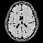
(a) Brain phantom

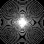
(b) $k$-space sampling mask

Figure 1: (a) shows the brain phantom described in sec:experimental. (b) shows the spiral-shaped $25\%$ $k$-space sub-sampling mask.

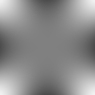
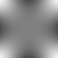
Figure 2: The 36 first spherical basis functions corresponding to $\tilde{n}=5$. For $\tilde{n}=2$ only the 9 first are used.

5.3 Quality measures and parameter selection

All algorithms have been implemented in MATLAB, and the test hardware is an Intel Core i7-6700 HQ CPU 2.60GHz with 8GB RAM. We evaluate the results of the proposed approach in terms of the peak signal-to-noise (PSNR) that is available in the image processing toolbox in MATLAB and the Structural SIMilarity (SSIM) given in [57]. In the computation of the spherical basis function ${f_{l}^{+}}$, we use the Larmour frequency $\omega=42.58$. The conductivity $\sigma$ and the dielectric permittivity $\varepsilon$ are the optimal $(\sigma,\varepsilon)$ for the heterogeneous model in [50] with $\sigma=0.6,\varepsilon=50$. The magnetic permeability for water is $\mu=1.2566\times 10^{-6}$.

5.4 Numerical reconstructions and comparison between (10) and (8)

We perform experiments with the noise level $\tilde{\sigma}=0.05$. We initialize the alg:buildtree1 with $u^{0}=0\in\varmathbb{R}^{N^{2}}$, $a^{0}=(1,\ldots,1)\in{\varmathbb{R}^{Jl_{\max}^{(n)}}}$, and take as step lengths $\tau_{v}^{k}=1/8$, $\tau_{q}^{k}=23$, and $\delta=1/24$ and the remaining $v^{0}$, $\lambda^{0}$, $\bar{\lambda}^{0}$ are all also initialized to zero in the two algorithms. For numerical reconstruction corresponding to (8), we use the codes from [7], available from [6].

We take as regularization parameters $\alpha_{j}=0.4018$, ($j=1,\ldots,J$), $\alpha_{0}=0.0062$ and $\alpha=0.2149$. We perform a fixed number of iterations of alg:buildtree1. With $\tilde{n}=2$, i.e., $l_{\max}=9$, stopping after 1000, 1200, and 1500 iterations, the reconstruction results for the model (10) are shown in fig:5. We also perform the numerical simulations with $\tilde{n}=5$, and the same number of iterations 1000, 1200, and 1500. The reconstruction results for the model (10) are shown in fig:6, and for the model (8) in fig:11. In tab:table6 we report the PNSR and SSIM [57] values. From these results we can observe that the reconstruction quality of the model (10) is much better than the model (8) when iterations are 1000, 1200, and 1500. The reconstruction results can be further improved due to the regularization parameters $\alpha$ not being optimally chosen; for a truly fair comparison of the potential of the two models distinct, parameter learning strategies should be used [16, 17]. What we can with reasonable confidence say based on our experiments here is that the non-linear ADMM converges faster for the model (10) than for (8). This is important in practical applications.

We also report the absolute values of the coefficients $a_{l}^{(j)}$ in tab:table7 when the stopping number of iterations is 1500 for $\tilde{n}=2$. Similarly, tab:table8 shows the absolute values for the resulted coefficients $a_{l}^{(j)}$ for $\tilde{n}=5$ when we stop at 1500 iterations. While for $\tilde{n}=2$ the last rows of the coefficient pyramid for each coil still have high coefficient values, for $\tilde{n}=5$ the coefficients on the last row have decayed to below 1% of the main coefficient on the first row; often 0.1% or less. This supports our starting intuition that a sparse approximation of the coil sensitivities with relatively few coefficients is sufficient for a high-quality reconstruction.

Using the discovered coefficients $a_{l}^{(j)}$, and the known spherical basis functions, we can reconstruct the approximation of the coil sensitivities $c_{j}$. These are in fig:7 and fig:75 for $\tilde{n}=2$ and $\tilde{n}=5$ with 1500 iterations. In order to do the further comparison between (10) and (8), we also give the approximation of $c_{j}$ with 1500 iterations for (8) in fig:79. The PSNR and SSIM values for reconstruction of coils using (10) and (8) for 1500 iterations are reported in tab:table9. Visually, the coil sensitivities constructed with our model (8) are significantly smoother than those constructed with the model (10), and indeed appear to very well approximate the “true” coil sensitivities in fig:2.

To test robustness, we show in fig:9,fig:12 for $\tilde{n}=2$ and $\tilde{n}=5$, respectively, the reconstructions results for the alternative coil sensitivity maps in fig:8. The number of iterations is 1500. The PSNR and SSIM values are reported in tab:table10. Comparing to fig:5,fig:6,tab:table6, we can see that the results remain stable under this perturbation of coil sensitivities, being virtually identical. By contrast, the reconstructed coil sensitivities in fig:10,fig:105 have changed, corresponding to the change in true coil sensitivities.

(a) 1200 iterations

(b) 1500 iterations

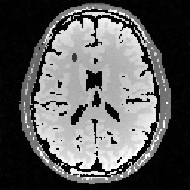
(c) 1800 iterations

Figure 3: Reconstructed brain slice using (10) and $\tilde{n}=2$.

(a) 1200 iterations

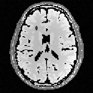
(b) 1500 iterations

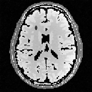
(c) 1800 iterations

Figure 4: Reconstructed brain slice using (10) and $\tilde{n}=5$.

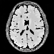
(a) 1200 iterations

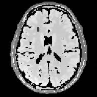
(b) 1500 iterations

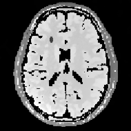
(c) 1800 iterations

Figure 5: Reconstructed brain slice using (8).

Table 6: Reconstruction quality comparison between (10) with $\tilde{n}=2,5$ and (8).

Method	stopping itr. k	PSNR(dB)	SSIM
	1200	25.2750	0.9996
using (10) with $\tilde{n}=2$	1500	25.6878	0.9997
	1800	25.1069	0.9996
	1200	26.0725	0.9997
using (10) with $\tilde{n}=5$	1500	25.5883	0.9997
	1800	25.8730	0.9997
	1200	24.7173	0.9996
using (8)	1500	24.1524	0.9996
	1800	23.6702	0.9995

Table 7: The absolute values of coefficients of $f_{l}^{+}$ with $\tilde{n}=2$ for 1500 iterations. j is the ordinal number of coils.

j	$f_{1}^{+}$
	$f_{2}^{+},f_{3}^{+},f_{4}^{+}$
	$f_{5}^{+},f_{6}^{+},f_{7}^{+},f_{8}^{+},f_{9}^{+}$
	5.4801
1	0.9382, 0.0092, 4.7704
	1.0213, 0.0075, 5.3347, 0.0034, 3.8693
	4.8840
2	0.3632, 0.0059, 4.7055
	1.2463, 0.0085, 4.6682, 0.0083, 4.3803
	3.4124
3	0.2777, 0.0058, 4.3643
	1.7627, 0.0072, 2.2884, 0.0066, 4.1581
	2.6890
4	0.1031, 0.0094, 4.2809
	1.4676, 0.0065, 2.5603, 0.0058, 3.7494

j	$f_{1}^{+}$
	$f_{2}^{+},f_{3}^{+},f_{4}^{+}$
	$f_{5}^{+},f_{6}^{+},f_{7}^{+},f_{8}^{+},f_{9}^{+}$
	3.4487
5	0.2859, 0.0096, 3.6825
	1.1578, 0.0075, 3.1660, 0.0059, 3.2907
	4.3978
6	0.1909, 0.0085, 3.4326
	0.6340, 0.0060, 3.7131, 0.0048, 3.2575
	3.7714
7	0.2415, 0.0016, 3.0790
	1.4061, 0.0070, 4.1169, 0.0045, 3.8595
	3.3760
8	0.2552, 0.0065, 3.2423
	1.6636, 0.0093, 2.7457, 0.0075, 3.7089

Table 8: The absolute values of coefficients of $f_{l}^{+}$ with $\tilde{n}=5$ for 1500 iterations. j is the ordinal number of coils.

	$f_{1}^{+}$
	$f_{2}^{+},f_{3}^{+},f_{4}^{+}$
j	$f_{5}^{+},f_{6}^{+},f_{7}^{+},f_{8}^{+},f_{9}^{+}$
	$f_{10}^{+},f_{11}^{+},f_{12}^{+},f_{13}^{+},f_{14}^{+},f_{15}^{+},f_{16}^{+}$
	$f_{17}^{+},f_{18}^{+},f_{19}^{+},f_{20}^{+},f_{21}^{+},f_{22}^{+},f_{23}^{+},f_{24}^{+},f_{25}^{+}$
	$f_{26}^{+},f_{27}^{+},f_{28}^{+},f_{29}^{+},f_{30}^{+},f_{31}^{+},f_{32}^{+},f_{33}^{+},f_{34}^{+},f_{35}^{+},f_{36}^{+}$
	4.9921
	.6829, .0438, 4.3006
1	.8681,.0165, 5.4029,.0174, 3.9672
	.9972, .0101, 1.9630, .0107, 1.5569, .0051, 5.2987
	.0767, .0075, .0324, .0087, .0344, .0344, .0089, .0135, 5.3953
	.0009, .0085, .0078, .0054, .0242, .0053, .0490, .0074, .0038, .0033, .0069
	4.4692
	.1920, .0465, 4.2089
2	1.2692, .0071, 4.6202, .0165, 4.1568
	.9978, .0050, .0230, .0072, 1.5304, .0038, 4.2382
	.6541, .0098, .0122, .0070, .0428, .0284, .0251, .0071, 5.4117
	.0031, .0075, .0048, .0064, .0066, .0054, .0288, .0059, .0052, .0059, .0040
	3.0346
	.3015, .0392, 3.7538
3	1.6553, .0018, 2.9996, .0041, 4.1566
	.9641, .0057, .3390, .0085, 2.2158, .0087, 3.9728
	.0021, .0080, .0025, .0139, .0255, .0333, .0106, .0030, 4.4230
	.0013, .0075, .0064, .0072, .0030, .0075, .0261, .0075, .0059, .0073, .0048
	2.4995
	.1197, .0360, 3.3852
4	1.4643, .0034, 2.4634, .0056, 3.4846
	1.0066, .0118, .1241, .0061, 1.5655, .0049, 4.3484
	.9035, .0058, .0011, .0142, .0158, .0383, .0126, .0048, 5.1540
	.0043, .0079, .0081, .0076, .0034, .0074, .0268, .0071, .0078, .0080, .0095

	$f_{1}^{+}$
	$f_{2}^{+},f_{3}^{+},f_{4}^{+}$
j	$f_{5}^{+},f_{6}^{+},f_{7}^{+},f_{8}^{+},f_{9}^{+}$
	$f_{10}^{+},f_{11}^{+},f_{12}^{+},f_{13}^{+},f_{14}^{+},f_{15}^{+},f_{16}^{+}$
	$f_{17}^{+},f_{18}^{+},f_{19}^{+},f_{20}^{+},f_{21}^{+},f_{22}^{+},f_{23}^{+},f_{24}^{+},f_{25}^{+}$
	$f_{26}^{+},f_{27}^{+},f_{28}^{+},f_{29}^{+},f_{30}^{+},f_{31}^{+},f_{32}^{+},f_{33}^{+},f_{34}^{+},f_{35}^{+},f_{36}^{+}$
	3.1244
	.2371, .0362, 3.0439
5	.9841, .0108, 3.2107, .0073, 2.8668
	.8269, .0041, .0164, .0065, .5001, .0153, 4.3171
	.0811, .0057, .0055, .0057, .0239, .0266, .0237, .0025, 4.6823
	.0025, .0061, .0072, .0077, .0125, .0088, .0353, .0091, .0052, .0111, .0058
	3.9430
	.3079, .0451, 3.1557
6	.6159, .0090, 4.0539, .0148, 2.8496
	1.3257, .0072, .0080, .0128, 1.5127, .0052, 3.1355
	.3157, .0061, .0212, .0080, .0327, .0422, .0358, .0122, 4.5738
	.0047, .0071, .0085, .0083, .0087, .0076, .0341, .0062, .0099, .0074, .0064
	3.4755
	.2479, .0338, 2.9170
7	1.3750, .0061, 3.7187, .0110, 3.4468
	.8354, .0115, .1450, .0138, 1.4890, .0046, 3.9267
	.0038, .0074, .0169, .0107, .0299, .0389, .0244, .0157, 4.2940
	.0028, .0078, .0054, .0075, .0021, .0071, .0275, .0055, .0043, .0068, .0051
	2.9650
	.2303, .0268, 2.9961
8	1.5204, .0118, 3.1554, .0206, 3.4432
	1.3120, .0106, .1190, .0056, 1.3044, .0064, 4.4748
	.6673, .0071, .0079, .0051, .0222, .0196, .0165, .0123, 4.9405
	.0031, .0080, .0065, .0070, .0114, .0076, .0177, .0087, .0153, .0102, .0076

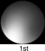
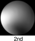
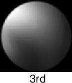
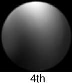
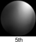
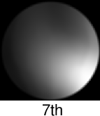
Figure 6: Coil sensitivities generated by the measurements of a water bottle with 8-channel head coil array.

Figure 7: Reconstructed coil sensitivities for the 8 different coils when the number of iterations is 1500 for $\tilde{n}=2$.

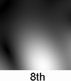
Figure 8: Reconstructed coil sensitivities for the 8 different coils when the number of iterations is 1500 for $\tilde{n}=5$.

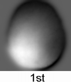
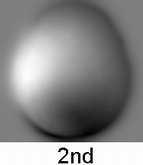
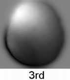
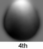
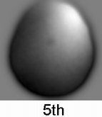
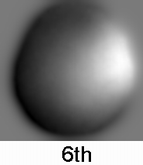
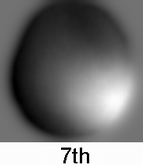
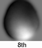
Figure 9: Reconstructed coil sensitivities for the 8 different coils when the number of iterations is 1500 for (8).

(a) 1200 iterations

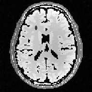
(b) 1500 iterations

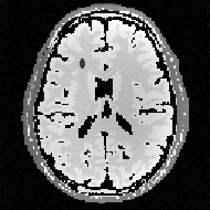
(c) 1800 iterations

Figure 10: Reconstruction when data is generated with the alternative coil sensitivities from fig:8 with $\tilde{n}=2$.

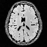
(a) 1200 iterations

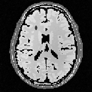
(b) 1500 iterations

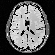
(c) 1800 iterations

Figure 11: Reconstruction when data is generated with the alternative coil sensitivities from fig:8 with $\tilde{n}=5$.

Table 9: Reconstruction quality comparison between (10) with $\tilde{n}=2,5$ and (8) for 1500 iterations.

Method	coil No.	PSNR(dB)	SSIM
	coil 1	8.5038	0.9864
	coil 2	8.9329	0.9878
	coil 3	8.9895	0.9873
	coil 4	10.7526	0.9918
using (10) with $\tilde{n}=2$	coil 5	10.2633	0.9900
	coil 6	10.6595	0.9917
	coil 7	9.0644	0.9869
	coil 8	11.2573	0.9929
	coil 1	7.2807	0.9849
	coil 2	8.2247	0.9878
	coil 3	7.4537	0.9850
	coil 4	9.3979	0.9903
using (10) with $\tilde{n}=5$	coil 5	9.1837	0.9891
	coil 6	10.3233	0.9919
	coil 7	8.5967	0.9876
	coil 8	10.1097	0.9920
	coil 1	5.9826	0.9759
	coil 2	5.9328	0.9754
	coil 3	5.9124	0.9748
	coil 4	6.3114	0.9779
using (8)	coil 5	6.1844	0.9762
	coil 6	6.1754	0.9765
	coil 7	6.3423	0.9772
	coil 8	6.4319	0.9774

Table 10: The PSNR and SSIM values for reconstruction with alternative coil sensitivities using (10) with $\tilde{n}=2$ and $\tilde{n}=5$

Method	stopping itr. k	PSNR(dB)	SSIM
	1200	27.0202	0.9998
using (10) with $\tilde{n}=2$	1500	24.2239	0.9995
	1800	24.9633	0.9996
	1200	30.8382	0.9999
using (10) with $\tilde{n}=5$	1500	30.7620	0.9999
	1800	30.6448	0.9999

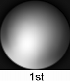
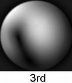
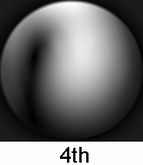
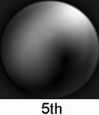
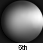
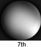
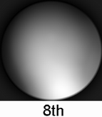
Figure 12: Alternative Perturbed coil sensitivity maps.

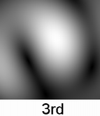
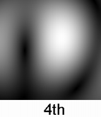
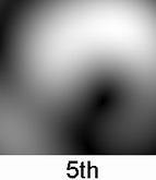
Figure 13: Reconstructed coil sensitivities when data is generated with the alternative coil sensitivities from fig:8. The number of iterations is 1500 and $\tilde{n}=2$.

Figure 14: Reconstructed coil sensitivities when data is generated with the alternative coil sensitivities from fig:8. The number of iterations is 1500 and $\tilde{n}=5$.

6 Conclusions

In this paper, we have established a new model for parallel MRI reconstruction based on sparse regularization of coil sensitivities in spherical basis function bases. We have developed efficient recurrence formulas for the computation of these functions. We have then applied the non-linear ADMM from [7] to numerically solve our model (10). By numerical reconstructions and comparison between (10) and (8), we think that the reconstruction quality for proposed model (10) is better than the model (8). In additional, the reconstruction for our model (10) for the alternative coils sensitivity maps is very robust. That has an important significance in practical applications. In the future, we will study the optimal choice among the regularization parameters $\alpha_{j}$, $\alpha_{0}$, and $\alpha$ to improve reconstruction quality furthermore via parameter learning strategies in [16, 17].

A data statement for the EPSRC

All data and source codes will be publicly deposited when the final accepted version of the manuscript is submitted.

References

- [1] G.. Arfken and H.. Weber “Mathematical methods for physicists” San Diego: Hartcourt/Academic Press, 2001
- [2] K.. Arrow, L. Hurwicz and H. Uzawa “Studies in Linear and Non-Linear Programming” Stanford: Stanford University Press, 1958
- [3] B. Aubert-Broche, A.. Evans and L. Collins “A new improved version of realistic digital brain phantom” In NeuroImage 32.1, 2006, pp. 138–145
- [4] A.. Bakushinsky and M.. Kokurin “Iterative methods for approximate solution of inverse problems”, Mathematics and its Applications Vol. 577. Springer, 2004
- [5] F. Bauer and S. Kannengiesser “An Alternative Approach to the Image Reconstruction for Parallel Data Acquisition in MRI” In Math Meth Appl Sci. 30.12, 2007, pp. 1437–1451
- [6] M. Benning, F. Knoll, C.. Schönlieb and T. Valkonen “Research data supporting: Preconditioned ADMM with nonlinear operator constraint”, 2016 DOI: 10.17863/CAM.163
- [7] Martin Benning, Florian Knoll, Carola-Bibiane Schönlieb and Tuomo Valkonen “Preconditioned ADMM with Nonlinear Operator Constraint” In System Modeling and Optimization: 27th IFIP TC 7 Conference, CSMO 2015, Sophia Antipolis, France, June 29–July 3, 2015, Revised Selected Papers Springer International Publishing, 2016, pp. 117–126 DOI: 10.1007/978-3-319-55795-3_10
- [8] M.. Bernstein, K.. King and X.. Zhou “Handbook of MRI Pulse Sequences” Elsevier, 2004
- [9] B. Blaschke, A. Neubauer and O. Scherzer “On convergence rates for the iteratively regularized Gauss-Newton method” In IMA J Numer Anal. 17.3, 1997, pp. 421–436
- [10] K. Bredies, K. Kunisch and T. Pock “Total generalized variation” In SIAM J. on Imaging Sci. 3.3, 2010, pp. 492–526
- [11] M. Bydder, D.. Larkman and J.. Hajnal “Generalized SMASH Imaging” In Magn. Reson. Med. 47.1, 2002, pp. 160–170
- [12] A. Chambolle “An algorithm for total variation minimization and applications” In J. Math. Imag. Vis. 20.1-2, 2004, pp. 89–97
- [13] D.. Cheng “Time varying fields and Maxwell’s equations. In: Cheng DK. Field and Wave Electromagnetics” Chevy Chase, MD:Addison-Wesley, 1989
- [14] Christian Clason and Tuomo Valkonen “Primal-dual extragradient methods for nonlinear nonsmooth PDE-constrained optimization” In SIAM Journal on Optimization 27.3, 2017, pp. 1313–1339
- [15] P.. Combettes and V.. Wajs “Signal recovery by proximal forward-backward splitting” In Multiscale Model. Simul. 4.4, 2005, pp. 1168–1200
- [16] Juan Carlos Los Reyes and Carola-Bibiane Schönlieb “Image denoising: Learning noise distribution via PDE-constrained optimization” In Inverse Problems and Imaging 7, 2013, pp. 1183–1214 arXiv:1207.3425
- [17] Juan Carlos Los Reyes, Carola-Bibiane Schönlieb and Tuomo Valkonen “Bilevel parameter learning for higher-order total variation regularisation models” In Journal of Mathematical Imaging and Vision 57, 2017, pp. 1–25 DOI: 10.1007/s10851-016-0662-8
- [18] A.. Devaney “Multipole expansion and plane wave representations of the electromagnetic field” In J. Math. Phys. 15.2, 1974, pp. 234–244
- [19] H.. Engl, M. Hanke and A. Neubauer “Regularization of inverse problems”, Mathematics and its Applications Vol. 375. Kluwer Academic Publishers Group, 1996
- [20] Ernie Esser, Xiaoqun Zhang and Tony F Chan “A general framework for a class of first order primal-dual algorithms for convex optimization in imaging science” In SIAM Journal on Imaging Sciences 3.4 SIAM, 2010, pp. 1015–1046 DOI: 10.1137/09076934X
- [21] D. Gabay “Applications of the method of multipliers to variational inequalities. In: Augmented Lagrangian Methods:Applications to the Solution of Boundary-Value Problems” Amsterdam: North-Holland, 1983
- [22] M.. Griswold et al. “Generalized Autocalibrating Partially Parallel Acquisitions (GRAPPA)” In Magn. Reson. Med. 47.6, 2002, pp. 1202–1210
- [23] M.. Griswold et al. “Autocalibrated Coil Sensitivity Estimation for Parallel Imaging” In NMR Biomed 19.3, 2006, pp. 316–324
- [24] W.. Hoge, D.. Brooks, B. Maddore and W.. Kyriakos “A Tour of Accelerated Parallel MR Imaging from A Linear Systems Perspective” In Concepts Magn Reson Part A 27.1, 2005, pp. 17–37
- [25] W.. Hoge, D.. Brooks, B. Madore and W. Kyriakos “On the regularization of SENSE and space-RIP in parallel MR imaging” In Proc. IEEE Int Biomedical Imaging: Nano to Macro Symp. 51.3, 2004, pp. 241–244
- [26] T. Hohage “Logarithmic Convergence Rates of the Iteratively Regularized Gauss-Newton Method for an Inverse Potential and an Inverse Scattering Problem” In Inverse Problems 13.5, 1997, pp. 1279–1299
- [27] D.. Hoult “The Principle of Reciprocity in Signal Strength Calculations-A Mathematical Guide” In Concepts Magn Reson Part A 12.4, 2000, pp. 173–187
- [28] M. Hutchinson and U. Raff “Fast MRI Data Acquisition Using Multiple Detectors” In Magn. Reson. Med. 6.1, 1988, pp. 87–91
- [29] T.. Ibrahim “Analytical approach to the MR Signal” In Magn. Reson. Med. 54.3, 2005, pp. 677–682
- [30] J. Jin et al. “An Electromagnetic reverse method of coil sensitivity mapping for parallel MRI-theoretical framework” In J. Magn. Reson. 207.1, 2010, pp. 59–68
- [31] D.. Jones “Acoustic and electromagnetic waves” New York: Oxford University Press, 1989
- [32] J.. Kelner et al. “Electromagnetic fields of surface coil in vivo NMR at high frequencies” In Magn. Reson. Med. 22.2, 1991, pp. 467–480
- [33] F. Knoll, K. Bredies, T. Pock and R. Stollberger “Second Order Total Generalized Variation (TGV) for MRI” In Magn. Reson. Med. 65.2, 2011, pp. 480–491
- [34] F. Knoll, C. Clason, M. Uecker and R. Stollberger “Improved Reconstruction in Non-cartesian Parallel Imaging by Regularized Nonlinear Inversion” Honolulu, HI: Proceedings of the 17th Scientific MeetingExhibition of ISMRM, 2009
- [35] F. Knoll et al. “Parallel Imaging with Nonlinear Reconstruction using Variational Penalties” In Magn. Reson. Med. 67.1, 2012, pp. 34–41
- [36] W.. Kyriakos et al. “Sensitivity Profiles from An Array of Coils for Encoding and Reconstruction in Parallel (SPACE RIP)” In Magn. Reson. Med. 44.2, 2000, pp. 301–308
- [37] D.. Larkman and R.. Nunes “Parallel Magnetic Resonance Imaging” In Phys. Med. Biol. 52.7, 2007, pp. R15–R55
- [38] B. Lemaire “in International Series of Numberical Mathematics” Basel, Switzerland: Birkhäuser-Verlag, 1989, pp. 73–87
- [39] F.. Lin, K.. Kwong, J.. Belliveau and L.. Wald “Parallel imaging reconstruction using automatic regularization” In Magn. Reson. Med. 51.3, 2004, pp. 559–567
- [40] B. Martinet “Pertubation des methodes d’optimisation: Application” In RAIRO Anal. Numer. 12.2, 1978, pp. 153–171
- [41] C.. McKenzie et al. “Self-calibrating Parallel Imaging with Automatic Coil Sensitivity Extraction” In Magn. Reson. Med. 47.3, 2002, pp. 529–538
- [42] J.. Moreau “Proximit et dualite dans un espace Hilbertien” In Bull. Soc. Math. France 93, 1965, pp. 273–299
- [43] O. Ocali and E. Atalar “Ultimate intrinsic signal-to-noise ratio in MRI” In Magn. Reson. Med. 39.3, 1998, pp. 462–473
- [44] K.. Pruessmann “Sensitivity Encoded Magnetic Resonance Imaging, Ph. D. thesis” Zurich: Swiss Federal Insititute of Technology, 2000
- [45] K.. Pruessmann, M. Weiger, P. Bornert and P. Boesiger “Advances in Sensitivity Encoding with Arbitrary k-Space Trajectories” In Magn. Reson. Med. 46.4, 2001, pp. 638–651
- [46] K.. Pruessmann, M. Weiger, M.. Scheidegger and P. Boesiger “SENSE: Sensitivity Encoding for Fast MRI” In Magn. Reson. Med. 42.5, 1999, pp. 952–962
- [47] R.. Rockafellar “Augmented Lagrangians and applications of the proximal point algorithm in convex programming” In Math. Oper. Res. 1.2, 1976, pp. 97–116
- [48] R.. Rockafellar “Monotone operators and the proximal point algorithm” In SIAM J. Control Optim. 14.5, 1976, pp. 877–898
- [49] L.. Rudin, S.. Osher and E. Fatemi “Nonlinear total variation based noise removal algorithm” In Phys. D 60.1-4, 1992, pp. 259–268
- [50] A. Sbrizzi et al. “Robust reconstruction of maps by projection into a spherical functions space” In Magn. Reson. Med. 71.1, 2014, pp. 394–401
- [51] D.. Sodickson and W.. Manning “Simulataneous Acquisition of Spatial Harmonics (SMASH): Fast Imaging with Radiofrequency Coil Arrays” In Magn. Reson. Med. 38.4, 1997, pp. 591–603
- [52] M. Uecker, T. Hohage, K.. Block and J. Frahm “Image Reconstruction by Regularized Nonlinear Inversion-Joint Estimation of Coil Sensitivities and Image Content” In Magn. Reson. Med. 60.3, 2008, pp. 674–682
- [53] M. Uecker, A. Karaus and J. Frahm “Inverse Reconstruction Method for Segmented Multishot Diffusion-weighted MRI with Multiple Coils” In Magn. Reson. Med. 62.5, 2009, pp. 1342–1348
- [54] T. Valkonen “A primal-dual hybrid gradient method for non-linear operators with applications to MRI” In Inverse Problems 30.5, 2014 DOI: 10.1088/0266-5611/30/5/055012
- [55] T. Valkonen “Testing and non-linear preconditioning of the proximal point method”, 2017 URL: https://arxiv.org/abs/1703.05705v2
- [56] T. Valkonen, K. Bredies and F. Knoll “Total generalized variation in diffusion tensor imaging” In SIAM J. on Imaging Sci. 6.1, 2013, pp. 487–525
- [57] Z. Wang, A.. Bovik, H.. Sheikh and E.. Simoncelli “Image quality assessment: From error visibility to structural similarity” In IEEE Transactions on Image Processing 13.4, 2004, pp. 600–612 DOI: 10.1109/TIP.2003.819861
- [58] F. Wiesinger, P. Boesiger and K.. Pruessmann “Electrodynamics and ultimate SNR in parallel MR imaging” In Magn. Reson. Med. 52.2, 2004, pp. 376–390
- [59] L. Ying and J. Sheng “Joint Image Reconstruction and Sensitivity Estimation in SENSE (JSENSE)” In Magn. Reson. Med. 57.6, 2007, pp. 1196–1202
- [60] X. Zhang, M. Burger and S. Osher “A unified primal-dual algorithm framework based on Bregman iteration” In J Sci Comput 46.1, 2011, pp. 20–46
- [61] Xiaoqun Zhang, Martin Burger and Stanley Osher “A Unified Primal-Dual Algorithm Framework Based on Bregman Iteration” In Journal of Scientific Computing 46.1, 2011, pp. 20–46 DOI: 10.1007/s10915-010-9408-8
- [62] Y. Zhu “Parallel Excitation with An Array of Transmit Coils” In Magn. Reson. Med. 51.4, 2004, pp. 775–784
- [63] Y. Zhu and Y. Shi “A Fast Method for Reconstruction of Total-Variation MR Images With a Periodic Boundary Condition” In IEEE Signal Processing Letters 20.4, 2013, pp. 291–294
- [64] Y. Zhu, Y. Shi, B. Zhang and X. Yu “Weighted-average Alternating Minimization Method For Magnetic Resonance Image Reconstruction Based On Compressive Sensing” In Inverse Problems and Imaging 8.3, 2014, pp. 925–935