Universal Quantum Noise in Adiabatic Pumping

Abstract

We consider charge pumping in a system of parafermions, implemented at fractional quantum Hall edges. Our pumping protocol leads to a noisy behavior of the pumped current. As the adiabatic limit is approached, not only does the noisy behavior persist but the counting statistics of the pumped current becomes robust and universal. In particular, the resulting Fano factor is given in terms of the system’s topological degeneracy and the pumped quasiparticle charge. Our results are also applicable to the more conventional Majorana fermions.

Adiabatic quantum pumping, first introduced by Thouless Thouless (1983), is a powerful instrument in studying properties of quantum systems. The underlying physics can be related to the system’s Berry phase Thouless (1983), disorder configurations Spivak et al. (1995), scattering matrix and transport Brouwer (1998), critical points Sela and Oreg (2006), and topological properties Fu and Kane (2006); Kraus et al. (2012); Keselman et al. (2013); Marra et al. (2015). In many cases Thouless (1983); Sela and Oreg (2006); Fu and Kane (2006); Kraus et al. (2012); Keselman et al. (2013); Marra et al. (2015), adiabatic pumping is noiseless at zero temperature, as the same number of quanta (of charge, spin, etc.) is pumped every cycle and the pumping precision is increased (the noise vanishes) as the adiabatic limit is approached. On the other hand, noisy adiabatic quantum pumps are known and have been extensively studied Andreev and Kamenev (2000); Avron et al. (2001); Makhlin and Mirlin (2001); Moskalets and Büttiker (2002, 2004); Riwar et al. (2013). The simplest (and a typical) example of such a noisy pump is two reservoirs of electrons connected by a junction described by a scattering matrix. As the phase of the reflection amplitude $r$ is varied from $0$ to $2\pi$, an electron is pumped with probability $|r|^{2}$ Andreev and Kamenev (2000). The probabilistic nature of the adiabatic pumping process relies on the degeneracy of scattering states. The pumped current and its noise are sensitive to $|r|$, which in turn is highly sensitive to the system parameters. In fact, in all such examples Andreev and Kamenev (2000); Avron et al. (2001); Makhlin and Mirlin (2001); Moskalets and Büttiker (2002, 2004); Riwar et al. (2013), the pumped current and its noise depend on the details of the pumping cycle and/or of coupling the system to external leads.

In this Letter, we implement the concept of adiabatic pumping to a setup of topological matter. We find that, when the adiabatic limit is approached, not only is the pumped current noisy (a manifestation of the degeneracy of the underlying Hilbert space), but it is also universal: the current and its noise become largely independent of the specific parameters used in the pumping cycle, and the related Fano factor is directly related to the underlying topological structure; cf. Eq. (1). Before going into technical details, we now summarize the essence and the physical origin of our findings.

Qualitative overview of our protocol.—The topological system underlying our adiabatic pump is an array of parafermions (PFs), depicted in Fig. 1a. Consider an example of the system employing fractional quantum Hall (FQH) puddles of filling factor $\nu=1/3$. Each of the superconducting (SC) domains, $\mathrm{SC}_{i}$, is characterized by the fractional component of its charge $Q_{i}/e=(0,1/3,2/3,...,5/3)$, defined modulo $2e$ as charge quanta of $2e$ can be absorbed by the proximitizing SC. Each of the two SC domains in Fig. 1a thus has $d=6$ states . The system’s topological nature renders the states of different $Q_{i}$ degenerate, leading to $d^{2}$-degenerate Hilbert space. Let us now consider a coherent source that is capable of injecting FQH quasiparticles (QPs) of charge $e^{*}=e/3$ into $\mathrm{SC}_{1}$. As the coherent source of QPs, we employ a quantum antidot (QAD) Kivelson and Pokrovsky (1989); Kivelson (1990); Goldman and Su (1995); Goldman (1997); Maasilta and Goldman (1997), which is a depleted region in the FQH incompressible puddle that can host fractional QPs. At low energies, this injection can take place only at domain walls between $\mathrm{SC}_{1}$ and the neighboring $\mathrm{FM}$ domains. As a result of such an injection, $Q\equiv Q_{1}$ would change $Q\rightarrow(Q+1/3)\thinspace\mathrm{\mod\thinspace 2}$. The two trajectories of injection (through the left or the right domain wall) interfere with each other, implying that the probability of a successful injection may be smaller than $1$ (and even tuned to 0). The latter, $P(Q)$, depends on the domain charge $Q$. $\mathrm{QAD}_{1}$ used for the injection of QPs into $\mathrm{SC}_{1}$ is denoted as 1 in Fig. 1a.

It turns out that in the limit of adiabatic manipulation with the QAD parameters, $P(Q)$ can be either $0$ when the interference is fully destructive or $1$ otherwise [see the discussion after Eq. (12)]. By tuning $P(Q=Q_{\mathrm{B}})=0$ for one of the system states $Q_{\mathrm{B}}$, while $P(Q\neq Q_{\mathrm{B}})=1$, one blockades the repeated injection of QPs as shown in Fig. 1b: starting from any state, the system eventually arrives in $Q=Q_{\mathrm{B}}$, stopping any further injection of quasiparticles. We dub this phenomenon a topological pumping blockade .

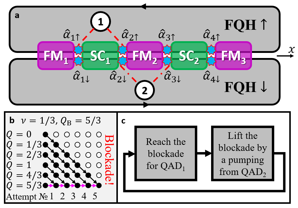
Figure 1: a — The system layout. In the regions proximitized by ferromagnets (FM) and superconductors (SC), the FQH edges (of opposite spin FQH puddles each of the same filling factor $\nu$) are gapped out in two respective distinct ways. Each domain wall between a SC and a FM region hosts PF zero mode operators (blue stars). The free edges of spin-$\uparrow$ and spin-$\downarrow$ parts are glued together by total reflection at the FMs. The bulk of the FQH puddles hosts quantum anti-dots (QADs, denoted as 1 and 2) — regions depleted by local gates. QADs behave as local enclaves that can support FQH QPs. Tunnel couplings (red dashed and dot-dashed lines) between QADs and parafermionic domain walls allow QPs to tunnel between them, influencing the state of the PFs. All the proximitizing SCs (FMs) are implied to be parts of a single bulk SC (FM), respectively. b — The mechanism of $\mathrm{QAD}_{1}$ pumping blockade. Under repeated pumping attempts, the system eventually reaches the state of $\mathrm{SC}_{1}$ domain charge $Q=0$, in which pumping is blockaded. c — The elementary cycle of the protocol producing universal pumping noise.

We now employ an additional QAD ($\mathrm{QAD}_{2}$, denoted as 2 in Fig. 1a) for lifting the blockade. A QP from $\mathrm{QAD}_{2}$ may be injected to either the second or the third domain wall. In the former case it would change the $\mathrm{SC}_{1}$ charge $Q_{\mathrm{B}}\rightarrow(Q_{\mathrm{B}}+1/3)\thinspace\mathrm{\mod\thinspace 2}$, allowing for several more successful injections from $\mathrm{QAD}_{1}$, while in the latter case the QP is injected to $\mathrm{SC}_{2}$, leaving $Q$ unchanged. The probability of each outcome is governed by the QP tunneling amplitude from $\mathrm{QAD}_{2}$ to the respective domain wall. Consider a protocol whose elementary cycle consists of $d-1$ QP injection attempts from $\mathrm{QAD}_{1}$ (sufficiently many to reach the blockade irrespectively of the system initial state) followed by disconnecting $\mathrm{QAD}_{1}$ from the array, then a single injection from $\mathrm{QAD}_{2}$, and finally disconnecting $\mathrm{QAD}_{2}$; cf. Fig. 1c. Then in each cycle the number of qps successfully injected from $\mathrm{QAD}_{1}$ is determined by the value of $Q$ at the beginning of the cycle and should therefore be either 0 or 5 with the corresponding probabilities.

A more careful consideration, however, shows that the mere connection of $\mathrm{QAD}_{2}$ to the two domain walls simultaneously allows for transfer of QPs between $\mathrm{SC}_{1}$ and $\mathrm{SC}_{2}$: a QP can jump (through a virtual or a real process) from one domain wall to the QAD and then to the other domain wall. As a result, any state $Q$ at the beginning of the cycle is possible. For example, if the QP from $\mathrm{QAD}_{2}$ is injected to $\mathrm{SC}_{1}$ and on top of that $k$ QPs are transferred from $\mathrm{SC}_{2}$ to $\mathrm{SC}_{1}$, then $Q_{\mathrm{B}}\rightarrow\left(Q_{\mathrm{B}}+(k+1)/3\right)\thinspace\mathrm{\mod\thinspace 2}$. Moreover, transfers of $k$ and $k+d$ QPs lead to the same value of $Q$, and, therefore, these processes interfere. The interference phases of these processes are sensitive to such parameters as the strength of tunneling amplitudes between $\mathrm{QAD}_{2}$ and the domain walls, the QAD potential, or the duration of the injection process. In the adiabatic limit, a tiny cycle-to-cycle variation of these parameters leads to a strong variation of the interference phases. Therefore, averaged over many pumping cycles, the probability of starting the cycle in any of the $d$ possible states $Q$ is the same and is equal to $1/d$. The average current of charge pumped from $\mathrm{QAD}_{1}$ into the array, $I$, and its zero-frequency noise $S$, are then given, respectively, by

$$I=I_{0}\frac{d-1}{2d},\quad S=\frac{d+1}{6}e^{*}I,$$ (1)

where $I_{0}=e^{*}/\tau$ and $\tau$ is the duration of a single injection attempt.

The model. Parafermions.—Following Refs. Lindner et al. (2012); Clarke et al. (2013), we consider a parafermion array realized on the boundary of two $\nu=1/(2p+1)$ FQH puddles, consisting of electrons of opposite spin; cf. Fig. 1a. The dynamics of the respective FQH edges is described by fields $\hat{\phi}_{s}(x)$, $s=\pm 1=\uparrow/\downarrow$, satisfying $[\hat{\phi}_{s}(x),\hat{\phi}_{s}(y)]=i\pi s\mathrm{sgn}(x-y)$ and $[\hat{\phi}_{\uparrow}(x),\hat{\phi}_{\downarrow}(y)]=i\pi$ Clarke et al. (2013). The edges support domains that are gapped by proximity coupling to a superconductor (SC) or a ferromagnet (FM); $H=H_{\mathrm{edge}}+H_{\mathrm{SC}}+H_{\mathrm{FM}}$, where $H_{\mathrm{edge}}=(v/4\pi)\int_{0}^{L}dx\left[(\partial_{x}\hat{\phi}_{\uparrow})^{2}+(\partial_{x}\hat{\phi}_{\downarrow})^{2}\right]$ with edge velocity $v$,

$$H_{\mathrm{SC}} = -\frac{\Delta}{a}\sum_{j=1}^{N}\int_{\mathrm{SC}_{j}}dx\cos\left(\frac{\hat{\phi}_{\uparrow}(x)+\hat{\phi}_{\downarrow}(x)}{\sqrt{\nu}}\right),$$ (2)

$$H_{\mathrm{FM}} = -\frac{\mathcal{M}}{a}\sum_{j=1}^{N+1}\int_{\mathrm{FM}_{j}}dx\cos\left(\frac{\hat{\phi}_{\uparrow}(x)-\hat{\phi}_{\downarrow}(x)}{\sqrt{\nu}}\right),$$ (3)

with $\Delta$ (respectively, $\mathcal{M}$) being the absolute value of the induced amplitude for SC pairing (for tunneling between edge segments proximitized by FMs), short-distance cutoff $a$, and $N=2$ is the number of SC domains. All the proximitizing SCs (FMs) are implied to be parts of a single bulk SC (FM), respectively. The bulk SC is assumed to be grounded. For $\Delta a/v$, $\mathcal{M}a/v>\sqrt{2\nu-\ln 2\nu-1}/(2\sqrt{2}\pi\nu^{2})$ when $\nu\leq 1/3$ and for any nonzero values of $\Delta a/v$ and $\mathcal{M}a/v$ when $\nu=1$, each domain has a gap for QP excitations. At low energies, each domain can be described by a single integer-valued operator Lindner et al. (2012); Clarke et al. (2013)

$$\left.\frac{\hat{\phi}_{\uparrow}(x)\mp\hat{\phi}_{\downarrow}(x)}{2\pi\sqrt{\nu}}\right|_{x\in\mathrm{FM}_{j}/\mathrm{SC}_{j}}=\left\{\begin{array}[]{c}\hat{m}_{j},\\ \hat{n}_{j}.\end{array}\right.$$ (4)

The only nontrivial commutation relation is $[\hat{m}_{j},\hat{n}_{l}]=i/(\pi\nu)$ for $j>l$, while $[\hat{m}_{j},\hat{n}_{l}]=0$ for $j\leq l$. Being integer-valued noncommuting operators, they are defined modulo $d=2/\nu$, i.e., $\hat{m}_{j}\thinspace(\hat{n}_{j})\sim\hat{m}_{j}\thinspace(\hat{n}_{j})+d$. The fractional component of the $j^{\mathrm{th}}$ SC domain’s charge $\hat{Q}_{j}$ is given by $\hat{Q}_{j}\thinspace\mathrm{mod}\thinspace 2e=e^{*}(\hat{m}_{j+1}-\hat{m}_{j})\thinspace\mathrm{mod}\thinspace 2e=\nu\left[(\hat{m}_{j+1}-\hat{m}_{j})\thinspace\mathrm{mod}\thinspace d\right]$, where $e^{*}=\nu e$ and $e$ are, respectively, the charge of the fractional QP and the electron charge, and we put $e=1$. The parafermion array Hilbert space may be spanned by states $|m_{1},Q,m_{3}\rangle$, where $m_{j}$ is the eigenvalue of $\hat{m}_{j}$ and $Q$ is the eigenvalue of $(\hat{Q}_{1}\thinspace\mathrm{mod}\thinspace 2e)$. Alternatively, one can use the basis of $|m_{1},S,m_{3}\rangle$ with $S$ being the eigenvalue of $\nu\left[(\hat{n}_{1}-\hat{n}_{2})\thinspace\mathrm{mod}\thinspace d\right]$. The possible values for both $Q$ and $S$ are $0,\nu,...,(d-1)\nu\equiv 2-\nu$ . These two bases are related as

$$|m_{1},S,m_{3}\rangle=\frac{1}{\sqrt{d}}\sum_{Q=0}^{(d-1)\nu}e^{i\pi dQS/2}|m_{1},Q,m_{3}\rangle.$$ (5)

Our protocols involve tunneling fractional QPs into the parafermion array. At low energies such tunneling may take place only at the interfaces between different domains. The low-energy projection of the QP operators is given by (cf. Refs. Lindner et al. (2012); Clarke et al. (2013))

$$\hat{\alpha}_{js}=\left\{\begin{array}[]{cc}e^{i\pi\nu(\hat{n}_{l}+s\hat{m}_{l})},&j=2l-1,\\[2.84544pt] e^{i\pi\nu(\hat{n}_{l}+s\hat{m}_{l+1})},&j=2l,\end{array}\right.,$$ (6)

where $j$ is the domain wall number and $s=\pm 1=\uparrow/\downarrow$ is the spin of the edge into which the QP tunnels. For $\nu=1$, $\hat{\alpha}_{js}$ become Majorana fermions.

In addition to the parafermion-hosting domain walls, quantum antidots are the second main ingredient of our model. We consider small QADs in the Coulomb blockade regime. Such a QAD can be modeled as a system of two levels, $|q\rangle$ and $|q+\nu\rangle$, corresponding to the QAD hosting charge $q$ or $q+\nu$ respectively. The QP operator on the QAD and the QAD Hamiltonian assume then the forms

$$\hat{\psi}_{\mathrm{QAD}}=\begin{pmatrix}0&0\\ 1&0\end{pmatrix},$$ (7)

$$H_{\mathrm{QAD}}=\nu V_{\mathrm{QAD}}\left(\hat{\psi}_{\mathrm{QAD}}^{\dagger}\hat{\psi}_{\mathrm{QAD}}^{\thinspace}-\frac{1}{2}\right)=\frac{V_{\mathrm{QAD}}}{d}\begin{pmatrix}1&0\\ 0&-1\end{pmatrix},$$ (8)

where $V_{\mathrm{QAD}}$ is an electrostatic gate potential. One can consider several QADs, each described by such a two-level Hamiltonian .

The Hamiltonian describing tunneling of QPs between a QAD and the PF system is

$$H_{\mathrm{tun}}=\sum_{j}\eta_{js}\hat{\psi}_{\mathrm{QAD},s}^{\thinspace}\hat{\alpha}_{js}^{\dagger}+\mathrm{H.c.}$$ (9)

Here $\eta_{js}$ is the tunneling amplitude to the $j^{\mathrm{th}}$ domain wall, and $\hat{\alpha}_{js}$ is the PF operator in this domain wall. Fractional QPs can tunnel only through a FQH bulk but not through a vacuum. The QAD is embedded in the FQH puddle of spin $s$ and is therefore coupled only to the PFs of the same spin; this is indicated by index $s$ of the QAD operator.

Injection of a QP from $\mathrm{QAD}_{1}$.—In Fig. 1a, $\mathrm{QAD}_{1}$ is connected to parafermions $\hat{\alpha}_{1\uparrow}$ and $\hat{\alpha}_{2\uparrow}$. The tunneling Hamiltonian (9) then allows for transitions only between states $|q+\nu\rangle_{\mathrm{QAD}_{1}}|m_{1},Q,m_{3}\rangle\equiv|1\rangle$ and $|q\rangle_{\mathrm{QAD}_{1}}|m_{1},Q+\nu,m_{3}+1\rangle\equiv|0\rangle$. The problem of QP tunneling can therefore be mapped onto a set of $2\times 2$ problems each described by the Hamiltonian

$$H_{\mathrm{LZ}}(t)=\begin{pmatrix}\frac{1}{d}V_{\mathrm{QAD}}(t)&\eta_{Q}^{*}\\ \eta_{Q}&-\frac{1}{d}V_{\mathrm{QAD}}(t)\end{pmatrix},$$ (10)

$$\eta_{Q}=e^{-i\pi\nu m_{1}}\left(\eta_{1\uparrow}+\eta_{2\uparrow}e^{-i\pi\left(Q+\frac{\nu}{2}\right)}\right).$$ (11)

For this Hamiltonian, consider the Landau-Zener problem LZ_ ; Landau and Lifshitz (1977): $V_{\mathrm{QAD}}(t)=\nu^{-1}\lambda t$ with $\lambda>0$; at $t=-T$ the effective two-level system is prepared in the lower-energy state $|\psi(-T)\rangle=|1\rangle$ ($|1\rangle$ and $|0\rangle$ are the diabatic states of the QAD–PF system). Then at $t=+T$ it will generally be in a superposition of the two diabatic states. When $T\rightarrow+\infty$, the probability of staying in state $|1\rangle$ (i.e., not injecting the QP) is

$$P_{\mathrm{LZ}}=\exp\left(-2\pi\gamma\right),$$ (12)

where $\gamma=|\eta_{Q}|^{2}/\lambda$. Unless $\eta_{Q}=0$, the probability $P(Q)=1-P_{\mathrm{LZ}}$ of switching from $|1\rangle$ to $|0\rangle$, i.e., of injecting a QP to $\mathrm{SC}_{1}$ domain, is exponentially close to 1 in the adiabatic limit ($\lambda\rightarrow 0$, the limiting QAD potential $V_{0}=\nu^{-1}\lambda T=\mathrm{const}\gg\max_{Q}|\eta_{Q}|$). By fine-tuning $\eta_{1\uparrow}/\eta_{2\uparrow}=-e^{-i\pi\left(Q_{\mathrm{B}}+\frac{\nu}{2}\right)}$ with a certain $Q_{\mathrm{B}}=0,\nu,...,2-\nu$, one achieves $P(Q_{\mathrm{B}})=0$. If the fine-tuning is imperfect, the precision of $P(Q_{\mathrm{B}})=0$ is determined by how well $\eta_{Q_{\mathrm{B}}}$ is tuned to zero: $|\eta_{Q_{\mathrm{B}}}|\leq\sqrt{C\lambda}$ implies $P(Q_{\mathrm{B}})\leq 1-e^{-2\pi C}\leq 2\pi C$. Summing up, in the adiabatic limit an injection attempt is either successful with unit probability or has zero probability of success depending on the system state $Q$ and the tunneling amplitudes’ ratio $\eta_{1\uparrow}/\eta_{2\uparrow}$. Below, we employ $\mathrm{QAD}_{1}$ with the above fine-tuned tunneling amplitudes. A successful injection implies $|m_{1},Q,m_{3}\rangle\rightarrow e^{i\theta_{Q}}|m_{1},Q+\nu,m_{3}+1\rangle$ with phases $\theta_{Q}$ that are unimportant to us, while an unsuccessful one implies $|m_{1},Q_{\mathrm{B}},m_{3}\rangle\rightarrow|m_{1},Q_{\mathrm{B}},m_{3}\rangle$.

The origin of the topological pumping blockade [Fig. 1b] now becomes clear. Define a pumping (injection) attempt as preparing $\mathrm{QAD}_{1}$ in the state $|q+\nu\rangle_{\mathrm{QAD}_{1}}$, connecting $\mathrm{QAD}_{1}$ to parafermions, adiabatically sweeping $V_{\mathrm{QAD}}$ from $-V_{0}$ to $V_{0}$, and disconnecting the QAD from the array. Prepare the array in a generic superposition of $Q$-states. A single injection attempt transforms the initial state of the QAD and parafermions:

$$|q+\nu\rangle_{\mathrm{QAD}_{1}}\sum_{Q=0}^{2-\nu}A_{Q}|m_{1},Q,m_{3}\rangle\rightarrow\\ |q+\nu\rangle_{\mathrm{QAD}_{1}}A_{0}|m_{1},2-\nu,m_{3}\rangle\\ +|q\rangle_{\mathrm{QAD}_{1}}\sum_{Q=\nu}^{2-\nu}A_{Q-\nu}e^{i\theta_{Q-\nu}}|m_{1},Q,m_{3}+1\rangle,$$ (13)

where we assumed without the loss of generality that $Q_{\mathrm{B}}=2-\nu$. The injection attempt will be unsuccessful (projecting the state to $|Q=Q_{\mathrm{B}}\rangle$) with probability $|A_{0}|^{2}$, while with probability $1-|A_{0}|^{2}$ the pumping attempt will be successful, resulting in the $Q$-state being a superposition of $|m_{1},Q,m_{3}+1\rangle$, $Q=\nu,...,2-\nu$. After $k-1$ such attempts, the array will be either in the state with $Q=Q_{\mathrm{B}}$ or in a superposition of $Q$ between $(k-1)\nu$ and $2-\nu\equiv(d-1)\nu$. Following $d-1$ pumping attempts, the array state will definitely have $Q=Q_{\mathrm{B}}$, and further pumping will be blockaded [cf. Fig. 1b].

Consider now in detail the process of injecting of a QP from $\mathrm{QAD}_{2}$. $\mathrm{QAD}_{2}$ is connected to parafermions $\hat{\alpha}_{2\downarrow}$ and $\hat{\alpha}_{3\downarrow}$, rendering $|m_{1},S,m_{3}\rangle$ a convenient basis to work with. Indeed, the tunneling Hamiltonian (9) allows for transitions only between states $|q+\nu\rangle_{\mathrm{QAD}_{2}}|m_{1},S,m_{3}\rangle\equiv|1\rangle$ and $|q\rangle_{\mathrm{QAD}_{2}}|m_{1},S+\nu,m_{3}+1\rangle\equiv|0\rangle$. In this basis, tunneling from $\mathrm{QAD}_{2}$ is described by the same Hamiltonian as in (10) except $\eta_{Q}$ should be replaced with

$$\eta_{S}=e^{i\pi\nu m_{1}}\left(\eta_{2\downarrow}e^{-i\pi\left(S+\frac{\nu}{2}\right)}+\eta_{3\downarrow}\right).$$ (14)

The physics of injecting a QP from $\mathrm{QAD}_{2}$ is therefore similar to that of injection from $\mathrm{QAD}_{1}$. However, we employ $\mathrm{QAD}_{2}$ only in the non-blockaded regime. In other words, $\eta_{S}\neq 0$ for all $S$. Therefore, in the adiabatic limit the injection is always successful, implying $|m_{1},S,m_{3}\rangle\rightarrow e^{i\theta_{S}}|m_{1},S+\nu,m_{3}+1\rangle$ with phases

$$\theta_{S}=\frac{(\nu V_{0})^{2}}{2\lambda}-\pi-i\ln\frac{\eta_{S}}{|\eta_{S}|}+\frac{|\eta_{S}|^{2}}{\lambda}\left(1+\ln\frac{(\nu V_{0})^{2}}{|\eta_{S}|^{2}}\right).$$ (15)

These phases are of utmost importance for our protocol. The terms proportional to $\lambda^{-1}$ can be understood as dynamical phases $-\int_{-T}^{T}E_{S}(t)dt$ associated with the adiabatic states of the process having energies $E_{S}(t)=-\sqrt{\left|\eta_{S}\right|^{2}+\left(V_{\mathrm{QAD}}(t)/d\right)^{2}}$; cf. Fig. 2. In the adiabatic limit $\lambda\rightarrow 0$, these terms tend to infinity. As a result, the phase is highly sensitive even to the tiniest variations of the parameters involved. For a example, a small change $\delta V_{0}\ll V_{0}$ of the limiting QAD potential $V_{0}$ modifies the phase by

$$\delta\theta_{S}=\frac{(\nu V_{0})^{2}}{\lambda}\frac{\delta V_{0}}{V_{0}}+2\frac{|\eta_{S}|^{2}}{\lambda}\frac{\delta V_{0}}{V_{0}},$$ (16)

which diverges in the adiabatic limit.

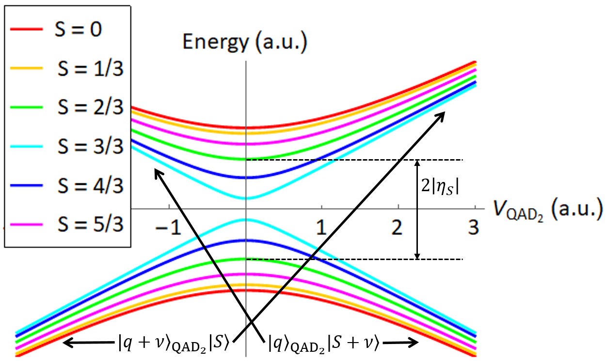
Figure 2: Energy of adiabatic states when injecting a quasiparticle from $\mathrm{QAD}_{2}$. The states of different $S$ have different energies and hence accumulate different dynamical phase during the process. The sensitivity of the dynamical phase to the process parameters is the origin of universal noise in our protocol.

We are now in a position to discuss the pumping protocol whose cycle is schematically shown in Fig. 1c. After the sequence of injection attempts from $\mathrm{QAD}_{1}$, the system evolves into a state with $Q=Q_{\mathrm{B}}$, say, $|m_{1},Q_{B},m_{3}\rangle$. The injection of a QP from $\mathrm{QAD}_{2}$ evolves this state to

$$\sum_{S=0}^{2-\nu}e^{i\theta_{S}}|m_{1},S+\nu,m_{3}+1\rangle\langle m_{1},S,m_{3}|m_{1},Q_{\mathrm{B}},m_{3}\rangle\\ =\sum_{Q}A_{Q}|m_{1},Q,m_{3}+1\rangle,$$ (17)

$$A_{Q}=\frac{1}{d}\sum_{S=0}^{2-\nu}e^{i\pi d(Q-Q_{\mathrm{B}})S/2+i\pi Q+i\theta_{S}}.$$ (18)

Therefore, the probability of pumping $r$ QPs from $\mathrm{QAD}_{1}$ in the next pumping cycle is given by $\left|A_{Q=Q_{\mathrm{B}}-r\nu}\right|^{2}$.

Assume that in each pumping cycle the limiting $\mathrm{QAD}_{2}$ potential $V_{0}$ is slightly different. The phases $\theta_{S}$ exhibit then cycle-to-cycle fluctuations; we are interested in the probabilities $\left|A_{Q=Q_{\mathrm{B}}-r\nu}\right|^{2}$ averaged over these fluctuations:

$$\langle\left|A_{Q}\right|^{2}\rangle_{\delta V_{0}}=\frac{1}{d^{2}}\sum_{S,S^{\prime}=0}^{2-\nu}e^{i\pi d(Q-Q_{\mathrm{B}})(S-S^{\prime})/2}\langle e^{i(\theta_{S}-\theta_{S^{\prime}})}\rangle_{\delta V_{0}}.$$ (19)

Note that

$$\delta\theta_{S}-\delta\theta_{S^{\prime}}=2\frac{|\eta_{S}|^{2}-|\eta_{S^{\prime}}|^{2}}{\lambda}\frac{\delta V_{0}}{V_{0}}$$ (20)

diverges in the adiabatic limit for arbitrarily small fluctuations $\delta V_{0}$, provided that $|\eta_{S}|\neq|\eta_{S^{\prime}}|$; the latter is generically true. Hence, $\langle e^{i(\theta_{S}-\theta_{S^{\prime}})}\rangle_{\delta V_{0}}=0$ for $S\neq S^{\prime}$ and $\langle\left|A_{Q}\right|^{2}\rangle_{\delta V_{0}}=1/d$. Therefore, the number of QPs pumped from $\mathrm{QAD}_{1}$ in each cycle has a universal probability distribution, leading to a universal counting statistics of the pumping current. In particular, the average current and the zero-frequency noise are given by Eq. (1).

Discussion.—The topological nature of our parafermion system gives rise to a degenerate set of “scattering states”. The latter render charge pumping in the adiabatic limit noisy. In sharp contrast to earlier studies of noisy pumping, here the average current as well as the noise (and, in fact, the entire counting statistics) are found to be topology-related universal. Specifically, the Fano factor $(d+1)e^{*}/6$ is directly related to the topological degeneracy $d$ of the parafermionic space. In analogy with the quantum Hall effect, where static disorder is needed to provide robustness to the quantized Hall conductance, here we require (minute) time-dependent (cycle-to-cycle) variations of the pumping parameters used for $\mathrm{QAD}_{2}$. Majorana zero modes are a special case of our protocol ($d=2$). In that case, the system does not support fractional quasiparticles, and one pumps electrons (rather than fractionally charged anyons) into the array of topological modes; therefore, conventional quantum dots (rather than quantum antidots embedded in FQH puddles) can be employed. For realizing the Majorana array, one can use the boundary between two $\nu=1$ quantum Hall puddles or, alternatively, a set of Majorana wires. The Fano factor will then be $1/2$.