Spin-specific heat determination of the ratio of competing first- and second-neighbor exchange interactions in frustrated spin-$\frac{1}{2}$ chains

Abstract

The magnetic susceptibility $\chi(T)$ of spin-1/2 chains is widely used to quantify exchange interactions, even though $\chi(T)$ is similar for different combinations of ferromagnetic $J_{1}$ between first neighbors and antiferromagnetic $J_{2}$ between second neighbors. We point out that the spin specific heat $C(T)$ directly determines the ratio $\alpha=J_{2}/|J_{1}|$ of competing interactions. The $J_{1}-J_{2}$ model is used to fit the isothermal magnetization $M(T,H)$ and $C(T,H)$ of spin-1/2 Cu(II) chains in LiCuSbO₄. By fixing $\alpha$, $C(T)$ resolves the offsetting $J_{1}$, $\alpha$ combinations obtained from $M(T,H)$ in cuprates with frustrated spin chains.

I Introduction

Spin-1/2 chains with isotropic exchange $J_{1}$, $J_{2}$ between first and second neighbors have been extensively studied both theoretically and experimentally. Theoretical interest has focused on the exotic quantum phases of many-spin systems with frustrated interactions and variable magnetization in an applied field Sudan et al. (2009); Furukawa et al. (2012); Sirker et al. (2011). The ground states are analyzed using field theory, density matrix renormalization group (DMRG) calculations White (1992); *white-prb93; Schollwöck (2005) and Monte Carlo simulations Sandvik (2010). Crystals that contain edge sharing chains of spin-1/2 Cu(II) sites with two bridging oxygen ligands are experimental realizations with ferromagnetic ($J_{1}<0$) first neighbor and antiferromagnetic ($J_{2}>0$) second neighbor exchange Hase et al. (2004). We refer later to specific cuprates.

The thermodynamics of spin chains, frustrated or not, are obtained by exact diagonalization (ED), as pioneered by Bonner and Fisher Bonner and Fisher (1964), or more recently by transfer matrix renormalization group (TMRG) calculations Lu et al. (2006); Sirker (2010); Xiang (1998). Isotropic exchange is the starting point for detailed magnetic characterization, as recognized in linear Heisenberg chains with $J_{1}$ of either sign. Many kinds of extended linear chain compounds are collected in Ref. *[][andreferencestherein.]miller83. Exchange-coupled chains describe materials with otherwise different spin Hamiltonians, and exotic phases or field-induced quantum transitions are typically discussed in models with isotropic exchange.

The $J_{1}-J_{2}$ model (Eq. 2 below) with $J_{1}<0$ and $J_{2}>0$ has an exact quantum critical point Hamada et al. (1988) at $\alpha_{c}=J_{2}/|J_{1}|=1/4$. The ferromagnetic ground state for $\alpha<\alpha_{c}$ switches to a singlet ($S=0$) for larger $\alpha$ The linear Heisenberg antiferromagnet (HAF) has $J_{1}>0$ and $\alpha=0$ in Eq. 2. Alternatively, it is the $\alpha\to\infty$ limit when Eq. 2 describes decoupled HAFs on sublattices of odd and even-numbered sites. The many exact HAF results Johnston et al. (2000) serve as reference for spin chains in general.

We model in this paper the thermodynamics Dutton et al. (2012) of the $J_{1}<0$ chains in LiCuSbO₄ and show that the spin specific heat directly determines the ratio $\alpha=J_{2}/|J_{1}|$. The relevant quantities are the magnetization $M(T,H)$ and the spin specific heat $C(T,P)$ at temperature $T$ and applied magnetic field $H$. In principle, the $T$ and $H$ dependencies of $J_{1}-J_{2}$ models are fully specified by the exchanges and a scalar $g$ factor, and HAFs illustrate such modeling.

Multiple quantum phases in frustrated systems are generated by small changes of competing interactions. The trade off between $J_{1}$ and $\alpha$ has already been noted in the magnetic susceptibility $\chi(T)$ of the $J_{1}-J_{2}$ model Lu et al. (2006); Sirker (2010). More negative $J_{1}$ in the singlet phase can be offset by larger $\alpha>1/4$. By contrast, the spin specific heat $C(T)$ is sensitive to $J_{1}<0$ and $\alpha$. The model with $\alpha_{c}<\alpha<0.40$ has a sharp $C(T)$ peak at low temperature followed by a broad maximum, while larger $\alpha$ leads to a single peak Heidrich-Meisner et al. (2006); Sirker (2010). What has not been appreciated is that $C(T_{m})$ at the peak directly specifies $\alpha$

$$C(T_{m})=Rf(\alpha),\qquad R=k_{B}N_{A}.$$ (1)

$R$ is the gas constant. The specific heat is the ideal thermodynamic property for quantifying the competition between $J_{1}<0$ and $J_{2}$. It has unfortunately not been reported in otherwise well studied frustrated spin chains that are mentioned in the Discussion. We propose that the specific heat should be routinely included when modeling such systems.

An overall modeling of $M(T,H)$ and $C(T,H)$ data with a few parameters is challenging and decisive but elementary. It is complementary to the ground state properties such as the magnetization $M(0,H)$, exotic quantum phases, energy gaps in incommensurate phases or spin correlation functions that are obtained by advanced methods.

II Spin specific heat and magnetization

We apply standard thermodynamics to the exact energy spectrum of finite systems with $2^{N}$ spin states, just over $1.6\times 10^{7}$ for $N=24$. The $J_{1}-J_{2}$ model with $|J_{1}|=1$ and $S_{r}=1/2$ at Cu site $r$ is

$$H(\alpha,h)=-\sum_{r}\vec{S}_{r}\cdot\vec{S}_{r+1}+\alpha\sum_{r}\vec{S}_{r}\cdot\vec{S}_{r+2}-h\sum_{r}S_{r}^{z}.$$ (2)

The interaction with the field is $h=g\mu_{B}H/|J_{1}|$ where $\mu_{B}$ is the Bohr magneton. We solve at $h=0$ for $N$ spins and periodic boundary conditions. Let $E_{jS}$ be the $j^{\text{th}}$ state in the sector with total spin $S\leq N/2$. The Zeeman levels are $-hm_{jS}$ with $m_{jS}$ running from $-S$ to $S$. The partition function with $\beta=1/k_{B}T$ of a system of $N$ spins is

$$Q_{N}(T,H)=\sum_{S=0}^{N/2}\sum_{j=1}\sum_{m_{jS}=-S}^{S}\exp\left(-\beta(E_{jS}-hm_{jS})\right).$$ (3)

The internal energy is $\langle E_{N}(T,H)\rangle=-\partial\ln Q_{N}(T,H)/\partial\beta$. The molar specific heat is

$$C_{N}(T,H)/R=\left(\beta J_{1}\right)^{2}\left(\langle E_{N}(T,H)^{2}\rangle-\langle E_{N}(T,H)\rangle^{2}\right)/N.$$ (4)

The molar magnetization is

$$M(T,H)=g\mu_{B}\frac{N_{A}}{N}\frac{\partial\ln Q_{N}(T,H)}{\partial\left(\beta h\right)}.$$ (5)

The molar susceptibility is $\chi(T)=(\partial M(T,H)/\partial H)_{0}$. We take the reported $g=2.18$ based on electron spin resonance Grafe et al. (2017) of polycrystalline LiCuSbO₄ and neglect the small, temperature independent diamagnetism or van Vleck paramagnetism. $M(T,H)$ is then entirely due to $H(\alpha,h)$.

The synthesis, structure and thermomagnetic properties of LiCuSbO₄ are published in Ref Dutton et al., 2012. $M(T,H)$ and $C(T,H)$ data were collected down to $T=2$ K and 0.1 K, respectively, and up to $\mu_{0}H=16$ T. Representative magnetic data, inelastic neutron scattering and limited modeling indicated that LiCuSbO₄ is a frustrated spin-1/2 chain Dutton et al. (2012). Here we analyze additional isothermal measurements that were collected at the same time as the published results on the same sample using the same 16 T CRYOGENIC Cryogen Free Measurement System (CFMS). The present goal is to model quantitatively the entire $M(T,H)$ and $C(T,H)$ data set at $T>5$ K, below which finite-size effects become important.

Figure 1, upper panel, shows $\chi(T)$ curves for different parameters that return equal $\chi(T^{*})$ at the peak. The inset expands the region of the $\chi(T)$ peak. Calculations for 20 spins with these parameters suffer from finite-size effects below about 5 K, as demonstrated by comparison with $N=16$ and 24 results. The size dependence is negligible at or above the $\chi(T)$ peak. Accurate data and careful analysis are needed to extract parameters from $\chi(T)$, which is often the first reported measurement on prospective spin chains. Reasonable fits are far from unique.

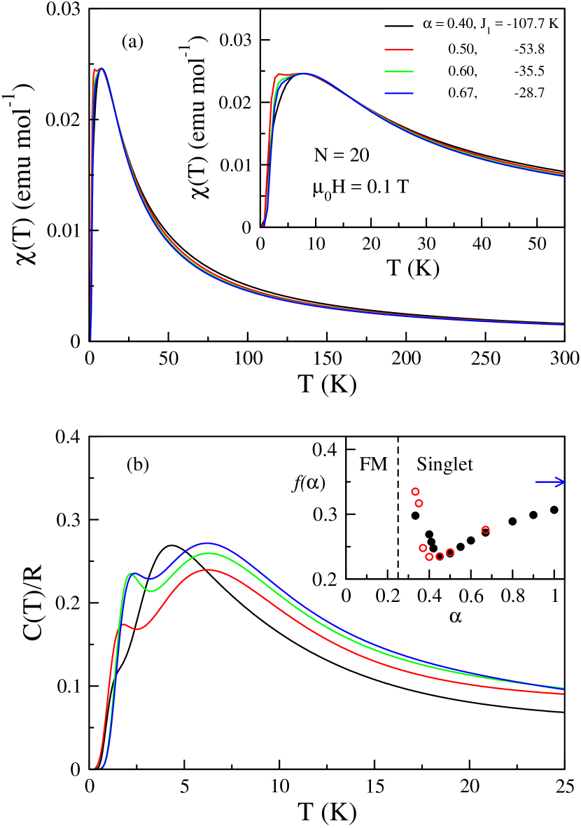
Figure 1: (a) Magnetic susceptibility $\chi(T)$ of $J_{1}-J_{2}$ models with 20 spins and $\alpha$, $J_{1}$ chosen to have equal $\chi(T^{*})$ at the peak. (b) Molar specific heat $C(T)/R$ for the same parameters. The inset shows the peak $C(T_{m})/R=f(\alpha)$ in the singlet phase; filled points refer to 20 spins calculations, open point to 24 spins, and the arrow to the limit $\alpha\to\infty$.

The zero-field specific heat $C(T)$ in Fig. 1, lower panel, is far more sensitive to the same parameters. In contrast to $\chi(T)$, there is no trade off: Scaling both exchanges scales the peak temperature $T_{m}$ without changing $C(T_{m})$. The inset to the lower panel shows $f(\alpha)$ from $\alpha>\alpha_{c}=1/4$, where it diverges, to $\alpha=1$. Open and closed circles are exact calculations with $N=24$ and 20 spins, respectively. The open circle at $\alpha=1/3$ was reported by Heidrich-Meisner et al. Heidrich-Meisner et al. (2006) who discussed the numerical challenges and used translational symmetry. We also work in k-space with periodic boundary conditions in sectors with total $S^{z}\leq N/2$. The arrow marks $f=0.3497121$ for the HAF Johnston et al. (2000), the $\alpha\to\infty$ limit. The calculated and measured molar specific heat, $C_{p}\equiv C_{v}$, of the $J_{1}-J_{2}$ model with $J_{1}<0$ restricts $\alpha$ to at most two values. Fixing $\alpha$ leaves a single exchange, just as in HAFs where magnetic data routinely yield the exchange to an accuracy of a few percent.

The message of Fig. 1 is to start with $C(T,H)$. The zero-field peak $C(T_{m})$ fixes $\alpha$ of the $J_{1}-J_{2}$ model. We then chose $J_{1}$ to fit the susceptibility peak $\chi(T^{*})$. Other $M(T,H)$ data could be used since the goal is to model all thermodynamics with $J_{1}$ and $\alpha$.

The measured specific heat is the sum of the spin part, Eq. 4, and a lattice contribution, $C_{L}(T)=aT^{3}+bT^{5}$. The first term is the Debye result. Blackman Blackman (1941) showed that $T^{5}$ corrections may appear as low as $\Theta_{D}/50$ where $\Theta_{D}\sim 200K$ is the Debye temperature. Since $C_{L}(T)$ is not known separately, we chose a procedure that assumes an $H$-independent lattice specific heat. The apparent lattice contribution is the difference between the measured specific heat and the calculated spin contribution

$$C_{\text{app}}(T,H)=C_{\text{expt}}(T,H)-C_{\text{calc}}(T,H).$$ (6)

Perfect agreement with a spin chain collapses the data at all fields to $C_{L}(T)=aT^{3}+bT^{5}$. Deviations from $C_{L}(T)$ indicate approximate modeling of the spin specific heat.

Figure 2, top panel, shows the experimental $C(T,H)$ of LiCuSbO₄ at $\mu_{0}H=0$, 4, 9 and 12 T. The field dependence is strong. The calculated lines are for 20 spins with $\alpha=0.67$, $J_{1}=-28.7$ K in Eq. 2 and $C_{L}(T)$ obtained from Eq. 6. The lower panel has $N=20$ results at these and other fields. Finite size effects appear as expected below 5 K. The apparent lattice contribution at higher temperature is almost field independent and follows the Debye law.

Figure 2: (a) Molar specific heat $C(T,H)$ of LiCuSbO₄ at $\mu_{0}H=0$, 4, 9 and 12 T. The calculated lines are for $N=20$ spins in Eq. 2 with $\alpha=0.67$, $J_{1}=-28.7$ K. (b) The lattice contribution is $C_{L}(T)=aT^{3}+bT^{5}$ obtained from Eq. 6 at the indicated fields $H$.

Grafe et al. Grafe et al. (2017) recently discussed LiCuSbO₄ by generalizing the $J_{1}-J_{2}$ model, Eq. 2, to have alternating exchanges $J_{1}(1\pm\delta)$ along the chain. This is possible in principle since there are two Cu atoms per unit cell along the chain and exchange interactions depend sensitively on bond lengths and angles Hatfield et al. (1983). LiCuSbO₄ has chains with equal Cu-Cu separations but slightly different Cu-O bond lengths and Cu-O-Cu angles Dutton et al. (2012). At constant $\alpha$, dimerization $\delta$ increases $C(T_{m})$. The $C(T,H)$ data in Fig. 2 are almost as well fit with $\alpha=0.55$, $\delta=0.15$ and $J_{1}=-41.1$ K. The additional flexibility does improve agreement with experiment in this case. We did not search for ($\alpha$, $\delta$) combinations with smaller $\delta$. The thermodynamics modeled down to 5 K are compatible with finite $\delta$. On the other hand, the spin specific heat was overlooked and is clearly incompatible with Grafe et al. (2017) $\alpha=0.28$. We expect that direct evaluation of $\alpha$ via $C(T_{m})$ will improve the exchange estimates in related cuprates with frustrated spin-1/2 chains.

Figure 3, upper panel, compares the experimental $\chi(T)$ with the almost identical calculated susceptibility for $\delta=0$, $\alpha=0.67$ and $\delta=0.15$, $\alpha=0.55$. The lower panel shows the same comparisons for $M(T,H)/H$ at $\mu_{0}H=8$ and 16 T with solid and dashed lines for $\delta=0$ and 0.15, respectively. We see again that different parameters return very similar magnetic data but distinguishable specific heat. The agreement is good but not perfect. The magnetic moment of fully aligned spins is $M=N_{A}g\mu_{B}/2$ and gives the $M/H=0.038$ intercept at 16 T. We note that Eq. 2 has to be modified in high fields to tensor rather than scalar $g$ and to include deviations from isotropic exchange. We found comparably accurate fits for $J_{1}-J_{2}$ models with $\alpha$ between 0.40 to 0.67 and offsetting $J_{1}$ chosen as in Fig. 1 to fix $\chi(T^{*})$ at the peak. Dimerized models with $\delta\sim 0.25$ and $0.4<\alpha<0.5$ also fit the magnetism and return improved $C(T,H)$ that, however, are less satisfactory than shown in Fig. 2.

Figure 3: (a) Magnetic susceptibility $\chi(T)$ of LiCuSbO₄. The calculated lines are for 20 spins in Eq. 2 with (solid line) $\alpha=0.67$, $J_{1}=-28.7$ K and (dashed line) $\alpha=0.55$, $\delta=0.15$, $J_{1}=-41.1$ K; $J_{1}$ is chosen to fit the peak $\chi(T^{*})$. (b) $M(T,H)/H$ vs. $T$ at $\mu_{0}H=8$ and 16 T for the same model parameters.

Figure 4 shows the field dependence of $M(T,H)/H$ at the indicated temperatures. Good fits are obtained at low $H$ or high $T$. DMRG yields the ground state magnetization $M(0,H)$ for $N>100$ spins Parvej and Kumar (2017). Models with isotropic exchange and scalar $g$ have a sharp field-induced transition at 0 K to the ferromagnetic state with fully aligned spins. The absolute ground state above the saturation field $H_{s}$ is the Zeeman level $S^{z}=S=N/2$. The calculated $\mu_{0}H_{s}$ are respectively 12.5 and 12.3 T for the $\delta=0$ and 0.15 fits. Quite generally, we find $\mu_{0}H_{s}\sim 12$ T for parameters based on $\chi(T)$. The measured $dM(T,H)/dH$ at $T=2$ K shows Dutton et al. (2012) a peak centered around 12 T with width of 2 T. More realistically, a $g$-tensor yields a range of saturation fields in systems with isotropic exchange. Moreover, deviations from isotropic exchange smear out $H_{s}$ because the total spin is then not conserved.

Figure 4: $M(T,H)/H$ vs. $\mu_{0}H$ of LiCuSbO₄ at the indicated temperatures. The calculated blue and red lines are for 20 spins in Eq. 2 with $\alpha=0.67$, $J_{1}=-28.7$ K and $\alpha=0.55$, $\delta=0.15$, $J_{1}=-41.1$ K.

III Discussion

All $C(T,H)$ and $M(T,H)$ data for LiCuSbO₄ have been analyzed with two parameters ($J_{1}$, $\alpha$) in $J_{1}-J_{2}$ models or three parameters ($J_{1}$, $\alpha$, $\delta$) in dimerized cases. The field dependence has scalar $g=2.18$ taken from experiment Grafe et al. (2017). The thermodynamics are governed by $H(\alpha,h)$, Eq. 2, even though the Hamiltonian is known to be approximate and incomplete. It is approximate because spin-orbit coupling generates $g$ tensors and deviations from isotropic exchange. It is incomplete because the full Hamiltonian has dipole-dipole interactions between spins, hyperfine interactions with nuclear spins and various interactions between spins in different chains.

The function $f(\alpha)$ in Eq. 1 and the inset of Fig. 1(b) directly relates the measured maximum $C(T_{m})$ of the zero-field specific heat to the ratio $\alpha=J_{2}/|J_{1}|$. Once $\alpha$ is specified, $J_{1}$ is found by fitting $\chi(T)$ or other magnetic data. The competing interactions of spin-1/2 chains with $J_{1}<0$ and $J_{2}>0$ are obtained separately. The same parameters describe the quantum phases of $J_{1}-J_{2}$ models. Ground states properties provide other ways to extract $\alpha$ and $J_{1}$ using field theory or DMRG, but in our opinion none is as direct.

We turn to the accuracy of $f(\alpha)$ calculations. Since both ED and TMRG are limited to finite temperature, they fail as $\alpha\to\alpha_{c}$ where $T_{m}/|J_{1}|\to 0$. Numerical methods return accurate $f(\alpha)$ except close to $\alpha_{c}$. Finite-size effects go roughly as $|J_{1}|/N$ and are evident at $\alpha=1/3$ where $C(T_{m})/R$ increases from 0.298 to 0.334 for $N=20$ and 24, respectively. The corresponding increase at $\alpha=0.50$ and smaller $|J_{1}|$ is from 0.239 to 0.245, while $C(T_{m})$ at $\alpha=0.67$ increases by only $1.6\%$ between $N=20$ and 24. The $N=20$, $\alpha=0.67$ fits of $C(T,H)$ in Fig. 2 do not change perceptively at $N=24$ for $T\geq T_{m}$.

We conclude that $J_{1}-J_{2}$ models with $\alpha_{c}<\alpha<1/3$ have $C(T_{m})/R>0.34$. That is the range of greatest theoretical interest, close to the quantum critical point. To the best of knowledge, however, all reported $C(T_{m})/R$ indicate $\alpha>1/3$.

We turn briefly to other cuprates with $J_{1}<0$ and $J_{2}>0$. There is no indication Dutton et al. (2012) of 3-D ordering in LiCuSbO₄ down to 0.1 K, but other systems have ordering transitions at lower $T$ than the susceptibility peak. Thermodynamic data at finite $T>5$ K is not sensitive to energy differences $\Delta\epsilon\ll k_{B}T$ that for example differentiate between gapped and gapless phases of the $J_{1}-J_{2}$ model.

The measured $C(T)$ of Li₂ZrCuO₂ has Drechsler et al. (2007) $C(T_{m})/R=0.32$ and a fairly sharp peak at $T_{m}=6.4$ K that shifts to lower $T_{m}(H)$ in an applied field and is suppressed by 9 T. The $\chi(T^{*})$ maximum is 0.037 emu Oe^-1mol^-1, some $50\%$ higher than the LiCuSbO₄ peak in Fig. 3. The inferred ($\alpha$, $J_{1}$) are Drechsler et al. (2007) 0.30 and $-273$ K, with $\alpha$ emphasized to be close to $\alpha_{c}=1/4$. But $\alpha$ is at least 0.35 since $f(1/3)$ returns larger $C(T_{m})$ and $|J_{1}|$ is smaller.

The bridging ligands in linarite, PbCuSO₄(OH)₂, are OH rather than O. Single crystals make possible detailed magnetic studies Wolter et al. (2012), for example with $H$ along the principal axes of the $g$ tensor. The inferred ($\alpha$, $J_{1}$) from multiple sources are 0.36 and $-100$ K, in line with $\mu_{0}H_{s}\sim 7.6$, 8.5 and 10.5 T along the principal axes, but $C(T,H)$ has not been reported.

$M(T,H)$ measurements on Rb₂Cu₂Mo₃O₁₂ were originally analyzed Hase et al. (2004) as ($\alpha$, $J_{1}$) with $\alpha=0.37$ and $J_{1}=-138$ K. TMRG modeling of $\chi(T)$ is shown in Fig. 8 of Ref. Lu et al., 2006 for the same and related parameters without obtaining a satisfactory fit. We are not aware of $C(T,H)$ data. A $J_{1}-J_{2}$ model has also been discussed Masuda et al. (2004) for neutron diffraction and $\chi(T)$ in LiCu₂O₂. $C(T)$ was not reported and 3D ordering at $\sim 20$ K suggests going beyond a 1D model.

Banks et al. Banks et al. (2009) performed a comprehensive structural, magnetic and computational study of frustrated spin chains in CuCl₂. The crystal has Néel order below $T_{c}=23.9$ K. Contributions to the measured $C(T)/T$ are estimated Banks et al. (2009) from the lattice ($\sim 80\%$) and from overlapping peaks due to the transition and spins. The broad spin peak is at $T_{m}=35$ K where $C(T_{m})/T_{m}=0.11$ $\text{J K}^{-1}\text{mol}^{-1}$. These numbers return $f(\alpha)=0.46$ in Eq. 1, slightly higher than the HAF limit (0.35) for a $J_{1}-J_{2}$ model with $J_{1}<0$. The lattice contribution is obtained indirectly and alternative descriptions are mentioned Banks et al. (2009). So the reported $C(T_{m})$ may be consistent with $\alpha>1$ ($f>0.31$), in line with the overall antiferromagnetism.

We emphasize in closing that these cuprates are complex systems with diverse magnetic, structural, dielectric and other properties. It has been fully recognized that the $J_{1}-J_{2}$ model is merely the starting point, just as are HAFs for spin chains without frustration. In that context, however, the spin specific heat and in particular $C(T_{m})$ provide a direct evaluation of the ratio $\alpha=J_{2}/|J_{1}|$ of competing exchange interactions. We expect that $C(T,H)$ measurements will lead to more consistent ($J_{1}$, $\alpha$) parameters for cuprates with frustrated spin-1/2 chains.