Spatial Distribution of Gamma-Ray Burst Sources

1.   Introduction

According to current observational data, the sources of gamma-ray bursts (GRB) are explosions of massive supernova stars (long GRB) and mergers of neutron stars (short GRB) in distant galaxies. Thus, the spatial distribution of GRB reflects the large-scale distribution of galaxies, so that analyzing the distribution of gamma-ray bursts in space and time is an important task for the study of the evolution of the large-scale structure of the universe. The extreme luminosity of GRB makes it possible to detect their sources at large red shifts, and the available completeness of the surveys of GRB (e.g., Swift) makes it possible to use samples of GRB with known red shifts for preliminary analysis of their spatial distribution over a wide range of scales.

The standard cosmological model assumes a uniform distribution of matter in the universe, including dark matter and dark energy. Observations of the spatial distribution of visible matter (galaxies) do, however, reveal nonuniformities over scales much longer than the standard correlation length, 10 Mpc (the Sloan Great Wall, size $\sim 300$ Mpc at $z\sim 0.07$ [1,2]). In addition, the power law dependence of the conditional density of the distribution of galaxies $\Gamma(r)\propto r^{-1}$ on scales up to 100 Mpc corresponds to a fractal dimensionality $D\sim 2$ [3-5]. Large nonuniformities have recently been discovered in the distribution of galaxies in the SDSS/CMASS survey (the BOSS Great Wall, size $\sim 400$ Mpc at $z\sim 0.47$ [6]), as well as in the deep galactic survey COSMOS (Super Large Clusters with sizes $\sim 1000$ Mpc at $z\sim 1$ [7-9]).

The spatial distribution of gamma-ray bursts has been analyzed in a number of papers [10-13]. Thus, the distribution of 244 GRB has been analyzed [10] as part of the Swift mission using the $\xi$-function method. The correlation length was $r_{0}\approx 388$ h^-1 Mpc, $\gamma=1.57\pm 0.65$(at the $1\sigma$ level), and the uniformity scale was $r\geq 7700$ h^-1. Other approaches to the study of the correlation properties of the spatial structures are the conditional density method [3,4] and the pairwise distance method [14]. In Ref. 11 it was applied for the first time to 201 GRB with known (at that time) angular coordinates and red shift. An estimate of $D\cong 2.2\div 2.5$ was obtained for the fractal dimensionality. This method also makes it possible to detect close pairs and triplets of points. Thus, for example, a spatially isolated group of five GRB was detected with coordinates $23^{h}$ $50^{m}<\alpha<0^{h}$ $50^{m}$ and $5^{\circ}<\beta<25^{\circ}$ a redshift of $0.81<z<0.97$. If GRB events are regarded as indicators of the presence of matter in space, then this group is indirect evidence of a supercluster of galaxies within this range of coordinates.

A giant ring of GRB with a diameter of 1720 Mpc at red shifts of $0.78<z<0.86$ has been discovered [12].The probability that this structure was found randomly is $2\times 10^{-6}$. 352 GRB have been found [13] to have an estimated dimensionality in terms of the $\Lambda CDM$ model of $D\approx 2.3\pm 0.1$. In other models, $D\approx 2.5$. The latest numerical predictions in terms of the $\Lambda CDM$ model show [15] that at large red shifts it is already possible to observe clusterization of matter, so the detection of structures in the distribution of GRB is an important problem.

In this paper, we estimate fractal dimensionality using the conditional density method for GRB for the first time and compare this estimate with estimates derived from the pairwise distance method. As a comparison with the GRB catalog, artificial fractal and uniform catalogs are modeled. Effects owing to the sample geometry are taken into account, in particular: limits on the maximum radius sphere and cutoff of the galactic belt. The evolution of luminosity with increasing red shift is examined. For the first time these plots are compared with a uniform distribution, so it is possible to compare the efficiency of the two methods. The power law dependence over a large range of scales also shows up more clearly.

2.   The sample

The Swift Gamma-ray Burst Mission on line catalog [16], which has been extended in Ref. 17 and in another on line catalog [18], is used as the basis for the GRB catalog. Our catalog of GRB sources with known red shifts contains a total of 384 objects. Our approach makes it possible to use all the points to determine the fractal dimensionality without additional truncations and selection. The only condition for including objects in the combined catalog is the existence of angular coordinates and red shifts. Thus, of the working sample ($<8$ Gpc), 377 GRB remain, for 360 of which the luminosities have been determined. The combined catalog has been updated to June 2017.

The first rows of our working sample are shown in Figs. 1 and 2. The headings of the tables correspond to:the name of the event, galactic coordinates, the estimated time of the event, the received radiation in $10^{-7}$ erg/cm^-2 in the $15\div 150$ keV band during the time $T_{90}$ of the event, the red shift, the mission (Swift), metric coordinates, distance to the GRB source, the logarithm of the flux, and the logarithm of the luminosity.

3.   Methods

All the model calculations were done using the original Fractal Dimension Estimator program, which is described elsewhere.

Table 1: Original Rows of the Catalog.

name	$l$	$b$	$T_{90}$	$F_{obs}$	$z$
151215A	177.25358	8.55309	17.80	3.10	2.590
150423A	9.70821	59.24722	0.22	0.63	1.394
141121A	200.39117	26.85321	549.90	53.00	1.470
…

Table 2: Calculated Rows of the Catalog.

$X_{Mpc}$	$Y_{Mpc}$	$Z_{Mpc}$	$R_{Mpc}$	$lgS_{obs}$	$lgL_{b}$
–5862.4	281.2	882.7	5935.1	–0.75	51.97
2099.7	359.2	3580.2	4166.0	0.45	52.53
–3605.5	–1340.3	1947.5	4311.5	–1.01	51.11
…

3.1.   Conditional density

This method, which is discussed in detail in Refs. 3 and 4, essentially involves counting the number of points in spheres of different radii. The conditionality is that the center of a sphere is a point in the set. For correct operation of this method at large scales, it is necessary to take the effect of the boundary of the set into account [19]. The concentration inside a sphere of radius $r$ is given by

$$n(r)=\frac{1}{N_{c}(r)}\sum_{i=1}^{N_{c}(r)}\frac{N_{i}(r)}{V(r)},$$ (1)

where $N_{c}(r)$ is the number of spheres inside the sample, $N_{i}(r)$ is the number of points in a sphere, and $V(r)$ is the volume of a sphere. On intermediate scales this distribution has a $D-3$ power law dependence,

$$\Gamma^{*}(r)=\langle n(r^{\prime}<r)\rangle_{p}$$ (2)

where $\langle...\rangle_{p}$ denotes averaging over all points in the sample.

3.2.    Pairwise distances

The distribution of pairwise distances for sets with integral dimensionality is discussed in Ref. 20.

$$f(l)=Dl^{D-1}(L/2)^{-D}I_{\mu}(\frac{D+1}{2},\frac{1}{2}),$$ (3)

where $D$ is the integral dimensionality of the set, $l$ is the distance between a pair of points, $L$ is the greatest distance within the set, and $I_{\mu}(p,q)$ is the incomplete Bessel function with $\mu=1-l^{2}/L^{2}$. For $l<<L$ there is an asymptote

$$f(l)\sim l^{D-1},$$ (4)

which also is retained for sets with a fractional dimensionality [21,22,14].

Figure 1: Integrated distributions of the GRB with respect to distance ($\Delta R=200Mpc$) and red shift ($\Delta z=0.2$).

Figure 2: Differential distributions of the GRB with respect to distance ($\Delta R=200Mpc$) and red shift ($\Delta z=0.2$).

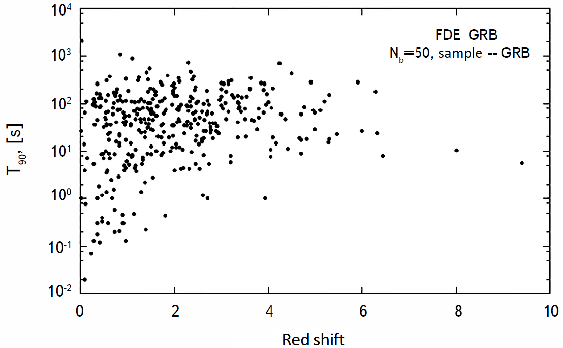
Figure 3: The distribution of $T_{90}$ with respect to red shift $z$ for all the GRB sources

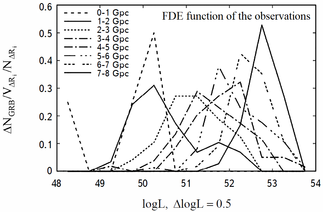
Figure 4: Observed luminosity distributions of the GRB sources in fixed distance intervals.

3.3.   Comparison of the methods

For a convenient comparison of the results of the pairwise distances and conditional density methods, plots of the ratio of the curves for a fractal or GRB to a uniform sample are ultimately examined. In this configuration the slope of the working segment, which is determined by the condition of least squares for the deviations, is equal to $D-3$ for each of the methods in logarithmic coordinates.

For sparse sets with $N<10^{3}$ the distributions of the conditional density and pairwise distances are characterized by substantial random deviations from a power law dependence. To reduce the influence of this effect, the curves are averaged over a sufficient number of runs for the given set. This is done by specifying different zero points for the pseudorandom number generator. This operation is carried out for the conditional density distributions, as well as for the pairwise distance distributions.

3.4.   Calculating the distance and luminosity

In the standard cosmological model the metric distances are given in terms of red shift by the formula [4]

$$R(z)_{Mpc}=\frac{c}{H_{0}}\int_{0}^{z}(\Omega^{0}_{v}+\Omega_{m}^{0}(1+z^{\prime})^{3}-\Omega_{k}^{0}(1+z^{\prime})^{2})^{-1/2}dz^{\prime},$$ (5)

where $H_{0}=70$ km/s/Mpc is the Hubble constant, $c=3\cdot 10^{10}$ cm/s is the speed of light, $\Omega^{0}_{v}=0.7$, $\Omega_{m}^{0}=0.3$, and $\Omega_{k}^{0}=0$ are the cosmological parameters, and $z$ is the red shift. Then the spherical coordinates are transformed to Cartesian, since the space is Euclidean. The luminosity in terms of the $\Lambda CDM$ model is given by

$$L(z)=4\pi S_{obs}R(z)_{sm}^{2}(1+z)^{2},$$ (6)

where $S_{obs}$ erg/s/cm² is the GRB flux, which equals the ratio of the radiation received in the $15\div 150$ keV range to the time $T_{90}$, and $z$ is the red shift.

3.5.   The model catalogs

Fractal and uniform sets analogous to the GRB catalog were modeled for comparison with the actual sample. Since strong absorption of visible radiation (leading to additional selection of GRB when measuring their red shift) occurs near the galactic belt, it is necessary examine the influence of this effect on the estimated fractal dimensionality. Thus, two cases were examined. Examples of these are shown in Fig. 6. The first covers the entire celestial sphere, while the band from $-10$ to $+10$ degrees of galactic latitude is cut out in the second. All of these samples are bounded by a sphere of radius 8 Gpc.

Figure 5: Distribution of the luminosities of the GRB catalog and the uniform model catalog with respect to distance.

To determine the fractal dimensionality over the entire volume right away, it is necessary to account for the observed selection effects, e.g., the Malmquist effect, for all the points. For this, the observed profiles in spherical layers with a step size of 1 Gpc shown in Fig. 4 are taken as the model visible luminosity function. Since introducing a model selectivity with respect to luminosity affects the conditional density distribution, the ratio of the curves for fractals and GRB to the uniform curves is examined.

4.   Results

4.1.   General properties of the GRB source catalog

The radial distributions of the GRB catalog are shown in Fig. 1 (integrated distributions) and Fig. 2 (differential distributions). The distribution of the time an event is observed, $T_{90}$, with respect to red shift is shown in Fig. 3. At present, the drift with increasing red shift toward shorter event times predicted by the standard model has not yet been observed. Our result is consistent with Ref. 23. A definitive answer to this question would require a significant increase in the number of GRB at large red shifts and it would be necessary to study the dependence of $T_{90}$ on the distance to the GRB source.

GRB can serve as an indicator of galactic clusters, so it is possible look for close pairs in the spatial distribution of GRB in Table 3. Of the 18 pairs, it is possible to identify spatially distinctive structures of three and four gamma-ray bursts, as well as two pairs for which the distance between the sources is less than 100 Mpc at $z\approx 0.013$ and $z\approx 1.43$.

Table 3: GRB Sources with Pairwise Distances to 300 Mpc.

N	Designation	$d_{Mpc}$	$l$	$b$	$z$
175	111005A	79.4	338.33759	34.63886	0.013
4	100316D		266.91664	–19.78007	0.014
175	111005A	195.6	338.33759	34.63886	0.013
158	060218A		166.86303	–32.86884	0.033
4	100316D	150.1	266.91664	–19.78007	0.014
158	060218A		166.86303	–32.86884	0.033
158	060218A	293.1	166.86303	–32.86884	0.033
94	051109B		100.54662	–19.39992	0.080
234	060505A	264.9	22.09128	–53.71345	0.089
54	060614A		344.08607	–43.94594	0.130
32	061201A	206.0	315.71506	–38.23391	0.111
54	060614A		344.08607	–43.94594	0.130
117	130427A	261.1	206.48629	72.51440	0.340
18	130603B		236.47527	68.43758	0.356
13	110328A	299.3	86.71625	39.42626	0.354
84	151027A		90.49260	28.48382	0.380
25	140903A	276.7	44.40465	50.11996	0.351
89	101213A		37.17510	45.89511	0.414
27	070724A	282.8	184.32601	–73.81347	0.457
315	091127A		197.38677	–66.73665	0.490
22	141212A	242.7	155.24497	–38.01808	0.596
304	130215A		163.06996	–39.75075	0.597
104	150323A	189.0	174.83011	36.29286	0.593
168	110106B		172.91003	40.47816	0.618
291	080916A	236.0	333.57758	–50.49415	0.689
124	150821A		329.53474	–52.37413	0.755
161	050824A	248.8	122.21283	–40.26635	0.830
77	080710A		116.98198	–43.17503	0.845
77	080710A	291.4	116.98198	–43.17503	0.845
271	060912A		113.49717	–41.34504	0.937
206	160131A	231.1	207.86277	–25.13766	0.970
116	120907A		208.46983	–29.19799	0.970
50	161108A	269.0	221.80332	78.92167	1.159
268	90530		212.46605	77.98286	1.266
48	050822X	77.0	255.27955	–54.45517	1.434
203	050318A		256.44382	–55.23286	1.440

4.2.   Fractal dimensionality

Figure 5 is a comparison of the luminosity distribution of the GRB with the model uniform catalog after application of the selectivity function with respect to luminosity shown in Fig. 4. Figure6 illustrates the visible differences between the real sample of GRB and the model catalogs for two geometries. In the case of the truncated celestial sphere, the sample is a superposition of two hemispheres. Plots of the conditional density and mutual distances are shown in Figs. 7 and 8, respectively. The graphs of the fractals shown here are average curves over 17 runs and this is the cause of the corresponding deviations for the points in the graphs. The amplitude of the deviations in the pairwise distance method is a factor of two larger than for the conditional density.In all runs of the fractal and uniform samples to which these methods were applied directly, the number of points is roughly equal to the number of GRB. This is done by creating an excess of points in the initial run, and then by selecting them uniformly.

Figure 6: Projections of the spatial distribution on the X-Z plane for two geometrical shapes of the sample. The top corresponds to a fractal $D=2.5$, the center to the GRB catalog, and the bottom to a uniform set.

For a more accurate result, the excess in the observed number of GRB on small radial scales must be taken into account, as discussed in Ref. 24.

Figure 7: Plots of the normalized conditional density for GRB (solid circles) and fractals $D=2.0$ (squares) and $D=2.5$ (circles) for the full celestial sphere. Unity corresponds to a uniform distribution.

Figure 8: Plots of the reduced pairwise distances for GRB (solid circles) and fractals $D=2.0$ (squares) and $D=2.5$ (circles) for the truncated celestial sphere.Unity corresponds to a uniform distribution.

5.   Conclusions

For model sets with $N>10^{3}$ points, the accuracy of the estimated fractal dimensionality reaches $\Delta D=0.06$ for the conditional density and $\Delta D=0.03$ for pairwise distances prior to introduction of the model luminosity function and prior to truncation of the galactic belt. After introducing limitations on the geometry and luminosity with the same total number of points, the accuracy of the method decreased by a factor of two. It is noteworthy that the radius of the sphere, and not the diameter, is treated as the parameter in the conditional density, so that the horizontal axis can be multiplied by a factor of two when comparing the methods. The main parameters determining the accuracy of the estimated fractal dimensionality are the number of points and the number of runs. During testing of the accuracy, it was found that the pairwise distance method is better than the conditional density method for short scales.

Thus, the pairwise distance curve reaches a power law dependence at a scale equal to twice the size of the elementary cell of the fractal structure. At the same time the conditional density begins to operate at a scale that is $4\div 8$ times the size of the elementary cell, depending on the representativeness of the sample and the value of the fractal dimensionality. On large scales both methods have problems. In the conditional density, averaging is over a small number of spheres, while in the pairwise distances the distribution behaves unpredictably or is close to uniform.

For the case of a full celestial sphere, the estimated fractal dimensionality of the distribution of the GRB sources was $D=2.6\pm 0.12$ at $R=1.5\div 2.5$ ($d=3\div 5$) Gpc for the conditional density and $D=2.6\pm 0.06$ for $l=1.5\div 5.5$ Gpc. In the case with a truncated galactic belt, the conditional density does not yield a unique result and its distribution does not differ from uniform. The pairwise distances have a stable power law dependence with $D=2.6\pm 0.06$ and essentially do not change the interval for the linear segment $l=1.5\div 5.5$. Thus, on scales of $\approx 3\div 5$ Gpc, there is a power law correlation between the methods.

At distances close to $D=3$, when selection effects are taken into account the methods yield a systematically high estimate for the model sets by roughly $\Delta D=0.1$. Given this bias, it is necessary to correct the result in order to obtain a more accurate estimate. Thus, the estimated fractal dimensionality of the observed GRB distribution is $D=2.55\pm 0.06$.

References

- [1] J. R. Gott III, M. Jurić, D. Schlegel et al., Astrophys. J. 624, 463 (2005).
- [2] M. Einasto, et al., Astron. Astrophys. 595, A70 (2016).
- [3] A. Gabrielli, F. Sylos Labini, M. Joice, and L. Pietronero, Statistical Physics for Cosmic Structures, Springer, Berlin (2005).
- [4] Yu. V. Baryshev and P. Teerikorpi, Fundamental Questions of Practical Cosmology, Astrophysics and Space Science Library, 383, Springer Science, Dordrecht (2012).
- [5] D. I. Tekhanovich and Yu. V. Baryshev, Astroph. Bull. 71, 155 (2016).
- [6] H. Lietzen, E. Tempel, L. J. Liivamägi, et al., Astron. Astrophys. 588, L4 (2016).
- [7] N. V. Nabokov and Yu. V. Baryshev, Astrophysics, 53, 101 (2010).
- [8] S. I. Shirokov, D. I. Tekhanovich, and Yu. V. Baryshev, Vestnik SPbGU 59, 659 (2014).
- [9] S. I. Shirokov, N. Yu. Lovyagin, Yu. V. Baryshev, and V. L. Gorokhov, Astron. Rep. 60, 563 (2016).
- [10] Ming-Hua Li and Hai-Nan Lin, Astron. Astrophys. 582, A111 (2015).
- [11] A. A. Raikov, V. V. Orlov, and O. B. Beketov, Astrophysics, 53, 396 (2010).
- [12] L. G. Balázs, Z. Bagoly, J. E. Hakkila, I. Horváth, J. Kóbori, I. I. Rácz, and L. V. Tóth, Mon. Not. Roy. Astron. Soc. 452, 2236 (2015).
- [13] R. V. Gerasim, V. V. Orlov, and A. A. Raikov, Astrophysics, 58, 204 (2015).
- [14] A. A. Raikov and V. V. Orlov, Mon. Not. Roy. Astron. Soc. 418, 2558 (2011).
- [15] A. K. Bhowmick, T. Di Matteo, Y. Feng, and F. Lanusse, Mon. Not. Roy. Astron. Soc. (2017).
- [16] https://swift.gsfc.nasa.gov/archive/grb_table/
- [17] J. S. Wang, F. Y. Wang, and K. S. Cheng, & Z. G. Dai, Astron. Astrophys. 585, A68 (2016).
- [18] http://www.grbcatalog.org
- [19] F. Sylos Labini, M. Montuori, and L. Pietronero, Phys. Rept. 293, 61 (1998).
- [20] M.G. Kendall and P.A.P. Moran, Geometrical Probability, Griffin, London (1963).
- [21] P. Grassberger and I. Procaccia, Phys. Rev. Lett. 50, 346 (1983).
- [22] P. Grassberger and I. Procaccia, Physica D: Nonlinear Phenom. 9, 189 (1983).
- [23] D. Kocevski and V. Petrosian, Astroph. J. 765, 116 (2013).
- [24] H. Yu, F. Y. Wang, Z. G. Dai, and K. S. Cheng, Astrophys. J. Suppl. Ser 218, 12 (2015).