Resset: A Recurrent Model for Sequence of Sets with Applications to Electronic Medical Records

Abstract

Modern healthcare is ripe for disruption by AI. A game changer would be automatic understanding the latent processes from electronic medical records, which are being collected for billions of people worldwide. However, these healthcare processes are complicated by the interaction between at least three dynamic components: the illness which involves multiple diseases, the care which involves multiple treatments, and the recording practice which is biased and erroneous. Existing methods are inadequate in capturing the dynamic structure of care. We propose Resset, an end-to-end recurrent model that reads medical record and predicts future risk. The model adopts the algebraic view in that discrete medical objects are embedded into continuous vectors lying in the same space. We formulate the problem as modeling sequences of sets, a novel setting that have rarely, if not, been addressed. Within Resset, the bag of diseases recorded at each clinic visit is modeled as function of sets. The same hold for the bag of treatments. The interaction between the disease bag and the treatment bag at a visit is modeled in several, one of which as residual of diseases minus the treatments. Finally, the health trajectory, which is a sequence of visits, is modeled using a recurrent neural network. We report results on over a hundred thousand hospital visits by patients suffered from two costly chronic diseases – diabetes and mental health. Resset shows promises in multiple predictive tasks such as readmission prediction, treatments recommendation and diseases progression.

I Introduction

After stunning successes in cognitive domains, deep learning is expected to transform healthcare [21]. Most remarkable results thus far in health have been in diagnostic imaging [7, 9], which is a natural step given record–breaking results in computer vision. However, diagnostic imaging is only a small part of the story. A full intelligent medical system should be able to reason about the past (historical illness), present (diagnosis) and future (prognosis). Here we adopt the notion of reasoning as “algebraically manipulating previously acquired knowledge in order to answer a new question” [1]. For that we learn to embed discrete medical objects into continuous vectors, which lend themselves to a wide host of powerful algebraic and statistical operators [3, 22]. For example, with diseases represented as vectors, computing disease-disease correlation is simply a cosine similarity between the two corresponding vectors. Illness – recorded as a bag of discrete diseases – can then be a function of set of vectors. The same holds for care. Importantly, if diseases, treatments (or even doctors) are embedded in the same space then recommendation of treatments (or doctors) for a given disease will be as simple as finding the nearest vectors.

The algebraic view makes it easily to adapt powerful tools from the recent deep learning advances [15] for healthcare. In particular, we can build end-to-end models for risk prediction without manual feature engineering [2, 16, 17, 19]. As the models are fully differentiable, credit assignment to distant risk factors can be carried out [16], making the models more transparent than commonly thought. The learning path through recorded medical data necessitates the modeling of the dynamic interaction between the three processes: the illness, the care and the data recording [17]. For the purpose of this paper, we assume that a clinic visit at a time manifests through a set of discrete diseases and treatments. A healthcare trajectory is therefore a sequence of time-stamped records. This necessitates a set-theoretic treatment of each visit and a dynamic treatment of the entire trajectory.

We introduce $\mathsf{\mathtt{Resset}}$, a recurrent model of healthcare trajectory as a sequence of sets. Although neural modeling of unordered sets has been recently studied [24, 26], sequences of sets have not been formally investigated, to the best of our knowledge. In $\mathsf{\mathtt{Resset}}$, features for a set are computed through a multi-valued set function, which is permutation invariant. There are two set functions, one for diseases and the other for treatments. A dual-input function of these two set functions encodes the multi-disease–multi-treatment interaction at the visit level. Finally, visits are connected through a LSTM to model the temporal dynamics between visits.

With this design, $\mathsf{\mathtt{Resset}}$ addresses an important aspect of healthcare: the dynamic interaction between illness and care. Although care is supposed to lessen the illness, it is often designed through highly controlled trials where one treatment is targeted at one disease, on a specific cohort, at a specific time [12]. Much less is known for the effect of multiple treatments on multiple diseases, in general hospitalized patients, over time. A recent model known as DeepCare [17] partly addresses this problem by considering the moderation effect of treatments on illness state transition between visits. However, unlike $\mathsf{\mathtt{Resset}}$, DeepCare does not address the multi-disease–multi-treatment interaction within visits.

We evaluate $\mathsf{\mathtt{Resset}}$ on the task of predicting the important medical outcomes such as unplanned readmission or death at discharge, treatment recommendation and future diseases. We focus on chronic diseases (diabetes and mental health) as they are highly complex with multiple causes, often associated with multiple comorbidities, and the treatments are not always effective. Results from over one hundred thousand visits to a large regional hospital data demonstrate the efficacy of $\mathsf{\mathtt{Resset}}$.

To summarize, we claim the following contributions: 1) A novel representation of time-stamped healthcare trajectory as a sequence of sets. 2) A novel deep learning architecture for sequence of sets called $\mathsf{\mathtt{Resset}}$, which – when applied to healthcare – uncovers the structure of the disease/treatment space and predicts future outcomes. 3) An evaluation of these claimed capabilities on real patients with hundred thousands of hospital visits on three tasks: readmission prediction, treatments recommendation and diseases progression.

The rest of the paper is organized as follows. Section II briefly review related work in healthcare and deep learning. Section III presents $\mathsf{\mathtt{Resset}}$ in context of healthcare trajectory modeling. Experimental results are reported in Section IV. Finally, Section V concludes the paper.

II Related Work

II-A Deep Learning for Healthcare

The past few years have witnessed an intense interest in applying recent deep learning advances to healthcare [19]. The most ready area is perhaps medical imaging [8]. Thanks to the record-breaking successes in convolutional nets in computer vision, we now can achieve diagnosis accuracy comparable with experts in certain sub-areas such as skin-cancer [7]. However, it is largely open to see if deep learning succeeds in other areas where data are less well-structured and of lower quality such as electronic medical records (EMR) [17].

Within EMRs, three set of techniques have been employed. The first is finding distributed representation of medical objects such as diseases, treatments and visits [3, 22]. The techniques are not strictly deep but they offer a compelling algebraic view of healthcare. The second group of techniques involve 1D convolutional nets, which are designed for detecting short translation invariant motifs over time [2, 16]. The third group, to which this paper belongs, employs recurrent neural nets to capture the temporal structure of care [4, 17]. For more comprehensive review of this highly dynamic research area in recent time, we refer to [20].

Predictive healthcare begs the question of modeling treatment effects over time. This has traditionally been in the realm of randomized controlled trials. Our work here is, on the other hand, based entirely on observational administrative data stored in Electronic Medical Records.

II-B Neural Nets for Sets

Sets are fundamental to mathematics, and are pervasive in many learning tasks such as clustering (set membership assignment), feature selection (subset of features), multi-label learning (subset of labels) and multi-instance learning (set classification). Due to its permutation-invariance and variation in size, set does not lend itself naturally to traditional neural networks. In [24], mapping set to set is framed as mapping sequence to sequence, in which a set is “pretended” to be a pseudo-sequence. This does not address the permutation-invariant property of sets. A more systematic investigation is [26], where conditions for set functions are specified. Sets have also been studied indirectly, e.g., in pooling operations in CNN; in attention mechanism (e.g., see [23]) – which is essentially a function over sets, in deep multi-X learning [18]. Predicting sets have also been studied in [10]. In the existing literature, neural models of sequences of sets seem to be missing.

III Methods

Figure 1: $\mathsf{\mathtt{Resset}}$ for sequence of sets, as a model of healthcare trajectory.

In this section, we present our main modeling contribution, the $\mathsf{\mathtt{Resset}}$ as a recurrent model for sequence of sets, in the context of its primary application in healthcare.

III-A Set Function

Let us start with set, an unordered collection of elements. Let $S=\left\{\boldsymbol{e}_{1},\boldsymbol{e}_{2},...\right\}$ be a set of vectors in $\mathbb{R}^{n}$. A set function $f(S)$ is a mapping invariant against permutation of set elements, that is, $f(S)=f(\pi S)$, for any permutation operator $\pi$. For simplicity, we are interested in a function $f(S)$ that receives a set of vectors $S$ and returns another vector in the same real space $\mathbb{R}^{n}$. We use the following normalized set function:

$$f(S) \leftarrow\frac{\bar{\boldsymbol{e}}_{S}}{\epsilon+\left\|\bar{\boldsymbol{e}}_{S}\right\|}\quad\text{where}\quad\bar{\boldsymbol{e}}_{S}=\max\left(\mathbf{0},\sum_{i\in S}\boldsymbol{e}_{i}\right)$$ (1)

where $\epsilon>0$ is a smoothing factor. This is essentially a linear rectifier of the sum, approximately normalized to unit vector. The factor $\epsilon$ lets $\left\|f(S)\right\|\rightarrow 0$ when$\left\|\bar{\boldsymbol{e}}_{S}\right\|\rightarrow 0$, but $\left\|f(S)\right\|\rightarrow 1$ when $\left\|\bar{\boldsymbol{e}}_{S}\right\|\gg 0$.

III-B Clinic Visit as Set-Set Interaction

Each medical record contains information about the history of clinic visits by a patient. For simplicity, we consider a visit record as a bag of diseases deemed relevant for care at the time of visit, and a bag of treatments administered for the patient. Among older cohorts, non-singleton bags are prevalent, reflecting the comorbidity picture of modern healthcare, that is, an elderly typically suffers from multiple co-occurring conditions. As a result, treatments must be carefully administered to work with, or at least not to cancel out, each other. This also calls for a sensible way to model the complexity of multi-disease–multi-treatment interaction. Most existing bio-statistics methods, however, are designed for simplified treatment effect against just one condition in a controlled experimental setting, and thus inadequate in this operational setting. Our solution is based on set-set interaction, which we detail subsequently.

We first use vector representation of diseases and treatments, following the recent practice in NLP (e.g., see [5]). Let $\boldsymbol{e}_{d}$ be the embedding of disease $d$, $\boldsymbol{e}_{p}$ the representation of the treatment $p$, and the vectors are embedded in a common space. The bags of diseases and bags of treatments are also represented as vectors in the same space.

Denote by $D_{t}$ the bag of diseases and $I_{t}$ the bag of treatments recorded for the visit at time $t$. Let $\boldsymbol{d}_{t}=f\left(D_{t}\right)$ be the set representation of the disease bag, and $\boldsymbol{p}_{t}=f\left(I_{t}\right)$ the set representation of the treatment bag, as given in Eq. (1). Let $\boldsymbol{v}_{t}=g\left(\boldsymbol{d}_{t},\boldsymbol{p}_{t}\right)$ denote the interaction function between diseases, as encapsulated in $\boldsymbol{d}_{t}$, and treatments, as coded in $\boldsymbol{p}_{t}$. A popular method is to use a bilinear function, e.g., $\boldsymbol{v}_{t}^{k}=\rho\left(\boldsymbol{d}_{t}^{\top}W^{k}\boldsymbol{p}_{t}\right)$ where $W^{k}$ is a matrix and $\rho$ is an element-wise nonlinear transformation, but this will result in lots of parameters.

One intuitive function is as follows:

$$g\left(\boldsymbol{d}_{t},\boldsymbol{p}_{t}\right)=\rho\left(\Delta\right)\quad\text{where}\quad\Delta=\boldsymbol{d}_{t}-\boldsymbol{p}_{t}$$ (2)

which we dub the subtractive interaction. The difference $\Delta$ reflects the intuition that treatments are supposed to lessen the illness. We found $\rho\left(\Delta\right)=\left(1+\Delta\right)^{2}$ works well, suggesting that the disease-treatment interaction is nonlinear. This warrants a deeper investigation in future work, e.g., $\rho$ as a neural network itself. We also experimented with other interaction forms: the implicit with $\Delta=f\left(I_{t}\cup D_{t}\right)$, the additive with $\Delta=\boldsymbol{d}_{t}+\boldsymbol{p}_{t}$, and multiplicative with $\Delta=\boldsymbol{d}_{t}\ast\boldsymbol{p}_{t}$. See Section IV for empirical results.

III-C Healthcare Trajectory as Sequence of Sets

While we might expect that the disease subset together with the treatment subset reflect the illness state at the time of discharge, it is not necessarily the case. This is because of several reasons. First, the coding of those diseases and treatments is often optimized for billing purposes, not all diseases are included. Second, errors do occur sometimes. And third, the treatments usually take time to get the full intended effect.

For this reason, it is better to include historical visits to assess the current state as well as to predict future risk. An efficient way is to model the visit sequences as a Recurrent Neural Network (RNN) [6]. In this paper, we choose Long Short-Term Memory (LSTM) due to its capability to remember distant events [11]. Since each visit is a set – or precisely, an interaction of two sets – health trajectory can be modeled as a sequence of sets. We term the model $\mathsf{\mathtt{Resset}}$, which stands for Recurrent Sequence of Sets. Figure 1 depicts a graphical illustration of $\mathsf{\mathtt{Resset}}$.

Given a sequence of input vectors (one per visit) the LSTM reads an input $\boldsymbol{v}_{t}$ at a time and estimates the illness state $\boldsymbol{h}_{t}$. To connect to the past, LSTM maintains an internal short-term memory $\boldsymbol{c}_{t}$, which is updated after seeing the input. Let $\tilde{\boldsymbol{c}}_{t}$ be the new candidate memory update after seeing $\boldsymbol{v}_{t}$, the memory is updated over time as:

$$\boldsymbol{c}_{t} =\boldsymbol{f}_{t}\ast\boldsymbol{c}_{t-1}+\boldsymbol{i}_{t}\ast\tilde{\boldsymbol{c}}_{t}$$

where $\boldsymbol{f}_{t}\in(\boldsymbol{0},\boldsymbol{1})$ is forget gate determining how much of past memory to keep; $\boldsymbol{i}_{t}\in(\boldsymbol{0},\boldsymbol{1})$ is the input gate controlling the amount of new information to add into the present memory. The input gate is particularly useful when some recorded information is irrelevant to the final prediction tasks.

The memory gives rise to the state as follows:

$$\boldsymbol{h}_{t}=\boldsymbol{o}_{t}\ast\tanh(\boldsymbol{c}_{t})$$

where $\boldsymbol{o}_{t}\in(\boldsymbol{0},\boldsymbol{1})$ is the output gate, determining how much external information can be extracted from the internal memory. The candidate memory and the three gates are parametric functions of $(\boldsymbol{v}_{t},\boldsymbol{h}_{t-1})$.

With this long short-term memory system in place, information of the far past is not entirely forgotten, and credit can be assigned to it. Second, partially recorded information can be integrated to offer a better picture of current illness.

III-C1 Regularizing state transitions

For chronic diseases, it might be beneficial to regularize the state transition. We consider adding the following regularizers to the loss function:

$$\frac{\beta}{T}\sum_{t=2}^{T}\left(\left\|\boldsymbol{h}_{t}\right\|_{2}-\left\|\boldsymbol{h}_{t-1}\right\|_{2}\right)^{2}$$

as suggested in [14]. This asks the amount of information available at each time step, encapsulated in the norm $\left\|\boldsymbol{h}_{t}\right\|_{2}$, to be stable over time. This is less aggressive than maintaining state coherence, i.e., by minimizing $\frac{\beta}{T}\sum_{t=2}^{T}\left\|\boldsymbol{h}_{t}-\boldsymbol{h}_{t-1}\right\|_{2}^{2}$.

III-D Predictions

Once the LSTM is specified, its states are pooled for prediction at each admission or discharge, i.e., $\bar{\boldsymbol{h}}_{t}=\text{pool}(\boldsymbol{h}_{1:t})$. The pooling function can be as simple as the mean()(i.e., $\bar{\boldsymbol{h}}_{t}=\frac{1}{t}\sum_{j=1}^{t}\boldsymbol{h}_{j}$) or last()(i.e., $\bar{\boldsymbol{h}}_{t}=\boldsymbol{h}_{t}$). We also experimented with exponential smoothing, i.e.,

$$\bar{\boldsymbol{h}}_{t}=\alpha\bar{\boldsymbol{h}}_{t-1}+(1-\alpha)\boldsymbol{h}_{t}$$

for $\bar{\boldsymbol{h}}_{1}=\boldsymbol{h}_{1}$ and $\alpha\in[0,1]$. A small $\alpha$ would mean the recent visits have more influence in future outcomes. Next, a differentiable classifier (e.g., a feedforward neural net) is placed on top of the pooled state to classify the medical records (e.g., those in population stratification) or to predict the outcome. The loss function is typically the negative log-likelihood of outcome given the historical observations, e.g., $-\sum_{t}\log P\left(y_{t}\mid\boldsymbol{D}_{1:t},\boldsymbol{I}_{1:t}\right)$. We emphasize here is the system is end-to-end differentiable, starting from the disease and treatment lookup table at the bottom to the final classifier at the top. No feature engineering is needed.

There are many prediction tasks in healthcare. For example, at discharge we can predict unplanned readmissions, mortality, future length-of-stay within 12 months. These are single outcome prediction. In what follows, we discuss two classes that predict multiple outcomes: Diseases prediction and treatments recommendation.

III-D1 Diseases Prediction

Disease prediction is an important task in healthcare. If the model is presented with a sequence of admissions, it will learn to predict what are the top $k$ probable diseases that the patient will have in the next admission. This model shares similarity to the risk prediction model at the recurrent level, however the top layers are reconstructed to allow multiple label output. The pooled output $\bar{\boldsymbol{h}}_{t}=\text{pool}(\boldsymbol{h}_{1:t})$ from recurrent layer is used as feature input to the disease prediction network. Finally, the output from this network are the top $k$ predicted diseases: $\text{output}=k\text{argmax}\left(\text{net}(\bar{\boldsymbol{h}}_{t})\right)$.

Contrary to the single outcome model, we need to output multiple diseases instead of binary value as in risk prediction. Hence we employed a multi-label output approach to train the model. There are two ways to define the loss function in this approach. The first one is to let the network output the probabilities of every diseases by using a sigmoid activation function. Then the loss function is simply binary cross-entropy log loss. However, this method would suffer from the imbalance between the small number of diseases a patient has and the large number of all diseases, since it amplify the loss of the non-occurred diseases by an amount proportional to the non-occurring ratio, hence degrading the network performance. The second method is to only back-propagate the loss of not picking up the right diseases in the next admission. The network would output the probabilities of all diseases normalized by a softmax function instead of per-disease probabilities by sigmoid activation.

In this paper, we reported predicted diseases for $k=\left\{1,2,3\right\}$, and used precision at $k$ as the performance measures.

III-D2 Treatments Recommendation

Treatments recommendation is a very important task in healthcare. It promises to reduce time and costs for doctors as well as patients, and offers an unbiased access to care. This model is the same as disease prediction model, but the top layer network is trained using the treatment data from hospital instead of disease data.

IV Experimental Results

IV-A Data

We chose to study the data previously reported in [17], which consists of two chronic cohorts: diabetes and mental health. These two cohorts are among the most prevalent, and have caused great economical and societal burdens. As the natures of the two conditions are very different (one is physical, the other is mental; one is typical among the old, the other is typical among the young), consistent findings will demonstrate the versatility of the models.

The data was collected between 2002-2013 from a large regional Australian hospital. Each record contains at least 2 hospital visits. Diseases and treatments are coded using the ICD-10 coding scheme. In ICD-10, diseases are arranged in a tree, where the leaves represent the most detailed sub-type classification. We use only the first two-level in the ICD-10 tree to allow for sufficient statistics for each node. Data statistics are summarized in Table I. Overall, there are over a hundred thousand visits for both cohorts combined.

Statistics	Diabetes	Mental health
# patients	7,191	6,109
# visits	53,208	52,049
% male	55.5	49.4
median age	73	37
# diseases	243	247
# treatments	1,118	1,071

Table I: Data statistics.

IV-B Implementation

Models are implemented in Julia using the Knet.jl package [25]. Optimizer is Adam [13] with learning rate of 0.01 and other default parameters. The recurrent layer hidden size is 32, embedding size 32. The number of admissions is limited to the last 10 admissions. The RELU activation is applied at the input to the recurrent layer. Dropout is used in training with dropout probability 0.5. The chosen exponential smoothing parameter after training is 0.1. Three baselines are implemented. One is bag-of-words trained using regularized logistic regression (BoW+LR), where diseases and treatments are considered as words, and the medical history as document. No temporal information is modeled. Although this is a simplistic treatment, prior research has indicated that BoW works surprisingly well [16, 17].

The other is a recent model known as Deepr [16], which is based on convolutional net for sequence classification. Unlike the BoW, which are unordered, in Deepr words are sequenced by their temporal order. Words of the same visit are randomly sequenced. Interaction between diseases and treatments within a short period of time is partially modelled through convolutional kernels. However, the Deepr does not model the temporal transition between illness states but rather seeks for the most risky states over the history. The Deepr model parameters have embedding size 32, filter sizes 5, 10, 15 and the number of filters is 60 (20 for each size). The Deepr input sequence length is limited to the last 100 words. The last baseline is LSTM, which runs on the same data as the Deepr.

IV-C Predicting Unplanned Readmission

Table II reports the Area Under the ROC Curve (AUC) for all methods in predicting unplanned readmission. The proposed methods shows a competitive performance against the baselines. The $\mathsf{\mathtt{Resset}}$ shows better prediction rate than those without set formulation (the BoW, Deepr and LSTM). It suggests that a proper modeling of care over time is needed, not only for understanding the underlying processes, but also to achieve a competitive predictive performance.

Method	Diabetes	Mental health
BoW+LR	0.673	0.705
Deepr [16]	0.680	0.714
LSTM	0.701	0.725
$\mathsf{\mathtt{Resset}}$
– Implicit interaction	0.710	0.726
– Subtractive interaction	0.718	0.726
– Sub. interact + exp smoothing	0.701	0.730

Table II: Area Under the ROC Curve averaged over 5 folds in predicting unplanned readmission. BoW = bag-of-words, LR = logistic regression. See Section 2 for interaction modes of $\mathsf{\mathtt{Resset}}$.

IV-D Treatment Recommendation

Table III reports the precision at $k$ scores for different methods in predicting the treatments for the diseases at the current time step. The top two scores in each performance measure are shown in bold. In this task, no treatment at the current admission is input to the model, only diseases input. The table shows the proposed methods frequently have better performance than the baselines. The additive and implicit interaction models show better prediction rate than others for the diabetes cohort while the subtractive and additive models outperform the remaining in mental health data. The multiplicative model just performs similar to the baseline on average. This suggests multiplicative interaction is a too strong assumption. The exponential smoothing does not help improve recommending treatments for mental health data.

Method	Diabetes			Mental health
	P@1	P@2	P@3	P@1	P@2	P@3
BOW+LR	0.608	0.481	0.419	0.516	0.4382	0.395
Deepr	0.634	0.463	0.395	0.615	0.532	0.466
LSTM	0.694	0.535	0.446	0.614	0.507	0.427
$\mathsf{\mathtt{Resset}}$
– Implicit interaction	0.738	0.564	0.492	0.692	0.582	0.498
– Additive interaction	0.74	0.567	0.486	0.708	0.588	0.496
– Subtractive interaction	0.704	0.553	0.48	0.7	0.591	0.51
– Multiplicative interaction	0.65	0.484	0.401	0.553	0.511	0.428
– Add. interaction with exp smoothing	0.726	0.564	0.465	0.654	0.537	0.458
– Sub. interaction with exp smoothing	0.730	0.561	0.465	0.641	0.528	0.452

Table III: Treatment recommendation: Precision at $k$ averaged over 5 folds. See Section 2 for interaction modes of $\mathsf{\mathtt{Resset}}$.

IV-E Disease Prediction

Table IV reports the precision at $k$ scores for predicting diseases in the next admission. Proposed methods again frequently have better performance than the baselines. For this task, the subtractive and implicit interaction models show better prediction rate than others. The exponential smoothing clearly improves the prediction rate for diabetes data.

Method	Diabetes			Mental health
	P@1	P@2	P@3	P@1	P@2	P@3
BOW+LR	0.508	0.441	0.393	0.396	0.350	0.323
Deepr	0.496	0.42	0.397	0.424	0.392	0.346
LSTM	0.541	0.476	0.417	0.466	0.430	0.372
$\mathsf{\mathtt{Resset}}$
– Implicit interaction	0.530	0.478	0.438	0.504	0.471	0.406
– Additive interaction	0.528	0.496	0.449	0.488	0.448	0.392
– Subtractive interaction	0.533	0.491	0.444	0.494	0.469	0.41
– Multiplicative interaction	0.496	0.44	0.401	0.453	0.406	0.362
– Add. interaction with exponential smoothing	0.563	0.513	0.459	0.468	0.429	0.373
– Sub. interaction with exponential smoothing	0.567	0.516	0.46	0.47	0.43	0.376

Table IV: Disease prediction: Precision at $k$ averaged over 5 folds. See Section 2 for interaction modes of $\mathsf{\mathtt{Resset}}$.

IV-F Visualization

Visualization is of paramount importance in healthcare because of the demand for transparency. The progression of the illness state and probability of readmission over time is visualized in Fig. 2 for two typical patients. The high-risk case is shown in Fig. 2(a) – it seems that the illness gets worse over time. In contrast, the low-risk case is depicted in Fig. 2(b), where the illness is rather stable over time.

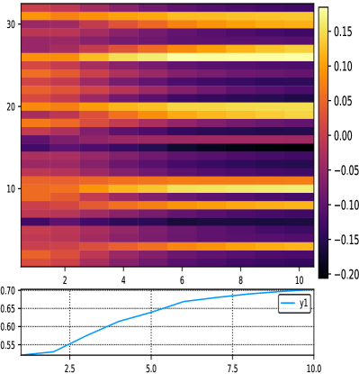
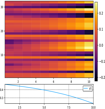
(a) Worsening progression ($P=0.70$)	(b) Improving progression ($P=0.23$)

Figure 2: Illness state progression over time, measured as $\boldsymbol{h}_{t}$ for the last 10 visits. Left figure: a high-risk case with 70% chance of readmission at time T=10. Right figure: a low-risk case with 23% chance at the end of the sequence. Best viewed in color.

Code embedding also reveals the space of diseases, as visualized in Fig. 3.

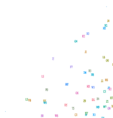
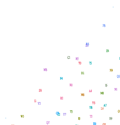
(a) Diabetes related diseases	(b) Mental health related

Figure 3: Projection of ICD-10 diagnostic codes using t-SNE after embedding. Best viewed in color. Interested readers are referred to the WHO official ICD-10 scheme book [http://apps.who.int/classifications/icd10/browse/2010/en].

V Discussion

We have taken an algebraic view of healthcare in that medical artifacts are represented as algebraic objects such as vectors and tensors. The continuous representation of diseases make it easy to study the disease space, that is, which diseases are related and may be interacting. The same holds for the treatments, and the clinic visits. The view also allows natural modelling of the evolution of illness as a result of the interaction between multiple diseases and multiple treatments over time. More specifically, we have argued for representing a healthcare trajectory as a sequence of (interaction of) sets, which is then realized by our new model dubbed $\mathsf{\mathtt{Resset}}$. The model employs a simple multi-valued set function for diseases and for treaments. Multi-disease–multi-treatment interaction per visit is a dual-input function of the two set functions. A healthcare trajectory is then modelled using LSTM for its capability of memorizing distant events. Importantly, the entire system is end-to-end: the model reads the medical record and predicts future risks without any manual feature engineering. Results on over a hundred thousand visits by patients suffering from chronic conditions, diabetes and metal health, demonstrate the usefulness of the model.

Future work will refine $\mathsf{\mathtt{Resset}}$ in the healthcare context to address the irregular timing of visits, more comprehensive set functions (e.g., with self-attention), interaction functions, and predicting sequence of sets. We wish to emphasize here that $\mathsf{\mathtt{Resset}}$ can be tailored to other problems of sequence of sets. For example, a video is a sequence of shots, each of which is a set of objects and actions.

References

- [1] Léon Bottou. From machine learning to machine reasoning. Machine Learning, 94(2):133–149, 2014.
- [2] Yu Cheng, Fei Wang, Ping Zhang, and Jianying Hu. Risk prediction with electronic health records: A deep learning approach. In SIAM International Conference on Data Mining (SDM 2016). SIAM, 2016.
- [3] Edward Choi, Mohammad Taha Bahadori, Elizabeth Searles, Catherine Coffey, and Jimeng Sun. Multi-layer representation learning for medical concepts. KDD, 2016.
- [4] Edward Choi, Mohammad Taha Bahadori, Jimeng Sun, Joshua Kulas, Andy Schuetz, and Walter Stewart. RETAIN: An Interpretable Predictive Model for Healthcare using Reverse Time Attention Mechanism. In Advances in Neural Information Processing Systems, pages 3504–3512, 2016.
- [5] Ronan Collobert, Jason Weston, Léon Bottou, Michael Karlen, Koray Kavukcuoglu, and Pavel Kuksa. Natural language processing (almost) from scratch. The Journal of Machine Learning Research, 12:2493–2537, 2011.
- [6] Jeffrey L Elman. Finding structure in time. Cognitive science, 14(2):179–211, 1990.
- [7] Andre Esteva, Brett Kuprel, Roberto A Novoa, Justin Ko, Susan M Swetter, Helen M Blau, and Sebastian Thrun. Dermatologist-level classification of skin cancer with deep neural networks. Nature, 542(7639):115–118, 2017.
- [8] Hayit Greenspan, Bram van Ginneken, and Ronald M Summers. Guest editorial deep learning in medical imaging: Overview and future promise of an exciting new technique. IEEE Transactions on Medical Imaging, 35(5):1153–1159, 2016.
- [9] Varun Gulshan, Lily Peng, Marc Coram, Martin C Stumpe, Derek Wu, Arunachalam Narayanaswamy, Subhashini Venugopalan, Kasumi Widner, Tom Madams, Jorge Cuadros, et al. Development and validation of a deep learning algorithm for detection of diabetic retinopathy in retinal fundus photographs. Jama, 316(22):2402–2410, 2016.
- [10] S Hamid Rezatofighi, BG Kumar, Anton Milan, Ehsan Abbasnejad, Anthony Dick, Ian Reid, et al. Deepsetnet: Predicting sets with deep neural networks. In Proceedings of the IEEE Conference on Computer Vision and Pattern Recognition, pages 5247–5256, 2017.
- [11] Sepp Hochreiter and Jürgen Schmidhuber. Long short-term memory. Neural computation, 9(8):1735–1780, 1997.
- [12] David M Kent and Rodney A Hayward. Limitations of applying summary results of clinical trials to individual patients: the need for risk stratification. Jama, 298(10):1209–1212, 2007.
- [13] Diederik Kingma and Jimmy Ba. Adam: A method for stochastic optimization. arXiv preprint arXiv:1412.6980, 2014.
- [14] David Krueger and Roland Memisevic. Regularizing RNNs by Stabilizing Activations. arXiv preprint arXiv:1511.08400, 2015.
- [15] Yann LeCun, Yoshua Bengio, and Geoffrey Hinton. Deep learning. Nature, 521(7553):436–444, 2015.
- [16] Phuoc Nguyen, Truyen Tran, Nilmini Wickramasinghe, and Svetha Venkatesh. Deepr: A Convolutional Net for Medical Records. Journal of Biomedical and Health Informatics, 21(1), 2017.
- [17] Trang Pham, Truyen Tran, Dinh Phung, and Svetha Venkatesh. Predicting healthcare trajectories from medical records: A deep learning approach. Journal of biomedical informatics, 69:218–229, 2017.
- [18] Trang Pham, Truyen Tran, and Svetha Venkatesh. One size fits many: Column bundle for multi-x learning. arXiv preprint arXiv:1702.07021, 2017.
- [19] Daniele Ravì, Charence Wong, Fani Deligianni, Melissa Berthelot, Javier Andreu-Perez, Benny Lo, and Guang-Zhong Yang. Deep learning for health informatics. IEEE Journal of Biomedical and Health Informatics, 21(1):4–21, 2017.
- [20] Benjamin Shickel, Patrick James Tighe, Azra Bihorac, and Parisa Rashidi. Deep EHR: A Survey of Recent Advances in Deep Learning Techniques for Electronic Health Record (EHR) Analysis. IEEE Journal of Biomedical and Health Informatics, 2017.
- [21] Truyen Tran. Deep learning for biomedicine: A tutorial. ACML, Seoul, Korea. URL: https://truyentran.github.io/acml17-tute.html, 2017.
- [22] Truyen Tran, Tu Dinh Nguyen, Dinh Phung, and Svetha Venkatesh. Learning vector representation of medical objects via EMR-driven nonnegative restricted Boltzmann machines (eNRBM). Journal of biomedical informatics, 54:96–105, 2015.
- [23] Ashish Vaswani, Noam Shazeer, Niki Parmar, Jakob Uszkoreit, Llion Jones, Aidan N Gomez, Lukasz Kaiser, and Illia Polosukhin. Attention is all you need. NIPS, 2017.
- [24] Oriol Vinyals, Samy Bengio, and Manjunath Kudlur. Order matters: Sequence to sequence for sets. ICLR, 2016.
- [25] Deniz Yuret. Knet: beginning deep learning with 100 lines of julia. In Machine Learning Systems Workshop at NIPS 2016, 2016.
- [26] Manzil Zaheer, Satwik Kottur, Siamak Ravanbakhsh, Barnabas Poczos, Ruslan Salakhutdinov, and Alexander Smola. Deep sets. NIPS, 2017.